Mott Transition and Volume Law Entanglement with Neural Quantum States

Abstract

The interplay between delocalisation and repulsive interactions can cause electronic systems to undergo a Mott transition between a metal and an insulator. Here we use neural network hidden fermion determinantal states (HFDS) to uncover this transition in the disordered, fully-connected Hubbard model. Whilst dynamical mean-field theory (DMFT) provides exact solutions to physical observables of the model in the thermodynamic limit, our method allows us to directly access the wavefunction for finite system sizes well beyond the reach of exact diagonalisation. We directly benchmark our results against state-of-the-art calculations obtained using a Matrix Product State (MPS) ansatz. We demonstrate how HFDS is able to obtain more accurate results in the metallic regime and in the vicinity of the transition, with the volume law of entanglement exhibited by the system being prohibitive to the MPS ansatz. We use the HFDS method to calculate the amplitudes of the wavefunction, the energy and double occupancy, the quasi-particle weight and the energy gap, hence providing novel insights into this model and the nature of the transition. Our work paves the way for the study of strongly correlated electron systems with neural quantum states.

Neural quantum states (NQS) are transforming the field of variational wave-functions for the quantum many-body problem. Originally introduced for models of interacting quantum spins Carleo and Troyer (2017), these methods have been generalized to interacting fermions for lattice models Inui et al. (2021); Stokes et al. (2020a); Nomura et al. (2017); Nys and Carleo (2022); Luo and Clark (2019); Moreno et al. (2022), small molecular systems Xia and Kais (2018); Choo et al. (2020); Yang et al. (2020); Sureshbabu et al. (2021); Yoshioka et al. (2021); Rath and Booth (2023); Barrett et al. (2022); Zhao et al. (2023) and systems in continuous space Ruggeri et al. (2018); Pfau et al. (2020); Spencer et al. (2020); Hermann et al. (2020); Entwistle et al. (2023); von Glehn et al. (2022); Cassella et al. (2023); Pescia et al. (2023); Kim et al. (2023); Lou et al. (2023); Lovato et al. (2022); Fore et al. (2022). Electron interactions can turn a metal into an insulator: this is the Mott phenomenon, which plays a central role in the physics of materials with strong electronic correlations. It is therefore relevant to ask whether NQS are able to describe both a correlated metallic phase and a Mott insulating phase, as well as the transition between them. The question is especially pertinent when the Mott insulating phase does not have long-range magnetic order in the ground-state, a notorious challenge to the expressivity of variational wave-functions Becca and Sorella (2017).

Here, we address this by considering one of the simplest models in which such a transition occurs: the fully connected fermionic Hubbard model with random hopping amplitudes. This model is challenging for variational methods since, as shown below, it displays an entanglement entropy which scales with the number of sites. While hugely successful in low-dimensional and tree-like systems Orús (2019); Tindall et al. (2020, 2023), we find here that representing the wave-function as a matrix product state (MPS) and optimizing it with the density-matrix renormalization group (DMRG) algorithm White (1992, 1993, 2005); Schollwöck (2011); Rommer and Östlund (1997); Jeckelmann (2002) requires prohibitively large bond dimensions. Consequently, convergence can be achieved only up to moderate system sizes.

On the other hand, dynamical mean-field theory (DMFT) Georges et al. (1996), which exploits locality rather than low entanglement, provides an exact framework in which the properties of this model in the limit of an infinite number of sites can be computed rather seamlessly with modern algorithms. This provides a controlled benchmark to which variational methods can be compared. Being a Green’s function based method, however, DMFT does not provide access to the many-body wave-functions of the system, so that basically nothing is known about them aside from the qualitative properties summarized below .

In this article, we study this model with the recently introduced neural network hidden fermion determinantal states (HFDS) Moreno et al. (2022). We show that this method performs successfully both in the metallic and Mott insulating phases. It is also able to clearly reveal the Mott transition, although accuracy is challenging in this regime. We show that while large-scale DMRG calculations working in the position basis also reveal the transition, for small interaction strengths and near the transition they incur a higher computational cost. We also demonstrate that the performance of DMRG can be significantly improved by optimizing the basis of single-particle states. Our work provides a new wave-function based perspective on this model, and paves the way to the study of physical phenomena associated with strong fermionic correlations correlations with NQS.

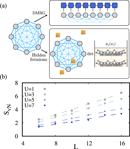
Figure 1: Panel (a): Schematic of the fully connected random hopping Hubbard model and the DMRG and HFDS methods. Panel (b): Von-Neumann entanglement entropy of a random bipartition for the ground state of this model for various $U$ as a function of system size $L$, computed using DMRG with a maximum bond dimension of $32,000$. Dashed lines correspond to a linear fitting of the data.

Model.

- We consider the fully connected fermionic Hubbard model of $L$ sites with random hopping amplitudes (Fig. 1) defined by the Hamiltonian:

$$H=-\frac{1}{\sqrt{L}}\sum_{\begin{subarray}{c}i,j=1\\ i\neq j\\ \end{subarray}}^{L}\sum_{\sigma\in\{\uparrow,\downarrow\}}\,t_{ij}\,c^{\dagger}_{i,\sigma}c_{j,\sigma}+U\sum_{i=1}^{L}\hat{n}_{i,\uparrow}\hat{n}_{i,\downarrow},$$ (1)

where $c^{\dagger}_{i,\sigma}$ and $c_{i,\sigma}$ are, respectively, the creation and annihilation operators for a fermion of spin $\sigma$ on site $i$. We have defined the number operator $\hat{n}_{i,\sigma}=c^{\dagger}_{i,\sigma}c_{i,\sigma}$. The $L(L-1)/2$ hopping amplitudes $t_{ij}$ are random variables drawn independently from the Gaussian normal distribution with mean $0$ and standard deviation $1$, i.e. $\overline{t_{ij}}=0$ and $\overline{t^{2}_{ij}}=t^{2}=1$. We fix $t=1$ as our unit of energy. Throughout this work, we consider the half-filled case with, on average, one electron per site ($N=L$).

In the infinite-volume, this model is known to possess self-averaging properties Chowdhury et al. (2022). Local observables such as the double occupancy $d_{i}=\langle\hat{n}_{i\uparrow}\hat{n}_{i\downarrow}\rangle$ have sample-to-sample fluctuations which vanish as $L\rightarrow\infty$ and thus converge with probability one to their sample-averaged values denoted by $\overline{\cdots}$: $d_{i}\rightarrow\overline{\langle\hat{n}_{i\uparrow}\hat{n}_{i\downarrow}\rangle}$. For the wavefunction methods at finite $L$, we perform sample averages over $20$ realizations of the disorder for each value of $U$ and each system size. Unless stated otherwise, physical quantities shown in the plots are averaged over these realizations and the standard deviation is used as an estimation of the error bars. We use identical realizations for both DMRG and HFDS.

We now briefly summarize the known zero-temperature properties of the model obtained from DMFT for $L\rightarrow\infty$. For $U=0$, the spectrum of one-particle eigenstates is obtained by diagonalizing the random matrix $t_{ij}$ and the density of states obeys a Wigner semi-circular law of bandwidth $4t$. As $U$ is turned on, the ground-state is a Fermi liquid metal up to a critical value $U=U_{c2}$. The most accurate NRG solutions of the DMFT equations report $U_{c2}=5.82...$ Lee et al. (2017). Note that this model does not host a superconducting ground-state in the repulsive case $U>0$: Kohn-Luttinger instabilities to non-local order parameters cannot occur, a peculiarity of the infinite connectivity. The Fermi liquid state is therefore stable down to $T=0$ for $U<U_{c2}$. For $U>U_{c2}$, the ground-state is a Mott insulator. For any finite $U$, however, charge fluctuations survive and the double occupancy remains non-zero.

The physics of the system in the Mott phase is best understood qualitatively by thinking of the large-$U$ limit. There, and as $L\rightarrow\infty\,$, the Hamiltonian reduces at half-filling to $\sim\frac{4t^{2}}{UL}\left(\sum_{i}\vec{S}_{i}\right)^{2}$ which is exactly solvable Georges and Krauth (1993); Rozenberg et al. (1994); Laloux et al. (1994). It has an exponentially degenerate manifold of singlet ground-states, so that the $T=0$ thermodynamic entropy is non-zero and extensive $\sim L\ln 2$. We expect, however, the ground-state to be non-degenerate for a finite size $L$ and a given sample $t_{ij}$. Note that due to the all-to-all hopping, the system is fully frustrated and cannot host a ground-state with Néel order.

This model thus arguably provides one of the simplest examples of a system having a $T=0$ phase transition between a metallic Fermi liquid ground-state and a Mott insulating state with no magnetic long-range order. The phase transition occurs at $U_{c2}$ and is known to be second-order Rozenberg et al. (1994); Georges et al. (1996), with the energy and double occupancy being continuous through the transition. A subtle point is that the insulating solution exists as a metastable, higher energy, solution in a window of coupling $U\in[U_{c1},U_{c2}]$, with $U_{c1}=4.74\cdots$ Lee et al. (2017). This holds for the infinite-volume limit, but the consequences for finite-$L$ are not currently known.

From a wavefunction point of view, this model is challenging since it has volume-law entanglement. In Fig. 1b, we evidence this: computing the half-system bi-partite von-Neumann entanglement entropy $S$ of the ground state as a function of $L$, up to $L=16$, for a range of $U$. For all values of $U$ a clear linear dependence of $S$ with system size is observed – suggesting that for any finite $U$ in the position basis the entanglement entropy follows a volume law. Recently, it has been argued that in practice deep and shallow feed-forward NQS are not capable of efficiently representing ground states with volume-law entanglement Passetti et al. (2023). Referecne  Passetti et al. (2023), however, never considered functional parametrizations containing determinants, like Slater-Jastrow Nomura et al. (2017); Stokes et al. (2020a), backflow Luo and Clark (2019) or HFDS Moreno et al. (2022) parametrizations. In the study of fermionic systems, determinant-based functional parametrizations play a fundamental role in the representability of the ground state, regardless of the amount of entanglement. For example, the entanglement of the ground state of Hamiltonian in Eq.( 1) at $U=0$ follows a volume law in the localized basis. Despite this, it can be exactly represented by a Slater determinant.

Methods.

The HFDS formalism is based on an augmentation of the physical Fock space (which is spanned by $M=2L$ ‘visible’ fermionic degrees of freedom) by $\tilde{M}$ additional ‘hidden’ modes, resulting in $M_{\textrm{tot}}=M+\tilde{M}$ degrees of freedom. The physical Fock space is recovered by a projection procedure, which assigns a unique state $\tilde{n}=F(n)$ of the hidden fermions to each Fock state $n=\{n_{i\sigma}\}$ ($n_{i\sigma}=0,1$) of the physical/visible fermions. The wave-function amplitude corresponding to the occupancy $n$ in the physical subspace, is given by:

$$\psi(n)=\langle n,F(n)|\Psi\rangle,$$ (2)

where $|\Psi\rangle$ is a many-body state in the augmented space. A powerful variational state is obtained when both $|\Psi\rangle$ and $F(n)$ belong to a parametric family. In this work, following the construction in Ref. Moreno et al. (2022), $|\Psi\rangle$ is taken to be a Slater determinant with $N$ visible and $\tilde{N}$ hidden fermions, and $F(n)$ is an internal state in a neural network. When projected onto the physical space, this yields a correlated wavefunction. For lattice models, it can be shown that this ansatz is universal and is explicitly connected to configuration-interaction states Moreno et al. (2022); Robledo Moreno (2023). The amplitudes $\psi(n)$ are optimized using Variational Monte Carlo (VMC).

The second method we use is DMRG White (1992); Schollwöck (2011). We initialise our approximation for the ground state wavefunction as a product-state MPS and repeatedly perform DMRG sweeps, enforcing a bond dimension $\chi\leq\chi_{\rm max}$. We utilize both $U(1)$ symmetries of the model – restricting ourselves to half-filling and $\langle S^{z}\rangle=0$. For system sizes $L\leq 16$ we use a sufficient bond-dimension ($\chi_{\rm max}=32,000$) to observe convergence of the energy. For $U=0$ and $L=16$, this means we reach an energy within $0.001\%$ of the true ground-state energy. This is an extremely large bond dimension given the size of this system and is indicative of the difficulty of the problem at hand for the DMRG algorithm. For $L>16$ and any $U$ we are unable to achieve convergence in energy and use the largest bond-dimension ($\chi_{\rm max}\sim 10^{4}$) that we can afford with our available computational resources. Further details are provided in the Supplemental Material (SM)  sup . There, we also show how DMRG calculations can be made more efficient by optimizing the basis of single-particle states, following the technique described in Ref. Moreno et al. (2023).

Results.

In Figures 2 and 3 we report results obtained by computing the ground-state wave-function using the HFDS and DMRG methods. We display: the structure of the wave function in the space of electronic configurations, the energy and double occupancy per site and the energy gap.

In order to understand the structure of the wave function in the space of electronic configurations, we study the weight of the wave function amplitudes for electronic configurations $n_{d}$ with double occupancy $d$: $\mathcal{W}(d)=\sum_{n_{d}}|\psi(n_{d})|^{2}$. This quantity can be estimated as the ratio of sampled configurations with double occupancy $d$ when sampling $n_{d}\sim|\psi|^{2}$. Panel (a) in Fig. 2 shows a bar plot of these weights, obtained with the HFDS ansatz for a system with $L=32$, which is beyond the reach of exact diagonalization. For small values of $U$ in the metallic phase, the wave function spreads across electronic configurations with a wide range of double occupancy. Close to the transition point, the weight shifts towards configurations with $d=0$ and $d=1$. For large values of $U$ in the Mott insulating phase, the weight of the wave function in each sub-sector of double occupancy decays exponentially with $d$ and peaks around $d=0$. Panel (b) in Fig. 2 shows the weight of the wavefunction for $d=0$, $d=1$ and $d>0$ as a function of $U$. We observe that the point where the weight of the wavefunction becomes dominated by electronic configurations with $d=0$ coincides with the metal-insulator transition, thus providing a signature of the phase transition. For more details see  sup .

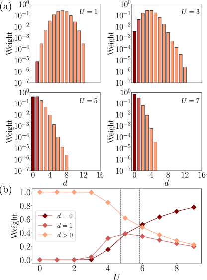
Figure 2: (a) Weight of the HFDS wave function for electronic configurations with double occupancy $d$ (as defined in the main text), for $L=32$ and different values of $U$. Darker to lighter colors indicate $d=0$, $d=1$ and $d>1$ respectively, as related to panel (b). (b) Wavefunction weight versus $U$ for different values of the double occupancy as indicated. The dashed vertical lines indicate the values of $U_{c1}$ and $U_{c2}$ for $L=\infty$ as obtained from DMFT.

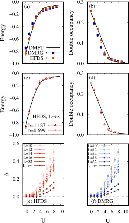
Figure 3: Top panel: Ground state energy per site (a) and double occupancy (b) as a function of the Hubbard interaction strength $U$. Results are shown from HFDS (orange circles), DMRG (blue squares) for $L=32$ and DMFT+NRG (black line) calculations for $L=\infty$. Middle panel: Ground state energy (c) and double occupancy (d) obtained from a finite-size extrapolation to $L\rightarrow\infty$ of the HFDS results. The extrapolation is done using the formula $f(L)=A/L^{b}+f(L\rightarrow\infty)$. Details on the finite-size extrapolations and on the choice of $b$ are available in the SM sup . Bottom Panel: Energy gap as a function of $U$ obtained from HFDS (e) and DMRG (f) for various $L$. Details of the $L\rightarrow\infty\,$extrapolation are available in sup .

We compare the predictions from the wavefunction methods to DMFT+NRG data for $L=\infty$ in Fig. 3 (a-d). The DMFT+NRG is obtained in a state-of-the-art NRG implementation Peters et al. (2006); Weichselbaum and von Delft (2007); Žitko and Pruschke (2009); Lee and Weichselbaum (2016) based on the QSpace tensor library Kugler (2022). In panels (a) and (b) of Figure 3, we plot the ground-state energy per site and the double occupancy, respectively, as a function of $U$ for $L=32$.

The results obtained from both methods are overall in good qualitative agreement with the DMFT ground-state results, even though the latter apply to the $L\rightarrow\infty\,$limit. At this system size and values of $U\leq 4$, the accuracy of the HFDS surpasses that of the DMRG, achieving lower variational energies and better agreement with the DMFT double occupancies. This noticeable difference persists for increasing system sizes, and in the SM sup we compare results for $L=48$ and show how the DMRG calculation obtains a far higher ground-state energy despite requiring extensive computational resources. We also note that the DMRG results for the double occupancy are in better agreement with the HFDS and DMFT in the insulating phase. This may be expected since this phase has lower entanglement (Fig. 1(b)) making it more favorable for DMRG in the position basis. Finite-size effects are also expected to be smaller in that phase. In panels (c) and (d) of Figure 3, we display the same observables extrapolated to $L\rightarrow\infty\,$within the HFDS method (see sup for details). The extrapolated values are in good quantitative agreement with the DMFT data, except for values of $U$ in the range $U\simeq 4$ to $U\simeq 6$, corresponding to the vicinity of the Mott transition. As mentioned above, a metastable insulating solution is known to exist for $L\rightarrow\infty\,$in this range of coupling. It is unclear whether the observed discrepancy between both the HFDS and DMRG results and the DMFT data in this range of $U$ is due to finite-size effects, or if this difference is rather due to the wavefunction-based approaches finding the metastable insulating state, which might also be more stable at finite $L$.

We also study observables beyond the ground-state to quantify the metal-to-insulator transition from our wavefunction methods, focusing on the ground-state energy gap $\Delta$:

$$\Delta=E(N+1)+E(N-1)-2E(N),$$ (3)

where $E$ is the ground state energy averaged over $20$ realizations of the disorder, and $N=L$ is the number of particles at half filling. The results obtained with HFDS and DMRG are reported in panels (e) and (f) of Figure 3, respectively, for various sizes $L$. An extrapolation to $L\rightarrow\infty\,$is also displayed.

The gap extrapolated to $L\rightarrow\infty\,$has a behavior qualitatively similar to the $L=32$ results: it is close to $0$ at low values of $U$, and increases above $U=4$, the extrapolated value being clearly non-zero for $U=5$ in both DMRG and HFDS. Indeed, the gap of the metastable insulator opens at $U_{c1}=4.74\cdots$ in the $L=\infty$ DMFT solution. In this limit, however, the ground-state remains a metal up to $U_{c2}=5.82\cdots$. This again can be interpreted either as the HFDS and DMRG methods picking up a metastable insulating solution in the Mott transition region or as much larger system sizes being necessary to stabilize the true metallic ground-state for $U\in[U_{c1},U_{c2}]$.

As an alternative way of characterizing the Mott transition, we also computed the quasiparticle weight $Z$ from the density matrix, finding good agreement with the DMFT-computed values of $Z$, as reported in the SM sup .

Conclusion.

The results shown above and in the SM sup demonstrate that the HFDS and DMRG approaches can be used to solve the fully-connected random hopping Hubbard model for finite system sizes. We showed results for $L=32$ sites, which is far beyond what can be achieved with exact diagonalization. We also present, in sup , computations with $L=48$. We find that, for $L=32$ in the metallic regime, the HFDS approach performs better than the DMRG and yields a lower variational ground-state energy. The DMRG results we obtain for smaller system sizes ($L\leq 16$) are essentially exact, but the method becomes limited computationally for larger systems. The HFDS calculations require comparatively less computational resources than DMRG for the same system size. In the intermediate coupling regime where metallic and insulating solutions are known from DMFT to coexist in the infinite-volume limit, the question of the accuracy of the ground state that is found by our variational calculations is still unclear. Calculations for larger system sizes may elucidate this issue. We found nonetheless that our calculations are able to clearly identify the Mott transition in this model.

While DMFT provides an exact, Green’s function based, numerical solution of this model in the infinite volume limit, the nature of its ground-state wavefunction and how it changes through the Mott transition were uncharted territory up to now. Our work resolves this by providing a direct determination of this wavefunction. Extensions to closely related models, e.g. of the SYK type Chowdhury et al. (2022), could be considered in future studies. Our work furthermore demonstrates that neural quantum states can be used efficiently for the study of fermionic problems with volume-law entanglement, in contrast to a recent claim Passetti et al. (2023) (see also Denis et al. (2023)). By demonstrating that the iconic Mott transition can be captured by such approaches, our work paves the road for the study of the physics of strong electronic correlations with neural quantum states.

.1 Supplementary Material to ‘Mott Transition and Volume Law Entanglement with Neural Quantum States’

.2 Details of DMRG Calculations

In the DMRG calculations we utilise the ITensor Library to build the long-range Hamiltonian in Eq. 1 as a MPO and encode our ansatz for the ground state as a MPS. The ordering of the sites is chosen randomly due to the the long-range disordered nature of the Hamiltonian.

In Fig. S1a we plot the average truncation error from the SVD’s performed in the final (20th) sweep of the calculation for a range of bond-dimensions and for $L=16$ The results are averaged over the same $20$ instances of disorder as in the main text. A systematic improvement is seen with increasing bond-dimension and for $\chi=32,000$ the largest error is on the order of $10^{-6}$ for small $U$. We also plot, for $U=0$, the percentage difference (again averaged over disorders) between the energy density of the state found via DMRG and the exact energy found via diagonalisation of the hopping matrix. For $\chi=32,000$ the percentage error drops below $0.001\%$. Given that for $U=0$ our truncation errors are largest, we are confident this means the energies we have found via DMRG for $L=16$ throughout the phase diagram are accurate to within $0.001\%$ or better.

We also plot, in Figs. S1c and d, the results for $L=32$. Here, for the largest bond-dimension obtainable ($\chi\sim 8,000$), we reach truncation errors on the order of $10^{-3}$ for small $U$, indicating a significantly more inaccurate calculation than for $L=16$. This is evidenced by our plots of the convergence of energy versus $U$ and $\chi$, where the ground state energy we find has clearly not converged yet with increasing bond-dimension. We also include an inset for $U=1.0$, $\chi=8000$ and a specific instance of disorder. Here we show the change in energy vs DMRG sweep and as we increase the bond-dimension to its maximum value we see this converge with sweep number — indicating that our DMRG calculations have converged for the given bond dimension.

Finally, in in Figs. S1e, we plot results for $L=48$, $U=3.0$ and a single disorder instance. We show the DMRG found energy (after $20$ sweeps) versus bond dimension and also indicate the result found via HFDS for the same disorder instance, system size and interaction strength. The HFDS result is far below the DMRG result despite the DMRG result requiring over $4$ days of Walltime and $5$GB of RAM on a $64$ core icelake node of our Rusty supercomputing cluster with multithreading enabled.

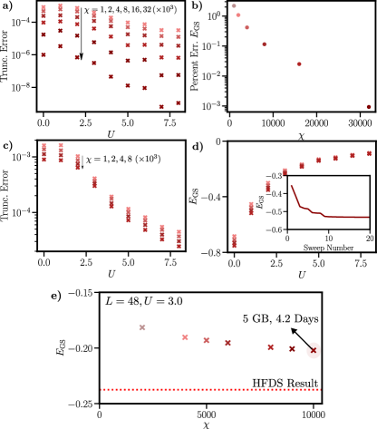
Figure S1: Numerical Details of DMRG calculations for bond-dimensions increasing up to the values used in the main text. a) Average sum of square of singular values thrown away during SVD’s in the final sweep of the DMRG calculation. Data is for $L=16$ averaged over $20$ disorders for a range of $U$ and $\chi$ values. b) Percentage error on the energy found in the DMRG calculation versus $\chi$ and for $L=16$, $U=0.0$. c) Average sum of square of singular values thrown away during SVD’s in the final sweep of the DMRG calculation. Data is for $L=32$ averaged over $20$ disorders for a range of $U$ and $\chi$ values. d) Energy of the result of the DMRG calculation for $L=32$ and a range of $\chi$ and $U$ values. Inset) Convergence of energy with DMRG sweep number for a single disorder instance, $L=32,U=1.0$ and $\chi=8\times 10^{3}$. e) Energy of the result of the DMRG calculation for $L=48$, a range of $\chi$ values, $U=3.0$ and a single disorder instance. The point at $\chi=10000$ is annotated with the RAM and walltime required by the simulation. The red dotted line shows the energy obtained from the corresponding HFDS calculation for exactly the same Hamiltonian.

.3 Optimizing the single-particle basis set for DMRG calculations

For the sake of completeness, we emphasize that the scaling of the entanglement entropy, which is the limiting factor in DMRG, is strongly dependent on the single-particle basis used to represent the Hamiltonian. In order to mitigate this effect, we follow the procedure discussed in Ref. Moreno et al. (2023) to make the DMRG technique invariant under the reparametrization of $H$ corresponding to rotations of the single-particle basis. Every three sweeps, the one- and two-body reduced-density-matrices are measured and gradient descent techniques are used to find the single-particle basis that minimizes the energy. A total of thirty sweeps are performed in total. Fig. S2 demonstrates the improvement in the ground state energy resulting from this procedure. The difference (see inset) between the ground-state energy obtained from DMRG in the fixed localized basis and when including basis optimizations is larger in the metallic phase and vanishes in the insulating phase, where the ground state is localized and therefore the localized basis is the optimal basis choice for the DMRG. This observation can be exploited to obtain additional diagnostics for the Mott transition. This will be the focus of future investigations.

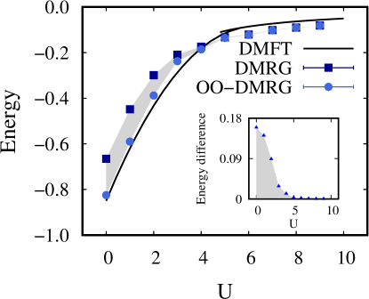
Figure S2: Ground state energy per site as a function of $U$ obtained with DMRG in the fixed localized basis (DMRG) and in an optimized single-particle basis (see text). The system size is $L=24$ and $\chi_{\textrm{max}}=800$ in both cases and the results are averaged over the same $20$ disorder realisations in each case. The shaded region highlights the energy improvement and the inset displays shows the difference in energy between the two approaches as a function of $U$.

.4 Details of the VMC calculation with Hidden-Fermion Determinant States

As described in the main text, VMC is performed within the hidden-fermion formalism, where the basis for the augmented Fock space is spanned by the set of states:

$$|n,\tilde{n}\rangle=\left(\prod_{i,\sigma}\left(\hat{a}^{\dagger}_{i\sigma}\right)^{n_{i\sigma}}\right)\left(\prod_{1\leq\mu\leq\tilde{M}}\left(\hat{d}^{\dagger}_{\mu}\right)^{\tilde{n}_{\mu}}\right)|0\rangle,$$ (S1)

where $\hat{a}^{\dagger}_{i\sigma}$ and $\hat{d}^{\dagger}_{\mu}$ are the creation operators for the visible and hidden modes respectively. The previous definition assumes the canonical ordering where the operators closest to the Fock vacuum are those with the largest mode index. VMC in the physical subspace requires the definition of the wave function amplitudes of the trial state $|\Psi\rangle$ projected into the physical subspace, as described by Eq. 2 in the main text.

$|\Psi\rangle$ is chosen as the Slater determinant in the augmented Fock space characterized by a number $N_{\textrm{tot}}=N+\tilde{N}$ of orbital functions $\phi_{n}:\{1,\ldots,M_{\textrm{tot}}\}\mapsto\mathbb{R}$ with $1\leq n\leq N_{\textrm{tot}}$:

$$|\Psi\rangle=\hat{\varphi}^{\dagger}_{1}\ldots\hat{\varphi}^{\dagger}_{N_{\textrm{tot}}}|0\rangle.$$ (S2)

The new set of creation operators $\hat{\varphi}^{\dagger}_{\alpha}$ is a linear combination of the visible and hidden creation operators defined by:

$$\left(\hat{\varphi}^{\dagger}_{1},\ldots,\hat{\varphi}^{\dagger}_{N_{\textrm{tot}}}\right)=\left(\hat{a}^{\dagger}_{1},\ldots,\hat{a}^{\dagger}_{M},\hat{d}^{\dagger}_{1},\ldots,\hat{d}^{\dagger}_{\tilde{M}}\right)\cdot\Phi.$$ (S3)

$\Phi\in\mathbb{R}^{M_{\textrm{tot}}\times N_{\textrm{tot}}}$ is the matrix of optimizable orbitals, whose columns define the orbital functions. Following Ref. Moreno et al. (2022), the matrix of orbitals is decomposed into blocks:

$$\Phi=\begin{bmatrix}\phi_{\rm v}&\chi_{\rm v}\\ \phi_{\rm h}&\chi_{\rm h}\end{bmatrix}\enspace.$$ (S4)

Where $\phi_{\rm v}\in\mathbb{R}^{M\times N}$ is the matrix representing the amplitudes of the visible orbitals evaluated in the visible modes, $\chi_{\rm v}\in\mathbb{R}^{M\times\tilde{N}}$ is the matrix representing the amplitude of the hidden orbitals evaluated in the visible modes, $\phi_{\rm h}\in\mathbb{R}^{\tilde{M}\times N}$ is the matrix representing the amplitude of the visible orbitals evaluated in the hidden modes and $\chi_{\rm h}\in\mathbb{R}^{\tilde{M}\times\tilde{N}}$ is the matrix representing the amplitude of the hidden orbitals evaluated in the hidden modes.

In the VMC framework particle configurations ($x=(x_{1},\ldots,x_{N})$ and $\tilde{x}=(\tilde{x}_{1},\ldots,\tilde{x}_{\tilde{N}})$ for visible and hidden fermions respectively) are sampled instead of occupations. $|x,\tilde{x}\rangle$ states differ from $|n,\tilde{n}\rangle$ states in that the application of the creation operators to the Fock vacuum does not follow the canonical order of Eq. S1 and instead follows the order specified by the particle index labels in $x$ and $\tilde{x}$. The constraint used to project the trial state to the physical subspace $F(n)$ can be translated into a constraint function in the space of particle configurations:

$$f:x\mapsto\tilde{x},$$ (S5)

where $f$ is chosen to be symmetric with respect to the particle indices of $x$. This constraint ensures that the Fermi statistics is preserved. The hidden-fermion determinant state wave function amplitudes in the space of particle configurations are then given by:

$$\psi(x)=\langle x,f(x)|\Psi\rangle=\det\begin{bmatrix}\phi_{\rm v}(x)&\chi_{\rm v}(x)\\ \phi_{\rm h}(f(x))&\chi_{\rm h}(f(x))\end{bmatrix}.$$ (S6)

$\big{[}\phi_{\rm v}(x)$, $\chi_{\rm v}(x)\big{]}$ and $\big{[}\phi_{\rm h}(f(x)),\chi_{\rm h}(f(x))\big{]}$ denote the $N\times(N+\tilde{N})$ and $\tilde{N}\times(N+\tilde{N})$ sub-matrices obtained from $\big{[}\phi_{\rm v},\chi_{\rm v}\big{]}$ and $\big{[}\phi_{\rm h},\chi_{\rm h}\big{]}$ respectively by slicing the row entries corresponding to $x$ and $f(x)$. The $\big{[}\phi_{\rm h}(f(x)),\chi_{\rm h}(f(x))\big{]}$ matrix is denoted as the hidden sub-matrix.

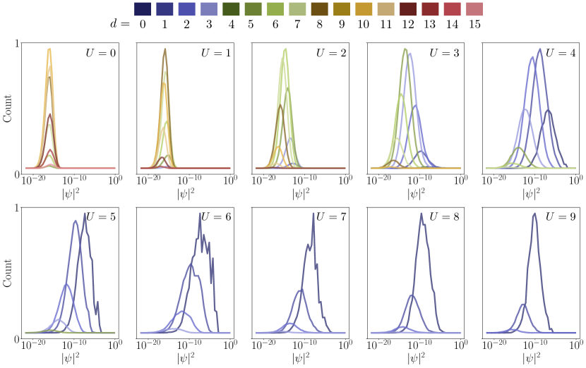
Figure S3: Histograms of the wave-function amplitudes obtained from HFDS for different values of $U$ as indicated in each panel. The wave function amplitudes are normalized using the norm estimate privided by Eq. S7. System size is $L=32$. Within each panel, the different colors show the histograms for the amplitudes evaluated at electronic configurations with double occupancy $d$, as indicated by each color.

Following the prescription of Ref. Moreno et al. (2022), the hidden sub-matrix can be materialized by the direct parametrization of the composition of the functions $\phi_{\textrm{h}}(f(x))$ and $\chi_{\textrm{h}}(f(x))$ by neural networks, whose input is the occupancy $n$ associated to the particle configuration $x$. This choice of parametrization automatically satisfies the permutation-symmetry requirements of $f(x)$. In practice, each of the $\tilde{N}$ rows of the hidden sub-matrix is parametrized by a two-layer perceptron with hyperbolic tangent activation functions. The number of hidden units in the hidden layer is characterized by the ratio $\alpha$ between the number of hidden units and the dimensionality of the input space ($2L$ in this case).

he complete set of variational parameters is given by the matrices $\phi_{\textrm{v}}$ and $\chi_{\textrm{v}}$ together with the weights and biases of the neural networks that parametrize the hidden sub-matrix. The hyper-parameters that control the expressive power of the ansatz are the number of hidden fermions $\tilde{N}$ and the width of the neural networks $\alpha$.

The wave function is optimized using the stochastic reconfiguration parameter update rule Sorella (1998); Sorella et al. (2007). The stochastic reconfiguration is the application of the natural gradient descent technique Amari (1998) to the optimization of quantum states Stokes et al. (2020b).

We observe that convergence to states with lower energies can be achieved if the optimization of the variational parameters is performed in two steps. First, the rows of the $\big{[}\phi_{\textrm{v}},\chi_{\textrm{v}}\big{]}$ matrix are fixed to be the $N+\tilde{N}$ Hartree-Fock orbitals of lowest energy (the Hartree-Fock orbitals are obtained using the PySCF Sun et al. (2020, 2018); Sun (2015) library), while the weights and biases of the hidden sub-matrix are optimized for a fixed number of iterations. This produces a compact representation of a wave function that contains the linear combination of all possible single, double, …, $\tilde{N}$-tuple excitations to the lowest $\tilde{N}$ virtual Hartree-Fock orbitals. Each factor of the linear combination carries a Jastrow factor determined by the hidden sub-matrix coefficients (see Ref. Moreno et al. (2022) for details). In the second step, both $\big{[}\phi_{\textrm{v}},\chi_{\textrm{v}}\big{]}$ are optimized with the weights and biases of the neural networks in the hidden sub-matrix.

.5 HFDS wave function amplitudes in the space of electronic configurations

In this appendix we study empirical statistics of the weight of the HFDS wave-function amplitudes for different subsets of electronic configurations and different values of $U$. The aim is to understand the structure of the ground-state wave function and its change as the value of $U$ is increased, changing character from a metal to an insulator, Since the model is disordered, the only distinguishing factor between subsets of electronic configurations is the number of doubly occupied sites $d$ on a given configuration $n$. Consequently, we focus on the analysis of the wave function amplitudes as a function of $d$ and $U$.

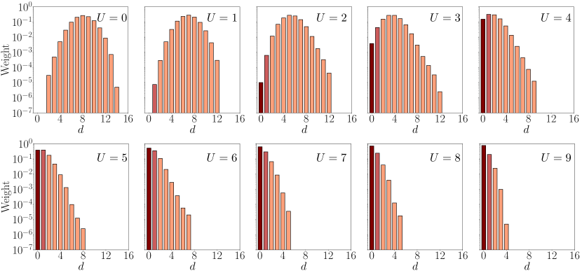
Figure S4: Weights of the HFDS wave function for electronic configurations $n_{d}$ with double occupancy $d$ as a function of $d$. System size is $L=32$ and different values of $U$ are shown in different panels. Darker to lighter colors indicate $d=0$, $d=1$ and $d>1$ respectively.

For the largest system size that we consider $(L=32)$, the direct enumeration of all possible electronic configurations is not feasible, since the dimensionality of the Hilbert space for this system size is $\mathcal{D}=\binom{32}{16}^{2}=3.6(1)\cdot 10^{17}$. Therefore, we restrict our statistical study to a subset of $20\cdot 10^{3}$ electronic configurations sampled for each $U$ and disorder realization according to the corresponding HFDS ground-state wave function amplitudes: $n\sim|\psi|^{2}$. Since the wave-function amplitudes are not required to be explicitly normalized for VMC calculations, the HFDS wave functions are not explicitly normalized. For the study of the wave function amplitudes as a function of $d$ and $U$, an unbiased estimate of the normalization factor can be obtained from the sampled electronic configurations:

$$\begin{split}\frac{1}{\sum_{n}|\psi(n)|^{2}}&=\frac{1}{\mathcal{D}}\sum_{n}\frac{1}{\sum_{n^{\prime}}|\psi(n^{\prime})|^{2}}=\frac{1}{\mathcal{D}}\sum_{n}\frac{|\bar{\psi}(n)|^{2}}{|\psi(n)|^{2}}\\ &\approx\frac{1}{\mathcal{D}}\mathbb{E}_{n\sim|\psi|^{2}}\left[\frac{1}{|\psi(n)|^{2}}\right],\end{split}$$ (S7)

where $\bar{\psi}(n)$ labels the explicitly normalized counterpart to $\psi(n)$: $\bar{\psi}(n)=\psi(n)/\sqrt{\sum_{n^{\prime}}|\psi(n^{\prime})|^{2}}$.

Figure S3 show the histogram of the normalized wave function amplitudes for different values of $U$, averaged over 20 disorder realizations. The histograms are grouped by the number of doubly occupied sited $d$ for the sampled electronic configurations. For $U<3$, the weight of the wave function is distributed across electronic configurations with a number of doubly occupied sites around $d\approx 8$. For small $U$, double occupancy does not significantly increase the energy of the system. Since the number of electronic configurations with double occupancy $d$ peaks at $d=8$, the wave function concentrates around $d=8$ for small $U$, dominated by a non-interacting character. For $U=3$ and $U=4$, as correlation increases but still in the metallic phase, the weight of the wave function starts shifting from electronic configurations with large numbers of the double occupancy to electronic configurations with $d\in[0,6]$. In particular, the fraction of sampled configurations with $d=0$ and $d=1$ starts to rapidly increase. At $U=5$, the weight of the wave function is concentrated in electronic configurations with $d\in[0,3]$. Interestingly, the height of the histogram for $d=0$ surpasses that of the histogram for $d=1$. For $U\geq 6$, the weight of the wave function concentrates around electronic configurations with $d=0$. However, the weight of electronic configurations with $d>0$ is only exactly suppressed in the $U\rightarrow\infty$ limit.

The information provided by the histograms in Fig. S3 can be further summarized by the weight of the wave function for electronic configurations $n_{d}$ with double occupancy $d$:

$$\mathcal{W}(d)=\sum_{n_{d}}\left|\psi(n_{d})\right|^{2},$$ (S8)

An unbiased estimator for $\mathcal{W}(d)$ can be obtained by the fraction of electronic configurations with double occupancy $d$ sampled according to $n_{d}\sim|\psi|^{2}$. Fig. S4 shows the weight of the wave function as a function of $d$ for different values of $U$, averaged over twenty disorder realizations. For small values of $U$ in the metallic phase, the wave function spreads across electronic configurations with a wide range of double occupancy. This is expected since there are a lot more electronic configurations with $d>0$, and the energy penalty for having double occupancy is small. Close to the transition point $(U\approx 5-6)$, the weight shifts towards configurations with $d=0$ and $d=1$. For large values of $U$ in the Mott insulating phase, the weight of the wave function in each sub-sector of double occupancy decays exponentially with $d$ and is peaked around $d=0$.

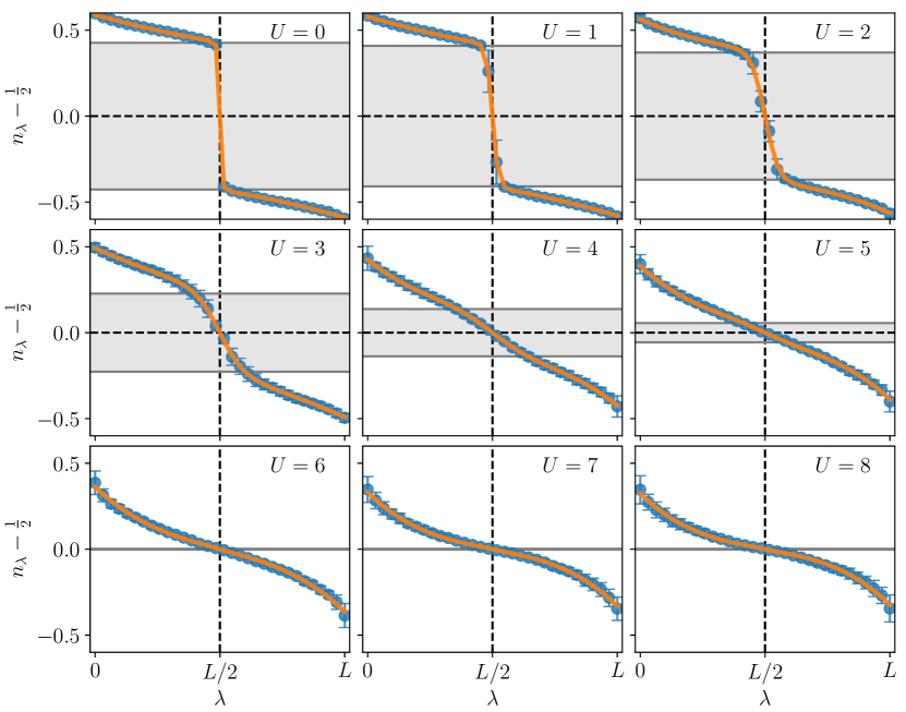
Figure S5: Eigenvalues of the density matrix $n_{\lambda}$ as a function of $\lambda$. Different panels corresponds to different values of $U$ as indicated. Blue dots are the values obtained from HFDS for $L=32$ sites, averaged over twenty disorder realizations. The orange curves are the fit to the functional form in Eq. S10. The dashed vertical line is centered at the Fermi level. The dashed horizontal line is for visual reference at $n_{\lambda}-1/2=0$. The shaded grey area represents the amplitude of the sigmoid in the fitting function (fitting parameter $a$), which corresponds to the quasi-particle weight $Z$.

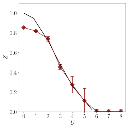
Figure S6: Quasi-particle weight $Z$ as a function of $U$. Maroon diamonds are the values obtained from HFDS for $L=32$, obtained from the fittings shown in Fig. S5 (fitting parameter $a$ in Eq. S10). The error bars correspond to the fitting error for the parameter $a$. The black solid line is the DMFT result in the $L\rightarrow\infty$ limit.

.6 Quasi-particle weight

The Mott transition may also be characterized by the quasi-particle weight $Z$. It can be obtained from the density matrix:

$$\rho_{ij}=\frac{1}{2}\sum_{\sigma}\langle c^{\dagger}_{i\sigma}c_{j\sigma}\rangle.$$ (S9)

We compute $\rho_{ij}$ for a given disorder realization and obtain its eigenvalues $n_{\lambda}$. The eigenvalues are averaged over disorder realizations. Fig. S5 shows $\overline{n_{\lambda}}$ for a system with $L=32$ sites obtained from HFDS. At small $U$ we observe that some of the values of $\overline{n_{\lambda}}$ are outside the allowed values of $\overline{n_{\lambda}}\in[0,1]$. We attribute this discrepancy to the statistical error coming from the Monte Carlo estimation of $\rho_{ij}$, which is then propagated in the diagonalization procedure of the density matrix. Likewise, we also observe that at $U=0$, $\overline{n_{\lambda}}$ is not a perfect step function. We again attribute this discrepancy to the statistical error in the calculation of $\rho_{ij}$ propagating in the diagonalization procedure.

The quasi-particle weight $Z$ is defined as the discontinuity of $n_{\lambda}$ at the Fermi level, which in this case corresponds to $\lambda=L/2$. Finite-size effects “soften” the discontinuity in $n_{\lambda}$ (see Fig. S5) and therefore, the difference $n_{L/2-1}-n_{L/2+1}$ does not provide an accurate estimate for $Z$.

Alternative, the amplitude of smeared out jump in $\overline{n_{\lambda}}$ can be captured by fitting the spectra of the density matrices in Fig. S5 to the functional form:

$$f(\lambda)=a\cdot\left(\frac{1}{1+e^{b\cdot(\lambda-L/2)}}-\frac{1}{2}\right)-c\cdot\lambda-d\cdot\lambda^{3},$$ (S10)

where $a$, $b$, $c$ and $d$ are fitting parameters. The term proportional to $a$ is a sigmoid function representing the smeared out jump, of amplitude $a$ and width inversely proportional to $b$. Thus, the value of $Z$ can be obtained directly from the value of the fitting parameter $a$. The linear and cubic terms in $f(\lambda)$ are included to fit the other features in the density-matrix spectrum observed in Fig. S5. Fig. S5 shows that the proposed functional form in Eq. S10 provides a very accurate fit to the computed values of $\overline{n_{\lambda}}$ from HFDS.

The quasi-particle weight $Z$ extracted from the fits in Fig. S5 is shown in Fig. S6. The DMFT value for $Z$ in the $L\rightarrow\infty$ limit is also included for reference. For $U>1$ the agreement between the HFDS and DMFT value for $Z$ is remarkable. The vanishing of $Z$ for $U\approx 5-6$ clearly marks the metal to Mott insulator transition. This observation clearly shows that the HFDS are capable of accurately describing many-body phenomena to a large degree of accuracy. The discrepancy in the value of $Z$ between DMFT and HFDS at $U=0$ and $U=1$ are a direct consequence of the statistical errors in the computation of the matrix elements of the density matrix, that propagate though the diagonalization procedure, as mentioned above.

.7 Finite-size extrapolation to infinite system size

Due to computational limitations, we perform the DMRG and HFDS calculations with systems of finite size $L$. The collected results for various values of $L$ can then be used to obtained extrapolated results at $L\rightarrow\infty$, as shown in Figure 3. Here, we detail how such extrapolations are performed.

We assume that the dependence on the system size of the quantities of interest follows the equation

$$f(L)=A/L^{b}+f(L\rightarrow\infty),$$ (S11)

where the extrapolated quantity of interest is $f(L\rightarrow\infty)$. In the case of the ground state energy and double occupancy, we first perform a fit of the HFDS data obtained in the metallic regime at $U=0$ with equation S11 and leave all the fit parameters free. This yielded the exponent $b=1.187$ for the energy and $b=2.480$ for the double occupancy. We then perform a second fit in the insulating regime ($U=6$ for the energy, and $U=8$ for the double occupancy), from which we obtain the exponents $b=0.699$ for the energy and $b=1.631$ for the double occupancy. Next, we fix the value of $b$ to the values detailed above in the fit function S11 and perform the fits for the energy and the double occupancy at all values of $U$. The results for the extrapolated quantities at $L\rightarrow\infty$ are shown in panels (b) and (d) of Figure S7. Ultimately, the choice of the exponent does not change significantly the qualitative and quantitative behavior of the extrapolated quantities.

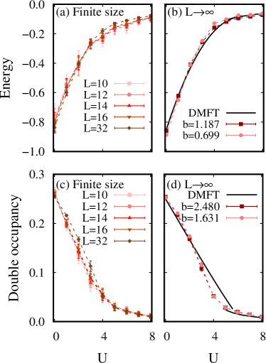
Figure S7: Finite-size scaling of the ground state energy and double occupancy as a function of the Hubbard interaction strength $U$ from HFDS calculations. Panels (a) and (c) show the finite-size results of the energy and double occupancy respectively, for system sizes $L=10,~{}12,~{}14,~{}16$ and $32$. Panels (b) and (d) show the extrapolations to infinite dimensions $L\rightarrow\infty$ using the formula $f(L)=A/L^{b}+f(L\rightarrow\infty)$, where the exponent $b$ takes the values specified in the figures.

In the case of the energy gap, we manually choose the value of the exponent $b=1.65$ as it yields relatively smooth results at all values of $U$ for both the HFDS and DMRG calculations.