On Optimal Control at the Onset of a New Viral Outbreak

Abstract

An optimal control problem for the early stage of an infectious disease outbreak is considered. At that stage, control is often limited to non-medical interventions like social distancing and other behavioral changes. We show that the running cost of control satisfying mild, problem-specific, conditions generates an optimal control strategy that stays inside its admissible set for the entire duration of the study period $[0,T]$. For the optimal control problem, restricted by SIR compartmental model of disease transmission, we prove that the optimal control strategy, $u(t)$, may be growing until some moment $\bar{t}\in[0,T)$. However, for any $t\in[\bar{t},T]$, the function $u(t)$ will decline as $t$ approaches $T$, which may cause the number of newly infected people to increase. So, the window from $0$ to $\bar{t}$ is the time for public health officials to prepare alternative mitigation measures, such as vaccines, testing, antiviral medications, and others. Our theoretical findings are illustrated with numerical examples showing optimal control strategies for various cost functions and weights. Simulation results provide a comprehensive demonstration of the effects of control on the epidemic spread and mitigation expenses, which can serve as invaluable references for public health officials.

Key Words Epidemiology, compartmental model, transmission dynamic, optimal control.

1 Introduction

The circulation of infectious diseases, such as COVID-19, is shaped by multiple parameters including environmental factors [33], immunity patterns [22], superspreading events [20], control interventions [28], and behavior changes [29]. These factors impact the early growth dynamics [31] and the basic reproduction number [21], which quantifies the number of secondary cases per primary case in a completely susceptible population.

Since the first COVID-19 case was detected in December 2019, the disease spread rapidly causing a worldwide pandemic. While some infected people experience only mild or moderate symptoms, others can get seriously ill and require immediate medical intervention [8]. Among high risk individuals are elderly people and those with underlying health conditions such as cancer, diabetes, chronic respiratory disease, and others [9]. As of November 2, 2023, there have been 771,679,618 confirmed cases of COVID-19, including 6,977,023 deaths [24]. Important factors contributing to the alarming rise in COVID‑19 cases at the early stage of the pandemic were high reproduction number, a large number of ”silent spreaders” (especially among young people), and a relatively long incubation period [10]. In the absence of vaccines and antiviral treatments in late 2019 and early 2020 [23], mitigation measures such as social distancing (including full or partial lockdowns), restrictions on travel and mass gatherings, isolation and quarantine of confirmed cases, change from in-person to online education, and other similar tools emerged as the key ways of control and prevention [2, 11]. While these measures proved to be effective in a short-term, they are hard to sustain in a long run due to their negative impact on mental health coupled with high social and economic cost. Hence, since the start of COVID-19, balancing pros and cons of early non-medical interventions has come to the forefront (not only to contain COVID-19, but also to prepare for future epidemic outbreaks) [13, 3, 32, 12, 1, 27, 30, 34, 7, 26, 25, 4].

In this paper, we consider an optimal control problem for SIR compartmental model (Susceptible $\rightarrow$ Infectious $\rightarrow$ Removed) of early disease transmission. We design a running cost of control with mild, practically justified, conditions that give rise to the optimal control strategy, $u(t)$, which stays inside its admissible set for the entire duration of the study period, $[0,T]$. Our theoretical analysis indicates that at the early stage of an outbreak, the optimal control strategy, $u(t)$, may be growing until some moment $\bar{t}\in[0,T)$. However, for any $t\in[\bar{t},T]$, the function $u(t)$ will decline as $t$ approaches $T$, which may cause the number of newly infected people to increase. So, the window from $0$ to $\bar{t}$ is the time for public health officials to prepare alternative mitigation measures, such as vaccines, testing, antiviral medications, and others. Our theoretical findings are illustrated with important numerical examples showing optimal control strategies for various cost parameters. To learn the optimal control function $u(t)$, we employed a deep learning based numerical algorithm, where $u(t)$ is parameterized as a deep neural network (DNN). The implementation, training and testing of all methods were conducted in Python 3.9.6 with PyTorch 2.1.0 and Torchdiffeq 0.2.3.

2 A Strategy for Early Intervention

At the onset of an emerging epidemic, in the absence of a vaccine and antivirals [23], the transmission of individuals between different stages of infection is often described by a classical SIR (Susceptible $\rightarrow$ Infectious $\rightarrow$ Removed) compartmental model [14, 17]. For this early and relatively short phase, it is reasonable to infer that natural birth and death balance one another and, therefore, can be omitted. With the disease death rate varying between age and risk groups and being hard to estimate early on, the removed class is assumed to combine recovered and deceased people. Finally, due to the fast dynamic of the initial pre-vaccination stage, we suppose that recovered individuals develop at least a short-term immunity and don’t move back to the susceptible class until the end of the study period. Under these assumptions, the SIR (Susceptible $\rightarrow$ Infectious $\rightarrow$ Removed/Immune $+$ Deceased) model is given by the following system of ordinary differential equations:

$$\dfrac{d\mathcal{S}}{dt} =-\beta\dfrac{\mathcal{S}(t)\mathcal{I}(t)}{N}$$

$$\dfrac{d\mathcal{I}}{dt} =\beta\dfrac{\mathcal{S}(t)\mathcal{I}(t)}{N}-\gamma\mathcal{I}(t)$$ (2.1)

$$\dfrac{d\mathcal{R}}{dt} =\gamma\mathcal{I}(t)$$

The primary goal of our study is to look at possible control strategies that can be effectively introduced at the early ascending stage of an outbreak before more robust mitigation measures, such as vaccines and viral medications, become available. The most common early mitigation measures, which were broadly used during the recent COVID-19 pandemic, include physical distancing, enhanced personal hygiene, mask wearing, awareness, and others. Their primary goal is to ”flatten the curve”, that is, to reduce the daily number of new infections and, as the result, to reduce the number of virus-related deaths. The SIR model with enforced control, $u=u(t)$, and normalized dependent variables, $S(t):=\dfrac{\mathcal{S}(t)}{N}$, $I(t):=\dfrac{\mathcal{I}(t)}{N}$, and $R(t):=\dfrac{\mathcal{R}(t)}{N}$, takes the form $\frac{d{\bf x}}{dt}=f({\bf x},u)$, where

$$f_{1}({\bf x},u) :=-\beta(1-u(t))S(t)I(t)$$

$$f_{2}({\bf x},u) :=\beta(1-u(t))S(t)I(t)-\gamma I(t)$$ (2.2)

$$f_{3}({\bf x},u) :=\gamma I(t),$$

and ${\bf x}=[S,I,R]^{\top}$. In the above, the admissible set for the control function, $u=u(t)$, is assumed to be

$$\mathcal{U}=\left\{u\in\mathcal{L}^{1}[0,T],\quad 0\leq u(t)<1\right\}.$$

As we show in Lemma 3.2 below, one can design a running cost of $u(t)$ with mild, practically justified, conditions such that the optimal control $0\leq u(t)<1$ is guaranteed for all time $t\in[0,T]$. Therefore, we can assume that the admissible set $\mathcal{U}$ has no explicit constraint on the range of $u(t)$ hereafter. Further, it follows from (2) that

$$\dfrac{d\mathcal{I}}{dt} =\left(\frac{\beta}{\gamma}\,(1-u(t))S(t)-1\right)\gamma I(t),$$ (2.3)

where $\beta/\gamma$ is the basic reproduction number. Clearly, if $\beta S(0)/\gamma<1$, then the virus is contained (even though it can still benefit from mitigation measures that would further reduce the daily number of new infections). It also implies that an obvious way of controlling the disease, should $\beta S(0)/\gamma$ be greater than $1$, is to choose $u(t)$ such that $\beta S(t)(1-u(t))/\gamma\ll 1$. That is, $1>u(t)\gg 1-\frac{\gamma}{S(t)\beta}$. However, all things considered, if the basic reproduction number, $\beta/\gamma$, is large, this kind of control may not be feasible. Indeed, while the right interventions at the onset of the disease save lives and protect the health of the population, they come with social, psychological, and economic costs. Therefore, policymakers have a difficult task of balancing the benefits to public health and the negative outcomes of their preventive measures. Mathematically, this comes down to solving the optimal control problem, where the main goal is to reduce the daily number of new infections, $\beta(1-u(t))S(t)I(t)$, while also minimizing the cost of preventive measures, $\lambda\,c(u(t))$. This gives rise to the following objective functional:

$$J({\bf x}(t),u(t)):=\int_{0}^{T}\biggl{\{}(\beta(1-u(t))S(t)I(t)+\lambda\,c(u(t))\biggr{\}}\,dt,\quad\lambda>0.$$

According to (2), this $J({\bf x}(t),u(t))$ can be written as

$$J({\bf x}(t),u(t))=S(0)-S(T)+\lambda\,\int_{0}^{T}c(u(t))\,dt,\quad\lambda>0.$$ (2.4)

Thus, our goal is to minimize the sum of the terminal cost, $h({\bf x}(T)):=S(0)-S(T)$, which is the cumulative number of cases during the early phase of the outbreak, i.e., from $t=0$ to $t=T$, and the stage cost, $L({\bf x}(t),u(t)):=\lambda\,\int_{0}^{T}c(u(t))\,dt$ (that does not depend on ${\bf x}$ in our case). In other words, for $\lambda>0$,

$$\min_{u\in\mathcal{U}}J({\bf x}(t),u(t)):=h({\bf x}(T))+L({\bf x}(t),u(t))=S(0)-S(T)+\lambda\,\int_{0}^{T}c(u(t))\,dt,$$ (2.5)

subject to controlled SIR model (2). The corresponding Hamiltonian takes the form

$$H({\bf x}(t),u(t),{\bf p}(t)) :=\lambda\,c(u(t))+{\bf p}^{\top}(t)f({\bf x}(t),u(t))=\lambda\,c(u(t))-p_{1}(t)\beta(1-u(t))S(t)I(t)$$

$$+p_{2}(t)(\beta(1-u(t))S(t)I(t)-\gamma I(t))+p_{3}(t)\gamma I(t),$$ (2.6)

where ${\bf p}=[p_{1},p_{2},p_{3}]^{\top}$. From (2.4), one can see that the choice of $c(u(t))$ in $J({\bf x}(t),u(t))$ has a major impact on the resulting control strategy. It is important to define $c(u(t))$ in such a way that the optimal solution, $u=u(t)$, would naturally take values between $0$ and $1$. In other words, it should never be a feasible strategy for $u=u(t)$ to become negative, and the cost of control, $c(u(t))$, should get extremely high as $u(t)$ approaches $1$ (unless the regularization parameter, $\lambda$, is very small).

For various epidemic models, a very common choice of $c(u(t))$ was $c(u(t))=u^{2}(t)$ [3, 32]. This function has some very attractive features since, with this choice of the cost, $\frac{\partial H}{\partial u}({\bf x}(t),u(t),{\bf p}(t))$ is linear in $u$. This gives rise to a forward–backward sweep numerical algorithm for the approximation of $u=u(t)$ [19]. However, as indicated in [3, 32], there are also some drawbacks of using $c(u(t))=u^{2}(t)$. Indeed, since this function has a finite penalty at $u(t)=1$, an explicit constraint $u(t)\in[0,1]$ must be enforced, which often leads to $u(t)$ slipping into some local minimum. Without this constraint, it is easy to get $u(t)>1$ (especially for small values of $\lambda$), which results in unrealistic strategy with $S^{\prime}(t)>0$. For this reason, in our numerical study (see Section 5 below), we employ and compare $4$ different cost functions

$$c_{1}(u)=-\ln(1-u^{2}),\,\,c_{2}(u)=-u\ln(1-u),\,\,c_{3}(u)=-(u+\ln(1-u)),\,\,\mbox{and}\,\,c_{4}(u)=u^{2}.$$

All these functions, except for $c_{4}(u)$, have infinite penalty at $u(t)=1$.

In the next section, we study some basic, yet important, properties of optimal control strategies based on the objective functional (2.4).

3 Properties of Optimal Control

The first order necessary condition for the optimality of $u(t)$, known as Pontryagin’s Minimum Principle, states the following.

Theorem 3.1 [19, 5, 16, 18]. For a given initial condition ${\bf x}(0)={\bf x}_{0}$, let $u(t)\in\mathcal{U}$ be an optimal control trajectory with the associated state variable ${\bf x}(t)$ for the system $\frac{d{\bf x}}{dt}=f({\bf x},u)$ and the objective functional $J({\bf x}(t),u(t)):=h({\bf x}(T))+L({\bf x}(t),u(t))$. Then for the Hamiltonian $H({\bf x}(t),u(t),{\bf p}(t)):=L({\bf x}(t),u(t))+{\bf p}^{\top}(t)f({\bf x}(t),u(t))$, there exists a trajectory ${\bf p}(t)$ such that

$$\dot{\bf p}^{\top}(t) =-\frac{\partial H({\bf x},u,{\bf p})}{\partial{\bf x}}\biggl{|}_{{\bf x}(t),u(t),{\bf p}(t)},\quad{\bf p}^{\top}(T)=\frac{dh({\bf x})}{d{\bf x}}\biggl{|}_{{\bf x}(T)}$$ (3.1)

$$u(t) =\mbox{argmin}_{v\in\mathbb{R}}\hskip 5.69046ptH({\bf x}(t),v,{\bf p}(t)),\quad\forall\,t\in[0,T].$$ (3.2)

Based on Pontryagin’s Minimum Principle we prove the following lemma.

Lemma 3.2. Let $u(t)$ be an optimal control trajectory with ${\bf x}(t)$ satisfying $\frac{d{\bf x}}{dt}=f({\bf x},u)$ defined in (2). Let assumptions of Theorem 3.1 be fulfilled with $L({\bf x}(t),u(t)):=\lambda\,c(u(t))$, $h({\bf x}(T)):=S(0)-S(T)$, and $c=c(u)$ be twice continuously differentiable in its domain containing $[0,1)$, with $\frac{d^{2}c}{du^{2}}>0$, $c(0)=0$, $c^{\prime}(u)>0$ for $u\geq 0$, $c^{\prime}(u)<0$ for $u<0$, and $\lim_{u\to 1^{-}}c(u)=\infty$. Then $u$, the global minimum of $H$, is guaranteed to be in $[0,1)$ pointwisely.

Proof. We claim that (3.2) is indeed equivalent to $u(t)=\mbox{argmin}_{v\in[0,1)}\hskip 5.69046ptH({\bf x}(t),v,{\bf p}(t))$ for all $t\in[0,T].$ To see this, note that by (2), $\frac{\partial^{2}H}{\partial u^{2}}=\lambda\frac{d^{2}c}{du^{2}}$. Therefore, since $\frac{d^{2}c}{du^{2}}>0$, we conclude that $H$ has a unique global minimum with respect to $u$. Let us show that $u$, the global minimum of $H$, is guaranteed to be in $[0,1)$. By the properties of $c$, the Hamiltonian $H$ tends to $+\infty$ as $u\to 1^{-}$, which prevents any $u\geq 1$ from being the optimal of $H$ at any time $t$. On the other hand, the optimality criteria (3.2) leads to

$$\frac{\partial H}{\partial u}=\lambda\frac{dc}{du}+{\bf p}^{\top}\frac{\partial f({\bf x},u)}{\partial u}=\lambda\frac{dc}{du}+\beta\,(p_{1}-p_{2})SI=0,$$ (3.3)

which, together with (3.1), implies that $u(t)$ is differentiable (and, therefore, continuous). Suppose there is $u(t)\leq-\delta<0$ for some $\delta>0$ and $t\in[0,T]$. Then by the continuity of $u=u(t)$ and $c=c(u)$, there exist $\epsilon>0$ and $t_{1}<t_{2}$ such that $c(u(t))\geq\epsilon$ for all $t\in[t_{1},t_{2}]\subset[0,T]$. Then we define $\hat{u}$ such that $\hat{u}(t)=u(t)$ for $t\notin[t_{1},t_{2}]$ and $0$ otherwise. Therefore

$$\int_{t_{1}}^{t_{2}}(c(\hat{u}(t))-c(u(t)))dt=-\int_{t_{1}}^{t_{2}}c(u(t))dt\leq-\epsilon(t_{2}-t_{1})<0.$$

This means that control $u$ incurs larger running cost than $\hat{u}$. Further, we conclude that $1-\hat{u}(t)=1<1+\delta\leq 1-u(t)$ for all $t\in[t_{1},t_{2}]$, and therefore $u(t)$ results in faster decay of $S$ and thus larger terminal cost $S(0)-S(T)$. In summary, we have

$$J^{*}\leq J(\hat{\mathbf{x}},\hat{u})<J(\mathbf{x},u),$$

where $J^{*}$ is the optimal control cost and $\hat{\mathbf{x}}$ is the dynamics obtained by following the control $\hat{u}$. However, this contradicts to the fact that $u$ is the global optimal solution. Hence the global minimum, $u$, is in $[0,1)$. This allows us to drop the constraint $\mathcal{U}$ and directly work on the critical point of $H$ in (3.2).                                                                                               $\Box$

We now prove the main result of this section, Theorem 3.3.

Theorem 3.3. Let $u(t)$ be an optimal control trajectory with the associated state trajectory ${\bf x}(t)$ for the system $\frac{d{\bf x}}{dt}=f({\bf x},u)$ defined in (2). Let the assumptions of Theorem 3.1 and Lemma 3.2 be fulfilled. Then

$$\frac{du}{dt}=\frac{\beta\,\gamma\,S(t)I(t)}{\lambda\,\frac{d^{2}c}{du^{2}}(t)}\,\left\{-1+\lambda\,\int_{t}^{T}\frac{\frac{dc}{du}(\tau)(1-u(\tau))}{S(\tau)}\,d\tau\right\},$$ (3.4)

that is, there is $\bar{t}\in[0,T)$ such that for any $t\in[\bar{t},T]$, the derivative, $\dfrac{du}{dt}$, becomes negative and the optimal trajectory, $u(t)$, decreases as $t$ approaches $T$ (except for special cases when $S(t)$ and/or $I(t)$ are equal to zero).

Proof. To examine the behavior of the optimal control function, $u(t)$, we differentiate identity (3.3) with respect to time variable, $t$. This yields,

$$\lambda\frac{d^{2}c}{du^{2}}\,\frac{du}{dt}+\beta\,(\dot{p_{1}}-\dot{p_{2}})SI+\beta\,(p_{1}-p_{2})(\dot{S}I+S\dot{I})=0,$$

which gives us the rate of change for the control function, $u(t)$, $t\in[0,T]$, as follows

$$\frac{du}{dt}=\frac{\beta}{\lambda}\,\frac{(\dot{p_{2}}-\dot{p_{1}})SI+(p_{2}-p_{1})(\dot{S}I+S\dot{I})}{\frac{d^{2}c}{du^{2}}}.$$ (3.5)

According to (2.4), the stage cost of the control, $\lambda\,\int_{0}^{T}c(u(t))\,dt,$ does not depend on ${\bf x}$. Hence

$$\frac{\partial H({\bf x},u,{\bf p})}{\partial{\bf x}}={\bf p}^{\top}\frac{\partial f({\bf x},u)}{\partial{\bf x}}=[p_{1},p_{2},p_{3}]\begin{bmatrix}\dfrac{\partial f_{1}}{\partial S}&\dfrac{\partial f_{1}}{\partial I}&\dfrac{\partial f_{1}}{\partial R}\\ \dfrac{\partial f_{2}}{\partial S}&\dfrac{\partial f_{2}}{\partial I}&\dfrac{\partial f_{2}}{\partial R}\\ \dfrac{\partial f_{3}}{\partial S}&\dfrac{\partial f_{3}}{\partial I}&\dfrac{\partial f_{3}}{\partial R}\end{bmatrix}.$$

This implies that costate equations (3.1) with terminal conditions at $t=T$ take the form

$$\dot{{{\bf p}}}^{\top}=-\left[\sum_{k=1}^{3}p_{k}\dfrac{\partial f_{k}}{\partial S},\sum_{k=1}^{3}p_{k}\dfrac{\partial f_{k}}{\partial I},\sum_{k=1}^{3}p_{k}\dfrac{\partial f_{k}}{\partial R}\right]\quad\mbox{and}\quad{\bf p}^{\top}(T)=\frac{dh({\bf x})}{d{\bf x}}\biggl{|}_{{\bf x}(T)}=[-1,0,0].$$

Taking into consideration (2), one has $\,p_{3}(t)=0\,$ and

$$\begin{cases}\dot{p_{1}}=-\beta\,(p_{2}-p_{1})(1-u)I\\ \dot{p_{2}}=-\beta\,(p_{2}-p_{1})(1-u)S+\gamma\,p_{2}\\ p_{1}(T)=-1,\,\,p_{2}(T)=0.\end{cases}$$ (3.6)

From system (3.6), one concludes

$$\dot{p_{2}}-\dot{p_{1}}=\beta\,(p_{2}-p_{1})(1-u)(I-S)+\gamma\,p_{2}.$$ (3.7)

Combining (2) and (3.7), one can rewrite the numerator in (3.5) as follows

$$(\dot{p_{2}}-\dot{p_{1}})SI+(p_{2}-p_{1})(\dot{S}I+S\dot{I}) =\beta\,(p_{2}-p_{1})(1-u)(I-S)SI+\gamma p_{2}SI$$

$$+(p_{2}-p_{1})\bigl{\{}-\beta(1-u)SI^{2}+\beta(1-u)S^{2}I-\gamma SI)\bigr{\}}$$

$$=\bigl{\{}\beta\,(p_{2}-p_{1})(1-u)(I-S)+\gamma p_{2}+\beta\,(p_{2}-p_{1})$$

$$\times(1-u)(S-I)-\gamma(p_{2}-p_{1})\bigr{\}}SI=\gamma p_{1}SI.$$

Together with (3.5), this yields

$$\frac{du}{dt}=\frac{\beta\,\gamma\,S(t)I(t)}{\lambda\,\frac{d^{2}c}{du^{2}}(t)}\,p_{1}(t).$$ (3.8)

Thus, if the assumptions of Theorem 3.1 are met and $\frac{d^{2}c}{du^{2}}(t)>0$, then the optimal control strategy, $u(t)$, has the same sign as $p_{1}(t)$. From the optimality condition (3.3),

$$\lambda\,\frac{dc}{du}(1-u)+\beta\,(p_{1}-p_{2})(1-u)SI=0.$$ (3.9)

By substituting this into costate system (3.6), one can uncouple the equations for $p_{1}(t)$ and $p_{2}(t)$ to obtain

$$\begin{cases}\dot{p_{1}}=-\frac{\lambda\,\frac{dc}{du}(1-u)}{S}\\ \dot{p_{2}}=-\frac{\lambda\,\frac{dc}{du}(1-u)}{I}+\gamma\,p_{2}\\ p_{1}(T)=-1,\,\,p_{2}(T)=0.\end{cases}$$ (3.10)

The first equation in (3.10) along with its boundary condition imply that

$$p_{1}(t)=-1+\lambda\,\int_{t}^{T}\frac{\frac{dc}{du}(\tau)(1-u(\tau))}{S(\tau)}\,d\tau.$$ (3.11)

This yields identity (3.4). Clearly, the cost of any realistic preventive measure, $c(u)$, must go up as $u$ changes from $0$ to $1$. Therefore, $\frac{dc}{du}$ should be greater than zero for any admissible control function, which means $\lambda\,\int_{t}^{T}\frac{\frac{dc}{du}(\tau)(1-u(\tau))}{S(\tau)}\,d\tau>0$ for any $t\in[0,T)$. This indicates that the optimal control strategy, $u(t)$, may be growing until some moment $\bar{t}\in[0,T)$. However, according to (3.8) and (3.11), for any $t\in[\bar{t},T]$, the derivative, $\dfrac{du}{dt}$, becomes negative and $u(t)$ decreases as $t$ approaches $T$ (unless $S(t)$ and/or $I(t)$ are equal to zero). This completes the proof.                                                                                                                         $\Box$

Remark 3.4 Following the decline in $u(t)$, the number of newly infected people may increase. So, the window from $0$ to $\bar{t}$ is the time for public health officials to prepare alternative mitigation measures, such as vaccines, testing, antiviral medications, and others. The impact of $u(t)$ scaling down towards the end of the early stage will depend on the cost, $\lambda$. If the cost of control is relatively high (see Figures 3 and 4 in Section 5), then the decline in $u(t)$ for $t\geq\bar{t}$ can be substantial, which will result in a notable surge in the daily number of infected individuals, $\mathcal{I}(t)$, for $t\geq\bar{t}$. On the other hand, if the cost, $\lambda$, is low (as in Figure 5), then by the time $t=\bar{t}$ the epidemic is effectively under control. Hence, as it follows from (3.8) and (3.11), the decline in $u(t)$ for $t\geq\bar{t}$ is negligible and the daily number of infected people, $\mathcal{I}(t)$, remains very low for $t\geq\bar{t}$.

Note that cost functional (2.4) aims to minimize the cumulative number of cases during the early phase of the outbreak, i.e., for $t\in[0,T]$. However, it does not guarantee that on any given day, the number of infected individuals in the optimally controlled environment is less than the number of infected individuals in the same environment but with no control. As our experiments below illustrate, when the cost of control, $\lambda$, is relatively high, towards the end of the study period in a controlled environment the daily number of infected humans, $I(t)$, can potentially bypass the corresponding $I(t)$ in the environment with no control (see Figures 3 and 4 in Section 5). The objective functional (2.4) is set to minimize the cumulative number of infections, $S(0)-S(T)$, while keeping the negative impact of mitigation measures at bay. This is achieved, for the most part, by reducing the daily number of new infections but also, apparently, by delaying some infections. On the bright side, $I(t)$ in the controlled environments gets bigger than $I(t)$ in the uncontrolled case only when $t$ is approaching $T$. It is reasonable to assume that at this time additional intervention measures become available that will gradually replace the initial set of controls.

In the running cost, rather than minimizing the daily number of new infections, one can also minimize the daily number of infected individuals. This gives rise to the following cost functional

$$J({\bf x}(t),u(t)):=\int_{0}^{T}\bigl{\{}I(t)+\lambda\,c(u(t))\bigr{\}}\,dt=\frac{R(T)-R(0)}{\gamma}+\lambda\,\int_{0}^{T}c(u(t))\,dt.$$ (3.12)

That is, instead of maximizing $S(T)$, this functional aims to minimize $R(T)$. Using the similar argument as above, one arrives at the following expression for $\frac{du}{dt}$:

$$\frac{du}{dt}=\frac{\beta\,S(t)I(t)}{\lambda\,\frac{d^{2}c}{du^{2}}(t)}\,\left\{-1+\gamma\lambda\,\int_{t}^{T}\frac{\frac{dc}{du}(\tau)(1-u(\tau))}{S(\tau)}\,d\tau\right\},$$ (3.13)

which indicates that this optimal control strategy, $u(t)$, will also be decreasing starting with some point $\hat{t}\in[0,T)$.

4 Numerical Algorithm for Learning Control

To learn the control function, $u:\,[0,T]\to\mathbb{R}$, which is guaranteed to take values in $[0,1)$ according to Lemma 3.2 above, we employ a deep learning based numerical algorithm. This algorithm can be easily modified to the case of vector-valued controls. At the first step, we parameterize $u$ as a deep neural network (DNN), denoted by $u_{\theta}$, with parameters $\theta\in\mathbb{R}^{m}$. In our experiments, we chose a simple fully connected network with both input and output layer dimension 1 (because in our setting, the input is time $t\in[0,T]$ and the output is a scalar). We set $u_{\theta}$ to have 4 hidden layers and each layer is of size $10$. All trainable parameters are collectively denoted by $\theta$. Introduce the notation

$$\ell(\theta):=J(\mathbf{x}(t),u_{\theta}(t))),$$

where $J$ is defined in (2.4) and $\mathbf{x}$ follows the dynamics (2) with the given initial state $\mathbf{x}(0)=(S(0),I(0),R(0))$. To find the optimal $u_{\theta}$, we essentially need to compute $\nabla_{\theta}\ell(\theta)$ for any $\theta$ and apply the gradient descent to update $\theta$. In our algorithm, we employ the neural ordinary differential equation (NODE) method [6] which computes $\nabla_{\theta}\ell(\theta)$ in the following way. First, with the given $\theta$, one solves the ODE forward in time:

$$\dot{\mathbf{x}}(t)=f(\mathbf{x}(t),u_{\theta}(t)),\quad t\in[0,T],$$ (4.1)

with initial value $\mathbf{x}(0)=\mathbf{x}_{0}$ and $f(\mathbf{x},u)$ defined in (2). Second, one solves the augmented adjoint equation backward in time:

$$(\dot{\mathbf{p}}(t),\ \dot{\mathbf{a}}(t))=-(\mathbf{p}(t)\,\partial_{\mathbf{x}}f(\mathbf{x}(t),u_{\theta}(t)),\ \mathbf{p}(t)\,\partial_{u}f(\mathbf{x}(t),u_{\theta}(t))\,\partial_{\theta}u_{\theta}(t)),\quad t\in[0,T],$$ (4.2)

with terminal value $(\mathbf{p}(T),\mathbf{x}(T))=(-\nabla h(\mathbf{x}(T)),\mathbf{0})$. Here $\mathbf{x},\mathbf{p},\mathbf{a}$ are all row vectors at each time $t$. Then it can be shown that $\nabla_{\theta}\ell(\theta)=\mathbf{a}(0)$ [6]. The algorithm is summarized in Algorithm 1 below. The implementation, training and testing were conducted in Python 3.9.6 with PyTorch 2.1.0 and Torchdiffeq 0.2.3.

Algorithm 1 Neural ODE method to solve the optimal control problem of $u$

Cost function $c$ and weight $\lambda>0$. Network structure $u_{\theta}$. Initial guess $\theta$.

Optimal control $u_{\theta}$ with trained $\theta$.

repeat

     Solve $\mathbf{x}$ forward in time using (4.1).

     Solve $(\mathbf{p},\mathbf{a})$ backward in time using (4.2).

     $\theta\leftarrow\theta-\tau\mathbf{a}(0)$.

until converged.

A few details about the performance of Algorithm 1 and our numerical simulations:

• In our experiments, we try $4$ different cost functions, $c=c(u)$. Details and discussion will be given in Section 5;

• The weight, $\lambda$, scales the cost function, $c=c(u)$, and can be critical to the optimal control solution. In Section 5, we conduct empirical study on different values of $\lambda$;

• One can apply any numerical integrator (e.g., Euler, mid-point, Runge-Kutta) to solve (4.1) and (4.2). We used the 4th order Runge-Kutta method (rk4) built in the PyTorch package;

• One can either solve $(\mathbf{p},\mathbf{a})$ as in (4.2) or solve $\mathbf{x}$ jointly backward in time to avoid saving $\mathbf{x}(t)$ obtained forward in (4.1) in the memory;

• In Algorithm 1, one can choose the step size $\tau>0$ and terminate the algorithm after a prescribed number of iterations, $K$. We used Adam [15] with deterministic gradient and set these parameters as $\tau=0.001$ and $K=1,000$ and other parameters as default. The results appear to be stable for values around them;

• Since the control problem is not convex in $(\mathbf{x},u)$, it is not guaranteed that our solution is the global minimizer. This is, unfortunately, a common issue in solving optimal control problems. Nevertheless, in all experiments, the numerical solutions obtained by our method appear to satisfy the constraint $u(t)\in[0,1)$ for all $t\in[0,T]$ and $du(t)/dt<0$ starting with some $\bar{t}\in[0,T)$.

5 Numerical Results and Discussion

In this section, we apply the deep learning based numerical algorithm to the control problem (2.5) subject to controlled SIR model (2) with the following four cost functions:

$$c_{1}(u) =-0.830071\,\ln(1-u^{2})$$

$$c_{2}(u) =-0.672850\,u\ln(1-u)$$

$$c_{3}(u) =-z-\ln(1-u)$$

$$c_{4}(u) =1.424546\,u^{2}.$$

The weight $0.830071$ in $c_{1}$ is chosen to minimize the distance

$$\int_{0}^{1}w(z)|c_{1}(z)-c_{3}(z)|^{2}\,dz,\quad w(z)=\sqrt{1-z^{2}},$$

(the same for $c_{2},c_{4}$). Doing so makes $c_{i}$’s close in the $w$-weighted 2-norm sense. See the comparison of these cost functions in Figure 1.

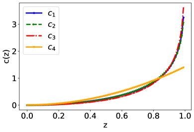
Figure 1: Comparison of different cost functions $c$.

In our experiments, we consider $\lambda$ as $0.1$, $0.05$, $0.01$, and $10^{-7}$. For $\lambda=0.1$, the environment is close to no control as shown in Figure 2, since the penalty on control is weighted highly. All values of $\lambda$ larger than $0.1$ resulted in a similar behavior and hence they were omitted here.

As $\lambda$ gradually decreases, we see that controls start to make impact as they become cheaper to implement. For example, as shown in Figure 3, when $\lambda=0.05$, we observe that $c_{1}(u)$, $c_{2}(u)$, and $c_{3}(u)$ generate similar control strategies that effectively suppress the cumulative number of infected people (or equivalently maximize $S(T)$).

We note that all three controls, $c_{1}(u)$, $c_{2}(u)$, and $c_{3}(u)$, make a considerable positive impact on how the epidemic unfolds. Even though $\mathcal{I}(t)$ in the controlled environment is still growing (see Table 1), the daily number of infected people remains low for a long time. However, as expected from our theoretical analysis, for all three cost functions, $c_{1}(u)$, $c_{2}(u)$, and $c_{3}(u)$, and $\lambda=0.05$, the corresponding control strategies, $u(t)$, begin to decrease after some point.

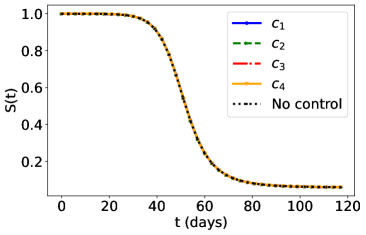
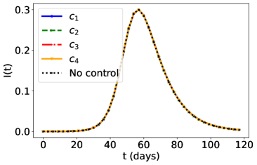
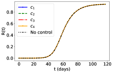
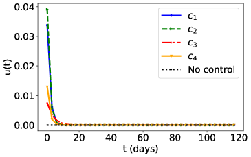
Figure 2: Weight $\lambda=0.1$.

Thus, towards the end of the study period in a controlled environment the daily number of infected humans, $\mathcal{I}(t)$, bypasses the corresponding $\mathcal{I}(t)$ in the environment with no control.

Table 1: Number of infected people $\mathcal{I}(t)$ versus day $t$ for $\lambda=0.05$

Day	No control	$c_{1}$	$c_{2}$	$c_{3}$	$c_{4}$
0	200	200	200	200	200
10	1626	423	423	407	1600
20	12542	889	891	824	12341
30	92164	1856	1882	1660	90714
40	643531	3898	4004	3370	634826
50	2358721	8104	8348	6785	2344806
60	2852657	16674	17093	13546	2858895
70	1722500	34405	35574	27592	1731405
80	834814	69687	72449	57021	839919
90	373748	137590	143188	118394	376160
100	164980	276638	282921	245423	166065
110	71628	567049	572008	479114	72103

As mention in Remark 3.4, the objective functional (2.4) is set to minimize the cumulative number of infections, $\mathcal{S}(0)-\mathcal{S}(T)$, which it does successfully as it is evident from Table 2. This is achieved, for the most part, by reducing the daily number of new infections but also, apparently, by delaying some infections. As one can clearly see from Figure 3 and Tables 1 and 2, the cost of the optimal control strategy, $u(t)$, corresponding to $c_{4}$, is still very high for $\lambda=0.05$, and this control does not defeat the outbreak. The reason for this control being different from $c_{1}(u)$, $c_{2}(u)$, and $c_{3}(u)$ can be understood from Figure 1, which shows that the cost, $c_{4}(u)$, is greater than the cost of all other controls between $u=0.2$ and $u=0.8$.

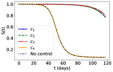
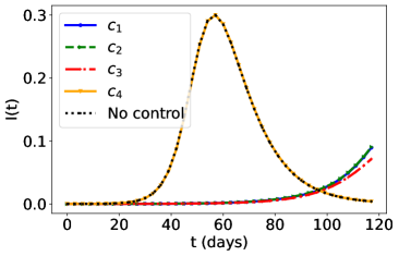
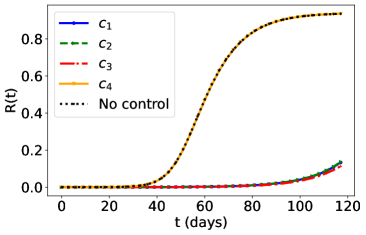
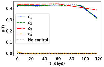
Figure 3: Weight $\lambda=0.05$.

When $\lambda$ reaches $0.01$, the scale on the cost function is small and all optimal control strategies, $u(t)$, corresponding to cost functions $c_{1}(u)$, $c_{2}(u)$, $c_{3}(u)$, and $c_{4}(u)$ appear to suppress infections more aggressively, as illustrated in Figure 4. The actual values of $\mathcal{I}(t)$ are shown in Table 3. The total numbers of infected people up to day $t$, $\mathcal{S}(0)-\mathcal{S}(t)$, for all four control functions, $c_{1}(u)$, $c_{2}(u)$, $c_{3}(u)$, and $c_{4}(u)$, are presented in Table 4.

Table 2: Total number of infected people up to day $t$, $N-\mathcal{S}(t)$, for $\lambda=0.05$

Day	No control	$c_{1}$	$c_{2}$	$c_{3}$	$c_{4}$
0	200	200	200	200	200
10	2339	734	731	709	2303
20	18723	1835	1843	1724	18425
30	138618	4154	4182	3786	136445
40	993903	9034	9212	7991	980029
50	4179153	19132	19626	16404	4146211
60	7574716	39793	40813	33135	7557842
70	8800810	82846	85337	67540	8795738
80	9181982	169453	175482	138477	9180310
90	9316270	339228	352155	285376	9315647
100	9367572	682997	703593	592907	9367317
110	9388987	1389004	1413628	1187340	9388880

As $\lambda$ continues to decrease, we see similar behavior as in Figure 4 except that $u(t)$ become larger and the infections are further suppressed. For example, when $\lambda=10^{-7}$, the cost is very lightly weighted and hence one can impose greater control as shown in Figure 5.

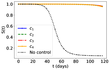
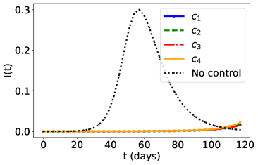
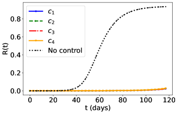
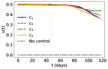
Figure 4: Weight $\lambda=0.01$.

Again, the behavior of $c_{4}(u)$ is different. As mentioned above, this control requires an explicit constraint, $u(t)\in[0,1]$. If not, it is easy to get $u(t)>1$ (especially for small $\lambda$) because it makes $S^{\prime}(t)>0$, which is not realistic. With the constraint enforced, $u(t)$, corresponding to $c_{4}(u)$, is likely slipping into a local minimum.

Table 3: Number of infected people $\mathcal{I}(t)$ versus day $t$ for $\lambda=0.01$

Day	No control	$c_{1}$	$c_{2}$	$c_{3}$	$c_{4}$
0	200	200	200	200	200
10	1626	335	340	333	339
20	12542	559	575	550	567
30	92164	932	973	912	951
40	643531	1563	1660	1522	1599
50	2358721	2616	2829	2542	2649
60	2852657	4380	4818	4245	4431
70	1722500	7447	8269	7155	7587
80	834814	12778	14502	12221	13336
90	373748	22520	26401	21821	25197
100	164980	43921	50317	42319	52546
110	71628	95049	97855	87251	117329

As illustrated in Figure 5, by the time $u(t)$ begins to decrease, the epidemic is effectively under control. Hence, as it follows from (3.8) and (3.11), the decline in $u(t)$ for $t\geq\bar{t}$ is negligible and the daily number of infected people, $\mathcal{I}(t)$, remains very low for $t\geq\bar{t}$.

For all numerical experiments presented in this section, we let the entire population, $N$ be $10^{7}$ people with $\mathcal{I}(0)=200$, $\mathcal{R}(0)=0$, and $\mathcal{S}(0)=N-200$.

Table 4: Total number of infected people up to day $t$, $N-\mathcal{S}(t)$, for $\lambda=0.01$

Day	No control	$c_{1}$	$c_{2}$	$c_{3}$	$c_{4}$
0	200	200	200	200	200
10	2339	604	612	600	615
20	18723	1276	1304	1261	1289
30	138618	2394	2474	2358	2437
40	993903	4287	4485	4189	4369
50	4179153	7424	7899	7250	7554
60	7574716	12685	13704	12335	12865
70	8800810	21705	23742	20996	22079
80	9181982	37149	41310	35740	38214
90	9316270	64362	73392	62132	68915
100	9367572	118524	135484	114391	134473
110	9388987	236989	256274	222679	281497

We use $T=120$, which mimics a 4-months time frame. This value of $T$ allows us to realistically assume that individuals recovered from COVID-19 still have immunity and stay in the removed class, $\mathcal{R}$, for the entire duration of the study period. Furthermore, we take $\beta=0.3$ and $\gamma=0.1$ days^-1, which correspond to the reproduction number, $\mathfrak{R}=3$, and the recovery rate of 10 days.

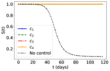
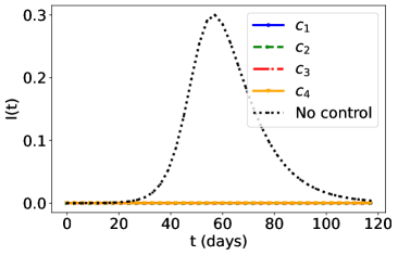
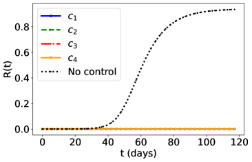
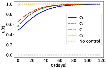
Figure 5: Weight $\lambda=10^{-7}$.

6 Conclusions

In our study, we combine theoretical analysis with rigorous numerical exploration of an optimal control problem for the early stage of an infectious disease outbreak. We design an objective functional aimed at minimizing the cumulative number of cases. The running cost of control, satisfying mild, problem-specific, conditions generates an optimal control strategy, $u(t)$, that is proven to stay inside its admissible set for any $t\in[0,T]$. For the optimal control problem, restricted by SIR compartmental model (Susceptible $\rightarrow$ Infectious $\rightarrow$ Removed) of disease transmission, we show that the optimal control strategy, $u(t)$, may be growing until some moment $\bar{t}\in[0,T)$. However, for any $t\in[\bar{t},T]$, the derivative, $\dfrac{du}{dt}$, becomes negative and $u(t)$ declines as $t$ approaches $T$ possibly causing the number of newly infected people to go up. So, the window from $0$ to $\bar{t}$ is the time for public health officials to prepare alternative mitigation measures, such as vaccines, testing, and antiviral medications, and to plan for the deployment of rescue equipments like ventilators and beds.

The impact of $u(t)$ decreasing towards the end of the early stage depends on the weight, $\lambda$. If $\lambda$ is relatively high, then the decline in $u(t)$ for $t\geq\bar{t}$ may be significant, which can result in a considerable surge in the daily number of infected individuals, $\mathcal{I}(t)$, for $t\geq\bar{t}$. On the other hand, if $\lambda$ is small, then by the time $t=\bar{t}$ the epidemic is effectively under control. Hence, as it follows from (3.8) and (3.11), the decline in $u(t)$ for $t\geq\bar{t}$ is negligible and the daily number of infected people, $\mathcal{I}(t)$, remains very low for $t\geq\bar{t}$.

Our theoretical findings are illustrated with important numerical examples showing optimal control strategies for various cost functions and weights. Simulation results provide a comprehensive demonstration of the effects of control on the epidemic spread and mitigation expenses, which can serve as invaluable references for public health officials. The important next step is to consider the case of vector-valued controls that, on top of early non-medical interventions (such as social distancing, restrictions on travel and mass gatherings, isolation and quarantine of confirmed cases), include treatment with antivirals and the optimal vaccination strategy.

References

- [1] M. Soledad Aronna, Roberto Guglielmi, and Lucas M. Moschen. A model for covid-19 with isolation, quarantine and testing as control measures, 2020.
- [2] Summer Atkins, Mahya Aghaee, Maia Martcheva, and William Hager. Solving singular control problems in mathematical biology using pasa. Computational and Mathematical Population Dynamics, 16(1):412–438, 2023.
- [3] Vijay Pal Bajiya, Sarita Bugalia, Jai Prakash Tripathi, and Maia Martcheva. Deciphering the transmission dynamics of covid-19 in india: optimal control and cost effective analysis. Journal of Biological Dynamics, 16(1):665–712, 2022.
- [4] Marshall N. Barlow M. and Tyson R. Optimal shutdown strategies for covid-19 with economic and mortality costs: British columbia as a case study. Royal Society Open Science, 8:1 – 18, 2021.
- [5] Liming Cai, Xuezhi Li, Necibe Tuncer, Maia Martcheva, and Abid Ali Lashari. Optimal control of a malaria model with asymptomatic class and superinfection. Mathematical Biosciences, 288:94–108, 2017.
- [6] Ricky TQ Chen, Yulia Rubanova, Jesse Bettencourt, and David K Duvenaud. Neural ordinary differential equations. Advances in neural information processing systems, 31, 2018.
- [7] Vincent Denoël, Olivier Bruyère, Gilles Louppe, Fabrice Bureau, Vincent D’orio, Sébastien Fontaine, Laurent Gillet, Michèle Guillaume, Éric Haubruge, Anne-Catherine Lange, et al. Decision-based interactive model to determine re-opening conditions of a large university campus in belgium during the first covid-19 wave. Archives of Public Health, 80(1):1–13, 2022.
- [8] Drugs.com. How do covid-19 symptoms progress and what causes death?, 2022.
- [9] CDC Center for Disease Control and Prevention. People with certain medical conditions, 2023.
- [10] CDC Center for Disease Control and Prevention. Understanding risk, 2023.
- [11] Organisation for Economic Co-operation and Development. Oecd policy responses to coronavirus (covid-19) flattening the covid-19 peak: Containment and mitigation policies, 2023.
- [12] Musadaq A. Hadi and Hazem I. Ali. Control of covid-19 system using a novel nonlinear robust control algorithm. Biomedical Signal Processing and Control, page 102, 2020.
- [13] M. Igoe, R. Casagrandi, M. Gatto, CM. Hoover, L. Mari, CN. Ngonghala, JV. Remais, JN. Sanchirico, SH. Sokolow, S. Lenhart, and G. de Leo. Reframing optimal control problems for infectious disease management in low-income countries. Bull Math Biol, 85(4:31), 2023.
- [14] William Ogilvy Kermack and Anderson G McKendrick. A contribution to the mathematical theory of epidemics. Proceedings of the royal society of london. Series A, Containing papers of a mathematical and physical character, 115(772):700–721, 1927.
- [15] Diederik P. Kingma and Jimmy Ba. Adam: A method for stochastic optimization. In Yoshua Bengio and Yann LeCun, editors, 3rd International Conference on Learning Representations, ICLR 2015, San Diego, CA, USA, May 7-9, 2015, Conference Track Proceedings, 2015.
- [16] D. E. Kirk. Optimal control theory: An introduction. Prentice Hall, 1970.
- [17] Nikolay A Kudryashov, Mikhail A Chmykhov, and Michael Vigdorowitsch. Analytical features of the sir model and their applications to covid-19. Applied Mathematical Modelling, 90:466–473, 2021.
- [18] E. B. Lee and L. Markus. Foundations of optimal control theory. New York: Wiley, 1967.
- [19] S. Lenhart and J.T.Workman. Optimal control applied to biological models. Chapman and Hall/CRC, 2007.
- [20] J. O. Lloyd-Smith, S. J. Schreiber, P. E. Kopp, and W. M. Getz. Superspreading and the effect of individual variation on disease emergence. Nature, 438:355–359, 2005.
- [21] I. Locatelli, B. Trächsel, and V. Rousson. Estimating the basic reproduction number for covid-19 in western europe. PLoS ONE, 16(3):e0248731, 2021.
- [22] M. O’Driscoll, G. Ribeiro Dos Santos, L. Wang, D. A. T. Cummings, A. S. Azman, J. Paireau, A. Fontanet, S. Cauchemez, and H. Salje. Age-specific mortality and immunity patterns of sars-cov-2. Nature, 590:140–145, 2021.
- [23] HHS U.S. Department of Health and Human Services. What are the possible treatment options for covid‑19?, 2023.
- [24] WHO World Health Organization. Who coronavirus (covid-19) dashboard, 2023.
- [25] A David Paltiel, Amy Zheng, and Rochelle P Walensky. Assessment of sars-cov-2 screening strategies to permit the safe reopening of college campuses in the united states. JAMA network open, 3(7):e2016818–e2016818, 2020.
- [26] Jasmina Panovska-Griffiths, Cliff C Kerr, Robyn M Stuart, Dina Mistry, Daniel J Klein, Russell M Viner, and Chris Bonell. Determining the optimal strategy for reopening schools, the impact of test and trace interventions, and the risk of occurrence of a second covid-19 epidemic wave in the uk: a modelling study. The Lancet Child & Adolescent Health, 4(11):817–827, 2020.
- [27] Fernando A. Pazos and Flavia Felicioni. A control approach to the covid-19 disease using a seihrd dynamical model. medRxiv, 2020.
- [28] T. A. Perkins and Guido España. Optimal control of the covid-19 pandemic with non-pharmaceutical interventions. Bulletin of mathematical biology, 82(9):118, 2020.
- [29] Jennifer M. Radin, Giorgio Quer, Edward Ramos, Katie Baca-Motes, Matteo Gadaleta, Eric J. Topol, and Steven R. Steinhubl. Assessment of prolonged physiological and behavioral changes associated with covid-19 infection. JAMA Network Open, 4(7):e2115959–e2115959, 07 2021.
- [30] Jakub Svoboda, Josef Tkadlec, Andreas Pavlogiannis, Krishnendu Chatterjee, and Martin A Nowak. Infection dynamics of covid-19 virus under lockdown and reopening. Scientific reports, 12(1):1–11, 2022.
- [31] B. Szendroi and G. Csanyi. Polynomial epidemics and clustering in contact networks. Proceedings of the Royal Society of London. Series B: Biological Sciences, 5:364–366, 2004.
- [32] Necibe Tuncer, Archana Timsina, Miriam Nuno, Gerardo Chowell, and Maia Martcheva. Parameter identifiability and optimal control of a sars-cov-2 model early in the pandemic. Journal of Biological Dynamics, 16(1):412–438, 2022.
- [33] R. A. Weiss and A.J. McMichael. Social and environmental risk factors in the emergence of infectious diseases. Nature medicine, 10,12:70–6, 2004.
- [34] Pei Yuan, Elena Aruffo, Evgenia Gatov, Yi Tan, Qi Li, Nick Ogden, Sarah Collier, Bouchra Nasri, Iain Moyles, and Huaiping Zhu. School and community reopening during the covid-19 pandemic: A mathematical modelling study. Royal Society Open Science, 9(2):211883, 2022.