Cut-set and Stability Constrained Optimal Power Flow for Resilient Operation During Wildfires

Abstract

Resilient operation of the power system during ongoing wildfires is challenging because of the uncertain ways in which the fires impact the electric power infrastructure (multiple arc-faults, complete melt-down). To address this challenge, we propose a novel cut-set and stability-constrained optimal power flow (OPF) that quickly mitigates both static and dynamic insecurities as wildfires progress through a region. First, a Feasibility Test (FT) algorithm that quickly desaturates overloaded cut-sets to prevent cascading line outages is integrated with the OPF problem. Then, the resulting formulation is combined with a data-driven transient stability analyzer that predicts the correction factors for eliminating dynamic insecurities. The proposed model considers the possibility of generation rescheduling as well as load shed. The results obtained using the IEEE 118-bus system indicate that the proposed approach alleviates vulnerability of the system to wildfires while minimizing operational cost.

I Introduction

In recent years, the prevalence of wildfires has surged, posing monumental challenges for electric power utilities. On one side, they have been blamed for starting devastating wildfires, which have even culminated in some utilities declaring bankruptcy [1]. On the other side, they are expected to maintain secure and stable grid operation in presence of ongoing wildfires to support other critical services. The focus of this paper is on the latter, i.e., ensuring resilient power system operation in presence of active wildfire risks.

An analysis of major wildfire-induced system interruptions has identified cascading outages resulting from overloaded lines, frequent arc-faults, and/or preemptive disconnections as the primary concerns. Overloads occur because the heat from the fires affect the power lines in their vicinities resulting in lowering of the conductor’s current carrying capacity [2]. This lowering may then cause bottlenecks to appear in other parts of the system. The pioneering work on this topic was done by [3]. However, [3] and the papers that cited it, did not consider the impacts of fire-induced faults on dynamic stability of the power system. During the 2016 Blue Cut Fire, as the fire approached a corridor of three 500kV and two 287kV transmission lines, 15 line faults occurred in a short period of time [4]. Other instances of system instabilities caused by fire-induced arc-faults can be found in [5, 6, 7]. Arc-faults caused by wildfires are unique because of their ability to occur multiple times within a few seconds [8]. As such, the impact of such types of repeated faults on the transient stability of the power system must be carefully investigated.

A phasor measurement unit (PMU)-based just-in-time disconnection of overhead lines at the approach of forest fires (to prevent fire-induced arc-faults) was proposed in [9]. However, it required both ends of the lines to be monitored by PMUs. At the same time, preemptively disconnecting lines well in advance and over wide regions to protect them from future arc-faults bears a very high social cost. During the 2019 California fires, preemptive actions by the local utility left more than 2.7 million people without electricity [10]. In summary, during ongoing wildfires, power utilities must continue to operate till the last-minute while also considering static security (to minimize occurrence of overloads) as well as dynamic stability (to minimize impact of frequent arc-faults) of the system.

In this paper, we introduce a novel cut-set and stability-constrained optimal power flow (CSCOPF) formulation to manage active wildfire risks. A cut-set is a set of lines, which if tripped, would create disjoint islands in the network. Therefore, saturated/overloaded cut-sets are the most vulnerable interconnections of the system because they have limited power transfer capability [11]. For ensuring static security, we leverage the Feasibility Test (FT) algorithm developed in [12] to protect the system against overloaded cut-sets. Dynamic security is ensured through a data-driven transient stability constraint prediction (TSCP) algorithm that estimates the required transient stability correction factor (TSCF) while accounting for load and generation uncertainties. The outcomes of the two algorithms are added as constraints to the optimal power flow (OPF) problem. To ensure flexibility in implementation, the security and stability constraints are enforced using generation rescheduling as well as load shedding. A case-study conducted using the IEEE 118-bus system demonstrate that the proposed approach is able to alleviate cascading outages due to static/dynamic insecurities with minimal increase in operational cost.

II Motivation for CSCOPF and Formulation of Objective and Static Security Constraints

II-A Problem scope

Wildfires and their interaction with the electric power infrastructure constitutes a multi-faceted problem because of the following reasons: (a) the spatio-temporal process of wildfire spread is based on local climate and geography (topography, vegetation, wind); (b) breakdown mechanisms of the air gap varies with time, location, and wildfire proximity and intensity; (c) outcomes can range from multiple arcing events to a complete line melt-down (permanent outage) [13, 6, 5]. A variety of tools already exist for tracking wildfire spread over different geographical regions (e.g., FlamMap [14]). Therefore, this study assumes that knowledge of when an ongoing wildfire will get into the security buffer of power lines is known a priori (e.g., a day in advance).

Without knowledge of the environmental conditions around a transmission line when a fire is nearby, it is not possible to determine the air quality and/or the type of event that might occur (frequent multiple arc-faults or permanent outage). In this regard, one strategy could be to assume that all power lines located in an active wildfire area are preemptively de-energized, and then solve an optimal generation re-dispatch problem in presence of topology changes [15]. However, as explained in [9], such a strategy may not be optimal from a socio-techno-economic perspective. In this paper, we consider both types of outcomes, namely multiple arc-faults as well as permanent line outages. Lastly, some articles have focused on enhancing the resilience of the power grid against wildfires by system hardening, better asset management, and/or optimally allocating fire-extinguishing resources [16, 2, 17, 18]. These could be deemed complementary to the scope of this paper.

II-B Objective

CSCOPF is modeled as an optimal re-dispatch problem to alleviate overloaded cut-set and transient stability violations. We start by modeling the generator costs as shown below,

$$F_{i}(p_{i})={a_{i}+b_{i}p_{i}+c_{i}(p_{i})^{2}}$$ (1)

where, $a,b,c$ are the cost coefficients of the $i^{th}$ generator. To derive the cost of generation change, (1) is expressed as

$$\Delta F_{i}(\Delta p_{i})= \{a_{i}+b_{i}p^{n}_{i}+c_{i}(p^{n}_{i})^{2}\}$$ (2)

$$-\{a_{i}+b_{i}p^{b}_{i}+c_{i}(p^{b}_{i})^{2}\}$$

$$=c_{i}(\Delta p_{i})^{2}+(b_{i}+2c_{i}p^{b}_{i})\Delta p_{i}$$

where, the superscripts $b$ and $n$ refer to the pre-contingency and post-contingency states, respectively. However, shifting generation may not be a feasible solution for every contingency, as it may cause branch or cut-set overloads in another area of the system. In such cases, load is shed to alleviate grid vulnerability. Thus, the overall objective is written as

$$\mathrm{min} \sum_{\forall i\in G}(c_{i}\Delta p_{i}^{2}+d_{i}\Delta p_{i})+\sum_{\forall j\in L}(m_{j}\Delta l_{j})$$ (3)

where, $d_{i}=(b_{i}+2c_{i}p^{b}_{i})$ and $m_{j}$ are the cost of generation change and load shed ($\Delta l_{j}$), while $G$ and $L$ are the sets of generators and loads in the network.

II-C Limiting constraints

The generation rescheduling and load shed are limited by the following equations, where the superscripts $\mathrm{max}$ and $\mathrm{min}$ refer to the maximum and minimum values of the scripted variables, respectively.

$$p_{i}^{\mathrm{min}}-p_{i}^{b}\leq\Delta p_{i}\leq p_{i}^{\mathrm{max}}-p_{i}^{b}\quad\forall i\in G$$ (4)

$$l_{j}^{\mathrm{min}}-l_{j}^{b}\leq\Delta l_{j}\leq l_{j}^{\mathrm{max}}-l_{j}^{b}\quad\forall j\in L$$ (5)

II-D Branch flow constraints

The limits on power flows corresponding to the changes in the generation and loads are given by,

$$f_{u}^{min}-f_{u}^{b}\leq\sum_{\forall i\in G}\mathrm{PTDF}^{r}_{u,i}\Delta p_{i}-\sum_{\forall j\in L}\mathrm{PTDF}^{r}_{u,j}\Delta l_{j}$$ (6)

$$\leq f_{u}^{max}-f_{u}^{b}\quad\forall u\in B$$

where, $\mathrm{PTDF}^{r}_{u,i}$ is the power transfer distribution factor of branch $u$, for one unit of power added at bus $i$ and one unit of power withdrawn from reference bus ($r$), $B$ is the set of all branches, and $f_{u}$ is the active power flowing in $u$.

II-E Conservation of energy constraint

This is mathematically ensured by making the aggregate change in generation equal total load shed, as shown below:

$$\sum_{\forall i\in G}\Delta p_{i}=\sum_{\forall j\in L}\Delta l_{j}$$ (7)

II-F Security constraints: N-1 branch overloads

The $\mathrm{N-1}$ security criteria must be preserved by the proposed corrective action. This is ensured by using the line outage distribution factor ($\mathrm{LODF}$), as shown below,

$$\sum_{\forall i\in G}(\mathrm{PTDF}^{r}_{u,i}+\mathrm{LODF}_{u,k}\mathrm{PTDF}^{r}_{k,i})\Delta p_{i}$$ (8)

$$- \sum_{\forall j\in L}(\mathrm{PTDF}^{r}_{u,j}+\mathrm{LODF}_{u,k}\mathrm{PTDF}^{r}_{k,j})\Delta l_{j}$$

$$\leq f_{u}^{max}-f_{u}^{b}+(\mathrm{LODF}_{u,k}f_{k}^{b})\quad\forall u,k\in B,\xi$$

$$\sum_{\forall i\in G}(\mathrm{PTDF}^{r}_{u,i}+\mathrm{LODF}_{u,k}\mathrm{PTDF}^{r}_{k,i})\Delta p_{i}$$ (9)

$$- \sum_{\forall j\in L}(\mathrm{PTDF}^{r}_{u,j}+\mathrm{LODF}_{u,k}\mathrm{PTDF}^{r}_{k,j})\Delta l_{j}$$

$$\geq f_{u}^{min}-f_{u}^{b}+(\mathrm{LODF}_{u,k}f_{k}^{b})\quad\forall u,k\in B,\xi$$

where, $\mathrm{LODF}_{u,k}$ represents the percentage of power in branch $k$ that flows through branch $u$ if there is an outage of branch $k$, and $\xi$ denotes the contingency set.

II-G Security constraints: Cut-set overloads

These constraints are obtained from the FT algorithm [12]. It employs a fast recursive method to exhaustively identify and mitigate all cut-set violations for consecutive $\mathrm{N-1}$ contingencies, and is mathematically written as,

$$\sum_{\forall i\in G}(\sum_{\forall u\in K_{crit}}\mathrm{PTDF}_{u,i})\Delta p_{i}$$ (10)

$$- \sum_{\forall j\in L}(\sum_{\forall u\in K_{crit}}\mathrm{PTDF}_{u,j})\Delta l_{j}$$

$$\leq \Delta P_{cut}\quad\forall K_{crit}\in\kappa_{crit}$$

where, $K_{crit}$ is an identified saturated cut-set with a transfer violation of $\Delta P_{cut}$ in the set $\kappa_{crit}$ of all identified saturated cut-sets. This completes the formulation of the static security constraints. The transient stability constraints and overall implementation are explained in the next section.

III Transient Stability Analysis and Overall Implementation

Transient stability assessment and control evaluates the capability of the power system to maintain synchronism after a large disturbance, such as a fault. Different attributes of the system, including system configuration, loading conditions, and fault location, influence the transient stability assessment (TSA). In this paper, we focus on the rotor angle stability, which is quantified by the transient stability index ($\mathrm{TSI}$) shown below, where $\delta_{\mathrm{max}}$ is the maximum difference in the sorted rotor angles of two consecutive machines.

$$\mathrm{TSI}=\frac{360-\delta_{\mathrm{max}}}{360+\delta_{\mathrm{max}}}\times 100$$ (11)

$\mathrm{TSI}$ reflects system stability, with the system being deemed stable when $\mathrm{TSI}>0$, and unstable when $\mathrm{TSI}<0$. For a contingency that causes $\mathrm{TSI}$ to become negative, the total generation is split into two groups, one of which is composed of the critical machines (CM) and the other is composed of the non-critical machines (NM). A machine (i.e., a generator) is deemed critical when it swings away from the rest of the machines. Note that there can be more than one machine that is identified as critical for a given contingency.

Given a contingency, transient stability control is usually done by the single machine equivalent (SIME) method [19], which utilizes the equal area criterion (EAC) and multiple time domain simulations (TDSs) per contingency. The SIME theory stipulates transferring generation pre-contingency from the CM to the NM, and is mathematically written as [19],

$$\Delta P_{tscf}\geq\left(\frac{-\eta_{us}+\epsilon}{\tau_{n}}\right).\left(\frac{M}{M_{\mathrm{CM}}}+\frac{M}{M_{\mathrm{NM}}}\right)^{-1}$$ (12)

where, $M,M_{\mathrm{CM}},M_{\mathrm{NM}}$ are the one machine infinite bus (OMIB) inertia coefficients of the whole system, CM, and NM, respectively, $\Delta P_{tscf}$ is the transient stability correction factor (TSCF), and $\eta_{us}$ and $\epsilon$ are the unstable value and desired value of the transient stability margin. $\Delta P_{tscf}$ can be used to generate the transient stability constraint as shown below:

$$\sum_{\forall i\in\mathrm{CM}}\Delta p_{i}\leq\Delta P_{tscf}$$ (13)

The calculation of $\Delta P_{tscf}$ is based on a quasi-linear relationship between the transient stability margin and the one machine pre-contingency mechanical power. As TDS is time-consuming, the TDS component of SIME necessitates the calculation of $\Delta P_{tscf}$ using forecasted loads. However, the uncertainty in the loads impacts the overall accuracy of this method. To account for this uncertainty, a data-driven transient stability constraint prediction (TSCP) algorithm is proposed.

III-A Data-driven model for TSCP to handle load uncertainty

We combine load uncertainty and the quasi-linear relationship of SIME into a single estimation problem that can be solved using state-of-the-art data-driven methods. The pre-contingency mechanical power is the same as the electrical power, which is related to the loads by the following equation:

$$\sum_{j\in L}l_{j}=\sum_{i\in G}p_{i}$$ (14)

Equation (14) can be combined with (12) and (13) to provide a mapping between $\Delta P_{tscf}$ and the pre-contingency load forecasts, $l_{j}$. The mapping function can now be modeled via linear regression (LR) with a mean squared error (MSE) loss function as shown below:

$$\Delta\hat{P}_{tscf}=\sum_{i\in L}\theta_{i}l_{i}+\theta_{0}=\Upsilon(l)$$ (15)

$$J(\theta)=\frac{1}{2k}\sum_{i=1}^{k}(\Delta\hat{P}_{{tscf}_{i}}-\Delta{P}_{{tscf}_{i}})^{2}$$ (16)

where, $\Delta\hat{P}_{tscf}$ is the estimated value, and $\theta$ is the trainable weight of the LR model, whose loss function for a training batch of size $k$ is $J(\theta)$. The TSCP model is referred to as $\Upsilon$.

III-B Overall Implementation

The overall algorithm that must be used to implement the proposed CSCOPF scheme is illustrated in Algorithm 1. The implementation is done over two stages. In the day ahead stage, contingency analysis is performed in regions of high active wildfire risk using SIME to check for instabilities. Identification of the appropriate contingency sets is followed by creating a dataset of potential loading conditions that are obtained from historical load data. This data is then used to train the TSCP model, $\Upsilon$, to calculate the TSCF for the loading conditions and contingencies in the set.

In real-time, the system is run normally until the contingency manifests, in which case the trained $\Upsilon$ model is used to quickly generate the transient stability constraints. Since the CSCOPF constraints are convex, the optimization can generate a fast and optimal re-dispatch solution that ensures an appropriate response to the unfolding wildfire scenario.

Algorithm 1 CSCOPF implementation

Input: Load forecast distributions, $\hat{l}_{j}$, and contingency information, $\xi(f)$
Output: Generation re-dispatch ($\Delta p_{i}$), and load shed ($\Delta l_{j}$)

Day ahead:

1:Perform random sampling of the load distributions, $\hat{l}_{j}$, to generate $n$ forecasted loading conditions

2:Use SIME to generate constraint (13)

3:Train $\Upsilon(l)$ using (12) and TDSs

Real-time:

1:Run FT algorithm [11] to generate constraint (10)

2:Use trained $\Upsilon(l)$ to generate constraint (13)

3:Do CSCOPF by solving (3) s.t. constraints (4)-(10) and (13) are satisfied

4:Output: $\Delta p_{i},\Delta l_{j}$

IV Results

The proposed formulation is tested on the IEEE 118-bus system. The system has 54 generators, 186 transmission lines and 99 loads, with a total capacity of 9,966 MW. Simulations and contingency analyses are performed using Siemens’ $\mathrm{PSSE}^{\circledR}$. The optimization model is solved using the $\mathrm{Gurobi}$ solver, and the OPF is run using $\mathrm{Pandapower}$, an open-source package in Python. All computations are done on a computer with an Intel Core (TM) i7-11800H CPU @2.3GHz with 16GB of RAM and an RTX 3070Ti GPU.

Contingency details for an identified corridor that is impacted by a progressing wildfire is given in Table I (see first row). A set of five arc-faults occur consecutively over a period of three seconds at the end of which each line suffers a permanent outage. Load variation data is mapped from the publicly available 2000-bus Synthetic Texas system [20] using kernel density estimation (KDE). We generate $28,000$ samples from the resulting load values to create a dataset for training the $\Upsilon$ model. The dataset derived from the KDE sampling captures the full spectrum of real-time load fluctuations and is representative of the operational variability of the loads for the time horizon considered.

IV-A Contingency impacts

Table I shows the security and stability constraints that are obtained when the contingency mentioned in the first row occurs. Note that the required rescheduling is considerable (second, fifth, and sixth rows). Further, such a large change leads to additional static security violations (overloaded cut-sets), as seen in the third and fourth rows.

TABLE I: Contingency details and alleviation actions

Property	Value
Lines tripped	(23,25),(26,30)
Generation at risk	534 MW
Saturated cut-sets	(26-30,25-27)
Cut-set transfer margin	-187.086 MW
Transient stability critical machines (CMs)	25,26
TSCF	-118 MW

Using the contingency analysis and load variation information, the data-driven TSCP algorithm is trained for constraint prediction in real-time. In Table II, the $\Upsilon$ trained using LR is compared with decision trees (DT), random forest (RF), and support vector regression (SVR) with radial basis function kernel. It can be observed from the root mean squared error (RMSE) and the $R^{2}$ scores that LR gives consistently good results. This is because SIME is built on a quasi-linear relationship as explained in Section III.

TABLE II: TSCF estimation results using different models

Model	RMSE	$R^{2}$-Score	$R^{2}$ Robustness Drop	MBD
LR	0.31	0.98	0.0024	-0.57e-4
DT	2.33	0.06	0.0051	0.002
RF	1.51	0.61	0.0031	0.005
SVR	0.42	0.97	0.0028	0.02

Additionally, since the load forecasts are naturally subject to errors, the reliability of estimation is tested through the robustness drop in $R^{2}$, which is the change in $R^{2}$ scores when the error in input is increased. The results show that most of the models are capable of estimating the TSCF satisfactorily and are also resilient to errors in load forecasts, which was capped at 5%, with LR giving the most consistent outcomes. Finally, Table II shows the mean bias deviation (MBD) results, which represents the average bias in the predictions. It is an indication of whether the trained model is under-estimating or over-estimating, and is obtained from the following equation:

$$\mathrm{MBD}=\frac{\sum_{n}(y-\hat{y})}{n}$$ (17)

Ideally, MBD should be $0$, to prevent bias. However, in our case, over-estimation of TSCF is preferred, i.e., a negative value of MBD is better. Again, it can be observed from Table II that LR gives a small negative value for MBD.

IV-B CSCOPF implementation results

Upon manifestation of the contingency in real-time, the proposed CSCOPF is used to quickly re-dispatch the system. The generator re-dispatch is shown in Fig. 1. In the figure, a positive (blue) bar indicates increase in the output of that generator, while a negative (red) bar indicates the opposite. The majority of generation shed is from the CMs identified in Table I. The FT algorithm and other security criteria make sure that this rescheduling does not increase vulnerability in other areas of the system (shown in subsequent results).

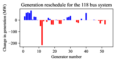
Figure 1: CSCOPF re-dispatch schedule

A contingency analysis was done before and after implementation of the proposed algorithm. Rotor angle trajectories for both cases are shown in Fig. 2. In the figures, the CMs are highlighted in red and orange colors. Without any control, the CMs diverged and eventually lost synchronism. With CSCOPF, these generators remained in sync with the system, effectively alleviating the transient instabilities.

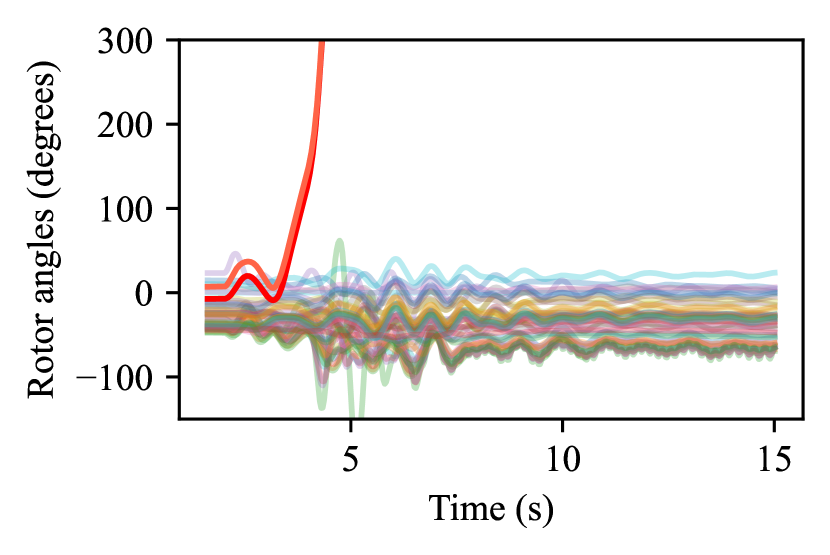
((a)) TDS without CSCOPF

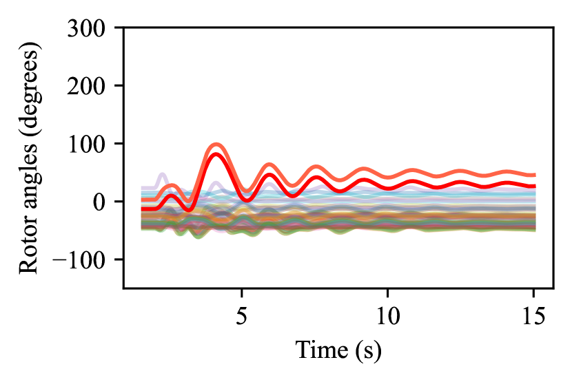
((b)) TDS with CSCOPF

Figure 2: Rotor angle stability for the IEEE 118-bus system.

Table III compares CSCOPF with a conventional real-time security constrained economic dispatch (RT-SCED), and a transient stability constrained OPF (TSCOPF). The RT-SCED does not have cut-set or stability constraints while the TSCOPF solution does not include cut-set constraints and performs SIME in real-time. During implementation, the RT-SCED did not reschedule sufficient generation for ensuring transient stability as it did not have any dynamic information (power from CMs was only lowered by 20 MW as compared to the minimum needed 118 MW shown in Table I). Further, in the identified cut-set, the power flow actually increased instead of decreasing, making that region of the network even more vulnerable to cascading line outages. In comparison, TSCOPF successfully alleviated the transient instabilities, but could not fully address the cut-set overloads (cut-set transfer only reduced by 57 MW as compared to the minimum needed 186 MW shown in Table I). This meant that the system was still at risk of cut-set saturation and line trips.

The proposed CSCOPF alleviated both static and dynamic vulnerabilities resulting in a secure solution without incurring any load shed (see last column of Table III). The solution time of CSCOPF is similar to RT-SCED and one-fourth of TSCOPF, implying that the additional constraints do not significantly increase the computational burden of the optimization, while the data-driven transient stability analyzer actually improves the speed of online operation. From an economic perspective, CSCOPF incurred an additional operational cost of $1728. For context, in absence of any control the simulated wildfire-induced contingency would have put about 534 MW of generation at risk of tripping which would have led to a loss in revenue of at least $12,650, calculated on the generation side. Lastly, although load-shed was not required for the contingency-under-study, it is important to incorporate it in the problem formulation as a different contingency may require both generation re-dispatch as well as load-shed.

TABLE III: Comparative analysis of CSCOPF results

Result	RT-SCED	TSCOPF	CSCOPF
CM generation shed (MW)	20.4	118	269.79
Cut-set desaturation (MW)	-131.80	57.519	187.087
Total load shed (MW)	0	0	0
Transient stable	No	Yes	Yes
Cut-set secure	No	No	Yes
Time to solve (s)	0.066	0.256	0.066
Cost ($/hr)	126,459.97	126,222.28	128,187.95

V Conclusion

In this paper, a comprehensive corrective action scheme addressing both static and dynamic insecurities was introduced that resulted in a resilient power system operation under active wildfire risks. We further proposed a data-driven transient stability constraint prediction model that was able to accurately and reliably predict the appropriate correction factor for mitigating transient instabilities under various loading conditions. The LR-based TSCP algorithm with convex constraints ensured both transparency (in comparison to black-box models) as well as solution optimality. The numerical results indicate that the proposed model is able to detect and alleviate cascading outage risks due to overloaded lines, generators as well as cut-sets, while bearing minimal additional cost. Future work will pivot towards the integration of renewable resources into the CSCOPF problem from both economic as well as stability perspectives.

References

- [1] K. Balaraman, “Wildfires pushed PG&E into bankruptcy. Should other utilities be worried?” Utility Dive, Nov. 19, 2020, https://www.utilitydive.com/news/wildfires-pushed-pge-into-bankruptcy-should-other-utilities-be-worried/588435/.
- [2] D. A. Z. Vazquez, F. Qiu, N. Fan, and K. Sharp, “Wildfire mitigation plans in power systems: A literature review,” IEEE Transactions on Power Systems, vol. 37, no. 5, pp. 3540–3551, 2022.
- [3] M. Choobineh, B. Ansari, and S. Mohagheghi, “Vulnerability assessment of the power grid against progressing wildfires,” Fire Safety Journal, vol. 73, pp. 20–28, 2015.
- [4] NERC, “1,200 MW fault induced solar photovoltaic resource interruption disturbance report: Southern California 8/16/2016 event,” https://www.nerc.com/pa/rrm/ea/Pages/1200-MW-Fault-Induced-Solar-Photovoltaic-Resource-Interruption-Disturbance-Report.aspx.
- [5] S. Dian, P. Cheng, Q. Ye, J. Wu, R. Luo, C. Wang, D. Hui, N. Zhou, D. Zou, Q. Yu, and X. Gong, “Integrating wildfires propagation prediction into early warning of electrical transmission line outages,” IEEE Access, vol. 7, pp. 27 586–27 603, 2019.
- [6] H. Daochun, L. Peng, R. Jiangjun, Z. Yafei, and W. Tian, “Review on discharge mechanism and breakdown characteristics of transmission line gap under forest fire condition,” High Voltage Engineering, vol. 41, no. 2, pp. 622–632, 2015.
- [7] Y. Wu, Y. Xue, J. Lu, Y. XIE, T. XU, W. LI, and C. WU, “Space-time impact of forest fire on power grid fault probability,” Autom Electr Power Syst, vol. 40, no. 3, pp. 14–20, 2016.
- [8] C. Haseltine and L. Roald, “The effect of blocking automatic reclosing on wildfire risk and outage times,” in 2020 52nd North American Power Symposium (NAPS), 2021, pp. 1–6.
- [9] P. Moutis and U. Sriram, “PMU-driven non-preemptive disconnection of overhead lines at the approach or break-out of forest fires,” IEEE Transactions on Power Systems, vol. 38, no. 1, pp. 168–176, 2023.
- [10] J. J. Macwilliams, J. Kobus, and S. L. Monaca, “PG&E: Market and policy perspectives on the first climate change bankruptcy,” 2019.
- [11] R. S. Biswas, A. Pal, T. Werho, and V. Vittal, “A graph theoretic approach to power system vulnerability identification,” IEEE Transactions on Power Systems, vol. 36, no. 2, pp. 923–935, 2020.
- [12] ——, “Mitigation of saturated cut-sets during multiple outages to enhance power system security,” IEEE Transactions on Power Systems, vol. 36, no. 6, pp. 5734–5745, 2021.
- [13] J. Ma, J. C. Cheng, F. Jiang, V. J. Gan, M. Wang, and C. Zhai, “Real-time detection of wildfire risk caused by powerline vegetation faults using advanced machine learning techniques,” Advanced Engineering Informatics, vol. 44, p. 101070, 2020.
- [14] “FlamMap,” US Forest Service, Rocky Mountain Research Station, Fire, Fuel, and Smoke Science Program, https://www.firelab.org/project/flammap, last accessed October 2023.
- [15] M. Abdelmalak and M. Benidris, “Enhancing power system operational resilience against wildfires,” IEEE Transactions on Industry Applications, vol. 58, no. 2, pp. 1611–1621, 2022.
- [16] J. Lu, J. Guo, Z. Jian, and X. Xu, “Optimal allocation of fire extinguishing equipment for a power grid under widespread fire disasters,” IEEE Access, vol. 6, pp. 6382–6389, 2018.
- [17] A. Arab, A. Khodaei, R. Eskandarpour, M. P. Thompson, and Y. Wei, “Three lines of defense for wildfire risk management in electric power grids: A review,” IEEE Access, vol. 9, pp. 61 577–61 593, 2021.
- [18] R. Bayani and S. D. Manshadi, “Resilient expansion planning of electricity grid under prolonged wildfire risk,” IEEE Transactions on Smart Grid, vol. 14, no. 5, pp. 3719–3731, 2023.
- [19] Y. Zhang, L. Wehenkel, and M. Pavella, “SIME: A comprehensive approach to fast transient stability assessment,” IEEJ Transactions on Power and Energy, vol. 118, no. 2, pp. 127–132, 1998.
- [20] A. B. Birchfield, T. Xu, K. M. Gegner, K. S. Shetye, and T. J. Overbye, “Grid structural characteristics as validation criteria for synthetic networks,” IEEE Transactions on Power Systems, vol. 32, no. 4, pp. 3258–3265, 2017.