Comets ¹²CO⁺ and ¹³CO⁺ fluorescence models for measuring the ¹²C/¹³C isotopic ratio in CO⁺

Abstract

Context. CO is an abundant species in comets, creating CO⁺ ion with emission lines that can be observed in the optical spectral range. A good modeling of its fluorescence spectrum is important for a better measurement of the CO⁺ abundance. Such a species, if abundant enough, can also be used to measure the ¹²C/¹³C isotopic ratio.

Aims. This study uses the opportunity of a high CO content observed in the comet C/2016 R2 (PanSTARRS), that created bright CO⁺ emission lines in the optical range, to build and test a new fluorescence model of this species and to measure for the first time the ¹²C/¹³C isotopic ratio in this chemical species with ground-based observations.

Methods. Thanks to laboratory data and theoretical works available in the scientific literature we developed a new fluorescence model both for ¹²CO⁺ and ¹³CO⁺ ions. The ¹³CO⁺ model can be used for coadding faint emission lines and obtain a sufficient signal-to-noise ratio to detect this isotopologue.

Results. Our fluorescence model provides a good modeling of the ¹²CO⁺ emission lines, allowing to publish revised fluorescence efficiencies. Based on similar transition probabilities for ¹²CO⁺ and ¹³CO⁺ we derive a ¹²C/¹³C isotopic ratio of 73$\pm$20 for CO⁺ in comet C/2016 R2. This value is in agreement with the solar system ratio of 89$\pm$2 within the error bars, making the possibility that this comet was an interstellar object unlikely.

1 Introduction

Comets are small icy bodies that remain relatively unaltered by physico-chemical processes since their formation in the outer part of the Solar System. Studying their physical and chemical properties provides useful constraints on the physical and chemical properties of their formation place and, consequently, on the protosolar nebula. These small bodies present some significant differences in their chemical composition but their main species are known for a long time thanks to numerous spectroscopic observations. The main species detected in cometary coma is water molecules with CO and CO₂ being the second most abundant species (typically about 10–20% relative to water).

Carbon monoxide being much more volatile than water this species can drive cometary activity at large distance from the Sun (heliocentric distance larger than 5 au) while water is responsible for the cometary activity usually observed, i.e. for comets closer than about 3 au from the Sun. In the near-UV and optical range, where most of spectroscopic observations are conducted, it is possible to observe CO⁺ emission lines, this ion being created by CO, or indirectly by CO₂. This species has been first reproduced in the laboratory by Fowler (1909a, b) for spectra obtained in the tails of comets C/1907 L2 (Daniel) and C/1908 R1 (Morehouse) and later assigned to CO⁺. The same author later noticed the presence of similar emission bands in Brorsen’s comet observed in 1868 by William Huggins (Fowler, 1910). Swings (1965) mentions observations of CO⁺ bands (now called ”comet tail system of CO⁺”) in the tail of several comets observed after C/1908 R1 (Morehouse).

Emission bands of CO⁺ are, nevertheless, not so often observed in comets. As mentioned above such bands were first observed in the tails of comets at an epoch where spectrographs observed comets at a large scale, covering both the coma and the tail. The instruments later focused on the inner coma, where the signal-to-noise is better and permits to get high-resolution spectra. In this region the detection of CO⁺ species is more difficult. A noticeable exception was the comet C/2016 R2 (PanSTARRS) whose coma presented an unusual composition dominated by the N${}_{2}^{+}$ and CO⁺ ions (Cochran & McKay, 2018; Opitom et al., 2019).

This comet was discovered on September 7, 2016 by the PanSTARRS survey (Weryk & Wainscoat, 2016). It is a long period comet that developed a coma as far as 6 au from the Sun and started to display unusual coma morphology with structure changing rapidly, attributed to ion dominating the emission in the coma. Radio observations revealed a coma dominated by CO with a low abundance of HCN (Wierzchos & Womack, 2018) and optical observations later revealed a spectrum dominated by CO⁺ and N${}_{2}^{+}$ emission bands (Biver et al., 2018; Cochran & McKay, 2018; Opitom et al., 2019). The unusually high abundance of CO⁺ ion in the inner coma of this relatively bright comet (and unusually low abundance of common species like CN and C₂) permitted to get CO⁺ spectra with unprecedented quality (both with high-resolution and high signal-to-noise ratio) for this species with the UVES spectrograph mounted on the 8.2-m ESO VLT telescope, already presented in Opitom et al. (2019).

A correct analysis of such spectra implies a good modeling of the fluorescence spectrum of CO⁺ in comets. Such a modeling has already been done by Magnani & A’Hearn (1986). Nevertheless this work does not present any spectrum that could be confronted to our observational data and some new laboratory and theoretical works have been published after this pioneering work. For these reasons we decided to build a new fluorescence model, based on more recent laboratory data and theoretical works.

In this paper we first present our observational data before explaining in details our model and compare it to the observed spectra. This work also provides new information related to the fluorescence efficiencies. Because such data also open the possibility, for the first time, to measure the ¹²C/¹³C isotopic ratio in CO⁺ we also computed a fluorescence model of the ¹³CO⁺ isotopologue and searched for its emission lines. The result of the search of these faint lines is also presented, leading to a first estimate of the ¹²CO⁺/¹³CO⁺ ratio in a comet.

2 Observational data

The spectra used for this work have been obtained with the Ultraviolet-Visual Echelle Spectrograph (UVES) mounted on the ESO 8.2 m UT2 telescope of the Very Large Telescope (VLT) located in Chile. They correspond to the dichroic #1 (390+580 settings) covering the range 326 to 454 nm in the blue and 476 to 684 nm in the red and the dichroic #2 (437+860 settings) covering the range 373 to 499 nm in the blue and 660 to 1060 nm in the red (the data obtained in this last spectral range have not been used for this work). Three different observing nights have been used for observations with the dichroic #1, corresponding to February 11, 13 and 14, 2018. During each night one single exposure of 4800 s of integration time was obtained. We used a 0.44” wide slit, providing a resolving power of R$\sim$80,000. The slit length was 8” for the setting 390 corresponding to about 14,500 km at the distance of the comet (geocentric distance of 2.4 au) and 12” for the setting 580. The average heliocentric distance was 2.76 au and the heliocentric velocity 5.99 km s^-1. The observations performed with dichroic #2 (437+860) correspond to two observing nights on February 15 and 16. In that case a single exposure of 3000 s of integration time was obtained for both nights and the slit width was also 0.44” with a slit length of 10” (for the setting 437). Opitom et al. (2019) provides more details about these observations.

As explained by these authors the data were reduced using the ESO UVES pipeline, combined with custom routines to perform the extraction, cosmic rays removal, and then corrected for the Doppler shift due to the relative velocity of the comet with respect to the Earth. The spectra are calibrated in absolute flux using either the archived master response curve or the response curve determined from a standard star observed close to the science spectrum (with no significant differences between these two methods). This data processing produced 2D spectra calibrated in wavelength and absolute flux units. Because a close examination of the ESO UVES sky emission spectrum permits to check that telluric lines are below the noise level in this part of the spectrum no specific data processing was done for removing these lines.

From these three different settings (390, 580 and 437) we computed average 1D spectra. These 1D spectra were further splitted in different parts corresponding to the different CO⁺ emission bands. The solar continuum has been subtracted for each of these different spectra individually in order to adjust it as well as possible in a limited spectral range. Many CO⁺ bands can be identified in our observational data (see section 5 for more details).

3 ¹²CO⁺ fluorescence model

The CO⁺ emission lines observed in the optical range belong to the comet tail system, i.e. to the A${}^{2}\Pi_{i}$–X${}^{2}\Sigma^{+}$ electronic transition. The A${}^{2}\Pi_{i}$ state is divided into two branches (${}^{2}\Pi_{1/2}$ and ${}^{2}\Pi_{3/2}$ labeled $F_{2}$ and $F_{1}$) with a large energy separation because the $2\Pi$ electronic state is intermediate between Hund’s case (a) and (b) (the $F_{2}$ states corresponding to higher energies). The rotational levels are split as a result of $\Lambda$-doubling. Such a rotational structure gives rise to 12 branches and each band is divided into two sub-bands corresponding to the ${}^{2}\Pi_{1/2}$–$X^{2}\Sigma^{+}$ and ${}^{2}\Pi_{3/2}$–$X^{2}\Sigma^{+}$ transitions. Fig. 1 presents the energy levels diagram with the different types of lines involved in this transition.

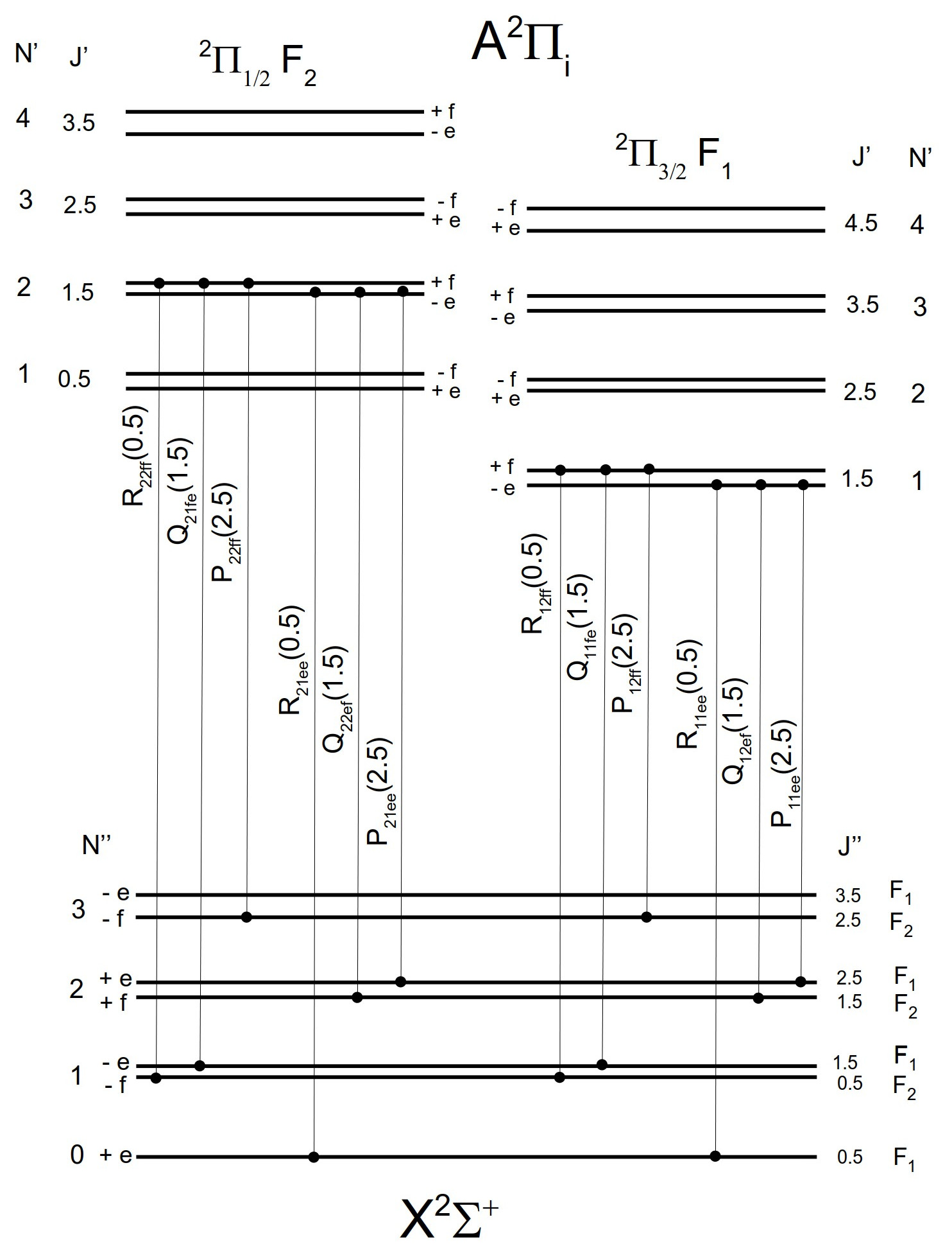
Figure 1: Energy level diagram showing the A${}^{2}\Pi_{i}$–X${}^{2}\Sigma^{+}$ transition with the different lines involved by this transition. The number in parenthesis refers to the $J^{\prime\prime}$ value of the line.

A pioneering work was published by Magnani & A’Hearn (1986) that presents a fluorescence model for CO⁺ in cometary coma. This paper does not show any comparison between synthetic spectra and observational data. For modeling the ¹²CO⁺ and ¹³CO⁺ in comet C/2016 R2 it appears necessary to develop a new fluorescence model that can benefit from different experimental and theoretical articles published after Magnani & A’Hearn’s paper. Such works can significantly help to improve this modeling. Magnani & A’Hearn (1986) contains nevertheless interesting data to built such a new fluorescence model.

We developed our own fluorescence model of CO⁺ that takes into account the A${}^{2}\Pi_{i}$ and X${}^{2}\Sigma^{+}$ electronic levels with the first 6 vibronic levels ($v=0$ to $5$). The energy levels for the X${}^{2}\Sigma^{+}$ state and the first three vibrational quantum numbers $v$ equal to 0, 1 and 2 have been taken from Hakalla et al. (2019), as well as the $v=0,1$ vibronic energy levels of the A${}^{2}\Pi_{i}$ state. From the X${}^{2}\Sigma^{+}$ $v=0$ levels accurate energy levels of the A${}^{2}\Pi_{i}$ $v=2,3,4$ states have been computed with the transition frequencies published by Kepa et al. (2004) for the (2,0), (3,0) and (4,0) bands. The remaining energy levels ($v=3,4,5$ of the X${}^{2}\Sigma^{+}$ state and $v=5$ of the A${}^{2}\Pi_{i}$ state) have been computed from the molecular parameters published by Kepa et al. (2004) (rotational constants) and Coxon et al. (2010) (band origin). All the levels with a rotational quantum number $J\leq 10.5$ have been taken into account in our model.

The Einstein coefficients for the spontaneous transition probabilities have been computed with the transition probabilities computed by Billoux et al. (2014) expressed in atomic units. These values need to be converted to spontaneous emission Einstein coefficients $A_{ul}$ from the upper level $u$ to the lower level $l$ of a given line by using the following formula (case of a $\Pi$–$\Sigma$ transition):

$$A_{ul}=2.026\times 10^{-6}\times\sigma_{ul}^{3}\times p^{v^{\prime}v^{\prime\prime}}_{N^{\prime}N^{\prime\prime}}{S_{J^{\prime}J^{\prime\prime}}\over 2J^{\prime}+1}$$

with $p^{v^{\prime}v^{\prime\prime}}_{N^{\prime}N^{\prime\prime}}$ being the transition probability provided by Billoux et al. (2014) expressed in atomic units, $\sigma_{ul}$ the wavenumber expressed in cm^-1, $J^{\prime}$ the rotational quantum number of the upper state and $S_{J^{\prime}J^{\prime\prime}}$ the Hönl-London factor.

The Hönl-London factors have been taken from Arpigny (1964b) and renormalized to follow the summation rule used by Billoux et al. (2014), i.e.:

$$\sum_{J^{\prime}}S_{J^{\prime}J^{\prime\prime}}=(2-\delta_{0,\Lambda^{\prime}+\Lambda^{\prime\prime}})(2S^{\prime}+1)(2J^{\prime\prime}+1)$$

The Einstein absorption coefficients $B_{lu}$ have been computed from the $A_{ul}$ coefficients and the wavenumbers of the corresponding transitions. The probability of absorption is given by $B_{lu}\times\rho_{\nu}$ with $\rho_{\nu}$ being the radiation density at the corresponding wavelength, expressed in erg.cm^-3.Hz^-1. We used the high-resolution solar spectrum published by Kurucz et al. (1984) to compute the solar radiation density.

The pure vibrational transition probabilities of the ground X${}^{2}\Sigma^{+}$ state have been taken in Rosmus & Werner (1982) (A${}_{v^{\prime}v^{\prime\prime}}$ Einstein coefficients) with Hönl-London factors from Magnani & A’Hearn (1986). The pure rotational transition probabilities have been computed from the formulae published by Arpigny (1964a) for a ${}^{2}\Sigma$ state in using an electric dipole moment $\mu=2.771$ Debye (Bell et al., 2007).

Apart the ground electronic state $X^{2}\Sigma^{+}$ and the first electronic excited state $A^{2}\Pi_{i}$ there is another excited electronic state $B^{2}\Sigma^{+}$ with a $B^{2}\Sigma^{+}$–$X^{2}\Sigma^{+}$ transition called first negative system and a $B^{2}\Sigma^{+}$–$A^{2}\Pi_{i}$ transition called Baldet-Johnson system (see Fig. 1 in Magnani & A’Hearn (1986)). Because the first negative system B${}^{2}\Sigma^{+}$–X${}^{2}\Sigma^{+}$ transition can also slightly influence the relative populations of the ground electronic state some levels in the B${}^{2}\Sigma^{+}$ ($v=0,1,2$) have also being taken into account in our modeling with the first negative system (the Baldet-Johnson system implying two excited electronic states its influence can be neglected). The energy levels of the $B^{2}\Sigma^{+}$ have been computed with the molecular parameters published by Szajna et al. (2004) and the transition probabilities are taken from Magnani & A’Hearn (1986).

The relative population have been computed at the equilibrium with the method described by Zucconi & Festou (1985). Such a method is justified by the heteronuclear nature of the CO⁺ ion that involves pure vibrational and rotational transitions that permit to reach the fluorescence equilibrium with a timescale well below the time spent by these ions in the observed cometary coma (this is not the case for homonuclear species like, e.g. C₂ or N${}_{2}^{+}$). We assume that the coma is an optically thin medium for this spectrum, i.e. that the radiation received by the telescope is proportional to the number of CO⁺ ions along the line of sight with the radiation emitted in units of energy in $4\pi$ steradian equal to $x_{i}\times h\nu$, $x_{i}$ being the relative population, $h$ the Planck’s constant and $\nu$ the frequency.

4 ¹³CO⁺ fluorescence model

For this isotopologue the energy levels comes from the laboratory data published by Kepa et al. (2002): we used the (1,0), (3,0), (4,0) and (5,0) bands wavenumbers of the lines observed to reconstruct all the energy levels of the X${}^{2}\Sigma^{+}$ state $v=0$. From this state it was then possible to compute the energy levels of the A${}^{2}\Pi_{i}$ $v=1,2,3,4,5$ states by using the (1,0)(2,0)(3,0)(4,0)(5,0) transitions. After this computation the X${}^{2}\Sigma^{+}$ state $v=1$ was computed by using the (2,1) band wavenumbers. Such a method provide a high accuracy for the final wavelength (accuracy of about 0.01 Å, well below the FWHM of our high-resolution spectra). The missing energy levels were computed from the molecular parameters published by Kepa et al. (2002) for the A${}^{2}\Pi_{i}$ $v=0$ state and X${}^{2}\Sigma^{+}$ state $v=2,3,4,5$.

For the B${}^{2}\Sigma^{+}$ level we also used the molecular constants published by Szajna et al. (2004) but adapted for the ¹³CO⁺ isotopologue. It was done by using the reduced atomic mass $\mu^{\prime}$ of this isotopologue and the one of ¹²CO⁺ ($\mu$) providing the parameter $\rho=\sqrt{\mu/\mu^{\prime}}=0.9777$. This parameter was used to compute the molecular parameters of ¹³CO⁺ from the ones of ¹²CO⁺ thanks to the formulae given by Herzberg, G. (1950).

The transition probabilities have been assumed to be equal to the ones of ¹²CO⁺, such an approximation is justified by some calculations done for other diatomic species that show only small relative differences for the transition probabilities for different isotopologues (see, e.g., Ferchichi et al. (2022) for the different isotopologues of N${}_{2}^{+}$).

5 Comparison with observational data and fluorescence efficiencies

The ¹²CO⁺ emission lines being clearly visible in our C/2016 R2 spectra it is possible to check, for the first time, with a high accuracy the quality of our fluorescence model developed for this isotopologue. Our observational data permit to observe different bands with the three different UVES settings mentioned in section 2. These settings corresponding to different slit sizes, epochs of observations or exposure times they show different relative intensities of the spectra.

We computed the ¹²CO⁺ fluorescence spectrum for the condition of observations of C/2016 R2 and adjusted its intensity for each setting. We kept the same relative intensity for all the different bands observed with a same setting, in order to check the accuracy of the relative intensities provided by our model for different bands. Fig. 2 provides an overview of all the CO⁺ emission bands identified in our observations, for the three different settings used for this work.

For a better comparison between observational data and the synthetic spectrum Fig. 3, Fig. 4 and Fig. 5 zooms on different bright bands to show the details of the rotational structure. The relative intensities for the different bands agree well with the observational data.

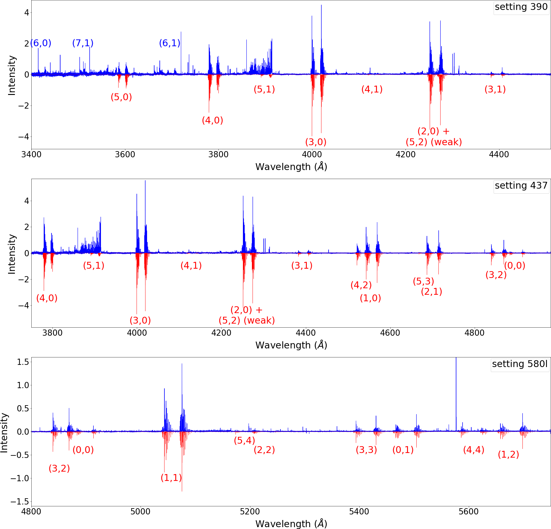
Figure 2: Comparison of our modeling of ¹²CO⁺ spectrum with our observational data obtained on comet C/2016 R2 for the three different settings. The observational spectra appear in blue while the model is in red (for more clarity it appears with a negative scale). The different CO⁺ bands bright enough to be detected in the observational spectrum are identified in red for the model. The (6,0), (7,1) and (6,1) CO⁺ bands appear (weakly) on the observational spectrum and are identified in blue, but not on the model because this one is restricted to $v^{\prime\prime}$ and $v^{\prime}\leq 5$. The intensity scale is arbitrary but proportional to units of ergs.s^-1. Some other species appear in the observational spectrum (e.g. N${}_{2}^{+}$ and CN emission lines near the (5,1) CO⁺ band).

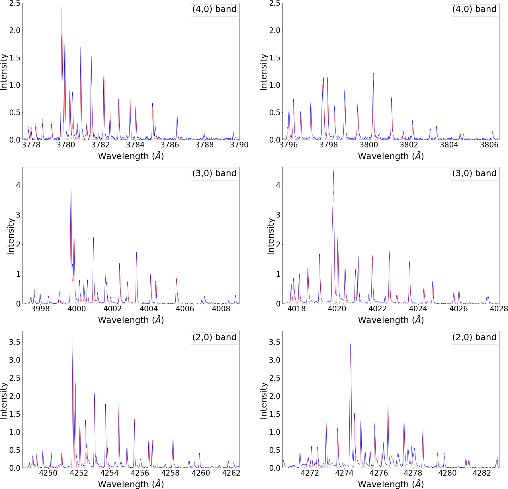
Figure 3: Comparison of our modeling of ¹²CO⁺ spectrum with our observational data obtained on comet C/2016 R2, for different bands observed with the setting 390. The intensity scale is arbitrary but proportional to units of ergs.s^-1 and is the same for the different bands. The observational spectrum appears in blue while the modeling is in red. The emission lines of the (2,0) band are blended with some emission lines of the (5,2) band but this band represents only a few percent in intensity with respect to the (2,0) band.

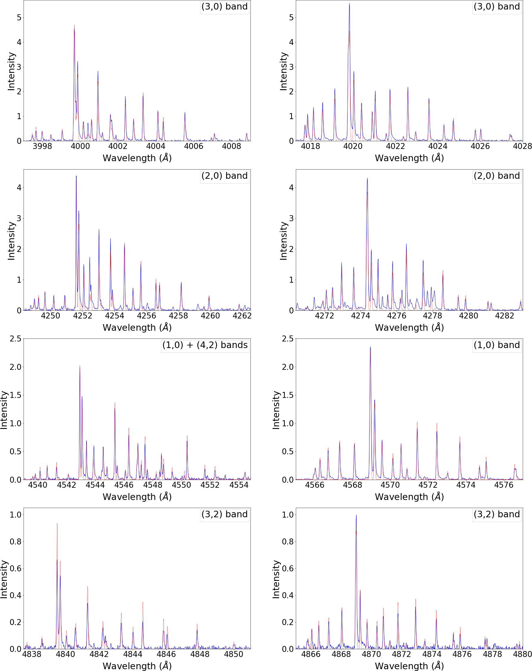
Figure 4: Comparison of our modeling of ¹²CO⁺ spectrum with our observational data obtained on comet C/2016 R2, for different bands observed with the setting 437. The intensity scale is arbitrary but proportional to units of ergs.s^-1 and is the same for the different bands. The observational spectrum appears in blue while the modeling is in red. The emission lines of (1,0) $\Pi_{1/2}$ band are mixed with the emission lines of the (4,2) $\Pi_{3/2}$ band, these last ones being fainter (intensities roughly equal to the ones of the (3,2) $\Pi_{3/2}$ band).

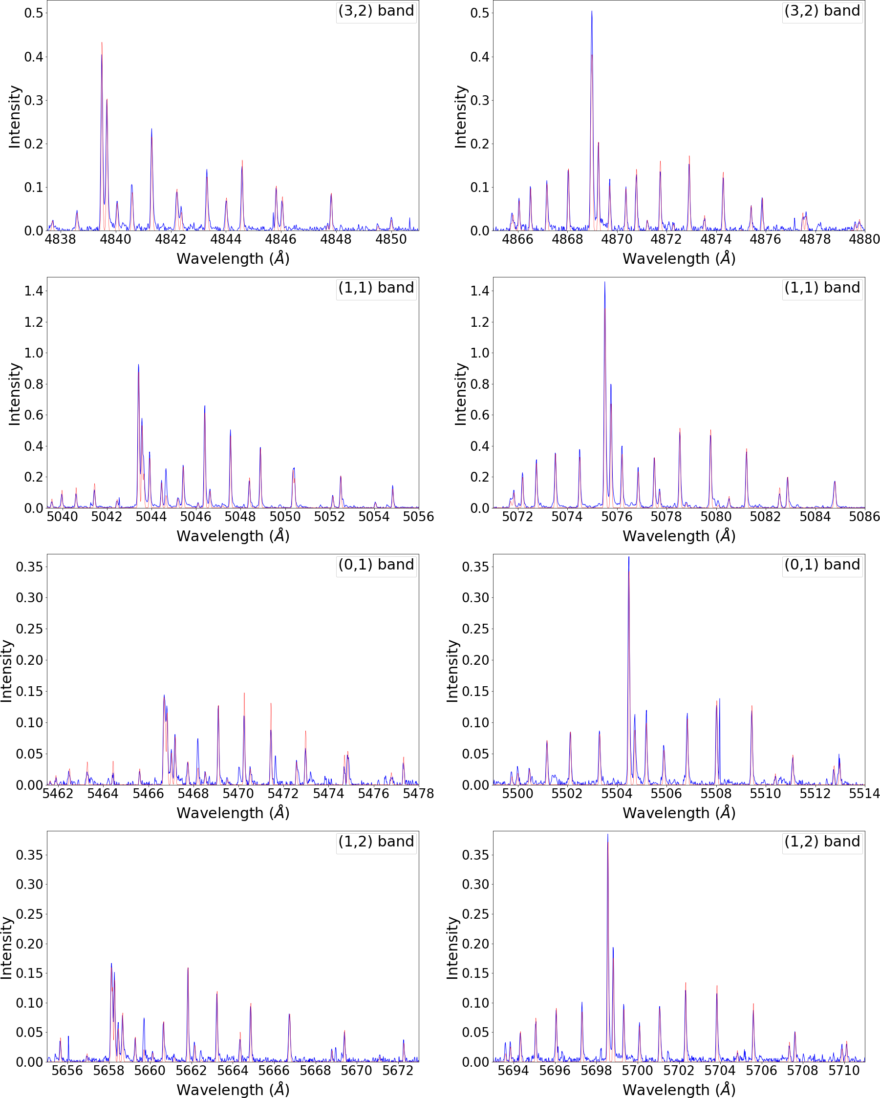
Figure 5: Comparison of our modeling of ¹²CO⁺ spectrum with our observational data obtained on comet C/2016 R2, for different bands observed with the setting 580l. The intensity scale is arbitrary but proportional to units of ergs.s^-1 and is the same for the different bands. The observational spectrum appears in blue while the modeling is in red.

We can compute fluorescence efficiencies, also called $g$-factors or band luminosities with our fluorescence model. Table 1 provides an overview of these important parameters for an heliocentric distance of 1 au and an heliocentric velocity of 0 km.s^-1. A comparison of this parameter with the results published by Magnani & A’Hearn (1986) in their Table 3 permits to see a similar value for the (4,0) band ($1.07\times 10^{-14}$ vs $1.04\times 10^{-14}$ erg.s^-1.ion${}^{-}1$), which is one of the brightest band. The relative differences in intensities between our model and the results published by Magnani & A’Hearn (1986) can reach a factor of about two for some bands. For the brightest ones (i.e. (3,0), (2,0) and (4,0) by decreasing intensity), that are displayed Fig. 3 (and Fig. 4 for (2,0) and (3,0)) our modeling shows a good fit with the observational data. Our computed intensity ratio $g(3,0)/g(4,0)=1.63$ appears in good agreement with the observational data but disagrees with the ratio computed by Magnani & A’Hearn (1986), which is $2.03$ and that would not be able to fit such observational data as well as our model. We have no possibility to test the absolute values of the band luminosities but our fit of the different bands confirms that their relative values are robust, at least to about 10%. Fig. 6 shows the variation of fluorescence efficiencies as a function of the heliocentric velocity for the four brightest bands (i.e. (3,0), (2,0), (4,0) and (1,1) by decreasing intensity). Some variations can be observed but they remain limited to less than about 15% between the smaller and the larger values. We also computed the product of the fluorescence efficiency by the square of heliocentric distance $R_{h}$ (expressed in au) in order to check if there is any significant deviation from the usual scaling law with this parameter. Only some small variations can be observed (see Table 2).

Table 1: Fluorescence efficiencies computed for ¹²CO⁺, for the heliocentric distance $r_{h}=1$ au and the heliocentric velocity $v_{h}=0$ km.s^-1, in units of erg.s^-1.ion^-1.

	$v"=0$	1	2	3	4	5
$v^{\prime}$
0	8.40$\times 10^{-16}$	1.87$\times 10^{-15}$	1.81$\times 10^{-15}$	9.99$\times 10^{-16}$	3.45$\times 10^{-16}$	7.63$\times 10^{-17}$
1	7.68$\times 10^{-15}$	8.41$\times 10^{-15}$	2.19$\times 10^{-15}$	7.10$\times 10^{-18}$	7.63$\times 10^{-16}$	7.87$\times 10^{-16}$
2	1.36$\times 10^{-14}$	5.38$\times 10^{-15}$	9.28$\times 10^{-17}$	2.25$\times 10^{-15}$	1.03$\times 10^{-15}$	2.94$\times 10^{-18}$
3	1.70$\times 10^{-14}$	9.24$\times 10^{-16}$	3.07$\times 10^{-15}$	1.90$\times 10^{-15}$	5.49$\times 10^{-17}$	8.79$\times 10^{-16}$
4	1.04$\times 10^{-14}$	1.97$\times 10^{-16}$	2.96$\times 10^{-15}$	2.23$\times 10^{-17}$	9.53$\times 10^{-16}$	2.80$\times 10^{-16}$
5	5.12$\times 10^{-15}$	1.21$\times 10^{-15}$	1.04$\times 10^{-15}$	4.14$\times 10^{-16}$	5.21$\times 10^{-16}$	4.16$\times 10^{-17}$

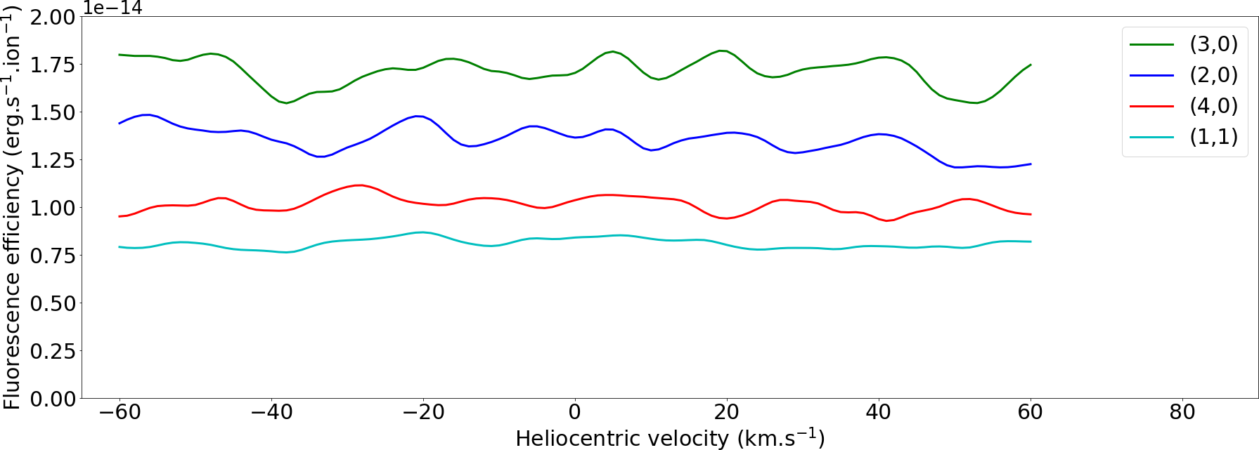
Figure 6: Fluorescence efficiencies of the four brightest CO⁺ bands as a function of the heliocentric velocity.

Table 2: Fluorescence efficiencies multiplied by $R_{h}^{2}$ computed for ¹²CO⁺.

	$R_{h}=0.5$ au	$1.0$	$1.5$	$2.0$	$3.0$	$4.0$
band
(2,0)	1.35$\times 10^{-14}$	1.36$\times 10^{-14}$	1.37$\times 10^{-14}$	1.38$\times 10^{-14}$	1.39$\times 10^{-14}$	1.41$\times 10^{-14}$
(3,0)	1.67$\times 10^{-14}$	1.70$\times 10^{-14}$	1.72$\times 10^{-14}$	1.74$\times 10^{-14}$	1.77$\times 10^{-14}$	1.79$\times 10^{-14}$
(4,0)	1.02$\times 10^{-14}$	1.04$\times 10^{-14}$	1.04$\times 10^{-14}$	1.03$\times 10^{-14}$	1.01$\times 10^{-14}$	9.94$\times 10^{-15}$
(1,1)	8.28$\times 10^{-15}$	8.41$\times 10^{-15}$	8.46$\times 10^{-15}$	8.47$\times 10^{-15}$	8.47$\times 10^{-15}$	8.43$\times 10^{-15}$

We also computed fluorescence efficiencies for ¹³CO⁺ (see Table 3). As we assumed that ¹³CO⁺ and ¹²CO⁺ have similar transition probabilities these band luminosities are very close to the ones of ¹²CO⁺ but some differences appear due to the wavelength shifts that implies some variations in the solar flux for absorption transitions. Such fluorescence efficiencies can be useful for future ¹²C/¹³C isotopic ratio measurements in CO⁺ (see below).

Table 3: Fluorescence efficiencies computed for ¹³CO⁺, for the heliocentric distance $r_{h}=1$ au and the heliocentric velocity $v_{h}=0$ km.s^-1, in units of erg.s^-1.ion^-1.

	$v"=0$	1	2	3	4	5
$v^{\prime}$
0	8.89$\times 10^{-16}$	1.99$\times 10^{-15}$	1.96$\times 10^{-15}$	1.10$\times 10^{-15}$	3.88$\times 10^{-16}$	8.85$\times 10^{-17}$
1	6.84$\times 10^{-15}$	7.56$\times 10^{-15}$	1.99$\times 10^{-15}$	6.55$\times 10^{-18}$	7.16$\times 10^{-16}$	7.55$\times 10^{-16}$
2	1.38$\times 10^{-14}$	5.49$\times 10^{-15}$	9.56$\times 10^{-17}$	2.34$\times 10^{-15}$	1.09$\times 10^{-15}$	3.17$\times 10^{-18}$
3	1.65$\times 10^{-14}$	9.03$\times 10^{-16}$	3.02$\times 10^{-15}$	1.89$\times 10^{-15}$	5.53$\times 10^{-17}$	8.98$\times 10^{-16}$
4	7.69$\times 10^{-15}$	1.47$\times 10^{-16}$	2.23$\times 10^{-15}$	1.68$\times 10^{-17}$	7.29$\times 10^{-16}$	2.17$\times 10^{-16}$
5	5.40$\times 10^{-15}$	1.28$\times 10^{-15}$	1.11$\times 10^{-15}$	4.46$\times 10^{-16}$	5.66$\times 10^{-16}$	4.57$\times 10^{-17}$

6 Measurement of ¹²CO⁺/¹³CO⁺ isotopic ratio in comet C/2016 R2

The high signal-to-noise and spectral resolution of our observational data opens the possibility, for the first time, to measure the ¹²C/¹³C isotopic ratio in the CO⁺ species with ground-based observations. It is possible thanks to the wavelength shift between the spectrum of the two isotopologues. Fig. 7 presents the synthetic spectra of these two isotopologues superimposed to the observational data of the brightest band (i.e. the (3,0)). It can be seen that the ¹³CO⁺ emission lines are clearly separated of the ¹²CO⁺ ones. At this intensity scale no ¹³CO⁺ emission lines are visible.

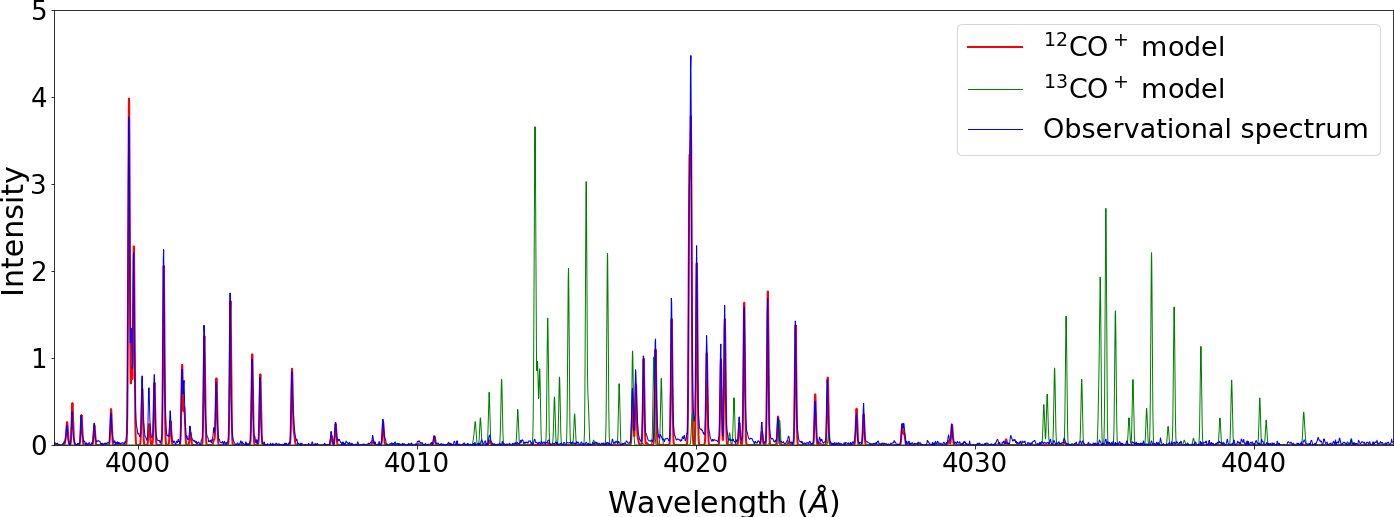
Figure 7: ¹²CO⁺ and ¹³CO⁺ theoretical spectra superimposed to the observational data obtained on comet C/2016 R2. The relative intensity of ¹³CO⁺ emission lines are based on the ¹²CO⁺ fit of the emission lines. They do not respect the intensities observed in this comet, the purpose of this plot being only to show the wavelength shift between the emission lines of these two isotopologues.

To increase the signal-to-noise ratio of the possible ¹³CO⁺ emission lines we decided to coadd the brightest ¹³CO⁺ emission lines for the two brightest bands, i.e. the (3,0) and (2,0). The wavelengths have been carefully chosen to avoid any other possible emission lines due to other species. At the end we restricted our choice to 15 lines belonging to the (3,0) band and 9 lines for the (2,0) band. Their counterpart for the ¹²CO⁺ were also coadded. Table 4 provides the details of the lines wavelengths used as well as their ¹²CO⁺ counterparts. The work here was facilitated because C/2016 R2 is very poor in the usual bright and abundant lines of CN and C₂ in the CO⁺ regions of interest.

Table 4: Wavelengths (Å) of the ¹³CO⁺ lines coadded to measure the ¹²C/¹³C isotopic ratio with their ¹²CO⁺ counterpart.

Band	13CO+	12CO+ counterpart
(3,0)	4032.600	4017.855
(3,0)	4032.865	4018.135
(3,0)	4033.275	4018.560
(3,0)	4033.835	4019.140
(3,0)	4034.500	4019.825
(3,0)	4034.700	4020.040
(3,0)	4035.045	4020.395
(3,0)	4035.670	4021.045
(3,0)	4036.340	4021.740
(3,0)	4036.930	4022.375
(3,0)	4038.790	4024.285
(3,0)	4039.210	4024.730
(3,0)	4040.215	4025.765
(3,0)	4040.445	4026.020
(3,0)	4041.790	4027.402
(2,0)	4283.360	4272.445
(2,0)	4283.840	4272.950
(2,0)	4284.480	4273.620
(2,0)	4285.200	4274.370
(2,0)	4285.425	4274.600
(2,0)	4285.780	4274.970
(2,0)	4286.295	4275.510
(2,0)	4288.195	4277.475
(2,0)	4290.445	4279.825

Thanks to the coaddition of these lines we managed to detect a ¹³CO⁺ coadded emission line well above the background noise. The coaddition of the ¹²CO⁺ emission lines counterpart and their fit with our fluorescence model allowed us to derive the ¹²C/¹³C isotopic ratio in the CO⁺ by adjusting our ¹³CO⁺ fluorescence model (coaddition of the same lines) to the observational data (see Fig. 8). This method provided ¹²C/¹³C=$73\pm 20$. The main source of uncertainty comes from the exact backround level that needs to be adjusted with a high accuracy. A good test for the adjustement of this level, apart that the intensities should be positive and a background close to zero in between the emission lines, is the quality of the fit with our modeling. The quality of this fit is very good for the FWHM if the model is adjusted to observational data with background close to zero. If it is not the case, some discrepancies in the line width appear.

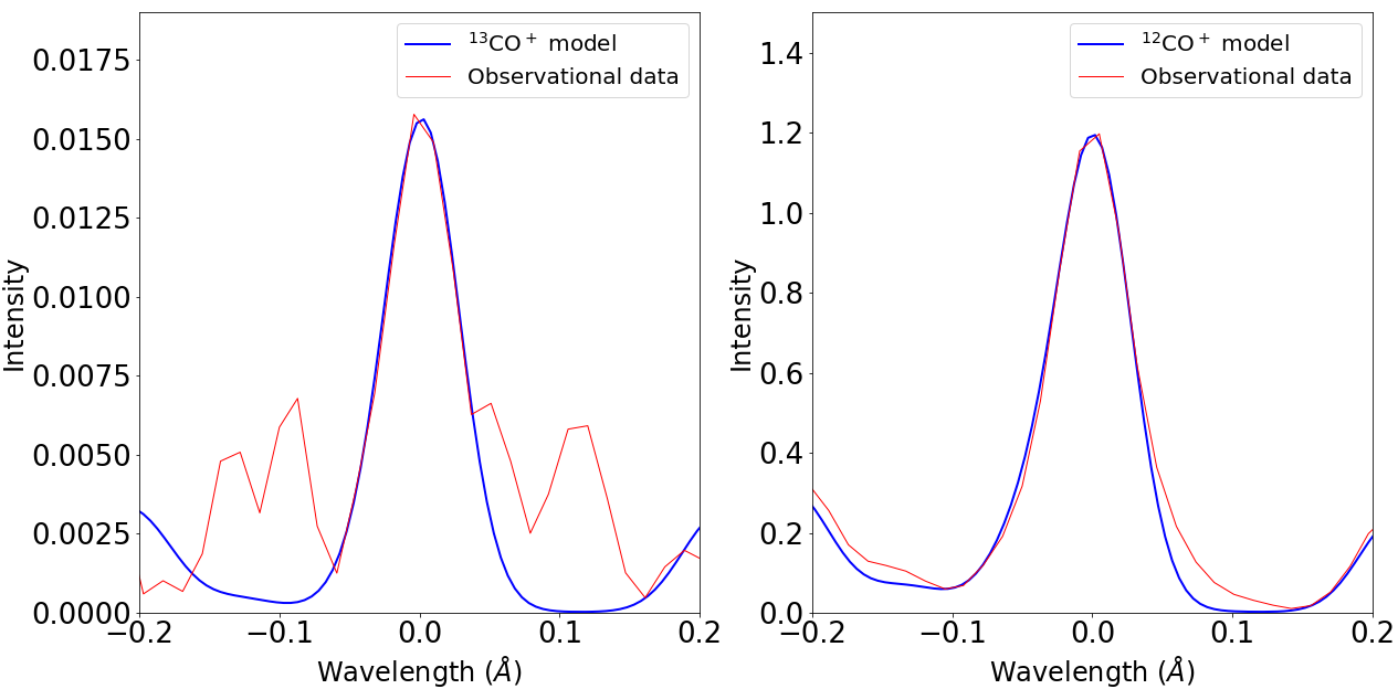
Figure 8: Coaddition of the brightest (3,0) and (2,0) emission lines of ¹³CO⁺ (left) and ¹²CO⁺ (right) with the corresponding modeling (see Table 4 for the detailed list of coadded lines).

This estimate of the ¹²C/¹³C isotopic ratio in CO⁺ is similar to the other measurements done in the optical in C₂ and CN (Manfroid et al., 2009), and in the submm region for HCN. This ratio has been measured so far from ground-based facilities in dozens of comets (Bockelée-Morvan et al., 2015). Some other in situ measurements were more recently performed in the coma of comet 67P/Churyumov-Gerasimenko by the ROSINA mass spectrometer on-board the Rosetta spacecraft for C₂H₄, C₂H₅, CO (Rubin et al., 2017) and CO₂ (Hässig et al., 2017) molecules. These measurements varies from about 60 (measured in C₂ for comet West 1976 IV, Lambert & Danks (1983)) to 165 (measured in CN with comet C/1995 O1 (Hale-Bopp) by Arpigny et al. (2003)) with large errorbars. Most of them are compatible with the terrestrial value of 89, within their (often large) errorbars. For CO in comet 67P, the ¹²C/¹³C ratio measured is 86$\pm$9 (Rubin et al., 2017), i.e. is compatible with our result within the errorbars. This one is the first ever published for the CO⁺ species.

7 Conclusion

Thanks to high quality observational data obtained on comet C/2016 R2, a comet exceptionally rich in both CO⁺ and N${}_{2}^{+}$ in the inner coma, it was possible to test in detail a new fluorescence model of ¹²CO⁺, that takes into account new laboratory data and theoretical works obtained since the pioneering work of Magnani & A’Hearn (1986). The confrontation of this model with our spectra provides good results, confirming the efficiency of this model. Some new fluorescence efficiencies (g-factors) are also published, which are in relatively good agreement with observational data for the relative intensities. Such revised g-factors can be used in the future for more accurate measurement of CO⁺ abundance in comets. Previous estimate of such abundances can now also be slightly revised. For example the N₂/CO ratio computed by Opitom et al. (2019) and based on the g-factor of the (2,0) band published by Magnani & A’Hearn (1986) can be revised (in addition to the revised g-factors published for N${}_{2}^{+}$ by Rousselot et al. (2022) and used by Anderson et al. (2022)). The new ratio CO⁺/N${}_{2}^{+}$ should be reduced by about 20% according to our revised values.

Our ¹³CO⁺ fluorescence model also opens the possibility of new measurements of the ¹²C/¹³C isotopic ratio in the CO⁺ species. This work shows that such a measurement becomes possible and provided a value of 73$\pm$20 for comet C/2016 R2, in agreement with other similar measurements conducted in other species and in the in situ measurement obtained in the coma of comet 67P by ROSINA mass spectrometer. This value probably excludes that the very peculiar comet C/2016 R2 would be of interstellar origin.