Measuring the nuclear equation of state with neutron star-black hole mergers

Abstract

Gravitational-wave (GW) observations of neutron star-black hole (NSBH) mergers are sensitive to the nuclear equation of state (EOS). Using realistic simulations of NSBH mergers, incorporating both GW and electromagnetic (EM) selection to ensure sample purity, we find that a GW detector network operating at O5-sensitivities will constrain the radius of a $1.4\,\mathrm{M_{\odot}}$ NS and the maximum NS mass with $1.6\%$ and $13\%$ precision, respectively. The results demonstrate strong potential for insights into the nuclear EOS, provided NSBH systems are robustly identified.

Introduction. A key aim of modern physics is to understand the behavior of nuclear matter at high densities, and in particular the nuclear equation of state (EOS). However, constraints above the nuclear saturation density are currently beyond the realm of terrestrial experiments [e.g., 1, 2]. For the moment, such progress can only come from observations of extreme astrophysical systems, such as neutron stars (NSs) [e.g., 3, 4].

There are several distinct astronomical probes of NS physics, including electromagnetic (EM) observations in the radio [e.g., 5, 6] and X-rays, such as those being made by the Neutron Star Interior Composition Explorer (NICER) mission [e.g., 7], as well as gravitational wave (GW) observations. The latter possibility was first demonstrated by the multi-messenger GW and EM observations of the binary neutron star (BNS) merger GW170817, which directly measured the NS tidal deformability [8, 9, 10, 11]. These constraints will improve as more BNS mergers are identified and characterized, although the expected rate of new discoveries is highly uncertain [12].

The GW emissions produced by neutron star-black hole (NSBH) mergers are also sensitive to the NS tidal deformability [13, 14], providing a distinct way of measuring both the high-density nuclear EOS and the BH and NS mass and spin distributions [15]. Importantly, NSBH systems have higher total masses than BNSs and so produce stronger GW signals that are detectable at considerably greater distances. And, while the rate of NSBH mergers is also highly uncertain [12], it is possible that they could come to dominate over BNS mergers in terms of detected numbers. If so, NSBH mergers could potentially provide the best constraints on the high-density nuclear EOS, a possibility we explore here.

We begin by describing our simulations, including the combined EM and GW selection of multi-messenger events. We then outline the analysis framework used to infer the BH and NS mass distributions and the nuclear EOS from the simulated samples. We present a new methodology which is also able to provide constraints on the magnitude, length scale, and location in energy density of structure in the EOS. We conclude by discussing improvements in the analysis chain that would be required in order to obtain reliable constraints from real multi-messenger observations of NSBH mergers.

Simulations. We start by defining a population model of NSBH systems motivated both by stellar population synthesis simulations [16] and current astrophysical constraints [12]. We assume a constant (non-evolving) NSBH merger rate of $\Gamma=32$ ${\rm yr^{-1}\,Gpc^{-3}}$, corresponding to the median from population analyses of the third LVK GW catalog [12]. The NSBH mergers are distributed uniformly in comoving volume and isotropically over the sky. We assume truncated normal mass distributions: $P(m_{\rm BH}/M_{\odot})=\mathcal{N}(\mu=15,\sigma=10,a=2.42,b=55)$; and $P(m_{\rm NS}/M_{\odot})=\mathcal{N}(\mu=1.5,\sigma=0.3,a=1.1,b=2.1)$. We adopt the DD2 EOS [17] and use the maximum implied NS mass as the lower limit for the BH mass distribution. However, we restrict the NS mass distribution to be truncated at a lower mass as these quantities likely differ due to NSBH formation processes [e.g., 18]. For the distribution of BH and NS spins, which we assume to be aligned, we adopt $P(\chi_{\rm BH})=\rm{Beta}(\alpha=0.1,\beta=0.5)$ and $P(a_{\rm NS})=\rm{Uniform}(0,0.05)$, respectively. We set the BH tidal deformability to $\Lambda_{\rm BH}=0$; $\Lambda_{\rm NS}$ is set by the component masses and the DD2 EOS.

We simulate observations for a $5$-detector GW network at O5-sensitivities, expected to operate from 2027 [19]. This network consists of two LIGO A+ [20], Advanced Virgo [21], KAGRA [22], and LIGO India [23, 19], for which sensitivity curves are available . We assume an observing time of $t_{\rm obs}=5\,\mathrm{yrs}$ with a duty cycle of $\Delta_{\rm obs}=0.5$.

We begin by drawing the total number of mergers from a Poisson distribution with mean $\lambda=4\pi/3\,\Delta_{\rm obs}\,t_{\rm obs}\,D_{L,\rm{max}}^{3}\,\Gamma$, where $D_{L,\rm{max}}{}=3,500\,\mathrm{Mpc}$ is the highest luminosity distance at which the most massive NSBH merger could be detected in O5 for our population, consistent with horizon distance measurements of NSBH mergers [24]. The realization we analyze has $14,608$ mergers within a sphere of radius $D_{L,\rm{max}}{}$ over the 5-year observing period.

For each merger, we generate mock data by creating a GW signal with the SEOBNRv4_ROM_NRTidalv2_NSBH waveform [25], and injecting the signal into the $5$-detector GW network described above, creating at most a $160\,\mathrm{s}$ signal for our simulated events for a frequency range of $20$–$2048\,\mathrm{Hz}$. For each event, we calculate the matched-filter network GW signal-to-noise ratio (SNR), $\rho_{\rm MF}$, considering a signal detectable in GWs if $\rho_{\rm MF}\geq 12$. The GW selection threshold is passed by $1,392$ of the $14,608$ simulated mergers. We also calculate the mass disrupted during the merger following Refs. [26, 27], with the relations for calculating the disk mass in NSBH mergers calibrated to numerical simulations performed with the DD2 EOS, assuming $30\%$ of the disk is ejected. We assume any merger with disk ejecta of $\gtrsim 0.01M_{\odot}$ will produce a detectable kilonova within $500\,\mathrm{Mpc}$ and use this reference mass and distance to build an EM selection function. The choice of reference mass and distance is consistent with projections for the detectability of kilonovae in optical surveys such as the Vera C. Rubin Observatory’s Legacy Survey of Space and Time (LSST) [28, 29]. Of our GW-selected mergers, $95$ events have disk ejecta masses $M_{\rm ej}\geq 0.01M_{\odot}$; then applying the secondary distance selection criterion leaves a final sample of $47$ events that pass GW and EM selection (from the 14,608 initially simulated). Of these, there are $37$ multi-messenger events with disk masses $\gtrsim 0.1M_{\odot}$, comparable to the disk mass inferred for GW170817 [30] and likely sufficient to launch a relativistic jet which could be observable as a gamma-ray burst with a broadband afterglow [31, 32, 33, 34].

We include EM selection as EM emission provides definitive evidence of disruption, allowing us to be confident that a system is an NSBH instead of a BBH, ruling out EM emission from a BNS, and therefore yielding a tighter constraint on the tidal deformability. (EM plays no other role in our analysis beyond ensuring the purity of the NSBH sample.) For our full population, we expect $7\%$ of mergers to produce EM emission in the form of a relativistic jet and/or a kilonova, consistent with current constraints [34, 35]. While our EM selection treatment does not account for the diversity of brightness and color of different mergers [33, 36], viewing-angle dependence [37] or the effect of survey cadences [e.g., 36, 38], and is only calibrated to simulations performed with the DD2 EOS, we expect our threshold on a reference distance and ejecta mass to capture the critical features of the selection function. The impact of the joint GW and EM selection is shown in the Supplemental Material.

Analysis methods. We use a Bayesian hierarchical model (BHM) to constrain the NS and BH mass functions and the NS EOS, analyzing these jointly to avoid biases that can arise from estimating each individually [40]. The posterior distribution of these population parameters, $\Omega$, is obtained by also inferring the object-level parameters of the $N$ detected mergers, $\theta_{1:N}$, and then marginalizing over these (along with any population parameters that are not of direct interest, such as the overall rate normalization). Assuming an uninformative prior on the normalization, the marginal posterior on the other population parameters can be written as [41, 42]

$$P(\Omega|d_{1:N},I)\!\propto\!P(\Omega|I)\,\frac{\prod_{i=1}^{N}\int{\rm d}\theta_{i}\,P(\theta_{i}|\Omega)\,P(d_{i}|\theta_{i},\Omega)}{[P(S|\Omega)]^{N}},$$ (1)

where $P(\Omega|I)$ is the population-level prior, $P(S|\Omega)$ is the (EM and GW) selection probability averaged over the population, and $d_{1:N}$ is the GW data for the $N$ detected mergers. We approximate the selection and marginalization integrals using a two-step approach: we first perform individual object-level inference using reference values of the global parameters, $\Omega_{0}$; and we then use importance resampling to combine these results to constrain $\Omega$.

For each event we take the object-level parameters, $\theta$ to be the standard aligned spin parameter set [43]. For the $i$’th selected event (with $i\in\{1,2,\ldots,N\}$) we sample the posterior distribution $P(\theta_{i}|d_{i},\Omega_{0})$ using the ensemble sampler emcee [44] as implemented in Bilby [45, 43]. To reduce analysis wall-clock time and improve convergence, we set the starting position of all walkers to be drawn from a narrow Gaussian around each event’s true parameters (something which will not be possible when analysing real data).

The standard reference model used in GW inference assumes an EOS-agnostic uniform prior on the two tidal component deformability, i.e., $P(\Lambda|\Omega_{0})=\rm{Uniform}(0,5000)$, ignoring information provided by the mass ratio of the binary or that all EOS forms predict that $\Lambda(m)$ is a smoothly decreasing function of $m$. Our chosen waveform model, SEOBNRv4_ROM_NRTidalv2_NSBH, can only be evaluated for $\Lambda_{1}=0$, i.e., implicitly assuming that the primary component is known to be a BH, something we assume can be ensured through coincident EM observations. This assumption could be relaxed by choosing a BNS waveform and allowing the data to dictate the measurement, but such waveforms are not calibrated to NSBH simulations and are not designed to work for the range of mass ratios of such NSBH systems [46], which can bias results. We therefore use the SEOBNRv4_ROM_NRTidalv2_NSBH waveform as it is built on the physical effective-one-body formalism to model the two-body problem in general relativity and calibrated to numerical NSBH simulations. The resulting posteriors in NS mass and tidal deformability for all 47 detected multi-messenger events are shown in the Supplemental Material. We do not fix any parameter from the standard GW aligned spin parameter set apart from $\Lambda_{1}$ to the true input value. Each object-level inference analysis takes up to $3\,\mathrm{days}$ on an Intel Xeon CPU.

The individual single-event posteriors for all events can now be combined. We first construct a continuous representation of our single event likelihoods using Gaussian mixture models (GMMs) with three components. This requires transforming the original posterior samples into a better-suited domain [40]. The result is an approximate likelihood $\tilde{P}(d_{i}|\theta,\Omega)$ valid for reasonable parameter values for each of the $N$ mergers. The selection probability is estimated by simulating $K\gg N$ mergers under the reference model $\Omega_{0}$ and recording the parameters $\theta_{1:J}$ for the $J\leq K$ mergers which satisfy both the EM and GW selection. The marginalized posterior in Eq. 1 can then be approximated as

$$P(\Omega|d_{1:N},I)\!\propto\!{\rm P}(\Omega|I)\,\frac{\prod_{i=1}^{N}1/S\,\sum_{s=1}^{S}\tilde{P}(d_{i}|\theta_{s})}{[1/K\,\sum_{j=1}^{J}P(\theta_{j}|\Omega)/P(\theta_{j}|\Omega_{0})]^{N}},$$ (2)

where $\theta_{1:S}$ are $S$ draws from the prior ${\rm P}(\theta|\Omega)$. We find $S=20,000$ samples sufficient for convergence.

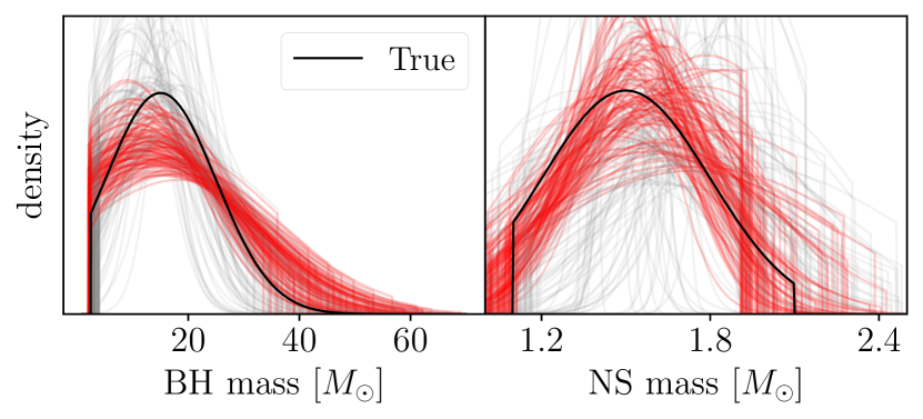
Figure 1: Constraints on the BH mass distribution (left) and the the NS mass distribution (right). The grey and red curves are draws from the prior and posterior, respectively. The black curve is the true input of our simulation.

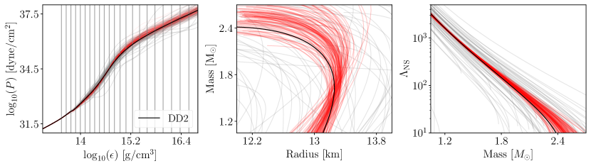
Figure 2: Constraints on (from left to right) the nuclear EOS, the NS mass-radius relationship and and the mass-$\Lambda$ relationship. The grey and red curves are draws from the prior and posterior, respectively. The black curve is the true input of our simulation. The gray vertical lines indicate the locations of our $24$ nodes.

Our population model parameters, $\Omega$, describe the mass distributions of BHs and NSs and the nuclear EOS. For the former, we use truncated normal distributions with the same parameters used in our simulations. The prior distributions for these parameters are listed in Table 1.

The prior for the EOS must be chosen more carefully, being defined on the space of (monotonically increasing) functions $p(\epsilon)$ which encode the dependence of pressure, $p$, on energy density, $\epsilon$. For numerical calculations we work with the logarithms of these two quantities, expressing $\epsilon$ in units of $\mathrm{MeV~{}fm^{-3}}$ and $p$ in units of $\mathrm{dyne~{}cm^{-2}}$. Simply adopting common flexible parameterizations such as a piece-wise polytrope [47] or spectral-decomposition [48] can, however, introduce undesirable implicit correlations [49, 50]. We hence build a more flexible Gaussian process (GP) prior for the (log) EOS [51, 52, 50]. This is defined by $n$ nodes, $\log_{10}(\epsilon_{1:n})$ and $\log_{10}(p_{1:n})$, indexed by $k\in\{1,2,\ldots,N\}$. This approach is strictly valid only in the $n\rightarrow\infty$ limit, but for the nuclear EOS we find that $n=24$ is sufficient for practical purposes. The positions of the nodes in log energy density, $\log_{10}(\epsilon_{1:n})$, are shown in Fig. 2. For the prior mean of the (log) pressure of the $k$’th node we set $\log_{10}(\bar{p}_{k})=\log_{10}[p_{\rm DD2}(\epsilon_{k})]$ as given by the DD2 EOS. Below an energy density of $19.7\,\mathrm{MeV~{}fm^{-3}}$, we force the GP to match DD2, i.e., conditioning the GP prior to match the better-known low density physics of the NS crust (as done in other EOS analyses). To encode the correlations between the pressure at different nodes we adopt a squared exponential GP kernel of the form $C_{k,k^{\prime}}=k_{1}\exp\{-[\log_{10}(\epsilon_{k})-\log_{10}(\epsilon_{k^{\prime}})]^{2}/(2\,k_{2}^{2})\}$, where the amplitude, $k_{1}$, and scale, $k_{2}$, become global nuisance parameters which are constrained by the node-to-node covariance of the simulated EOS.

We sample an EOS from this prior distribution by using a three step process. We first draw $\log_{10}(\mathbf{p})=\log_{10}(p_{1:n})$ from an $n$-dimensional multivariate normal distribution with mean $\log_{10}(\bar{\mathbf{p}})=\log_{10}(\bar{p}_{1:n})$ and covariance matrix $\mathbf{C}=C_{1:n,1:n}$. We then form a full EOS by using GP interpolation to transform the $\log_{10}[p(\epsilon)]$ at $n=24$ nodes onto a denser array of $2000$ nodes. This can produce models that are acausal or thermodynamically unstable [3]; these are removed using rejection sampling. For the implied $p(\epsilon)$, we solve the tidal and Tolman-Oppenheimer-Volkoff (TOV) equations to obtain $\Lambda(m)$, which is used in the evaluation of the Monte Carlo integral in the likelihood in Eq. 2.

Definition	Parameter	Prior
BH mass function mean	$\mu_{\rm BH}/\mathrm{M_{\odot}}$	${\rm U}(8,20)$
BH mass function width	$\sigma_{\rm BH}/\mathrm{M_{\odot}}$	${\rm U}(4,20)$
BH mass function minimum	$a_{\rm BH}/\mathrm{M_{\odot}}$	${\rm U}(2,4)$
BH mass function maximum	$b_{\rm BH}/\mathrm{M_{\odot}}$	${\rm U}(30,70)$
NS mass function mean	$\mu_{\rm NS}/\mathrm{M_{\odot}}$	${\rm U}(1.3,2.0)$
NS mass function width	$\sigma_{\rm NS}/\mathrm{M_{\odot}}$	${\rm U}(0.01,0.6)$
NS mass function minimum	$a_{\rm NS}/\mathrm{M_{\odot}}$	${\rm U}(0.9,1.4)$
NS mass function maximum	$b_{\rm NS}/\mathrm{M_{\odot}}$	${\rm U}(1.9,2.5)$
EOS GP amplitude	$\log(k_{1})$	${\rm U}(0.1,0.8)$
EOS GP scale	$k_{2}$	${\rm U}(0.2,1.0)$

Table 1: Population parameters and their prior distributions.

With this EOS parameterization, we have a total of 34 population parameters: the parameters of the BH and NS mass distributions; the GP kernel hyper-parameters; and the pressure at the $n=24$ EOS nodes. In Fig. 1 and Fig. 2, we show random draws from our full prior for different NS and BH properties. Our priors are summarized in Table 1. We obtain the posterior on these hyperparameters using the likelihood in Eq. 2, sampling from $P(\Omega|d_{1:N},I)$ using the nested sampler pymultinest [53, 54] implemented in Bilby [45, 43]. We evaluate the likelihood on a GPU using cupy to reduce the computational cost. The analysis steps from transforming the individual event posteriors, building a Gaussian mixture model density estimate, to producing posteriors on the hyperparameters takes $\mathcal{O}(1\,\mathrm{day})$ on a NVIDIA P100 GPU, limited primarily by the need to solve the TOV equations at every iteration of the likelihood.

Results. Following the methodology outlined above, we present the results from our EMGW-selected population of NSBH mergers. Our simulation recovers the input values for all parameters, indicating no bias in our analysis and that we have correctly accounted for selection effects.

In Fig. 1 and 2, we show the prior and posterior predictive distributions for the BH mass distribution $P(m_{\rm BH})$, the NS mass distribution $P(m_{\rm NS})$, the NS EOS (i.e., $p(\epsilon)$), and the mass-radius and the mass-$\Lambda$ curves. We again see that the true input of the simulation is recovered, indicating no bias in our analysis and correct accounting of selection effects in this projected representation of parameters. We measure the BH and NS mass distribution means with $40\%$ and $10\%$ precision ($68\%$ credible intervals), respectively. However, the high mass cut-off in the NS mass distribution and low-mass cut-off in the BH mass distribution are not constrained well, with significant overlap suggesting that a sample of this size will not be able to verify the existence of a mass gap between NSs and BHs, consistent with previous results [55, 56].

To quantify the constraining power on the nuclear EOS, we can consider the constraints on the tidal deformability and radius of a $1.4\,\mathrm{M_{\odot}}$ NS as ${697.58}_{-27.17}^{+41.17}$ and ${13.18}\pm 0.11~{}\rm{km}$ ($68\%$ credible interval), i.e., a precision of $10\%$ and $1.6\%$ respectively. Similarly, we can also constrain the maximum NS mass to be ${2.50}_{-0.14}^{+0.19}M_{\odot}$ ($68\%$ credible interval), i.e., a relative precision of $13\%$. The precision of each measurement is comparable to other state-of-the-art methods to constrain the behaviour of nuclear matter [e.g., 7, 57, 52], demonstrating the importance of constraints provided by observations of NSBHs.

Further, a significant benefit of our new GP-based EOS inference methodology is that it directly constrains the pressure at specific energy densities (the GP nodes) and the size and length scale parameters of correlations in $p(\epsilon$). Our simulations imply that the length scale of correlations (i.e., the smoothness) in $p(\epsilon)$ can be constrained to be $\geq~{}3.2\,\mathrm{MeV~{}fm^{-3}}$ with $90\%$ confidence, an important consideration for determining the size and location of putative phase transitions.

Conclusions. We have presented the constraints on the BH and NS mass distributions and the nuclear EOS that could be provided by a sample of multi-messenger NSBH events from $5\,\mathrm{years}$ of the A+ era GW observatories operating in tandem with large-scale optical surveys like LSST. Our EOS constraints come only from the GW data, with EM selection only serving to ensure a pure NSBH sample. Folding in the EOS dependence into the modeling of the EM counterpart could further improve constraints from such mergers [32]. Our EOS inference methodology also offers the ability to directly constrain structure in the EOS, an important consideration for probing the existence of phase transitions.

The precision of EOS constraints provided by such a sample of NSBH mergers are comparable to projected constraints from BNS mergers and better than constraints provided by NICER [57]. In particular, for $47$ multi-messenger NSBH events, we can obtain $1.6\%$ precision measurement on the radius of $1.4\,\mathrm{M_{\odot}}$ NS cf. $2\%$ constraint for $\sim 50$ BNS mergers for a similar equation of state and 3-detector GW network at design sensitivity [58]. Currently, the local rate of both BNS and NSBH mergers are highly uncertain [12]. However, the number of NSBH candidates currently outnumber BNS candidates, and this could conceivably continue given the former are detectable out to a larger volume. This study demonstrates the strong complementarity of NSBH mergers as a probe of the behavior of nuclear matter, especially given that it is unclear as yet which merger type will dominate future EMGW samples.

A number of improvements will be required to realize the promise of NSBH mergers. For example, the analysis of real observations will require a more sophisticated treatment of EM selection that incorporates viewing angle dependencies, the intrinsic diversity of EM counterpart signals [59], and real survey observing strategies [29], alongside improvements to physical models of EM counterparts to ensure that kilonovae from NSBH can be robustly identified. If GW observations alone could ensure a pure NSBH sample (i.e., by ruling out contamination from BNS or BBH mergers) [e.g., 60], this would remove the need for EM selection, dramatically increasing the number of observations available to constrain the EOS. Further, as constraints on the EOS are dominated by events with high SNR, a better understanding of waveform systematics in that regime will be essential [e.g., 61, 62, 13]. Finally, it may be promising to investigate building more physical relationships (such as density-dependent correlations seen in numerical EOS models) into EOS priors, while retaining the advantage of flexibility offered by GP modeling.

Software. This work used Bilby, available at https://git.ligo.org/lscsoft/bilby and Redback [63], available at https://github.com/nikhil-sarin/redback. Specific analysis scripts are available upon request.

Acknowledgments. We thank Alex Brown, Eric Thrane, Greg Ashton, and Shanika Galaudage for helpful discussions. We are grateful to the SEOBNR waveform modelers for making their waveforms public, without which this work would not have been possible. NS is supported by a Nordita Fellowship. Nordita is supported in part by NordForsk. This project has received funding from the European Research Council (ERC) under the European Union’s Horizon 2020 research and innovation programmes (grant agreement no. 101018897 CosmicExplorer) and by the research project grant ‘Fundamental physics from populations of compact object mergers’ funded by VR under Dnr 2021-04195. This work has benefitted from the research environment grant ‘Gravitational Radiation and Electromagnetic Astrophysical Transients (GREAT)’ funded by the Swedish Research Council (VR) under Dnr 2016-06012 and the research project grant ‘Gravity Meets Light’ funded by the Knut and Alice Wallenberg Foundation Dnr KAW 2019.0112. The work of HVP was additionally supported by the Göran Gustafsson Foundation for Research in Natural Sciences and Medicine. SMN is grateful for financial support from the Nederlandse Organisatie voor Wetenschappelijk Onderzoek (NWO) through the VIDI and Projectruimte grants. NS, HVP and DJM acknowledge the hospitality of the Aspen Center for Physics, which is supported by National Science Foundation grant PHY-1607611. The participation of HVP and DJM at the Aspen Center for Physics was supported by the Simons Foundation. This work used computing facilities provided by the OzSTAR national facility at Swinburne University of Technology. The OzSTAR program receives funding in part from the Astronomy National Collaborative Research Infrastructure Strategy (NCRIS) allocation provided by the Australian Government. This material is based upon work supported by NSF’s LIGO Laboratory which is a major facility fully funded by the National Science Foundation.

Author contributions. NS: conceptualization, methodology, software, investigation, validation, writing (original draft preparation). HVP: conceptualization, methodology, validation, writing (review & editing) DJM: conceptualization, methodology, writing (review & editing). JA: methodology, validation, writing (review & editing). SMN: conceptualization, writing (review & editing). SMF: conceptualization.

Appendix A Supplemental Material

Selected population. Here we present the impact of GW and EM selection on our population in Fig. 3. The predominant effect of the GW selection is to favor nearby mergers and face-on events, both of which produce a stronger GW signal. By contrast, the most significant impact of EM selection is on luminosity distance, mass ratio, chirp mass and BH spin, with lower chirp masses and higher spins leading to more favorable conditions for disrupting the NS, while the events must also be sufficiently nearby to produce a detectable EM transient.

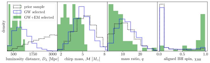
Figure 3: Distributions of a subset of parameters for our simulated population. In particular, luminosity distance $D_{L}$, chirp mass ${\cal{M}}$, mass ratio $q=m_{\rm BH}/m_{\rm NS}$, and the black hole spin $\chi_{\rm BH}$ of the binary. The black curves show the full simulated population, the blue curves show the GW selected population, and the green histograms show the multi-messenger (EM + GW) selected population.

Individual event posteriors. Here we present the posteriors from our individual event analysis and from the full population analysis. In Fig. 4 we show the constraints on the mass and radius from the individual events. The $3\sigma$ credible regions for all events include the true/input value, giving confidence in an unbiased recovery. Fig. 4 also demonstrates that the dominant constraints on the $\Lambda(m)$ curve are provided by the loudest GW events, consistent with previous work [64, 40]. This highlights that the constraints on the nuclear EOS will be highly dependent on the ability to detect a handful of exceptionally loud events, as opposed to many weak events, stressing the need for understanding waveform systematics for high SNR systems.

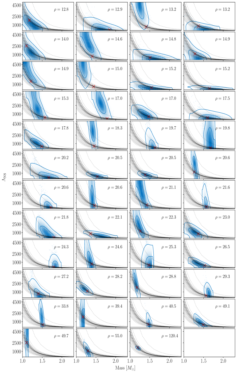
Figure 4: Constraints on the mass and tidal deformability of neutron stars in our all events with the blue shaded region indicating the $50$ and $90\%$ credible regions and the red cross showing the input value. The annotation indicates the network matched-filter SNR of our events, while the gray curves indicate random draws from the GP prior.

References

- Baym et al. [2018] G. Baym, T. Hatsuda, T. Kojo, P. D. Powell, and et al., From hadrons to quarks in neutron stars: a review, Reports on Progress in Physics 81, 056902 (2018), arXiv:1707.04966 [astro-ph.HE] .
- Sorensen et al. [2023] A. Sorensen, K. Agarwal, K. W. Brown, Z. Chajecki, and et al., Dense Nuclear Matter Equation of State from Heavy-Ion Collisions, arXiv e-prints , arXiv:2301.13253 (2023), arXiv:2301.13253 [nucl-th] .
- Lattimer and Prakash [2001] J. M. Lattimer and M. Prakash, Neutron Star Structure and the Equation of State, ApJ 550, 426 (2001), arXiv:astro-ph/0002232 [astro-ph] .
- Greif et al. [2020] S. K. Greif, K. Hebeler, J. M. Lattimer, C. J. Pethick, and et al., Equation of State Constraints from Nuclear Physics, Neutron Star Masses, and Future Moment of Inertia Measurements, ApJ 901, 155 (2020), arXiv:2005.14164 [astro-ph.HE] .
- Demorest et al. [2010] P. B. Demorest, T. Pennucci, S. M. Ransom, M. S. E. Roberts, and et al., A two-solar-mass neutron star measured using Shapiro delay, Nature 467, 1081 (2010), arXiv:1010.5788 [astro-ph.HE] .
- Cromartie et al. [2020] H. T. Cromartie, E. Fonseca, S. M. Ransom, P. B. Demorest, and et al., Relativistic Shapiro delay measurements of an extremely massive millisecond pulsar, Nature Astronomy 4, 72 (2020), arXiv:1904.06759 [astro-ph.HE] .
- Riley et al. [2019] T. E. Riley, A. L. Watts, S. Bogdanov, P. S. Ray, and et al., A NICER View of PSR J0030+0451: Millisecond Pulsar Parameter Estimation, ApJ 887, L21 (2019), arXiv:1912.05702 [astro-ph.HE] .
- Abbott et al. [2017a] B. P. Abbott, R. Abbott, T. D. Abbott, F. Acernese, K. Ackley, et al., GW170817: Observation of Gravitational Waves from a Binary Neutron Star Inspiral, Phys. Rev. Lett. 119, 161101 (2017a).
- Abbott et al. [2017b] B. P. Abbott, R. Abbott, T. D. Abbott, F. Acernese, K. Ackley, C. Adams, T. Adams, P. Addesso, et al., Multi-messenger Observations of a Binary Neutron Star Merger, ApJ 848, L12 (2017b), arXiv:1710.05833 [astro-ph.HE] .
- Abbott et al. [2019] B. P. Abbott, R. Abbott, T. D. Abbott, F. Acernese, K. Ackley, et al., Properties of the Binary Neutron Star Merger GW170817, \prx 9, 011001 (2019).
- Abbott et al. [2018] B. P. Abbott, R. Abbott, T. D. Abbott, F. Acernese, and et al., GW170817: Measurements of Neutron Star Radii and Equation of State, Phys. Rev. Lett. 121, 161101 (2018), arXiv:1805.11581 [gr-qc] .
- The LIGO Scientific Collaboration et al. [2021] The LIGO Scientific Collaboration, the Virgo Collaboration, the KAGRA Collaboration, R. Abbott, and et al., The population of merging compact binaries inferred using gravitational waves through GWTC-3, arXiv e-prints , arXiv:2111.03634 (2021), arXiv:2111.03634 [astro-ph.HE] .
- Huang et al. [2021] Y. Huang, C.-J. Haster, S. Vitale, V. Varma, and et al., Statistical and systematic uncertainties in extracting the source properties of neutron star-black hole binaries with gravitational waves, Phys. Rev. D 103, 083001 (2021), arXiv:2005.11850 [gr-qc] .
- Clarke et al. [2023] T. A. Clarke, L. Chastain, P. D. Lasky, and E. Thrane, Nuclear Physics with Gravitational Waves from Neutron Stars Disrupted by Black Holes, ApJ 949, L6 (2023), arXiv:2302.09711 [gr-qc] .
- Abbott et al. [2021] R. Abbott, T. D. Abbott, S. Abraham, F. Acernese, and et al., Observation of Gravitational Waves from Two Neutron Star-Black Hole Coalescences, ApJ 915, L5 (2021), arXiv:2106.15163 [astro-ph.HE] .
- Broekgaarden et al. [2021] F. S. Broekgaarden, E. Berger, C. J. Neijssel, A. Vigna-Gómez, and et al., Impact of massive binary star and cosmic evolution on gravitational wave observations I: black hole-neutron star mergers, MNRAS 508, 5028 (2021), arXiv:2103.02608 [astro-ph.HE] .
- Hempel and Schaffner-Bielich [2010] M. Hempel and J. Schaffner-Bielich, A statistical model for a complete supernova equation of state, Nucl. Phys. A 837, 210 (2010), arXiv:0911.4073 [nucl-th] .
- Chattopadhyay et al. [2021] D. Chattopadhyay, S. Stevenson, J. R. Hurley, M. Bailes, and et al., Modelling neutron star-black hole binaries: future pulsar surveys and gravitational wave detectors, MNRAS 504, 3682 (2021), arXiv:2011.13503 [astro-ph.HE] .
- Abbott et al. [2020] B. P. Abbott, R. Abbott, T. D. Abbott, S. Abraham, F. Acernese, K. Ackley, C. Adams, V. B. Adya, et al., Prospects for observing and localizing gravitational-wave transients with Advanced LIGO, Advanced Virgo and KAGRA, Living Reviews in Relativity 23, 3 (2020).
- Aasi et al. [2015] J. Aasi et al., Advanced LIGO, CQG 32, 074001 (2015).
- Acernese et al. [2015] F. Acernese et al., Advanced Virgo: a second-generation interferometric gravitational wave detector, 32, 024001 (2015).
- Akutsu et al. [2019] T. Akutsu, M. Ando, K. Arai, and et al., KAGRA: 2.5 generation interferometric gravitational wave detector, Nature Astronomy 3, 35 (2019), arXiv:1811.08079 [gr-qc] .
- Saleem et al. [2022] M. Saleem, J. Rana, V. Gayathri, A. Vijaykumar, and et al., The science case for LIGO-India, Classical and Quantum Gravity 39, 025004 (2022), arXiv:2105.01716 [gr-qc] .
- Gupta et al. [2023] I. Gupta, S. Borhanian, A. Dhani, D. Chattopadhyay, and et al., Neutron star-black hole mergers in next generation gravitational-wave observatories, Phys. Rev. D 107, 124007 (2023), arXiv:2301.08763 [gr-qc] .
- Matas et al. [2020] A. Matas, T. Dietrich, A. Buonanno, T. Hinderer, and et al., Aligned-spin neutron-star-black-hole waveform model based on the effective-one-body approach and numerical-relativity simulations, Phys. Rev. D 102, 043023 (2020), arXiv:2004.10001 [gr-qc] .
- Foucart et al. [2018] F. Foucart, T. Hinderer, and S. Nissanke, Remnant baryon mass in neutron star-black hole mergers: Predictions for binary neutron star mimickers and rapidly spinning black holes, Phys. Rev. D 98, 081501 (2018).
- Zappa et al. [2019] F. Zappa, S. Bernuzzi, F. Pannarale, M. Mapelli, and et al., Black-Hole Remnants from Black-Hole-Neutron-Star Mergers, Phys. Rev. Lett. 123, 041102 (2019), arXiv:1903.11622 [gr-qc] .
- Ivezić et al. [2019] Ž. Ivezić, S. M. Kahn, J. A. Tyson, B. Abel, and et al., LSST: From Science Drivers to Reference Design and Anticipated Data Products, ApJ 873, 111 (2019), arXiv:0805.2366 [astro-ph] .
- Andreoni et al. [2022] I. Andreoni, R. Margutti, O. S. Salafia, B. Parazin, and et al., Target-of-opportunity Observations of Gravitational-wave Events with Vera C. Rubin Observatory, ApJS 260, 18 (2022), arXiv:2111.01945 [astro-ph.HE] .
- Radice et al. [2018] D. Radice, A. Perego, F. Zappa, and S. Bernuzzi, GW170817: Joint Constraint on the Neutron Star Equation of State from Multimessenger Observations, ApJ 852, L29 (2018), arXiv:1711.03647 [astro-ph.HE] .
- Hinderer et al. [2019] T. Hinderer, S. Nissanke, F. Foucart, K. Hotokezaka, and et al., Distinguishing the nature of comparable-mass neutron star binary systems with multimessenger observations: GW170817 case study, Phys. Rev. D 100, 063021 (2019), arXiv:1808.03836 [astro-ph.HE] .
- Raaijmakers et al. [2021] G. Raaijmakers, S. Nissanke, F. Foucart, M. M. Kasliwal, and et al., The Challenges Ahead for Multimessenger Analyses of Gravitational Waves and Kilonova: A Case Study on GW190425, ApJ 922, 269 (2021), arXiv:2102.11569 [astro-ph.HE] .
- Barbieri et al. [2019] C. Barbieri, O. S. Salafia, A. Perego, M. Colpi, and G. Ghirlanda, Light-curve models of black hole - neutron star mergers: steps towards a multi-messenger parameter estimation, A&A 625, A152 (2019), arXiv:1903.04543 [astro-ph.HE] .
- Sarin et al. [2022] N. Sarin, P. D. Lasky, F. H. Vivanco, S. P. Stevenson, and et al., Linking the rates of neutron star binaries and short gamma-ray bursts, Phys. Rev. D 105, 083004 (2022), arXiv:2201.08491 [astro-ph.HE] .
- Biscoveanu et al. [2023] S. Biscoveanu, P. Landry, and S. Vitale, Population properties and multimessenger prospects of neutron star-black hole mergers following GWTC-3, MNRAS 518, 5298 (2023), arXiv:2207.01568 [astro-ph.HE] .
- Setzer et al. [2019] C. N. Setzer, R. Biswas, H. V. Peiris, S. Rosswog, and et al., Serendipitous discoveries of kilonovae in the LSST main survey: maximizing detections of sub-threshold gravitational wave events, MNRAS 485, 4260 (2019), arXiv:1812.10492 [astro-ph.IM] .
- Zhu et al. [2020] J.-P. Zhu, Y.-P. Yang, L.-D. Liu, Y. Huang, B. Zhang, Z. Li, Y.-W. Yu, and H. Gao, Kilonova Emission from Black Hole-Neutron Star Mergers. I. Viewing-angle-dependent Lightcurves, ApJ 897, 20 (2020), arXiv:2003.06733 [astro-ph.HE] .
- Almualla et al. [2021] M. Almualla, S. Anand, M. W. Coughlin, T. Dietrich, and et al., Optimizing serendipitous detections of kilonovae: cadence and filter selection, MNRAS 504, 2822 (2021), arXiv:2011.10421 [astro-ph.HE] .
- Henkel et al. [2023] A. Henkel, F. Foucart, G. Raaijmakers, and S. Nissanke, Study of the agreement between binary neutron star ejecta models derived from numerical relativity simulations, Phys. Rev. D 107, 063028 (2023), arXiv:2207.07658 [astro-ph.HE] .
- Golomb and Talbot [2022] J. Golomb and C. Talbot, Hierarchical Inference of Binary Neutron Star Mass Distribution and Equation of State with Gravitational Waves, ApJ 926, 79 (2022), arXiv:2106.15745 [astro-ph.HE] .
- Mandel et al. [2019] I. Mandel, W. M. Farr, and J. R. Gair, Extracting distribution parameters from multiple uncertain observations with selection biases, MNRAS 486, 1086 (2019), arXiv:1809.02063 [physics.data-an] .
- Vitale et al. [2022] S. Vitale, D. Gerosa, W. M. Farr, and S. R. Taylor, Inferring the Properties of a Population of Compact Binaries in Presence of Selection Effects, in Handbook of Gravitational Wave Astronomy (2022) p. 45.
- Romero-Shaw et al. [2020] I. M. Romero-Shaw, C. Talbot, S. Biscoveanu, V. D’Emilio, G. Ashton, C. P. L. Berry, S. Coughlin, S. Galaudage, C. Hoy, M. Hübner, K. S. Phukon, M. Pitkin, M. Rizzo, N. Sarin, R. Smith, S. Stevenson, A. Vajpeyi, M. Arène, K. Athar, S. Banagiri, N. Bose, M. Carney, K. Chatziioannou, J. A. Clark, M. Colleoni, R. Cotesta, B. Edelman, H. Estellés, C. García-Quirós, A. Ghosh, R. Green, C. J. Haster, S. Husa, D. Keitel, A. X. Kim, F. Hernandez-Vivanco, I. Magaña Hernandez, C. Karathanasis, P. D. Lasky, N. De Lillo, M. E. Lower, D. Macleod, M. Mateu-Lucena, A. Miller, M. Millhouse, S. Morisaki, S. H. Oh, S. Ossokine, E. Payne, J. Powell, G. Pratten, M. Pürrer, A. Ramos-Buades, V. Raymond, E. Thrane, J. Veitch, D. Williams, M. J. Williams, and L. Xiao, Bayesian inference for compact binary coalescences with BILBY: validation and application to the first LIGO-Virgo gravitational-wave transient catalogue, MNRAS 499, 3295 (2020), arXiv:2006.00714 [astro-ph.IM] .
- Foreman-Mackey et al. [2013] D. Foreman-Mackey, D. W. Hogg, D. Lang, and J. Goodman, emcee: The MCMC Hammer, PASP 125, 306 (2013), arXiv:1202.3665 [astro-ph.IM] .
- Ashton et al. [2019] G. Ashton, M. Hübner, P. D. Lasky, C. Talbot, K. Ackley, S. Biscoveanu, Q. Chu, A. Divakarla, P. J. Easter, B. Goncharov, F. Hernandez Vivanco, J. Harms, M. E. Lower, G. D. Meadors, D. Melchor, E. Payne, M. D. Pitkin, J. Powell, N. Sarin, R. J. E. Smith, and E. Thrane, BILBY: A User-friendly Bayesian Inference Library for Gravitational-wave Astronomy, ApJS 241, 27 (2019).
- Dietrich et al. [2019] T. Dietrich, A. Samajdar, S. Khan, N. K. Johnson-McDaniel, and et al., Improving the NRTidal model for binary neutron star systems, Phys. Rev. D 100, 044003 (2019), arXiv:1905.06011 [gr-qc] .
- Read et al. [2009] J. S. Read, C. Markakis, M. Shibata, K. Uryū, and et al., Measuring the neutron star equation of state with gravitational wave observations, Phys. Rev. D 79, 124033 (2009), arXiv:0901.3258 [gr-qc] .
- Lindblom [2010] L. Lindblom, Spectral representations of neutron-star equations of state, Phys. Rev. D 82, 103011 (2010), arXiv:1009.0738 [astro-ph.HE] .
- Raaijmakers et al. [2018] G. Raaijmakers, T. E. Riley, and A. L. Watts, A pitfall of piecewise-polytropic equation of state inference, MNRAS 478, 2177 (2018), arXiv:1804.09087 [astro-ph.HE] .
- Legred et al. [2022] I. Legred, K. Chatziioannou, R. Essick, and P. Landry, Implicit correlations within phenomenological parametric models of the neutron star equation of state, Phys. Rev. D 105, 043016 (2022), arXiv:2201.06791 [astro-ph.HE] .
- Landry and Essick [2019] P. Landry and R. Essick, Nonparametric inference of the neutron star equation of state from gravitational wave observations, Phys. Rev. D 99, 084049 (2019), arXiv:1811.12529 [gr-qc] .
- Essick et al. [2020] R. Essick, P. Landry, and D. E. Holz, Nonparametric inference of neutron star composition, equation of state, and maximum mass with GW170817, Phys. Rev. D 101, 063007 (2020), arXiv:1910.09740 [astro-ph.HE] .
- Feroz et al. [2009] F. Feroz, M. P. Hobson, and M. Bridges, MULTINEST: an efficient and robust Bayesian inference tool for cosmology and particle physics, MNRAS 398, 1601 (2009), arXiv:0809.3437 [astro-ph] .
- Buchner [2016] J. Buchner, PyMultiNest: Python interface for MultiNest, Astrophysics Source Code Library, record ascl:1606.005 (2016), ascl:1606.005 .
- Alsing et al. [2018] J. Alsing, H. O. Silva, and E. Berti, Evidence for a maximum mass cut-off in the neutron star mass distribution and constraints on the equation of state, MNRAS 478, 1377 (2018), arXiv:1709.07889 [astro-ph.HE] .
- Ye and Fishbach [2022] C. Ye and M. Fishbach, Inferring the Neutron Star Maximum Mass and Lower Mass Gap in Neutron Star-Black Hole Systems with Spin, ApJ 937, 73 (2022), arXiv:2202.05164 [astro-ph.HE] .
- Raaijmakers et al. [2019] G. Raaijmakers, T. E. Riley, A. L. Watts, S. K. Greif, and et al., A Nicer View of PSR J0030+0451: Implications for the Dense Matter Equation of State, ApJ 887, L22 (2019), arXiv:1912.05703 [astro-ph.HE] .
- Finstad et al. [2022] D. Finstad, L. V. White, and D. A. Brown, Prospects for a precise equation of state measurement from Advanced LIGO and Cosmic Explorer, arXiv e-prints , arXiv:2211.01396 (2022), arXiv:2211.01396 [astro-ph.HE] .
- Setzer et al. [2023] C. N. Setzer, H. V. Peiris, O. Korobkin, and S. Rosswog, Modelling populations of kilonovae, MNRAS 520, 2829 (2023), arXiv:2205.12286 [astro-ph.HE] .
- Brown et al. [2022] S. M. Brown, C. D. Capano, and B. Krishnan, Using Gravitational Waves to Distinguish between Neutron Stars and Black Holes in Compact Binary Mergers, ApJ 941, 98 (2022), arXiv:2105.03485 [gr-qc] .
- Pürrer and Haster [2020] M. Pürrer and C.-J. Haster, Gravitational waveform accuracy requirements for future ground-based detectors, Physical Review Research 2, 023151 (2020), arXiv:1912.10055 [gr-qc] .
- Gamba et al. [2021] R. Gamba, M. Breschi, S. Bernuzzi, M. Agathos, and et al., Waveform systematics in the gravitational-wave inference of tidal parameters and equation of state from binary neutron-star signals, Phys. Rev. D 103, 124015 (2021), arXiv:2009.08467 [gr-qc] .
- Sarin et al. [2023] N. Sarin, M. Hübner, C. M. B. Omand, C. N. Setzer, and et al., Redback: A Bayesian inference software package for electromagnetic transients, arXiv e-prints , arXiv:2308.12806 (2023), arXiv:2308.12806 [astro-ph.HE] .
- Hernandez Vivanco et al. [2019] F. Hernandez Vivanco, R. Smith, E. Thrane, P. D. Lasky, and et al., Measuring the neutron star equation of state with gravitational waves: The first forty binary neutron star merger observations, Phys. Rev. D 100, 103009 (2019), arXiv:1909.02698 [gr-qc] .