Real-time error mitigation for variational optimization on quantum hardware

Abstract

In this work we put forward the inclusion of error mitigation routines in the process of training Variational Quantum Circuit (VQC) models. In detail, we define a Real Time Quantum Error Mitigation (RTQEM) algorithm to assist in fitting functions on quantum chips with VQCs. While state-of-the-art QEM methods cannot address the exponential loss concentration induced by noise in current devices, we demonstrate that our RTQEM routine can enhance VQCs’ trainability by reducing the corruption of the loss function. We tested the algorithm by simulating and deploying the fit of a monodimensional u-Quark Parton Distribution Function (PDF) on a superconducting single-qubit device, and we further analyzed the scalability of the proposed technique by simulating a multidimensional fit with up to 8 qubits.

In the era of Noisy Intermediate Scale Quantum (NISQ) [1, 2] devices, Variational Quantum Algorithms (VQA) are the Quantum Machine Learning (QML) models that appear more promising in the near future. They have several concrete applications already validated, such as electronic structure modelization in quantum chemistry [3, 4, 5, 6], for instance. Different VQA ansätze have been proposed, such as the QAOA [7], but they all share as foundation a Variational Quantum Circuit (VQC) consisting of several parameterized gates whose parameters are updated during training.

Hardware errors and large execution times corrupt the landscape in various ways, such as changing the position of the minimum or the optimal value of the loss function, hindering NISQ [1, 2] devices’ applicability in practice for certain algorithms. Furthermore, VQC models are known to suffer from the presence of Noise-Induced Barren Plateaus (NIBPs) [8] in the optimization space, leading to vanishing gradients. NIBPs are fundamentally different from the noise-free barren plateaus discussed in Refs [9, 10, 11, 12, 13, 14]. In fact, approaches designed to tackle noise-free barren plateaus do not seem to effectively address the issues posed by NIBPs [8].

To overcome these limitations we either have to build fault-tolerant architectures carrying a usable amount of logical qubits, or exploit the available NISQ hardware by mitigating its results from the noise. While the first solution might require significant technical advances, the second one is often achieved with the help of quantum error mitigation (QEM) [15]. Exponential loss concentration cannot be resolved with error mitigation [16], but it is possible to improve trainability by attempting to reduce the loss corruption. Therefore, we define here an algorithm to perform Real-Time Quantum Error Mitigation (RTQEM) alongside a VQA-based QML training process.

In this work, we use the Importance Clifford Sampling (ISC) method [17], a learning-based quantum error mitigation procedure [18]. The core business of the learning-based QEM techniques is to approximate the noise with a parametric map which, once learned, can be used to clean the noisy results [19, 20, 21, 22, 23]. Linear maps have the potential to improve overall trainability by addressing challenges imposed by loss corruptions while not affecting loss concentration itself [16]. The map’s parameters are learned during the QML training every time the noise changes above a certain arbitrarily set threshold.

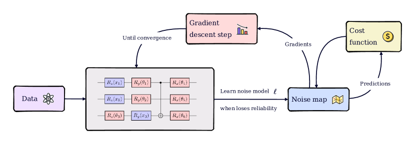
Figure 1: The RTQEM pipeline involves training a variational quantum circuit on a noisy quantum device using a gradient descent method enhanced with error mitigation. Specifically, the ICS algorithm is used to learn a noise map to mitigate both the gradients and the final predictions. If the noise changes above a certain threshold, the noise map is re-learned.

We apply the RTQEM strategy to a series of mono-dimensional and multi-dimensional regression problems. Firstly, we train a VQC to tackle a particularly interesting High Energy Physics (HEP) problem: determining the Parton Distribution Function (PDF) of the $u$-quark, one of the proton contents. In a second step, we define a multi-dimensional target to study the impact of the RTQEM procedure when the VQA involves an increasing number of qubits.

Data re-uploading [24] is used to encode data into the model, while we implement a hardware-compatible Adam [25] optimizer for the training. We calculate gradients with respect to the variational parameters using the Parameter Shift Rule [26, 27] (PSR). This optimization scheme is ideal for studying the performance of RTQEM, as the PSR formulas require a number of circuits to be executed which scales linearly with the number of parameters. The greater the number of executions, the better our algorithm must be to enable training of the model.

This setup is then used to perform the full $u$-quark PDF fit on two different superconducting quantum devices hosted in the Quantum Research Center (QRC) of the Technology Innovation Institute (TII).

The whole work has been realized using the Qibo framework, which offers Qibo [28, 29, 30, 31] as high-level language API to write quantum computing algorithms, Qibolab [32, 33, 34] as quantum control tool and Qibocal [35, 36, 37] to perform quantum characterization and calibration routines.

The outline is as follows. In Section I we summarize the process of quantum computing with the VQC paradigm, providing also details about the ansatz and the PSR rule we make use of to train the model. In Section II, we discuss the impact of noise on the training process and provide an overview of the error mitigation strategy we employed to counteract these effects. Finally, we report the results of our experiments both with noisy simulations and real superconducting qubits deployment in Section IV.

I Methodology

I.1 A snapshot of Quantum Machine Learning

In the following we are going to consider Supervised Machine Learning problems for simplicity, but what presented here can be easily extended to other Machine Learning (ML) paradigms in the quantum computation context. Quantum Machine Learning (QML) arises when using Quantum Computing (QC) tools to tackle ML problems [38, 39, 26].

In the classical scenario, given an $n$-dimensional input variable $\bm{x}$, a parametric model is requested to estimate a target variable $y$, which is related to $\bm{x}=(x_{1},\ldots,x_{n})$ through some hidden law $y=g(\bm{x})$. The model estimations $y_{\rm est}$ are then compared with some measured ground truth data $y_{\rm meas}$ by evaluating a loss function $J(y_{\rm est},y_{\rm meas})$, which quantifies the capability of the model to provide an estimate of the underlying law $g$. We consider the output variable $y$ as mono-dimensional for simplicity, but in general it can be multi-dimensional. The variational parameters $\bm{\theta}$ of the model are then optimized to minimize (or maximize) the loss function $J$, leading, in turn, to better predictions $y_{\rm est}$.

In Quantum Machine Learning, we translate this paradigm to the language of quantum computing. In particular, parametric quantum gates, such as rotations, are used to build Variational Quantum Circuits (VQC) [40], which can be used as parametric models in the machine learning process. Once a parametric circuit $\mathcal{U}(\theta)$ is defined, it can be applied to a prepared initial state $\ket{\psi_{0}}$ of a quantum system to obtain the final state $\ket{\psi_{f}}$, which is used to evaluate the expected value of an arbitrary chosen observable $\mathcal{O}$,

$$f(\bm{\theta})_{\mathcal{O}}=\braket{\psi_{0}}{\,\mathcal{U}^{\dagger}(\bm{\theta})\mathcal{O}\,\mathcal{U}(\bm{\theta})}{\psi_{0}}\ .$$ (1)

Various methods exist to embed input data into a QML process [41, 42, 43]; in this work, we employ the re-uploading strategy [24]. The estimates of $y$ can be obtained by calculating expected values of the form (1). Finally, the circuit’s parameters are optimized to minimize (or maximize) a loss function $J$, pushing $f$ as close as possible to the unknown law $g$.

I.2 A variational circuit with data-reuploading

The data-reuploading [24] method is built by defining a parameterized layer made of fundamental uploading gates which accepts the input data $\bm{x}$ to be uploaded. Then, the re-uploading of the variable is achieved by building a circuit composed of a sequence of uploading layers.

[row sep = 2] $\ket{0}$ & L(x_1— θ_1,1) 1  ⋯  L(x_1— θ_l,1) 1
$\ket{0}$ L(x_2— θ_1,2) 1  ⋯  L(x_2— θ_l,2) 1
$\ket{0}$ L(x_3— θ_1,3) 1  ⋯  L(x_3— θ_l,3) 1
$\ket{0}$ L(x_4— θ_1,4) 1  ⋯  L(x_4— θ_l,4) 1
$\ket{0}$ L(x_n— θ_1,n) -4  ⋯  L(x_n— θ_l,n) -4

Figure 2: Circuit ansatz to reupload the data $\bm{x}$ with $n$ qubits and $l$ layers.

Inspired by [44], we build our ansatz by defining the following fundamental uploading gate,

$$L(x_{j}|\bm{\theta}_{l,j})=R_{z}(\theta_{3}\,x_{j}+\theta_{4})R_{y}(\theta_{1}\,\kappa(x_{j})+\theta_{2})\ ,$$ (2)

where $x_{j}$ is the $j$-th component of the input data and with $\bm{\theta}_{l,j}$ we denote the four-parameters vector composing the gate which uploads $x_{j}$ at the ansatz layer $l$. The information $x_{j}$ is uploaded twice in each $L$, first in the $R_{z}$ and second in the $R_{y}$ through an activation function $\kappa(x_{j})$. To embed the $n$ components of $\bm{x}$ into the ansatz, we build a $n$-qubit circuit $\mathcal{U}$ based on the Hardware Efficient Ansatz, where the single-qubit gates are the fundamental uploading gates, and entanglement is generated with CNOT gates, as shown in Fig. 2. We calculate $f$ (1) as the expected value of the Pauli observable $\sigma_{z}^{\otimes n}$ on the final state $\mathcal{U}\left(\ket{0}^{\otimes n}\right)$.

I.3 Gradient descent on hardware

Gradient-based optimizers [45, 25, 46, 47] are commonly employed in machine learning problems, particularly when using Neural Networks [48] (NNs) as models. In the QML context, VQCs are utilized to construct Quantum Neural Networks [49], which serve as quantum analogs of classical NNs. Consequently, we are naturally led to believe that methods based on gradient calculation could be effective.

I.3.1 The parameter shift rule

In order to perform a gradient descent on a NISQ device we need a method that is robust to noise and executable on hardware. This cannot be done as in the classical case following a back-propagation [45] of the information through the network. We would need to know the $f$ values during the propagation, but accessing this information would collapse the quantum state. Moreover, standard finite-differences methods are not applicable due to the shot noise when executing the circuit a finite number of times. An alternative method is the so called Parameter Shift Rule [50, 27, 51, 52, 53] (PSR), which enables the evaluation of quantum gradients directly on the hardware [27]. Given $f$ as introduced in (1) and considering a single parameter $\mu\in\bm{\theta}$ affecting a single gate whose hermitian generator has at most two eigenvalues, the PSR allows for the calculation

$$\partial_{\mu}f=r\bigl{(}f(\mu^{+})-f(\mu^{-})\bigr{)}\ ,$$ (3)

where $\pm r$ are the generator eigenvalues, $\mu^{\pm}=\mu\pm s$ and $s=-\pi/4r$. In other words, the derivative is calculated by executing twice the same circuit $\mathcal{U}(\bm{\theta})$ in which the parameter $\mu$ is shifted backward and forward of $s$. A remarkable case of the PSR involves rotation gates, for which we have $r=1/2$ and $s=\pi/2$ [26].

I.3.2 Evaluating gradients of a re-uploading model

In order to perform a gradient-based optimization, we first need to calculate the gradient of a loss function $J$ with respect to the variational parameters of the model. Then, the derivatives are used to perform an optimization step in the parameters’ space by following the steepest direction of the gradient,

$$\bm{\theta}_{t+1}=\bm{\theta}_{t}-\eta\nabla J(\bm{\theta}_{i})\ ,$$ (4)

where $\eta$ is the learning rate of the gradient descent algorithm. Since our QML model is a circuit in which the variational parameters are rotation angles, such derivatives can be estimated by the PSR (3). However, even in the simplest case, this kind of procedure can be computationally expensive, since for each parameter we need two evaluations of $f$, as illustrated in (3). Given a VQC with $p$ variational parameters, a training set size of $N_{\rm data}$, and a budget of $N_{\rm shots}$ for each function evaluation, the total computational cost amounts to $2pN_{\rm shots}N_{\rm data}$ circuit executions. This high number of evaluation is useful for testing the effectiveness of error mitigation routines, which can be applied to every function evaluation of the algorithm. We followed the same optimization strategy described in [54, 55], defining a Mean-Squared Error loss function,

$$J_{\rm mse}(\bm{x}^{i}|\bm{\theta})=\frac{1}{N_{\rm data}}\sum_{i}^{N_{\rm data}}\bigl{[}f(\bm{x}^{i},\bm{\theta})-g(\bm{x}^{i})\bigr{]}^{2}\ ,$$ (5)

where the superscript denotes the $i$-th variable $\bm{x}$ of the dataset. Note that this differs from the subscripts used so far to denote the components of the variable $\bm{x}$.

Our total execution time is dominated by the effect of circuit switching and network latency costs rather than shot cost. Therefore, we prefer to reduce the number of iterations at the expense of increasing the number of shots per iteration. In this context, the Adam [25] optimizer stands out due to its robustness when dealing with complex parameters landscapes.

II Noise on quantum hardware

Recognizing the impact of noise on the optimization landscape is crucial in practical quantum computing implementations. In the presence of a general class of local noise models, for many important ansätzes such as Hardware Efficient Ansatz (HEA), the gradient decreases exponentially with the depth of the circuit $d$. Typically, $d$ scales polynomially with the number of qubits $n$, causing the gradient to decrease exponentially in $n$. This phenomenon is referred to as a Noise-Induced Barren Plateau (NIBP) [56]. NIBPs can be seen as a consequence of the loss function converging around the value associated with the maximally mixed state. Furthermore, noise can corrupt the loss landscape in various ways such as changing the position of the minimum.

In order to quantify these effects, we consider a noise model composed of local Pauli channels acting on qubit $j$ before and after each layer of our ansatz,

$$\mathcal{P}_{j}(\sigma)=q_{j}\sigma\,$$ (6)

where $-1<q_{x},q_{y},q_{z}<1$ and $\sigma$ denotes the local Pauli operators $\{\sigma_{x},\sigma_{y},\sigma_{z}\}$. The overall channel is $\mathcal{P}=\bigotimes_{j}^{N}\mathcal{P}_{j}$. We also include symmetric readout noise $\mathcal{M}$ made of single-qubit bit-flip channels with bit-flip probability $(1-q_{M})/2$. This results in the noisy expectation value,

$$f_{\text{noisy}}=\operatorname{Tr}\bigl{[}\sigma_{z}^{\otimes n}\left(\mathcal{M}\circ\mathcal{P}\circ L_{l}\circ\cdots\circ L_{1}\circ\mathcal{P}\right)(\ket{\psi_{0}}\bra{\psi_{0}})\bigr{]}\ .$$ (7)

The NIBP translates into a concentration of the expectation value around $0$ [56],

$$\absolutevalue{f_{\text{noisy}}}<2q_{M}^{n}q^{2l+2}\left(1-\frac{1}{2^{n}}\right)\ .$$ (8)

Certain loss functions exhibit noise resilience, i.e. their minimum remains in the same position under the influence of certain noise models, even though its value may change. Contrarily, our loss function (5) is not noise resistant. We aim to explore the extent to which it is possible to mitigate the noise and enhance the training process of VQCs with non-resistant loss functions.

II.1 Error Mitigation

Recent research [57, 58, 59, 60, 61, 62] has focused on developing methods to define unbiased estimators of the ideal expected values leveraging the knowledge about the noise that we can extract from the hardware. However, these estimators are also affected by exponential loss concentration, implying that NIBPs cannot be resolved without requiring exponential resources through error mitigation [16].

In the regime where loss concentration is not severe, it is also not straightforward for error mitigation to improve the resolvability of the noisy loss landscape, thus alleviating exponential concentration.

The variance of the error-mitigated estimators is typically higher than that of the mean estimator [63], setting up a trade-off between the improvement due to bias reduction and the worsening caused by increased variance. While most methods have a negative impact on resolvability, linear ansatz methods [19, 17, 20, 21, 22, 23] show potential due to their neutral impact under global depolarizing noise [16]. Among all of them, Importance Clifford Sampling [17] stands out for its ability to handle single qubit dependent noise, its scalability, and its resource cost.

II.1.1 Importance Clifford Sampling (ICS)

Suppose we want to estimate the expected value of an observable $\mathcal{O}$ for the state $\rho$ prepared by a quantum circuit $\mathcal{C}^{0}$. In a realistic situation we are going to obtain a noisy expected value $\langle\mathcal{O}\rangle_{\rm noisy}^{0}$ different from the true one $\langle\mathcal{O}\rangle^{0}$. The idea behind Importance Clifford Sampling (ICS) is to generate a set of $m$ training Clifford circuits $\mathcal{S}=\big{\{}\mathcal{C}^{i}\big{\}}_{i=1}^{m}$ with the same circuit frame as the original one $\mathcal{C}^{0}$. The classical computation of noiseless expected values of Clifford circuits is efficient [64, 65]. This enables us to compute the ideal expected values $\big{\{}\langle\mathcal{O}\rangle^{i}\big{\}}_{i=1}^{m}$ through simulation, as well as the noisy expected values $\big{\{}\langle\mathcal{O}\rangle^{i}_{\text{noisy}}\big{\}}_{i=1}^{m}$ when evaluating them on hardware.

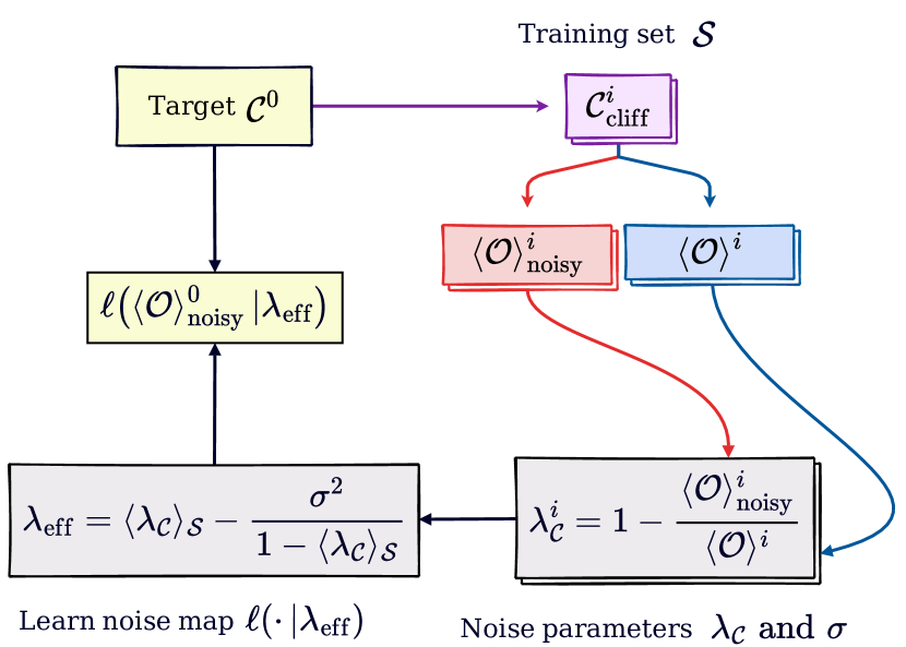
Figure 3: Importance Clifford Sampling is a learning based error mitigation algorithm that uses a set of Clifford circuits to learn a noise map to mitigate the expected value of a given observable.

When $\mathcal{O}$ is a Pauli string, the noise-free expected values will concentrate on $-1$, $0$, $1$ [64]. Furthermore, as discussed in [17], not all the Clifford circuits are error sensitive. In particular, we only need circuits whose expected values on Pauli’s are $\pm 1$. We refer to these circuits as non-zero circuits for simplicity. Unfortunately, sampling non-zero circuits is exponentially rare when the number of qubits increases, thus a strategy has to be defined to efficiently build a suitable training set. We follow the ICS algorithm [17], in which non-zero circuits are built by adding a layer of Pauli gates to zero circuits. These gates can be merged with the ones following so that the depth does not increase.

The generated set is then used to train a model to learn a mapping between $\langle\mathcal{O}\rangle_{\text{noisy}}$ and $\langle\mathcal{O}\rangle$. The structure of the model $\ell$ can be inspired by considering the action of a global depolarizing channel with depolarizing parameter $\lambda$,

$$\langle\mathcal{O}\rangle_{\text{noisy}}=(1-\lambda)\langle\mathcal{O}\rangle+\frac{\lambda}{d}\operatorname{Tr}(\mathcal{O})\ ,$$ (9)

where $d=2^{n}$ denotes the dimension of the Hilbert space and $0<\lambda<4^{n}/(4^{n}-1)$. Focusing on Pauli strings and allowing $\lambda$ to take any value, we arrive at the phenomenological error model,

$$\langle\mathcal{O}\rangle_{\text{noisy}}^{i}=(1-\lambda_{\mathcal{C}}^{i})\langle\mathcal{O}\rangle^{i}\ ,$$ (10)

from which we can calculate $\lambda_{\mathcal{C}}^{i}$ for each circuit in the training set. This set of depolarizing parameters, characterized by the mean value $\lambda_{0}=\langle\lambda_{\mathcal{C}}\rangle_{\mathcal{S}}$ and standard deviation $\sigma$, allows to define an effective depolarizing parameter for mitigating the initial circuit,

$$\lambda_{\text{eff}}=\lambda_{0}-\frac{\sigma^{2}}{1-\lambda_{0}}\ .$$ (11)

This translates into the noise map,

$$\ell\bigl{(}\langle O\rangle|\lambda_{\text{eff}}\bigr{)}=\frac{(1-\lambda_{0})}{(1-\lambda_{0})^{2}+\sigma^{2}}\langle O\rangle_{\rm noisy}\ .$$ (12)

The average depolarizing rate $\lambda_{0}$ scales proportionally with the number of gates, while the standard deviation $\sigma$ is proportional to its square root [17]. This implies that the model performs better as the circuit depth increases.

The noise map (12) effectively handles symmetric readout noise, but fails with asymmetric noise. For these situations, we employ Bayesian Iterative Unfolding (BIU) [66] to mitigate measurement errors in advance.

A schematic representation of the described algorithm is reported in Fig. 3.

III The RTQEM algorithm

We implement an Adam optimization mitigating both gradients and predictions following the procedure presented in Sec. II.1.1.

In a real quantum computer, small fluctuations of the conditions over time, such as temperature, may result in a change of the shape of the noise sufficient to deteriorate results. Therefore, we compute a metric

$$D(z,\ell(z))=|z-\ell(z)|$$ (13)

at each optimization iteration, which quantifies the distance between a target noiseless expected value $z$ and the mitigated estimation $\ell(z)$. These expected values are calculated over a single non-zero test circuit to maximize the bias. If an arbitrary set threshold value $\varepsilon_{\ell}$ is exceeded, the noise map is relearned from scratch. A schematic representation of the proposed procedure is reported in Alg. 1.

Set $N_{\rm update},N_{\rm epoch},k=0$ ;

Initialize VQC parameters $\bm{\theta}_{k}$, noise map $\ell$ ;

Define target noiseless expectation value $z$ ;

Define metric $D(z,\ell(z))$ to check $\ell$ reliability;

for $k<N_{\rm epochs}$ do

       if $D(z,\ell(z))>\varepsilon_{\ell}$ then

             learn $\ell_{k}$;

             $\ell\leftarrow\ell_{k}$;

            

       end if

      compute $\ell({\bm{y}}_{\rm est})$;

       calculate $J\bigl{[}\ell(\bm{y}_{\rm est}),\bm{y}_{\rm meas}\bigr{]}$;

       for $p\in\bm{\theta_{k}}$ do

             compute $\ell(\partial_{p}J)$ via PSR;

            

       end for

      $\bm{\theta}_{k+1}$ $\leftarrow$ Adam$(\bm{\theta}_{k})$;

end for

Algorithm 1 RTQEM

IV Validation

We propose two different experiments to test the RTQEM algorithm introduced above. Firstly, in Sec. IV.1, we simulate the training of a VQC on both a single and a multi-qubit noisy device. Whereas, in Sec. IV.2, the same procedure is deployed on a superconducting single-qubit chip. The programs to reproduce such simulations can be found at [67].

IV.1 Simulation

In this section, we benchmark different levels of error mitigation by conducting both noisy and noiseless classical simulations with $N_{\rm shots}=10000$ shots as outlined in Tab. 1. The VQC shown in Fig. 2 is used as ansatz and the noise is described by the noise model presented in Section II. We first consider a static-noise scenario in Section IV.1.1, while in Section IV.1.2 we let the noise vary over time.

Training	Noise	RTQEM	QEM at the end
Noiseless	2613	2613	2613
Noisy	1F5F8	2613	2613
fQEM	1F5F8	2613	1F5F8
RTQEM	1F5F8	1F5F8	1F5F8

Table 1: Summary of the tested simulation configurations.

IV.1.1 Static-noise scenario

The following simulations are performed using a static local Pauli noise model where we set the following noise parameters $q_{x}=0.007$, $q_{y}=0.003$, $q_{z}=0.002$ and $q_{M}=0.005$.

We first consider a one-dimensional target, namely, the $u$-quark Parton Distribution Function (PDF) for a fixed energy scale $Q_{0}$ with varying momentum fraction $x$ sampled from the interval $[0,1]$. A logarithmic sampling is used to improve the resolution of the $x\sim(0,0.1)$ range where the shape of the function is more rugged. The corresponding PDF values are provided by the NNPDF4.0 grid [68]. We address this first target by constructing a four-layer single-qubit circuit, following the ansatz depicted in Fig. 2. The results, shown in Fig. 4, illustrate that the RTQEM approach enables the training to converge to the correct solution.

To avoid the u-quark PDF comfortably resting below the bound (7) and thereby disguising the effect of the NIBP, we opted to expand it to cover the range $[0,1]$. One might wonder whether a similar, but opposite, trick could be employed in case that the bound intercepts the target function. Therefore, compressing the function to make it lie below the bound and avoid any sort of limitations on the predictions. While this is a perfectly viable method in theory, it is essentially pointless in practice. The compression of the function, indeed, will also increase the precision needed to resolve it, which translates in a larger number of shots required by each prediction [16].

The noisy simulation is clearly limited by loss concentration (7), which caps the predictions at around $y\simeq 0.85$. This limit is also noticeable in Fig. 4, where the loss value cannot decrease below the threshold with unmitigated training. Attempting to correct the predictions post-training (f-QEM) allows access to the region above the bound, but does not enhance the fit. This is expected, as the noise shifts the position of the minima of the loss function making it impossible to retrieve the true minimum with a final rescaling pass alone. However, by gradually cleaning up the loss function landscape during the training, the correct minimum is recovered, and the fit converges to the target function.

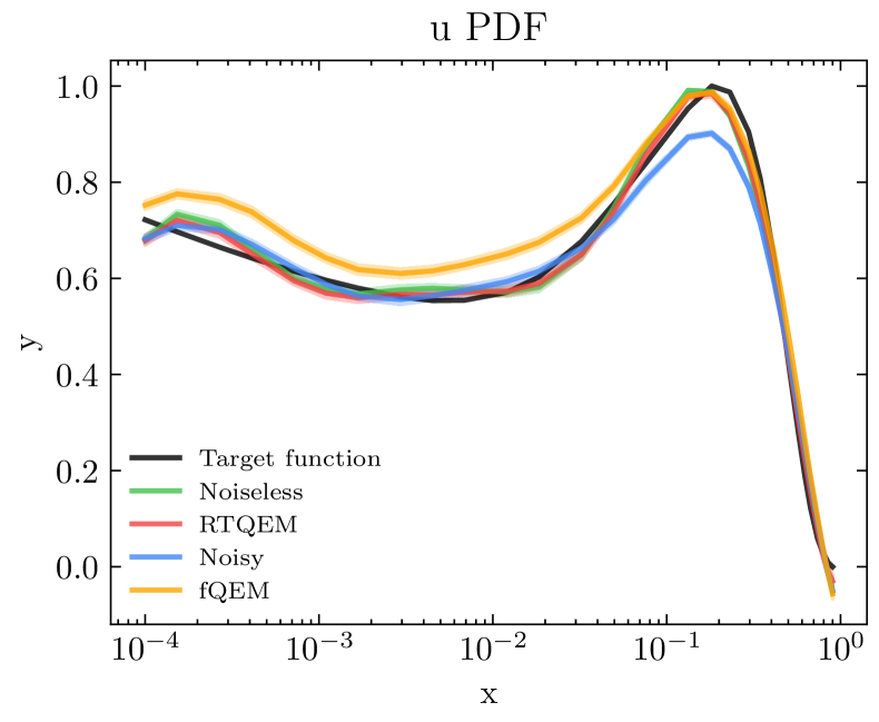
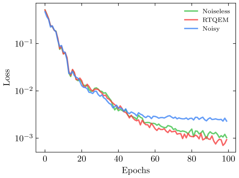
Figure 4: Estimates of $u$-quark PDF associated to $N_{\rm data}=50$ momentum fraction values sampled logarithmically in $[0,1]$. The NNPDF4.0 measures (black line) are compared with results obtained through noiseless simulation (green line), noisy simulation (blue line), noisy simulation with mitigation applied to the final predictions (yellow line) and real-time mitigated noisy simulation (red line). The effective depolarizing parameter $\lambda_{\text{eff}}$ is $0.09\pm 0.01$. The final predictions are computed averaging on $N_{\rm runs}=100$ predictions calculated for each of the $N_{\rm data}$ points. The confidence intervals are obtained using one standard deviation from the mean. The bottom plot shows the loss function history for each training scenario.

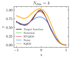
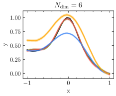
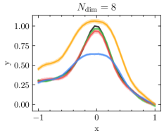
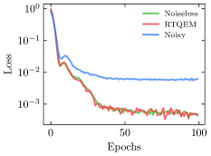
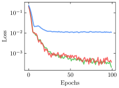
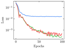
Figure 5: Predictions for the multidimensional function $f_{\rm ndim}$ with $N_{\rm dim}=4,6,8$ from left to right. The exact predictions (black line) are compared with results obtained through noiseless simulation (green line), noisy simulation (blue line), noisy simulation with mitigation applied to the final predictions (yellow line) and real-time mitigated noisy simulation (red line). The effective depolarizing parameters $\lambda_{\text{eff}}$ are $0.22\pm 0.02$ ($N_{\rm dim}=4$), $0.31\pm 0.03$ ($N_{\rm dim}=6$) and $0.41\pm 0.02$ ($N_{\rm dim}=8$). The final predictions are computed averaging on $N_{\rm runs}=20$ predictions calculated for each of the $N_{\rm data}=30$ points. The confidence intervals are obtained using one standard deviation from the mean. The bottom plot shows the loss function history for each training scenario.

To better understand how the algorithm scales with the number of qubits we study the problem of fitting a multi-dimensional function. In particular, we consider

$$f_{\rm ndim}(\bm{x};\bm{\beta})=\sum_{i=1}^{N_{\rm dim}}\bigl{[}\cos{(\beta_{i}x_{i})^{i}}+(-1)^{i-1}\beta_{i}x_{i}\bigr{]},$$ (14)

where both data $\bm{x}$ and parameters $\bm{\beta}$ have dimension $N_{\rm dim}$ and the index $i$ runs over the problem dimensions. In particular, the model parameters $\bm{\beta}$ are defined as equidistant point in the range $[0.5,2.5]$, and they are kept fixed during the optimization. The target $f_{\rm ndim}$ is rescaled in order to occupy the range $[0,1]$. We consider $N_{\rm data}$ values for each $x_{i}\in\bm{x}$ homogeneously distributed in the range $[0,1]$. The ansatz is the $N_{\rm dim}$-qubit circuit of Fig. 2 with three layers.

As the dimensionality of the problem increases, and consequently, the number of qubits, the noise-induced bound is lower, hindering the description of the function in a region of its domain. By applying the RTQEM algorithm, we manage to achieve lower values of the loss function, thereby improving the quality of the fit (see Fig. 5). These results are confirmed by computing the Mean Squared Error (MSE) metric,

$$\text{MSE}=\frac{1}{N_{\rm data}}\sum_{j=1}^{N_{\rm data}}(\bar{y}_{\rm est}^{j}-y_{\rm meas}^{j})^{2}\ ,$$ (15)

where $\bar{y}_{\rm est}^{j}$ is the average estimate of $f(\bm{x}^{j})$ over $N_{\rm runs}$. The MSE associated to each fit is shown in Tab. 2.

Target	$\text{MSE}_{\rm noiseless}$	$\text{MSE}_{\rm noisy}$	$\text{MSE}_{\rm fqem}$	$\text{MSE}_{\rm rtqem}$
$u$ PDF	$0.008$	$0.018$	$0.023$	$0.008$
$\cos 4$d	$0.003$	$0.043$	$0.140$	$0.003$
$\cos 6$d	$0.002$	$0.083$	$0.214$	$0.002$
$\cos 8$d	$0.001$	$0.118$	$0.360$	$0.004$

Table 2: Mean squared error distances between the target functions and the VQC fitting model trained under the different conditions of Tab. 1.

Regarding the gradients, it is important to note that there are no significant differences between the raw gradients and the exact gradients (see Appendix A). This means that we are in a regime where the loss concentration is not severe, and there is still room for error mitigation to improve trainability by mitigating other unwanted effects in the landscape due to the noise.

IV.1.2 Evolving-noise scenario

To study the performance of the method with noise evolution, we consider a random change in the Pauli parameters of the noise model in each epoch. In particular, the initial parameters vector $\bm{q}^{0}=(q_{x}^{0},q_{y}^{0},q_{z}^{0})$ is moved in its three-dimensional space following a procedure similar to a Random Walk (RW) on a lattice. Namely, each component $q_{j}$ is evolved from epoch $k$ to epoch $k+1$ as

$$q_{j}^{(k+1)}=q_{j}^{k}+r\delta,$$ (16)

where $r\sim\{-1,+1\}$ and the step length is sampled from a normal distribution $\delta\sim\mathcal{N}(0,\sigma_{\delta})$. We refer to an evolution performing $N$ steps governed by $\sigma_{\delta}$ as $\text{RW}^{N}_{\sigma_{\delta}}$. The readout noise parameter is kept fixed at the value of $q_{M}=0.005$. In this evolving scenario, when the metric (13) exceeds a certain threshold $\varepsilon_{\ell}$, the mitigation parameter $\lambda_{\text{eff}}$ (11) is updated.

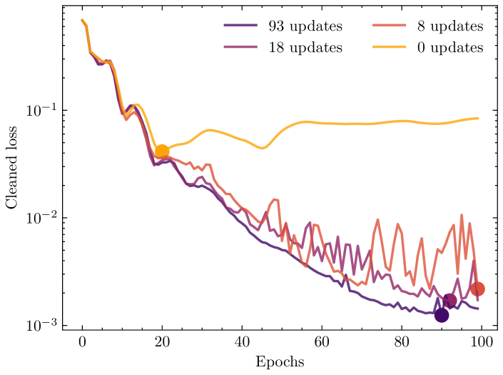
Figure 6: Four RTQEM training simulations sharing the same initial conditions. The initial local Pauli parameters $\bm{q}^{0}=(0.005,0.005,0.005)$ are evolved under a $\text{RW}_{0.002}^{100}$. The readout noise parameter has been kept fixed to $q_{M}=0.005$, four layers are used with $N_{\rm data}=30$ and $\eta=0.05$. For each training simulation a different noise threshold value was used: $\varepsilon_{\ell}=\{0,0.05,0.1,0.2\}$. As a result, $\lambda_{\text{eff}}$ is re-learned $u=\{93,18,8,0\}$ times, respectively. We show the loss function values computed using the training parameters at each iteration but deployed in a noiseless scenario.

To evaluate the effect of relearning the noise on the training process, we track the evolution of the loss function of the $u$-quark PDF for various values of $\varepsilon_{\ell}$, as shown in Fig. 6. We aim for a reduction in the loss function to correspond to a closer approximation to the noise-free parameters. Therefore, we recalculate the loss function values at each iteration using the noisy training parameters, but in a noiseless simulation. As the threshold decreases, the noise map is updated more frequently. It is expected that a lower threshold will enhance the training until it reaches a certain minimum value, characterized by the standard deviation of $\lambda_{\text{eff}}$. Interestingly, even a few updates to the noise map can lead to significantly lower values for the loss function. For instance, the difference between the minimum values of the loss function when updating the noise map 8 times as opposed to 93 times during a training of 100 epochs is $\mathcal{O}\left(10^{-3}\right)$. This suggests that a minor additional classical computational cost can significantly improve the training.

IV.2 Training on hardware

We set up our full-stack gradient descent training on a superconducting device hosted by the Quantum Research Center (QRC) in the Technology Innovation Institute (TII). The high-level algorithm is implemented with Qibo [28, 29, 30, 31] and then translated into pulses and executed on the hardware through the Qibolab [32, 33] framework (see Appendix B). The qubit calibration and characterization have been performed using Qibocal [35, 36]. In particular, we use one qubit of Soprano, a five-qubit chip constructed by QuantWare [69] and controlled using Qblox [70] instruments (see Appendix C). We refer to this device as qw5q.

The $u$-quark PDF for a fixed energy scale $Q_{0}$ is targeted using a four layer single-qubit circuit built following the ansatz presented above. We take $N_{\rm data}=15$ values of the momentum fraction $x$ sampled from the interval $[0,1]$.

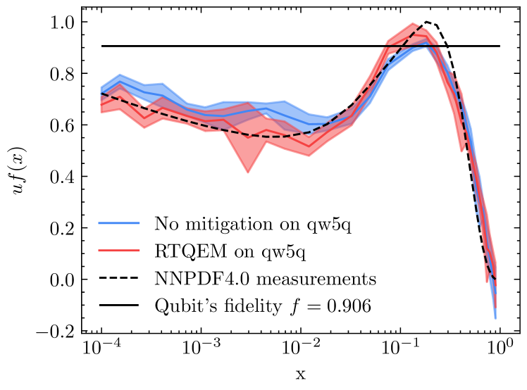
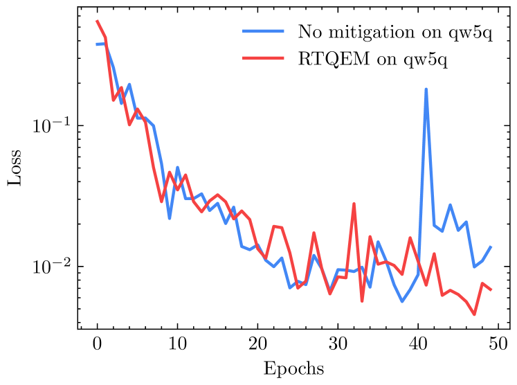
Figure 7: Above, estimates of $N_{\rm target}=30$ values of the $u$-quark PDF obtained by training the best qubit of the qw5q chip. The target values (black dashed line) are compared with our predictions after an unmitigated training (blue line) and a training with RTQEM (red line). The estimations are computed averaging over $N_{\rm runs}=10$ predictions for each $x$ with the trained $\bm{\theta}_{\rm best}$. The same prediction sets allow to calculate the standard deviations of the estimates, which are then used to draw the confidence intervals. Below, loss function history as function of the optimization epochs. The effective depolarizing parameter is $\lambda_{\rm eff}=0.07\pm 0.03$.

An estimate to the bound imposed by the noise is provided by the assignment fidelity of the used qubits, which are collected in dedicated runcards describing the current status of the QRC devices [71]. As with the simulation, we adjust the function to span the range $[0,1]$.

Param	$N_{\rm epochs}$	$N_{\rm shots}$	$N_{\rm train}$	$N_{\rm params}$	$\eta$	NumPy seed
Value	$50$	$500$	$15$	$16$	$0.1$	$1234$

Table 3: Hyper parameters of the gradient descent on qw5q

We perform a gradient descent on the better calibrated qubit of qw5q using the parameters collected in Tab. 3. The training has been performed for both the unmitigated and the RTQEM approaches. After training, we repeat $N_{\rm runs}=10$ times the predictions for each one of $N_{\rm target}=30$ target values of $x$ sampled logarithmically from $[0,1]$. The final estimate to the average prediction and its corresponding standard deviation are computed out of the $N_{\rm runs}$ repetitions.

The RTQEM process leads to better compatibility overall and, in particular, is able to overcome the bound set by the noise represented as a black horizontal line, as shown in Fig. 7. Indeed, the mitigated fit leads to a smaller MSE compared to the unmitigated one, as reported in Tab. 4. This proves that the RTQEM procedure gives access to regions which are naturally forbidden to the raw training.

As a second test, we push forward the RTQEM training by performing a longer optimization. We use the same hyper-parameters of Tab. 3 but set $N_{\rm epochs}=100$, with the aim of finding more reliable parameters. We repeat the optimization twice, adopting the same initial conditions but changing the device. We use the aforementioned qw5q and a different five-qubit chip constructed by IQM [72] and controlled using Zurich [73] Instruments (see Appendix C). We refer to this device as iqm5q.

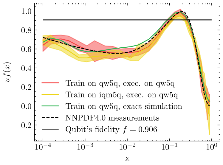
Figure 8: Estimates of $N_{\rm target}=30$ values of the $u$-quark PDF obtained by training the better calibrated qubits of qw5q and iqm5q, respectively with assignment fidelities $f_{\rm qw5q}=0.906$ and $f_{\rm iqm5q}=0.967$. The target values (black dashed line) are compared with our RTQEM predictions obtained by training for $N_{\rm epochs}=100$ on both qw5q (red line) and iqm5q (yellow line). We also show the predictions computed deploying in exact simulation mode the best parameters obtained through RTQEM training on qw5q (green line). The final average and standard deviation of the predictions are computed out of $N_{\rm runs}=20$ repetition for each $x$ using the parameters $\bm{\theta}_{\rm best}$ learned during training. In particular, the $1\sigma$ confidence intervals are shown in the plot. The effective depolarizing parameter is $\lambda_{\rm eff}=0.08\pm 0.02$.

Training	Predictions	Config.	$N_{\rm epochs}$	MSE
qw5q	qw5q	Noisy	$50$	$0.0055$
qw5q	qw5q	RTQEM	$50$	$0.0042$
qw5q	qw5q	RTQEM	$100$	$0.0013$
iqm5q	qw5q	RTQEM	$100$	$0.0037$
qw5q	sim	RTQEM	$100$	$0.0016$

Table 4: MSE values for the models trained on the hardware. The column “Training” indicates the device where the training took place, whereas the column “Predictions” specifies the device where the model is deployed for testing.

If the parameters obtained through RTQEM procedure are noise independent, we expect them to be generally valid. Namely, the optimal parameters obtained for one device, should lead to a valid fit when deployed to a different one. This is illustrated in Fig. 8, where we report the results obtained by training individually on qw5q and on iqm5q with the same initial conditions, and then deploying the two sets of obtained parameters solely on qw5q. The plotted estimates are computed by averaging on $N_{\rm runs}=20$ repeated predictions.

Finally, to further verify that the obtained parameters are indeed noise-independent, we deploy the model obtained by training on qw5q via RTQEM on an exact simulator (green line in Fig. 8).

We calculate the MSE value for each described experiment following 15. All the results are collected in Tab. 4, and confirm that the RTQEM training leads to noise-indipendent modelization.

V Conclusion

In this paper, we introduced a new Real-Time Quantum Error Mitigation (RTQEM) routine designed to enhance the training process of Variational Quantum Algorithms. We employed the Importance Clifford Sampling method at each learning step to mitigate noise in both the gradients of the loss function and the predictions. The RTQEM algorithm effectively reduces loss corruption without exacerbating loss concentration, thereby guiding the optimizer towards lower local minima of the loss function. We evaluated the RTQEM procedure using superconducting qubits and found that it improved the fit’s consistency by surpassing the limitations imposed by the hardware’s noise.

Our results demonstrate that the proposed algorithm effectively trains Variational Quantum Circuit (VQC) models in noisy environments. Specifically, if the system’s noise remains constant or changes slowly, the noise map requires only a few updates during training, keeping the computational cost on par with the unmitigated training process.

Notably, by mitigating noise during training, we can derive parameters that closely approximate those of a noise-free environment. This adaptability allows us to deploy these parameters on a different device, even if it is subject to different noise. This capability paves the way for the potential integration of federated learning with quantum processors.

The extension of this approach to other QML pipelines that use expected values as predictors, as well as to other QEM methods, presents an intriguing avenue for future research. For instance, it can be applied to VQC models for supervised, unsupervised, and reinforcement learning scenarios in noisy environments.

Appendix A Gradients evolution

During the VQC training, the noisy gradients are of the same magnitude as the exact ones, indicating that we are in a regime where exponential concentration is not severe, as shown in Fig. 9.

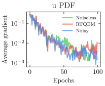
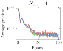
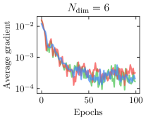
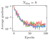
Figure 9: Average gradients as function of the optimization epochs. A noiseless simulation (green lines) is compared with unmitigated noisy simulation (blue lines) and RTQEM (red lines) for $N_{\rm dim}=4,6,8$ from the left to the right plots.

Appendix B Native gates

The native gates of the QRC superconducting quantum processors are $RX(\pm\pi/2)$, $RZ(\theta)$, and $CZ$ gates [71]. They constitute a universal quantum gate set. These gates are compiled into microwave pulses following a specific set of rules [32]. For a circuit to be executable on hardware, it needs to be decomposed into these native gates. For instance, a general single-qubit unitary beaks into a sequence of five native gates,

$$U(\theta,\phi,\lambda)=RZ(\phi)RX(-\pi/2)RZ(\theta)RX(\pi/2)RZ(\lambda)\ .$$ (A1)

Appendix C Qubits’ parameters

Relevant parameters of the qubits utilized in this study are presented in Tab. 5, including:

1. the qubit transition frequency $f_{01}=\omega_{q}/2\pi$ from $\ket{0}$ to $\ket{1}$;

2. the bare resonator frequency $f_{\rm res}=\omega_{\rm res}/2\pi$;

3. the readout frequency $f_{\rm read}$ (coupled resonator frequency);

4. the energy relaxation time $T_{1}$;

5. the dephasing time $T_{2}$;

6. the time $\tau_{g}$ required to execute a single $RX$ gate;

In the same table we also show the assignment fidelity $f=1-[P(1|0)-P(0|1)]/2$, where $P(i|j)$ is a misclassification metric, counting the states prepared as $\ket{j}$ but measured as $\ket{i}$. This value is primarily due to the calibration status of the devices, rather than construction limitations.

Qubit	$f_{01}({\rm GHz})$	$f_{\rm res}({\rm GHz})$	$f_{\rm read}({\rm GHz})$	$T_{1}(\mu\text{s})$	$T_{2}(\mu\text{s})$	$\tau_{g}({\rm ns})$	$f$
qubit 4, iqm5q	$4.0978$	$5.5047$	$5.5150$	$9.891$	$3.700$	$40$	$0.967$
qubit 3, qw5q	$6.7599$	$7.8000$	$7.8028$	$2.776$	$1.139$	$40$	$0.906$

Table 5: Parameters of the iqm5q and qw5q qubits employed in this study.