Enhanced quantum phase synchronization of a laser-driven qubit under non-Markovian dynamics

Abstract

In this paper, we demonstrate transient dynamics of Husimi $Q$-representation to visualize and characterize the phase synchronization behavior of a two-level system (qubit) driven by a laser field in both the Markov and non-Markov regime. In the Markov regime, phase preference of the qubit goes away in the long time limit, whereas the long-time phase localization persists in the non-Markovian regime. We also plot the maximum of the shifted phase distribution in two different ways: (a) by varying the detuning and laser drive strength, and (b) by varying the system-bath coupling and laser drive strength. Signature of quantum phase synchronization viz the Arnold tongue is demonstrated through the maximal value of the shifted phase distribution. The phase synchronization is observed inside the tongue region while the region outside the tongue is desynchronized. The synchronization regions are determined by various system-environment parameters and the qubit phase synchronization is shown to be enhanced in the non-Markov regime.

I Introduction

Synchronization is a natural phenomenon that occurs in a variety of physical, chemical, and biological systems and has been extensively studied and observed in nature for many years [1, 2, 3, 4, 5]. A well-known example of classical synchronization is the van der Pol oscillator model [4, 5]. For example, if an autonomous oscillating system is coupled to another such system or an external driving force, it can synchronize its frequency and phase to the external system [6]. In the past year ago, the van der Pol model was reformulated in the terms of a quantum system [7, 8], and it was demonstrated that as it is close to the ground state, this correspondence is changed because the discreteness of the energy levels becomes important. Recently, quantum synchronization in low-dimensional systems has been intensively studied [9, 10, 11]. An investigation into the fewest possible energy levels or the smallest possible system [9] that can be carried out synchronization arises. In general, quantum synchronization arises can be classified into forced and mutual synchronization [12, 13]. In the forced synchronization or entrainment, there is a synchronization of a qubit is an additional feature experienced due to the presence of other qubits, or as the driving due to an external field [9, 14, 15] and as well as the investigation of quantum synchronization induced by the environment was carried out in Ref. [16, 17]. In the absence of a driving field, synchronization may emerge as a collective phenomenon as a result of coherent dynamics, which is referred to as mutual synchronization. Mutual synchronization occurs due to the dynamics of qubits coupled to an external environment in Ref. [18, 19], qubits are proposed to be finite levels or the smallest possible system that can be synchronized. However, subsequent research [9] claimed that synchronization cannot occur in dissipative two level systems. Following that, it was demonstrated that synchronization of a qubit to an external signal is possible [20, 21, 22]. Synchronization has been studied in the quantum world [13], where spontaneous synchronization [23, 24, 25, 26] have been investigated in a variety of systems including spins, and harmonic and nonlinear oscillators, modeling platforms ranging from optomechanical systems to trapped ions and superconducting qubits. Synchronization signatures have also recently been reported in experiments [27, 28]. Here the authors [16, 17] explore the relationship between non-Markovianity and two qubit synchronization using a phenomenological Lindblad-type master equation as well as a collision model.

In the present work, we investigate transient phase synchronization for a two-level system (qubit) driven by a semiclassical laser field and simultaneously coupled to a dissipative environment. We discuss the phase synchronization in which the qubit synchronizes under the driving in presence of a Markov or non-Markov environment. The rest of the paper is organized as follows. In Sec. II, we consider a widely studied two-level system (qubit) simultaneously interacting with a dissipative environment while being driven by an external field. The time evolution of the reduced density matrix of the qubit is considered to be two distinct types of dynamics depending on $\left(1\right)$ the reservoir correlation time is being very small compared to the relaxation time of the qubit and the dynamics corresponds to Markovian dynamics. On the other hand, $\left(2\right)$ the reservoir correlation time is of the same order as the system relaxation time and connected with non-Markovian effects [30]. In Sec. III, we demonstrate the transient dynamics of the Husimi $Q$-representation in order to visualize and characterize phase synchronization behavior in both the Markov and non-Markov regimes. In Sec. IV, we consider a measure of synchronization, called shifted phase distribution, and show its dynamics as a function of phase and detuning in the Markov and non-Markovian regimes. We also plot the maximum value of the shifted phase distribution in two different ways: (a) by varying the detuning and laser drive strength, and (b) by varying the system-bath coupling and laser drive strength. Signature of quantum phase synchronization viz the Arnold tongue is demonstrated through the maximal value of the shifted phase distribution. Finally, we present our conclusions in Sec. V.

II Model of laser-driven qubit and time evolution

We consider a single two-level system (TLS) driven by a semiclassical laser field of strength $\epsilon$ with driving frequency $\omega_{L}$, which is simultaneously coupled to a dissipative environment. In the rotating-wave approximation (RWA), the total Hamiltonian of the system plus environment and the external driving is given by

$$H=\frac{\hbar}{2}\omega_{0}{\sigma}_{z}+\sum_{k}\hbar\left(g_{k}{\sigma}_{+}b_{k}+g_{k}^{\dagger}{\sigma}_{-}b_{k}^{\dagger}\right)+\sum_{k}\hbar\omega_{k}b_{k}^{\dagger}b_{k}+i\hbar\frac{\epsilon}{4}\left(e^{i\omega_{L}t}{\sigma}_{-}+e^{-i\omega_{L}t}{\sigma}_{+}\right),$$ (1)

where the qubit has the transition frequency $\omega_{0}$ between the ground state $\left|0\right\rangle$ and excited state $\left|1\right\rangle$. The system Hamiltonian $\frac{\hbar}{2}\omega_{0}{\sigma}_{z}$ is expressed in term of the spin rasing and lowering operators ${\sigma}_{+}=\left|1\right\rangle\left\langle 0\right|$ and ${\sigma}_{-}=\left|0\right\rangle\left\langle 1\right|$. A dissipative environment’s Hamiltonian is described by a collection of infinite bosonic modes with the bosonic creation and annihilation operators denoted by $b_{k}^{\dagger}$ and $b_{k}$, respectively, and $g_{k}$ is the coupling strength between the system and the $k$th mode of the environment with frequency $\omega_{k}$. Through the unitary transformation, $U(t)=e^{\frac{i}{2}{\sigma}_{z}\omega_{L}t}$, we go to a frame rotating at the laser driving frequency. The total Hamiltonian under this transformation becomes

$$H=H_{\text{TLS}}+H_{\text{SR}}+H_{\text{R}}=\frac{\hbar}{2}\Delta{\sigma}_{z}+\frac{\hbar}{2}\epsilon{\sigma}_{x}+\sum_{k}\hbar\left(g_{k}{\sigma}_{+}b_{k}e^{i\omega_{L}t}+g_{k}^{\ast}{\sigma}_{-}b_{k}^{\dagger}e^{-i\omega_{L}t}\right)+\sum_{k}\hbar\omega_{k}b_{k}^{\dagger}b_{k},$$ (2)

where $\Delta=\omega_{0}-\omega_{L}$ represents the detuning with the laser driving. The two-level system Hamiltonian can precisely be diagonalized as

$$H_{\text{TLS}}=\frac{\hbar}{2}\Delta{\sigma}_{z}+\frac{\hbar}{2}\epsilon{\sigma}_{x}=\frac{\hbar}{2}\delta{\bar{\sigma}}_{z},$$ (3)

where we use basis transformation $|{\bar{1}}\rangle=\cos\frac{\theta}{2}\left|1\right\rangle+\sin\frac{\theta}{2}\left|0\right\rangle$, and $|{\bar{0}}\rangle=-\sin\frac{\theta}{2}\left|1\right\rangle+\cos\frac{\theta}{2}\left|0\right\rangle$, and we choose $\tan$ $\theta=\frac{\epsilon}{\Delta}$ and $\delta=\sqrt{\Delta^{2}+\epsilon^{2}}$. We define the spin operators in the new basis as ${\bar{\sigma}}_{+}=\left|{\bar{1}}\right\rangle\left\langle{\bar{0}}\right|$, ${\bar{\sigma}}_{-}=\left|{\bar{0}}\right\rangle\left\langle{\bar{1}}\right|$, and ${\bar{\sigma}}_{z}=\left|{\bar{1}}\right\rangle\left\langle{\bar{1}}\right|-\left|{\bar{0}}\right\rangle\left\langle{\bar{0}}\right|$. In the interaction picture, the interaction Hamitonian is given by

$$H_{\text{SR}}(t)=\sum_{k}\hbar g_{k}\left[P_{\text{0}}{\bar{\sigma}}_{z}+P_{+}{\bar{\sigma}}_{+}+P_{-}{\bar{\sigma}}_{-}\right]b_{k}~{}e^{i(\omega_{L}-\omega_{k})t}+\text{H.c.},$$ (4)

where $P_{\text{0}}=\frac{\epsilon}{2\delta},$ $P_{+}=\frac{\Delta+\delta}{2\delta},$ and $P_{-}=\frac{\Delta-\delta}{2\delta}$. The interaction Hamiltonian can finally be expressed as

$$H_{\text{SR}}\left(t\right)=S(t)B\left(t\right)+\text{H.c.},~{}~{}\mbox{where}$$ (5)

$$B\left(t\right)=\sum_{k}g_{k}b_{k}e^{-i\omega_{k}t}~{}~{}\mbox{is the reservoir operator and}$$ (6)

$$S(t)=\left(P_{\text{0}}{\bar{\sigma}}_{z}+P_{+}{\bar{\sigma}}_{+}e^{i\delta t}+P_{-}{\bar{\sigma}}_{-}e^{-i\delta t}\right)e^{i\omega_{L}t}.$$ (7)

There are three distinct jump processes, $P_{\text{0}}$ denotes elastic tunneling through the bath, whereas $P_{+}\left(P_{-}\right)$ denotes inelastic excitation (relaxation) through the bath. For simplicity, we consider factorized initial system-environment state $\rho_{T}\left(0\right)=\rho\left(0\right)\otimes\rho_{E}\left(0\right)$, and $\rho_{E}\left(0\right)$ assumes initial thermal equilibrium state,

$$\rho_{E}\left(0\right)=\exp\left(-\beta H_{\text{R}}\right)/Tr\left[\exp\left(-\beta H_{\text{R}}\right)\right].$$ (8)

Here $\beta=1/k_{B}T$ with $k_{B}$ being the Boltzmann constant and $T$ being the temperature. Then the second-order perturbative master equation in the Schrödinger picture for the two-level system is given by

$$\frac{d\rho}{dt} = -\frac{i\delta}{2}\left[{\sigma}_{z},\rho\right]$$ (9)

$$+\Gamma_{1}\left(t\right)\left[P_{\text{0}}^{2}\left({\sigma}_{z}\rho{\sigma}_{z}-{\sigma}_{z}{\sigma}_{z}\rho\right)+P_{\text{0}}P_{+}\left({\sigma}_{z}\rho{\sigma}_{+}-{\sigma}_{+}{\sigma}_{z}\rho\right)+P_{\text{0}}P_{-}\left({\sigma}_{z}\rho{\sigma}_{-}-{\sigma}_{-}{\sigma}_{z}\rho\right)\right]$$

$$+\Gamma_{2}\left(t\right)\left[P_{-}P_{\text{0}}\left({\sigma}_{+}\rho{\sigma}_{z}-{\sigma}_{z}{\sigma}_{+}\rho\right)+P_{-}P_{+}\left({\sigma}_{+}\rho{\sigma}_{+}-{\sigma}_{+}{\sigma}_{+}\rho\right)+P_{-}^{2}\left({\sigma}_{+}\rho{\sigma}_{-}-{\sigma}_{-}{\sigma}_{+}\rho\right)\right]$$

$$+\Gamma_{3}\left(t\right)\left[P_{+}P_{\text{0}}\left({\sigma}_{-}\rho{\sigma}_{z}-{\sigma}_{z}{\sigma}_{-}\rho\right)+P_{+}^{2}\left({\sigma}_{-}\rho{\sigma}_{+}-{\sigma}_{+}{\sigma}_{-}\rho\right)+P_{+}P_{-}\left({\sigma}_{-}\rho{\sigma}_{-}-{\sigma}_{-}{\sigma}_{-}\rho\right)\right]$$

$$+\Gamma_{4}\left(t\right)\left[P_{\text{0}}^{2}\left({\sigma}_{z}\rho{\sigma}_{z}-\rho{\sigma}_{z}{\sigma}_{z}\right)+P_{\text{0}}P_{+}\left({\sigma}_{-}\rho{\sigma}_{z}-\rho{\sigma}_{z}{\sigma}_{-}\right)+P_{\text{0}}P_{-}\left({\sigma}_{+}\rho{\sigma}_{z}-\rho{\sigma}_{z}{\sigma}_{+}\right)\right]$$

$$+\Gamma_{5}\left(t\right)\left[P_{\text{0}}P_{-}\left({\sigma}_{z}\rho{\sigma}_{-}-\rho{\sigma}_{-}{\sigma}_{z}\right)+P_{+}P_{-}\left({\sigma}_{-}\rho{\sigma}_{-}-\rho{\sigma}_{-}{\sigma}_{-}\right)+P_{-}^{2}\left({\sigma}_{+}\rho{\sigma}_{-}-\rho{\sigma}_{-}{\sigma}_{+}\right)\right]$$

$$+\Gamma_{6}\left(t\right)\left[P_{\text{0}}P_{+}\left({\sigma}_{z}\rho{\sigma}_{+}-\rho{\sigma}_{+}{\sigma}_{z}\right)+P_{-}P_{+}\left({\sigma}_{+}\rho{\sigma}_{+}-\rho{\sigma}_{+}{\sigma}_{+}\right)+P_{+}^{2}\left({\sigma}_{-}\rho{\sigma}_{+}-\rho{\sigma}_{+}{\sigma}_{-}\right)\right],$$

where we have omitted the bars from spin operators, it is implicit that the Pauli spin operators are now in the new basis. The time dependent coefficients in the master equation are denoted by

$$\Gamma_{1}\left(t\right) = \int_{0}^{t}d\tau\int_{0}^{\infty}d\omega J\left(\omega\right)e^{-i\left(\omega-\omega_{L}\right)\left(t-\tau\right)},$$ (10)

$$\Gamma_{2}\left(t\right) = \int_{0}^{t}d\tau\int_{0}^{\infty}d\omega J\left(\omega\right)e^{-i\left(\omega-\omega_{L}+\delta\right)\left(t-\tau\right)},$$ (11)

$$\Gamma_{3}\left(t\right) = \int_{0}^{t}d\tau\int_{0}^{\infty}d\omega J\left(\omega\right)e^{-i\left(\omega-\omega_{L}-\delta\right)\left(t-\tau\right)},$$ (12)

$$\Gamma_{4}\left(t\right) = \int_{0}^{t}d\tau\int_{0}^{\infty}d\omega J\left(\omega\right)e^{i\left(\omega-\omega_{L}\right)\left(t-\tau\right)},$$ (13)

$$\Gamma_{5}\left(t\right) = \int_{0}^{t}d\tau\int_{0}^{\infty}d\omega J\left(\omega\right)e^{i\left(\omega-\omega_{L}+\delta\right)\left(t-\tau\right)},$$ (14)

$$\Gamma_{6}\left(t\right) = \int_{0}^{t}d\tau\int_{0}^{\infty}d\omega J\left(\omega\right)e^{i\left(\omega-\omega_{L}-\delta\right)\left(t-\tau\right)}.$$ (15)

The master equation (9) is a convolutionless and time-local differential equation. The time-dependent coefficients and $\Gamma_{1}\left(t\right)$, $\Gamma_{2}\left(t\right)$, $\Gamma_{3}\left(t\right)$, $\Gamma_{4}\left(t\right)$, $\Gamma_{5}\left(t\right)$, and $\Gamma_{6}\left(t\right)$ account for the memory effect of the non-Markovian environment. To characterize the structured environment and calculate these time-dependent coefficients in equations (10)-(15), we must consider the spectral density to characterize the structured environment. In our case, we will look at an Ohmic spectral density. The time-dependent correlation functions fully characterize the non-Markovian memory effect given the spectral density $J\left(\omega\right)$. Here we consider an Ohmic spectral density [30]

$$J\left(\omega\right)=\gamma\omega\exp\left(-\omega/\lambda\right),$$ (16)

The time-dependent coefficients (10)–(15) appearing in the master equation contain the non-Markovian characteristics of the open quantum system. Here $\gamma$ is the coupling strength between the system and dissipative bath and is measured in units of $\gamma_{0}$ which is a fixed frequency, closely related to the relaxation time of the qubit. In this paper, we have taken $\gamma=0.1\gamma_{0}$ for all results where coupling strength $\gamma$ is fixed. The parameter $\lambda$ is the cutoff frequency of the bath spectrum. We see two distinct types of qubit dynamics based on the value of the system-environment parameters. For $\lambda>2\gamma$, the reservoir correlation time is very short compared to the relaxation time of the qubit and the dynamics is Markovian. When $\lambda<2\gamma$, the reservoir correlation time is comparable to the relaxation time of the qubit and we observe non-Markovian effects. In the Markov regime, we consider a value of $\lambda=5\gamma_{0}$, and in the non-Markov regime $\lambda=0.01\gamma_{0}$. We investigate the qubit phase synchronization for two different values of the detuning, $\Delta=0$ and $\Delta=\gamma_{0}$ respectively.

III Husimi $Q$-function

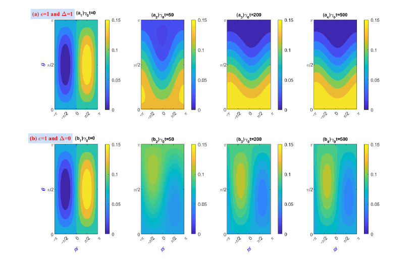
Figure 1: Temporal evolution of the Husimi $Q$-function of a single qubit coupled to a Makovian dissipative bath and under an external driving is shown in the plot for (a) $\epsilon=1$ and $\Delta=1$ (b) $\epsilon=1$ and $\Delta=0$. We have taken the spectral width $\lambda=5\gamma_{0}$ with four different evolution times. The system-environment coupling strength is fixed at $\gamma=0.1\gamma_{0}$.

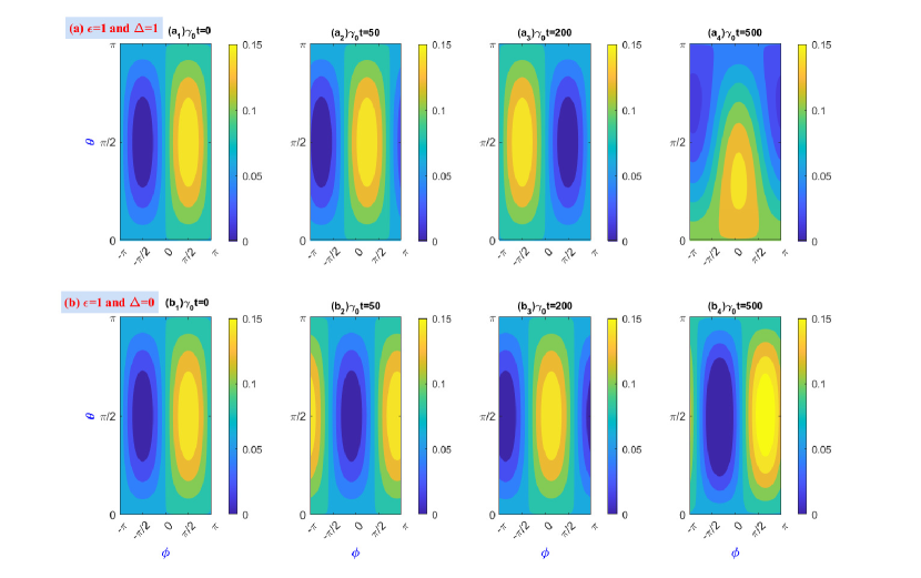
Figure 2: Temporal evolution of the Husimi $Q$-function of a single qubit coupled to a non-Makovian dissipative bath and under an external driving is shown in the plot for (a) $\epsilon=1$ and $\Delta=1$ (b) $\epsilon=1$ and $\Delta=0$. We have taken the spectral width $\lambda=0.01\gamma_{0}$ with four different evolution times. The system-environment coupling strength is taken as $\gamma=0.1\gamma_{0}$.

We use the Husimi $Q$ representation adapted for TLS to visualize and characterize the system’s phase synchronization behavior [29]. The Husimi $Q$-function, a quasiprobability distribution that allows us to represent the phase space of the TLS defined as

$$Q\left(\theta,\phi,t\right)=\frac{1}{2\pi}\left\langle\theta,\phi\right|\rho\left(t\right)\left|\theta,\phi\right\rangle,$$ (17)

where $|\theta,\phi\rangle$ are spin-coherent states, which in the case of a two-level system are the eigenstates of the spin operator $\sigma_{n}=\mathbf{\hat{n}}\cdot\hat{\sigma}$ along the unit vector $\mathbf{\hat{n}}$ with polar coordinates $\theta$ and $\phi$. The states $\left|\theta,\phi\right\rangle$$=\cos\left(\theta/2\right)\left|1\right\rangle+\sin\left(\theta/2\right)e^{i\phi}\left|0\right\rangle$ represents a point on the surface of a Bloch sphere. The basis vectors $\left|0\right\rangle$, and $\left|1\right\rangle$ are the eigenstates of the spin operator $\sigma_{z}$. Once the temporal evolution of reduced density matrix are determined from Eq. (9), it is easy to obtain the time dynamics of $Q$-distribution as a function $\theta$, $\phi$ and $t$ as follows

$$Q\left(\theta,\phi,t\right)=\frac{1}{2\pi}\left[\begin{array}[]{c}\cos^{2}\left(\theta/2\right)\rho_{11}\left(t\right)+\cos\left(\theta/2\right)\sin\left(\theta/2\right)e^{i\phi}\rho_{10}\left(t\right)\\ +\cos\left(\theta/2\right)\sin\left(\theta/2\right)e^{-i\phi}\rho_{01}\left(t\right)+\sin^{2}\left(\theta/2\right)\rho_{00}\left(t\right)\end{array}\right].$$ (18)

The $Q$-function gives the weights of different pure states on the Bloch sphere, contributing to the density matrices at different instants of time.

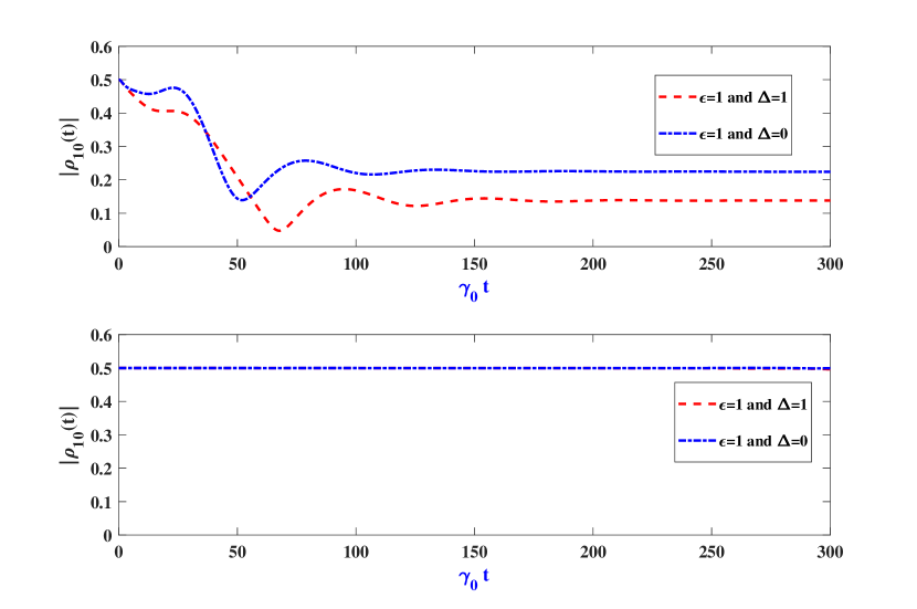
Figure 3: The plot of the off-diagonal element $\left|\rho_{10}\left(t\right)\right|$ as a function of time is given for (a) Markov and (b) non-Markovian evolution. The system-environment coupling strength is taken as $\gamma=0.1\gamma_{0}$.

Figures 1 and 2 show the time-dependent transient dynamics of the $Q\left(\theta,\phi,t\right)$ for Markov and non-Markovian evolution for the initial state $\left|+\right\rangle=\left(\left|0\right\rangle+\left|1\right\rangle\right)/\sqrt{2}$ respectively. The Husimi $Q$-function is shown in Fig. 1 in the Markov regime ($\lambda=5\gamma_{0}$) for two different values of the detuning (a) $\Delta=1$ and (b) $\Delta=0$. We have considered a driving field strength $\epsilon=1$ For $\Delta=1$, we see that $Q$-function is maximum initially at around $\phi=\pi/2$, this phase preference gradually diminishes as the system evolves in time. The $Q$-function becomes uniformly distributed in the long time limit and eventually the phase preference is completely wiped out. According to Fig. 1(b), for zero detuning $\Delta=0$, we see phase preference survives for longer time, say for example, $\gamma_{0}t=500$, where the localized peak of the Husimi $Q$-function has shifted towards $\phi=-\pi/2$. In Fig. 2, we investigate the phase preference in the non-Markovian regime ($\lambda=0.01\gamma_{0}$) for the single qubit system with driving field strength $\epsilon=1$ at two different values of the detuning (a) $\Delta=1$ and (b) $\Delta=0$. Fig. 2 depicts a series of plots displaying the evolution of the localized peak of the Husimi $Q$-function at different times. In Fig. 2, we can see that for non-Markovian evolution phase synchronization persists at different times. The qubit is phase locked in the sense that the $Q$ distribution is mostly contributed from a specific $\phi$ region.

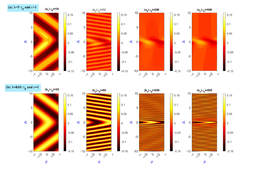
Figure 4: The contour plot of the phase shift distribution $S\left(\phi,t\right)$ as a function of $\Delta$ and $\phi$ for different evolution times $\gamma_{0}t$ is shown with (a) $\epsilon=1$ in Markov case ($\lambda=5\gamma_{0}$) and (b) $\epsilon=1$ in non-Markovian case ($\lambda=0.01\gamma_{0}$). The system-environment coupling strength is taken as $\gamma=0.1\gamma_{0}$.

In Fig. 3, we plot $\left|\rho_{10}\left(t\right)\right|$ as a function of $\gamma t$ for both Markovian and non-Markovian evolution. Our results in Fig. 3(a) show that the phase localization is significantly degraded in the Markov limit for $\epsilon=1$ regardless of $\Delta=1$ or $\Delta=0$ because the phase informative off-diagonal elements are decreasing considerably. Our results in Fig. 3(b) show that synchronization survives in the non-Markov limit for $\epsilon=1$ and $\Delta=1$ due to long lasting off-diagonal elements. The presence of off-diagonal elements (coherences) in the steady state causes phase localization and, as a result, quantum phase synchronization. In Fig. 3(b), when there is a finite detuning in the non-Markov regime, the two level systems exhibit phase synchronization due to information backflow from the external environment. Thus, our findings show that phase localization and, as a result, quantum phase synchronization in the non-Markovian limit is due to long lasting coherence. The synchronization aspects discussed in Ref. [16, 17] are quite different in their origin and features; there are two quantum systems, one of which is influenced by an external bath, which synchronizes the two qubits. The authors refer to it as spontaneous mutual synchronization and discover that information backflow causes the synchronization to be delayed. The origins and characteristics of these two types of synchronizations are quite different [13].

IV Synchronization measure and Arnold’s tongue

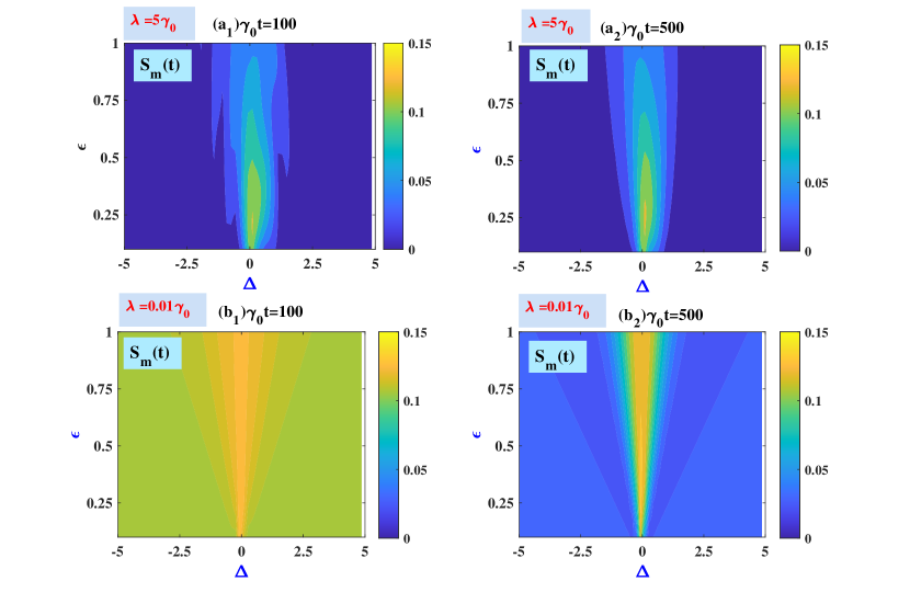
Figure 5: Contour plot of the maximal value of the shifted phase distribution $S_{m}\left(t\right)$ as a function of $\Delta$ and $\epsilon$ in the Markovian regime ($\lambda=5\gamma_{0}$) for two evolution times (a₁) $\gamma_{0}t=100$ and (a₂) $\gamma_{0}t=500$. On the other hand, $S_{m}\left(t\right)$ as a function of $\Delta$ and $\epsilon$ is shown in the non-Markovian regime ($\lambda=0.01\gamma_{0}$) with varying evolution times (b₁) $\gamma_{0}t=100$ and (b₂) $\gamma_{0}t=500$. The system-environment coupling strength is taken as $\gamma=0.1\gamma_{0}$.

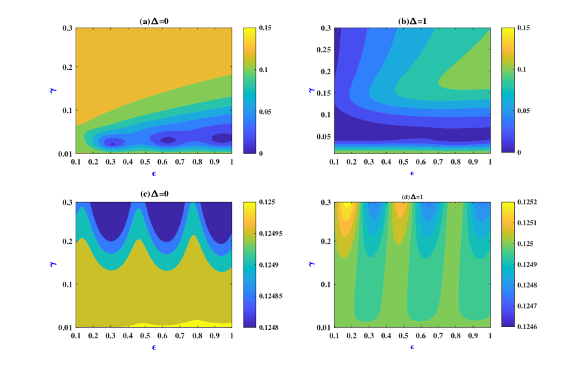
Figure 6: 3D contour plot of $S_{m}(t)$ as a function of $\epsilon$ and $\gamma$ is shown in the Markovian regime ($\lambda=5\gamma_{0}$) for (a) $\Delta=0$ and (b) $\Delta=1$. Next, $S_{m}\left(t\right)$ as a function of $\epsilon$ and $\gamma$ is shown in the non-Markovian regime ($\lambda=0.01\gamma_{0}$) for (c) $\Delta=0$ and (d) $\Delta=1$. The time evolution is fixed at $\gamma_{0}t=500$.

Using the Husimi $Q$-function, a phase-space quasi probability distribution, we investigate phase synchronization for a two-level quantum system. Synchronization in a qubit system is characterised by the Husimi $Q$-function. Furthermore, we use another measure of synchronization, namely, shifted phase distribution for the two-level system [26, 28]. The phase distribution $P(\phi,\rho)$ for a given state is obtained by integrating the $Q$-function over the angular variable ‘$\theta$’. As a result, the synchronization of the qubit system can be measured using the shifted phase distribution following the work done in refs. [23, 24, 25, 26].

$$S\left(\phi,t\right)=\int_{0}^{\pi}Q\left(\theta,\phi,t\right)\sin\theta d\theta-\frac{1}{2\pi}.$$ (19)

This function is zero if and only if the system has no phase preference, implying that phase synchronization is not present. By evaluating the integral over the angular variable $\theta$ we obtain

$$S\left(\phi,t\right)=\frac{1}{8}\left[\rho_{10}\left(t\right)e^{i\phi}+\rho_{01}\left(t\right)e^{-i\phi}\right].$$ (20)

We plot $S\left(\phi,t\right)$ as a function of $\Delta$ and $\phi$ for different evolution times in both the Markov and non-Markov regimes to better understand quantum synchronization. In Fig. 4 (a), we plot the Markov ($\lambda=5\gamma_{0}$) dynamics of $S\left(\phi,t\right)$ at $\epsilon=1$ for the time values $\gamma_{0}t=10$, $\gamma_{0}t=50$, $\gamma_{0}t=200$ and $\gamma_{0}t=500$. There is an interplay between $\Delta$ and $\phi$, quantum phase preferences are displayed through several v-shaped bands. In the Markov regime (see Fig. 4a) the phase localization goes away in the long-time limit, whereas non-Markov dynamics preserves the quantum phase localization in the long time. The non-Markovian ($\lambda=0.01\gamma_{0}$) dynamics of phase synchronization are shown in Fig. 4 (b) through the plots of $S\left(\phi,t\right)$ at $\epsilon=1$ for time values $\gamma_{0}t=10$, $\gamma_{0}t=50$, $\gamma_{0}t=200$ and $\gamma_{0}t=500$ respectively. Figs. 4(b) show that phase synchronization occurs for periodic finite values of detuning in a non-Markovian evolution. For larger values of detuning $\Delta$, we do not see phase localization in the long time for Markov evolution. The maximum of the shifted phase distribution $S_{m}\left(t\right)=\max S\left(\phi,t\right)$ can also be used to characterize phase synchronization. The maximum value of $S\left(\phi,t\right)$ with respect to the phase is found to be $S_{m}\left(t\right)=\frac{1}{4}|\rho_{10}(t)|$. In Fig. 5, we plot $S_{m}\left(t\right)$ as a function of the detuning parameter ($\Delta$) and the laser driving strength ($\epsilon$) for various evolution times in the Markov and non-Markov regimes. In Fig. 5(a), we consider a spectral width of $\lambda=5\gamma_{0}$, while in Fig. 5(b), we consider $\lambda=0.01\gamma_{0}$ and two different times, $\gamma_{0}t=100$ and $\gamma_{0}t=500$. In both plots of Fig. 5(a) and (b), we see the formation of an Arnold tongue. Quantum phase synchronization occurs inside the tongue region, at around $\Delta=0$. The width of the tongue region is enhanced in the non-Markovian region ($\lambda=0.01\gamma_{0}$). This implies that the synchronization region expands with non-Markovian behavior. Quantum synchronization in the system is determined by the parameters detuning ($\Delta$), laser driving strength ($\epsilon$). To get a full picture of synchronization, we plot $S_{m}\left(t\right)$ as a function of the strength of the laser driving ($\epsilon$) and the system-bath coupling strength ($\gamma$) in both the Markov ($\lambda=5\gamma_{0}$) and non-Markov ($\lambda=0.01\gamma_{0}$) regime. In the Markov regime, Figs. 6(a) and (b) show the plots of $S_{m}\left(t\right)$ for $\Delta=0$ and $\Delta=1$. The values of other parameters are taken as $\lambda=5\gamma_{0}$ and $\gamma_{0}t=500$. In Fig. 6 (c) and (d), we plot $S_{m}\left(t\right)$ in the non-Markov regime ($\lambda=0.01\gamma_{0}$) at time $\gamma_{0}t=500$ for different values of detuning $\Delta=0$ and $\Delta=1$. The quantum phase synchronization in the system is dependent on the parameters viz. laser driving strength ($\epsilon$), the system-environment coupling strength ($\gamma$).

V Conclusion

We show transient phase synchronization for a two-level system (qubit) driven by a laser field and coupled to a dissipative environment. We used Husimi $Q$-function to show that quantum phase synchronization is significantly enhanced in the non-Markovian regime. To quantify the phase synchronization, we plot the shifted phase distribution and its maximum value for a wide range of system-environment parameters. We plot the maximum of the shifted phase distribution in two different ways: (a) as a function of the detuning parameter ($\Delta$) and laser driving strength ($\epsilon$) and (b) as a function of the strength of the laser driving ($\epsilon$) and the system-bath coupling strength ($\gamma$). We systematically discussed how the synchronization regions are determined by various system-environment parameters and observed the typical Arnold tongue features of a phase synchronized qubit. The driven qubit is synchronized inside the tongue region and desynchronized outside the Arnold tongue.

Data availability statement: All data that support the findings of this study are included within the article (and any supplementary files).

References

- [1] A. Pikovsky, M. Rosenblum, J. Kurths, Synchronization: A Universal Concept in Nonlinear Sciences, Cambridge University Press, Cambridge, 2001.
- [2] S. H. Strogatz, Nonlinear Dynamics and Chaos: With Applications to Physics, Biology, Chemistry, and Engineering (Westview Press, Colorado, 2001).
- [3] A. Arenas, A. D az-Guilera, J. Kurths, Y. Moreno, C. Zhou, Synchronization in complex networks, Phys. Rep. 469, 93 (2008).
- [4] S. Manrubia, A. S. Mikhailov, D. H. Zanette, Emergence of Dynamical Order: Synchronization Phenomena in Complex Systems (World Scientific, Singapore, 2004).
- [5] G. V. Osipov, J. Kurths, and C. Zhou, Synchronization in Oscillatory Networks, Springer Series in Synergetics (Springer, Berlin, 2007).
- [6] M. Rosenblum, A. Pikovsky, Synchronization: from pendulum clocks to chaotic lasers and chemical oscillators, Contemp. Phys. 44, 4011 (2003).
- [7] T. E. Lee and H. R. Sadeghpour, Quantum Synchronization of Quantum van der Pol Oscillators with Trapped Ions, Phys. Rev. Lett. 111, 234101 (2013).
- [8] S. Walter, A. Nunnenkamp, and C. Bruder, Quantum synchronization of two van der Pol oscillators, Ann. Phys. 527, 131 (2015).
- [9] S. Walter, A. Nunnenkamp, and C. Bruder, Quantum synchronization of a driven self-sustained oscillator, Phys. Rev. Lett. 112, 094102 (2014).
- [10] M. Koppenhöer and A. Roulet, Physical Review A 99, 043804 (2019).
- [11] Á. Parra-López and J. Bergli, Physical Review A 101, 062104 (2020).
- [12] G. L. Giorgi, A. Cabot, and R. Zambrini, in Advances in open systems and fundamental tests of quantum mechanics (Springer, 2019), pp. 73–89.
- [13] F. Galve, G. Luca Giorgi, and R. Zambrini, in Lectures on general quantum correlations and their applications (Springer, 2017), pp. 393–420.
- [14] T. E. Lee and H. Sadeghpour, Physical Review Letters 111, 234101 (2013).
- [15] M. Xu, D. A. Tieri, E. Fine, J. K. Thompson, and M. J. Holland, Physical Review Letters 113, 154101 (2014).
- [16] G. Karpat, I. Yalcinkaya, and B. Cakmak, Physical Review A 100, 012133 (2019).
- [17] G. Karpat, I. Yalcinkaya, B. Cakmak, G. L. Giorgi, and R. Zambrini, Physical Review A 103, 062217 (2021).
- [18] G. L. Giorgi, F. Plastina, G. Francica, and R. Zambrini, Physical Review A 88, 042115 (2013).
- [19] V. Ameri, M. Eghbali-Arani, A. Mari, A. Farace, F. Kheirandish, V. Giovannetti, and R. Fazio, Physical Review A 91, 012301 (2015).
- [20] I. Goychuk, J. Casado-Pascual, M. Morillo, J. Lehmann, and P. Hänggi, Physical Review Letters 97, 210601 (2006).
- [21] O. Zhirov and D. Shepelyansky, Physical Review Letters 100, 014101 (2008).
- [22] H. Eneriz, D. Rossatto, F. A. CárdenasLópez, E. Solano, and M. Sanz, Scientific Reports 9, 1 (2019).
- [23] P. P. Orth, D. Roosen, W. Hofstetter, and K. Le Hur, Phys. Rev. B 82, 144423 (2010).
- [24] A. Mari, A. Farace, N. Didier, V. Giovannetti, and R. Fazio, Phys. Rev. Lett. 111, 103605 (2013).
- [25] M. R. Hush, W. Li, S. Genway, I. Lesanovsky, and A. D. Armour, Phys. Rev. A 91, 061401(R) (2015).
- [26] A. Roulet and C. Bruder, Phys. Rev. Lett. 121, 063601 (2018).
- [27] A. W. Laskar, P. Adhikary, S. Mondal, P. Katiyar, S. Vinjanampathy, and S. Ghosh, Observation of Quantum Phase Synchronization in Spin-1 Atoms, Phys. Rev. Lett. 125, 013601 (2020).
- [28] M. Koppenhöfer, C. Bruder, and A. Roulet, Phys. Rev. Res. 2, 023026 (2020).
- [29] R. Gilmore, C. M. Bowden, and L. M. Narducci, Phys. Rev. A 12, 1019 (1975).
- [30] P. W. Chen and M. M. Ali, Sci. Rep. 4, 6165 (2014)