Bayesian Image-on-Image Regression via Deep Kernel Learning based
Gaussian Processes

Abstract

In neuroimaging studies, it becomes increasingly important to study associations between different imaging modalities using image-on-image regression (IIR), which faces challenges in interpretation, statistical inference, and prediction. Our motivating problem is how to predict task-evoked fMRI activity using resting-state fMRI data in the Human Connectome Project (HCP). The main difficulty lies in effectively combining different types of imaging predictors with varying resolutions and spatial domains in IIR. To address these issues, we develop Bayesian Image-on-image Regression via Deep Kernel Learning Gaussian Processes (BIRD-GP) and develop efficient posterior computation methods through Stein variational gradient descent. We demonstrate the advantages of BIRD-GP over state-of-the-art IIR methods using simulations. For HCP data analysis using BIRD-GP, we combine the voxel-wise fALFF maps and region-wise connectivity matrices to predict fMRI contrast maps for language and social recognition tasks. We show that fALFF is less predictive than the connectivity matrix for both tasks, but combining both yields improved results. Angular Gyrus Right emerges as the most predictable region for the language task (75.9% predictable voxels), while Superior Parietal Gyrus Right tops for the social recognition task (48.9% predictable voxels). Additionally, we identify features from the resting-state fMRI data that are important for task fMRI prediction.

Keywords: Bayesian deep learning, Human Connectome Project, Neuroimaging

1 Introduction

In recent large-scale neuroimaging studies, different types of brain images can be collected from the same participants. Typical imaging modalities include structure magnetic resonance imaging (sMRI) and resting-state or task-based functional MRI (fMRI). A question of great interest in multimodal neuroimaging analysis is the study of the associations between different imaging modalities. For example, it has been found that the resting-state functional connectivity and the task-evoked brain activity are positively correlated (Harrewijn et al.,, 2020). It also has been shown that the individual variations in task-invoked brain activities can be explained by the brain activities at rest and the brain anatomic structure (Tavor et al.,, 2016). However, it is unclear how to effectively combine different types of imaging predictors especially those collected with different spatial resolutions or on different domains, e.g. the region-wise connectivity matrix and voxel-wise imaging statistics from resting fMRI data to make predictions on the task fMRI contrast maps. This research question motivates the development of an efficient statistical inference tool: image-on-image regression (IIR), where both the predictor and outcome variables may involve high-resolution images.

The motivating dataset comes from the Human Connectome 1200 release (Van Essen et al.,, 2012; WU-Minn HCP,, 2017), where resting-state and task-evoked fMRI data of multiple modalities are available, including the fractional amplitude of low frequency fluctuation (fALFF), the region-wise connectivity matrix and task fMRI contrast maps. The fALFF is one type of images derived from resting-state fMRI data. It measures the relative contribution of low frequency fluctuations within a specific frequency band to the detectable frequency range of the resting-state fMRI time series (Zou et al.,, 2008), and has been shown to bear predictability to clinical outcomes (Zhao et al.,, 2015; Egorova et al.,, 2017). The resting-state connectivity correlation matrix is derived from four timecourse files collected from two different fMRI sessions, each comprising 264 nodes. The task-evoked fMRI contrast maps are derived by statistical parametric mapping for the preprocessed voxel-wise time series from fMRI scan during task time. In our study, we perform separate regression analyses of contrast maps from two tasks, i.e., the story-math contrast from the language task and the random-baseline contrast from the social recognition task, while using the resting-state fALFF and region-wise connectivity correlation matrix as predictors. Figure 1 provides a description of HCP data analyzed in our study. We aim to investigate whether the fALFF and the region-wise connectivity matrix are capable to predict either task contrast maps, and which brain regions are the most predictable in these task contrast maps by the predictors.

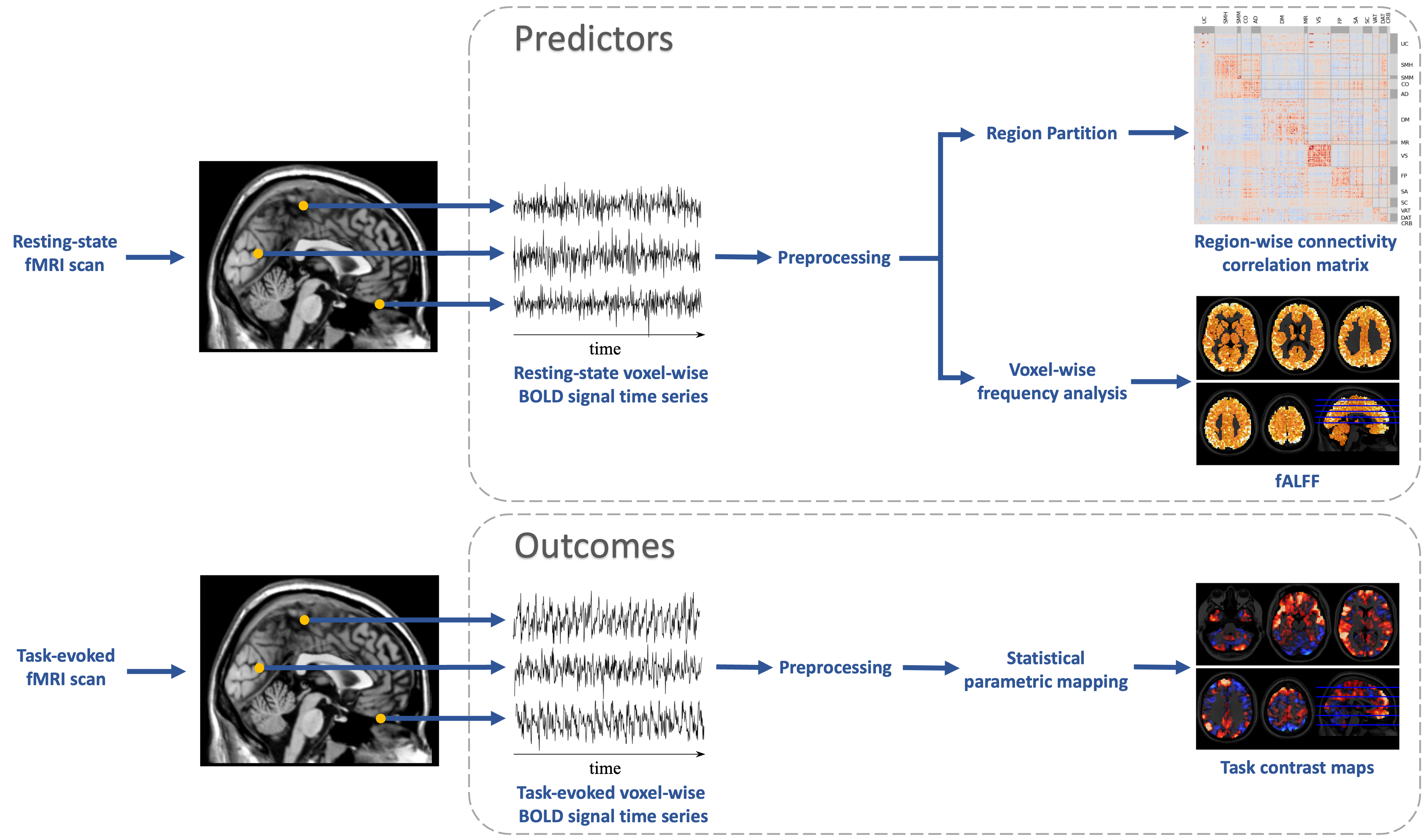
Figure 1: HCP fMRI data pipeline description. From raw fMRI scan, both resting-state and task-evoked blood oxygenation level dependent (BOLD) time series are extracted per participant, which then undergo the HCP minimumally preprocessed pipeline. The preprocessed resting-state images are regionally summarized, yielding connectivity matrices, while voxel-level frequency analysis provides fALFF values. The preprocessed task-evoked BOLD signals undergo statistical parametric mapping, generating task-related contrast maps.

Statistical inference on IIR for neuroimaging studies is challenging due to the high dimensionality of model parameters and the heterogeneity in activation patterns among individuals. The spatial dependence or correlations among predictors and outcomes can be complex and hard to quantify. In some studies, IIR cannot produce very accurate predictions due to the low signal to noise ratio and relatively small sample sizes. In addition to neuroimaging applications, IIR has attracted growing scientific interests in many other fields such as spatial economics (Gelfand et al.,, 2003), genomics (Morris et al.,, 2011) and computer vision (Santhanam et al.,, 2017), where the modeling, inferences and predictions also face similar challenges.

Different IIR methods have been proposed motivated by different applications. A simple linear regression model (Tavor et al.,, 2016) is adopted to make predictions on the task-based fMRI data using the resting fMRI and structural MRI as predictors. This linear regression method assumes the predictor and outcome images are collected in the same imaging space and partitions the imaging space into multiple subregions. For each subject in the training data, a linear regression model is fitted over voxels within each region. The averaging model fits from the training data is used to predict the task activity of a new subject. This method works well for small datasets but lacks the flexibility to capture complex associations between the predictor and outcome images, and it also ignores spatial correlations among voxels.

The spatial Bayesian latent factor model (SBLF) for IIR (Guo et al.,, 2022) has been proposed recently with successful applications in neuroimaging studies. SBLF introduces the spatial latent factors to make connections between the outcome images and predictor images. It explicitly addresses the spatial dependence in images among voxels and achieves better prediction accuracy in the analysis of the fMRI data. However, SBLF introduces random effects in the model and may suffer the over-fitting issues. In addition, the posterior computation of SBLF is extremely challenging and the current algorithm is inefficient and not scalable for the analysis of the large-scale imaging data.

Deep convolutional neural networks have been widely used for predicting images in computer vision applications. These methods preserve spatial information within the image through the use of convolutional layers. Most algorithms using deep convolutional neural networks tend to be developed for specific tasks (Santhanam et al.,, 2017). These tend to make use of the visual geometry group (VGG) and the residual neural network (ResNet) architecture, which is prone to include unnecessary information in the image that biases prediction images (Isola et al.,, 2017). A method has been developed for use in general image-to-image regression problems, called the Recursively Branched Deconvolutional Network (RBDN), which extracts features to form a composite map that is run through several convolutional layers for each task (Santhanam et al.,, 2017). However, this method requires input and output images have the same size, which may not be suitable for all tasks, and it uses the mean-squared error as the objective function which may not be optimal for neuroimaging given that there has not yet been a widely-accepted objective function for each task (Isola et al.,, 2017), including the prediction of fMRI images.

Generative adversarial networks (GANs) have also been applied to image-to-image regressions. In general, GANs avoid the problem of no widely-accepted objective function for image-to-image regression tasks by having the neurons compete to improve the prediction of images in these tasks (Isola et al.,, 2017). A problem is that GANs often lack the ability to directly link the predicted image to the predictor image (Huang et al.,, 2018). This is overcome by the use of conditional GANs to aid mapping random noise to the predicted image (Isola et al.,, 2017). One such method, Pix2Pix, is noted to generate much more sharp images than others (Huang et al.,, 2018). Other methods may couple GAN with a discriminator such as a variational autoencoder (VAE) to improve predictions (Huang et al.,, 2018). But a problem with GANs lies in their objective functions. Among technical problems such as the possibility of reaching Nash equilibrium between competing neurons preventing predictions (Huang et al.,, 2018) and possible saturation of the objective function preventing learning the model from a zero gradient in some cases (Huang et al.,, 2018), GANs in general require much work to properly train. Further, the lack of a specific objective function may prevent the identification by humans of features that are relevant to predictions, which hinders the scientific utility of GANs on task-rest studies of fMRI images.

Of particular importance to new machine learning techniques is the interpretability (Carvalho et al.,, 2019). For methods to be useful in scientific inquiries on task-rest experiments, the model used should show how task image predictions are made from rest images. While there is literature on interpretable GANs (Härkönen et al.,, 2020) and convolutional neural networks (CNNs) (Zhang et al.,, 2018), there is a paucity of literature on IIR methods with interpretability. This limits the use of these methods for task-rest experiments.

To address the challenges of IIR and the limitations of the current methods for neuroimaging applications, in this article, we develop a Bayesian Image-on-image Regression via Deep kernel learning based Gaussian Processes (BIRD-GP). BIRD-GP is a new Bayesian hierarchical model for IIR by integrating deep neural networks (DNN) and Gaussian processes (GP) with kernel learning. It is a framework with two-stage analysis: the image projection via the basis expansion approach (Stage 1) and the nonlinear regression via DNN (Stage 2). This framework substantially reduces the number of model parameters compared to other deep learning methods but it still has the flexibility to capture complex associations between the predictor and outcome images, leading to interpretable model fitting and accurate prediction performances. We propose a novel method to learn the covariance kernel or equivalently the orthonormal basis functions of the GPs via DNN. BIRD-GP can capture detailed characteristics of the predictor and outcome images, substantially facilitate the statistical efficiency in estimating the model parameters, and explicitly provide a set of basis images that can greatly improve interpretability. Under the Bayesian framework, BIRD-GP can also produce valid prediction uncertainty measures via the posterior probability. For posterior computation, we develop a hybrid posterior computation algorithm by combining the Gibbs sampler and the Stein variational gradient descent method. It is computationally efficient and scalable to large scale neuroimaging data. It also can be straightforwardly implemented in parallel.

We conduct extensive experiments to evaluate the performance of BIRD-GP, employing synthetic datasets based on MNIST and Fashion MNIST. BIRD-GP outperformed all competing methods in these experiments. Furthermore, we apply BIRD-GP to two IIR tasks to regress the language task story-math contrast maps and the social recognition random-baseline contrast maps using fALFF images and connectivity correlation matrix from the HCP 1200 release  (WU-Minn HCP,, 2017). Our findings reveal that the language task story-math contrast maps are more predictable than the social recognition random-baseline contrast maps when using fALFF and connectivity as predictors. Additionally, we observe that connectivity alone demonstrated superior predictability compared to fALFF alone in both tasks. However, the combination of both modalities yield the best prediction performance. To gain further insights, we visualize and analyze the basis images generated by BIRD-GP using different modalities as predictors for both tasks.

The rest of the paper is structured as follows. In Section 2, we first provide the model formulation in Section 2.1 and develop the framework of projected predictor image importance calculation in Section 2.2, followed by an equivalent model representation in Section 2.3. Then, in Section 2.4 we describe a novel approach of kernel learning via Deep Neural Networks (DNNs). We discuss the prior specifications in Section 2.5. In Section 3, we describe the posterior algorithm. We present the results of BIRD-GP and competing methods on synthetic datasets in Section 4. We analyze the HCP fMRI data in Section 5, and conclude the paper in Section 6.

2 Method

Suppose the data consists of $n$ observations of the predictor and outcome images. Let $d_{x}$ and $d_{y}$ be the dimension of voxels (or pixels) for the predictor and outcome images, respectively. Let $\mathcal{R}_{x}\subset\mathbb{R}^{d_{x}}$ and $\mathcal{R}_{y}\subset\mathbb{R}^{d_{y}}$ be the collections of voxels to measure image intensities accordingly. For each observation $i$ $(i=1,\ldots,n)$, let $X_{i}(v)$ represent the intensity at voxel $v\in\mathcal{R}_{x}$ and $Y_{i}(u)$ represent the intensity at voxel $u\in\mathcal{R}_{y}$, respectively.

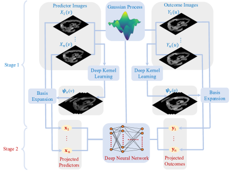
Figure 2: The illustration of BIRD-GP which consists of two stages of analysis. Stage 1: image projection models with the basis expansion approach. Stage 2: deep neural network model for complex associations between projected predictor images and outcome images

2.1 Bayesian image-on-image regression

To model the associations between the predictor and outcome images, we consider a two-stage Bayesian method illustrated in Figure 2. In Stage 1, we model both the predictor and outcome images by a basis expansion approach. We will show our model implies both the predictor and outcome images are realizations of GPs in Section 2.3. Let $\boldsymbol{\psi}_{x}(\cdot)=\{\psi_{x,1}(\cdot),\ldots,\psi_{x,K_{x}}(\cdot)\}^{\top}:\mathcal{R}_{x}\mapsto\mathbb{R}^{K_{x}}$ be a vector of $K_{x}$ orthonormal basis functions for the predictor images, and $\boldsymbol{\psi}_{y}(\cdot)=\{\psi_{y,1}(\cdot),\ldots,\psi_{y,K_{y}}(\cdot)\}^{\top}:\mathcal{R}_{y}\mapsto\mathbb{R}^{K_{y}}$ be a vector of $K_{y}$ orthonormal basis functions for the outcome images. We have $\sum_{v\in\mathcal{R}_{x}}\boldsymbol{\psi}_{x}(v)\boldsymbol{\psi}_{x}^{\top}(v)=\mathbf{I}_{K_{x}}$ and $\sum_{u\in\mathcal{R}_{y}}\boldsymbol{\psi}_{y}(u)\boldsymbol{\psi}_{y}^{\top}(u)=\mathbf{I}_{K_{y}}$ where $\mathbf{I}_{K_{x}}$ is an identity matrix with dimensions $K_{x}\times K_{x}$. We assume

$$X_{i}(v) =\mathbf{x}_{i}^{\top}\boldsymbol{\psi}_{x}(v)+\epsilon_{x,i}(v),\quad\epsilon_{x,i}(v)\sim\mathrm{N}(0,\sigma^{2}_{x,i}),$$ (1)

$$Y_{i}(u) =\mathbf{y}_{i}^{\top}\boldsymbol{\psi}_{y}(u)+\epsilon_{y,i}(u),\quad\epsilon_{y,i}(u)\sim\mathrm{N}(0,\sigma^{2}_{y,i}),$$ (2)

where $\mathbf{x}_{i}\in\mathbb{R}^{K_{x}}$ and $\mathbf{y}_{i}\in\mathbb{R}^{K_{y}}$ represent the $i$th projected predictor image and the $i$th projected outcome image in the corresponding Euclidean vector spaces, respectively. The random noises $\epsilon_{x,i}(v)$ and $\epsilon_{y,i}(u)$ explain the variations of observed images that cannot be explained by the basis functions. We assume that $\epsilon_{x,i}(v)$ and $\epsilon_{y,i}(u)$ are mutually independent across $i$, $v$ and $u$. The variances $\sigma_{x,i}^{2}$ and $\sigma^{2}_{y,i}$ are image-specific and can be different across different images to accommodate the heterogeneity in noises. In Stage 2, we specify the joint distributions of the projected predictor images $\mathbf{x}_{i}$ and the projected outcome images $\mathbf{y}_{i}$. We adopt a feed-forward deep neural network (DNN) to model their complex associations,

$$\mathbf{x}_{i} \sim\mathrm{N}(\boldsymbol{0}_{K_{x}},\boldsymbol{\Lambda}_{x}),\quad(\mathbf{y}_{i}\mid\mathbf{x}_{i})\sim\mathrm{N}\{\mathscr{N}(\mathbf{x}_{i};\boldsymbol{\theta}_{xy}),\boldsymbol{\Lambda}_{y}\},$$ (3)

where $\boldsymbol{0}_{K_{x}}$ is an all-zero vector of length $K_{x}$; covariances $\boldsymbol{\Lambda}_{x}=\mathrm{diag}\{\lambda_{x,1},...,\lambda_{x,K_{x}}\}$ and $\boldsymbol{\Lambda}_{y}=\mathrm{diag}\{\lambda_{y,1},...,\lambda_{y,K_{y}}\}$ are diagonal matrices with positive elements approximating the eigenvalues of the GPs for the predictor and outcome images, respectively. The conditional expectation of $\mathbf{y}_{i}$ given $\mathbf{x}_{i}$ is modeled as an $L$-layer feed-forward DNN $\mathscr{N}(\cdot\,;\boldsymbol{\theta}_{xy}):\mathbb{R}^{K_{x}}\mapsto\mathbb{R}^{K_{y}}$, where each layer has $S_{xy,\ell}$ hidden units ($\ell=0,1,\ldots,L$). The output layer dimension $S_{xy,L}=K_{y}$ and the input layer dimension $S_{xy,0}=K_{x}$, and $\boldsymbol{\theta}_{xy}=\{\mathbf{W}_{xy,\ell},\mathbf{b}_{xy,\ell}\}_{\ell=1}^{L}$ with $\mathbf{W}_{xy,\ell}\in\mathbb{R}^{S_{xy,\ell}\times S_{xy,\ell-1}}$ and $\mathbf{b}_{xy,\ell}\in\mathbb{R}^{S_{xy,\ell}}$.

2.2 Projected predictor image importance

To determine the importance of each element of the projected predictor image $\mathbf{x}$, we consider the log density of the outcome $\mathbf{y}$ given the predictor $\mathbf{x}$, i.e. $\log p(\mathbf{y}\mid\mathbf{x},\boldsymbol{\theta}_{xy},\boldsymbol{\Lambda}_{y})$, and define an importance function by the expectation of its derivative

$$\mathbf{q}(\mathbf{x},\mathbf{y})=\mathbb{E}_{(\boldsymbol{\theta}_{xy},\boldsymbol{\Lambda}_{y})\sim p(\boldsymbol{\theta}_{xy},\boldsymbol{\Lambda}_{y}\mid\mathcal{D})}\frac{\partial}{\partial\mathbf{x}}\log p(\mathbf{y}\mid\mathbf{x},\boldsymbol{\theta}_{xy},\boldsymbol{\Lambda}_{y}),$$

where the derivative and expectation is exchangeable and $\mathbf{q}:\mathbb{R}^{K_{x}}\times\mathbb{R}^{K_{y}}\mapsto\mathbb{R}^{K_{x}}$ is a function of $\mathbf{x}$ and $\mathbf{y}$ in general and its output dimension is the same as the dimension of $\mathbf{x}$. We would like to note that $\mathbf{q}(\mathbf{x},\mathbf{y})$ provides a lower bound of the derivative of the log of the posterior predictive distribution, i.e., $\log p(\mathbf{y}\mid\mathbf{x},\mathcal{D})$, w.r.t. $\mathbf{x}$ by the Jensen’s inequality, where $\mathcal{D}$ denotes training data of projected predictor and outcome images. This connection is an analogy of the log marginal density of data and evidence lower bound (ELBO) in the variational inference context. Then we define the importance of the projected predictor image by taking the expectation of the absolute value of $\mathbf{q}(\mathbf{x},\mathbf{y})$, i.e.,

$$\textbf{IM}=\mathbb{E}\left|\mathbf{q}(\mathbf{x},\mathbf{y})\right|=\int\left|\mathbf{q}(\mathbf{x},\mathbf{y})\right|p(\mathbf{x},\mathbf{y}\mid\mathcal{D})\;d\mathbf{x}d\mathbf{y},$$ (4)

where $|\cdot|$ is an element-wise absolute value function. The expectation is taken with respective to the joint predictive distribution of $\mathbf{x}$ and $\mathbf{y}$, i.e. $p(\mathbf{x},\mathbf{y}\mid\mathcal{D})=p(\mathbf{y}\mid\mathbf{x},\mathcal{D})p(\mathbf{x}\mid\mathcal{D})$ Note that IM is a vector of length $K_{x}$, where each element is the importance measure of the corresponding dimension of the projected predictor image $\mathbf{x}$ for prediction.

As a simple illustration, suppose $(\mathbf{y}\mid\mathbf{x})\sim\mathrm{N}(\boldsymbol{\theta}_{xy}\mathbf{x},\boldsymbol{\Lambda}_{y})$ where $\mathbf{x}$, $\mathbf{y}$, $\boldsymbol{\theta}_{xy}$ and $\boldsymbol{\Lambda}_{y}$ are all scalers. We assume further that the posterior distribution of $\boldsymbol{\theta}_{xy}$ and $\boldsymbol{\Lambda}_{y}$ are degenerate, so that $\boldsymbol{\theta}_{xy}$ can only take $\beta\in\mathbb{R}$ and $\boldsymbol{\Lambda}_{y}$ can only take $\lambda_{y}\in\mathbb{R}^{+}$. Then, the importance function $\mathbf{q}(\mathbf{x},\mathbf{y})=\frac{\partial}{\partial\mathbf{x}}\log\mathrm{N}(\mathbf{y}\mid\beta\mathbf{x},\lambda_{y})$ and the importance measure of $\mathbf{x}$ is $\textbf{IM}=\mathbb{E}_{\mathbf{x},\mathbf{y}}\left|\frac{\partial}{\partial\mathbf{x}}\log\mathrm{N}(\mathbf{y}\mid\beta\mathbf{x},\lambda_{y})\right|=\frac{|\beta|}{\lambda_{y}}\mathbb{E}_{\mathbf{x},\mathbf{y}}\left|\mathbf{y}-\beta\mathbf{x}\right|=\frac{|\beta|}{\lambda_{y}}\mathbb{E}_{\mathbf{x}}\mathbb{E}_{\mathbf{y}\mid\mathbf{x}}\left|\mathbf{y}-\beta\mathbf{x}\right|=\frac{|\beta|}{\lambda_{y}}\mathbb{E}_{\mathbf{x}}\lambda_{y}\sqrt{\frac{2}{\pi}}=\sqrt{\frac{2}{\pi}}|\beta|$ by noting that $\mathbb{E}_{\mathbf{y}\mid\mathbf{x}}\left|\mathbf{y}-\beta\mathbf{x}\right|$ is the expectation of a half-normal random variable. With a linear model, the importance of $\mathbf{x}$ is its coefficient magnitude scaled by a factor.

In practice, the closed-form representation of (4) may not be available as in the linear model example, but we can approximate IM via the Monte Carlo method. Suppose we have $S$ samples of $\boldsymbol{\theta}_{xy}$ and $\boldsymbol{\Lambda}_{y}$ drawn from their posterior distributions, denoted as $\{(\boldsymbol{\theta}^{(s)}_{xy},\boldsymbol{\Lambda}^{(s)}_{y})\}_{s=1}^{S}$, and denote $n^{*}$ pairs of projected predictor and outcome images by $\{(\mathbf{x}^{*}_{i},\mathbf{y}_{i}^{*})\}_{i=1}^{n^{*}}$ . Then, we estimate IM by

$$\widehat{\textbf{IM}}=\frac{1}{n^{*}}\sum_{i=1}^{n^{*}}\left|\widehat{\mathbf{q}}(\mathbf{x}^{*}_{i},\mathbf{y}_{i}^{*})\right|,\quad\widehat{\mathbf{q}}(\mathbf{x}^{*}_{i},\mathbf{y}_{i}^{*})=\frac{1}{S}\sum_{s=1}^{S}\frac{\partial}{\partial\mathbf{x}}\log p(\mathbf{y}_{i}^{*}\mid\mathbf{x},\boldsymbol{\theta}^{(s)}_{xy},\boldsymbol{\Lambda}^{(s)}_{y})\Big{|}_{\mathbf{x}=\mathbf{x}_{i}^{*}}.$$ (5)

Of note, the function $\frac{\partial}{\partial\mathbf{x}}\log p(\mathbf{y}\mid\mathbf{x},\boldsymbol{\theta}_{xy},\boldsymbol{\Lambda}_{y})$ can be efficiently evaluated by using the automatic differentiation algorithm for the deep neural network model. In addition, $(\mathbf{x}^{*}_{i},\mathbf{y}^{*}_{i})$ may represent new data different from the training data $\mathcal{D}$. When the new data is not available, $(\mathbf{x}_{i}^{*},\mathbf{y}_{i}^{*})$ can be drawn from $\mathcal{D}$.

2.3 Equivalent model representation

Combining (1), (2) and (3), we obtain an equivalent model representation for a better interpretation of the predictor and outcome images in the original space. It is straightforward to show that the predictor images are realizations of GP from (1),

$$X_{i}(v)\sim\mathcal{GP}\{0,\kappa_{x,i}(v,v^{\prime})\},$$ (6)

where the mean function of the GP is 0 and the kernel function $\kappa_{x,i}(v,v^{\prime})=\sum_{k=1}^{K_{x}}\lambda_{x,k}\psi_{x,k}(v)\psi_{x,k}(v^{\prime})+\sigma^{2}_{x,i}I(v=v^{\prime})$ for any $v,v^{\prime}\in\mathcal{R}_{x}$. To represent the conditional distribution of $Y_{i}(v)$ given $X_{i}(v)$, we introduce random effects $\mathbf{e}_{i}=-\sum_{v\in\mathcal{R}_{x}}\epsilon_{x,i}(v)\boldsymbol{\psi}_{x}(v)$. By the property of $\boldsymbol{\psi}_{x}(v)$ and distribution of $\epsilon_{x,i}$, we have that

$$\mathbf{x}_{i}=\sum_{v\in\mathcal{R}_{x}}\boldsymbol{\psi}_{x}(v)X_{i}(v)+\mathbf{e}_{i},\quad\mathbf{e}_{i}\sim\mathrm{N}(\boldsymbol{0},\sigma^{2}_{x,i}\mathbf{I}_{K_{x}}).$$ (7)

This further implies that the conditional expectation of $Y_{i}(u)$ given $\{X_{i}(v)\}_{v\in\mathcal{R}_{x}}$, denoted as $\mu_{i}(u)$, can be constructed by integrating out $\mathbf{e}_{i}$ in the model. In particular,

$$\mu_{i}(u)=\mathbb{E}_{\mathbf{e}_{i}}\Big{\{}\mathscr{N}\Big{(}\sum_{v\in\mathcal{R}_{x}}\boldsymbol{\psi}_{x}(v)X_{i}(v)+\mathbf{e}_{i};\boldsymbol{\theta}_{xy}\Big{)}\Big{\}}^{\top}\boldsymbol{\psi}_{y}(u),$$ (8)

where the expectation is taken with respect to $\mathbf{e}_{i}$. Furthermore, by the independence of $\epsilon_{x,i}(v)$ and $\epsilon_{y,i}(u)$, we have

$$[Y_{i}(u)\mid\{X_{i}(v)\}_{v\in\mathcal{R}_{x}}]\sim\mathcal{GP}\{\mu_{i}(u),\kappa_{y,i}(u,u^{\prime})\},$$ (9)

where kernel $\kappa_{y,i}(u,u^{\prime})=\sum_{k=1}^{K_{y}}\lambda_{y,k}\psi_{y,k}(u)\psi_{y,k}(u^{\prime})+\sigma^{2}_{y,i}I(u=u^{\prime})$ for any $u,u^{\prime}\in\mathcal{R}_{y}$. We provide the derivations of the equivalent model representation in Section S1 in the Supplementary Materials.

2.4 Kernel learning via DNN

The accuracy of approximating images using GPs largely depends on the flexibility of the covariance kernel. Under our framework, it is straightforward to use fixed kernels such as the squared-exponential (SE) and the Matérn kernel. However, such kernels lack the flexibility to explain complex spatial structures in practice. Therefore, we develop a novel DNN-based data adaptive method to estimate the eigenfunctions and construct the covariance kernel of GPs in (6) and (9). We only illustrate our method on the construction of $\boldsymbol{\psi}_{x}(v)$ for predictor images. A similar approach can be applied to outcome images. For $v\in\mathcal{R}_{x}$, let $\mathbf{X}(v)=\{X_{1}(v),\ldots,X_{n}(v)\}^{\top}$ be a vector of $n$ observed predictor image measurements at voxel $v$. To approximate $\mathbf{X}(v)$, we introduce a feed-forward DNN $\mathscr{N}(v;\boldsymbol{\theta}_{x}):\mathbb{R}^{d_{x}}\mapsto\mathbb{R}^{K_{x}}$, where the dimension of the input layer is the dimension of the predictor image voxel $d_{x}$ and the dimension of the output layer is the number of orthonormal basis functions $K_{x}$. Note that the DNN here for kernel learning is different from the one we use in (3). Then we adopt the linear transformation to project $\mathscr{N}(v;\boldsymbol{\theta}_{x})$ onto $\mathbb{R}^{n}$ for approximating $\mathbf{X}(v)$. We solve the following optimization problem,

$$(\hat{\mathbf{P}}_{x},\hat{\boldsymbol{\theta}}_{x})=\underset{(\mathbf{P}_{x},\boldsymbol{\theta}_{x})}{\arg\min}\sum_{v\in\mathcal{R}_{x}}\big{\|}\mathbf{X}(v)-\mathbf{P}_{x}\mathscr{N}(v;\boldsymbol{\theta}_{x})\big{\|}^{2}_{2},$$ (10)

where $\mathbf{P}_{x}\in\mathbb{R}^{n\times K_{x}}$ is the linear projection matrix. The estimated DNN function $\mathscr{N}(v;\hat{\boldsymbol{\theta}}_{x})$ can be considered as a vector of $K_{x}$ unorthonormalized basis functions. To construct $\boldsymbol{\psi}_{x}(v)$, for general $\mathcal{R}_{x}$, we can apply the Gram-Schmidt process on $\mathscr{N}(v;\hat{\boldsymbol{\theta}}_{x})$ for orthonormalization. When $\mathcal{R}_{x}$ contains a finite number of equal space grid points, we use the Singular Value Decomposition on matrix $\{\mathscr{N}(v;\hat{\boldsymbol{\theta}}_{x})\}_{v\in\mathcal{R}_{x}}$ to obtain the orthonormal matrix $\{\boldsymbol{\psi}_{x}(v)\}_{v\in\mathcal{R}_{x}}$.

Note that the classical Principle Component Analysis (PCA) can decompose the observed images and provide a set of orthonormal basis functions but is subject to noise and is prone to overfit. However, learning the kernel via DNNs, our approach implicitly imposes smoothness constraints and is more robust. Furthermore, we may add regularization terms to the objective function or apply dropout layers (Srivastava et al.,, 2014) to prevent overfitting. Another advantage of our approach over PCA is that we learn the kernel as a function so that it is possible to interpolate or extrapolate kernel function values, while PCA only provides the value of the kernel function evaluated at fixed locations.

2.5 Prior specifications

Given the estimated orthonormal basis functions for predictor images and outcomes $\boldsymbol{\psi}_{x}(v)$ and $\boldsymbol{\psi}_{y}(u)$, we perform Bayesian inferences on the proposed model. For the weight and bias parameters of the DNN model in (3), we assign independent normal priors, i.e., for $\ell=1,\ldots,L$ $\mathrm{vec}(\mathbf{W}_{xy,\ell})\sim\mathrm{N}(\boldsymbol{0},\sigma^{2}_{w}\mathbf{I}_{S_{xy,\ell}\times S_{xy,\ell-1}})$,$\mathbf{b}_{xy,\ell}\sim\mathrm{N}(\boldsymbol{0},\sigma^{2}_{w}\mathbf{I}_{S_{xy,\ell}}),$ where $\sigma^{2}_{w}$ is the prior variance parameters for the weight and bias parameters. For all the variance parameters in the model, we assign inverse gamma priors , i.e., for $i=1,\ldots,n$, $k_{x}=1,\ldots,K_{x}$ and $k_{y}=1,\ldots,K_{y}$, we have $\sigma^{2}_{x,i},\sigma^{2}_{y,i}\sim\mathrm{IG}(a_{\sigma},b_{\sigma})$, $\sigma^{2}_{w}\sim\mathrm{IG}(a_{w},b_{w})$, $\lambda_{x,k_{x}},\lambda_{x,k_{y}}\sim\mathrm{IG}(a_{\lambda},b_{\lambda})$, where all the shape and scale parameters in the inverse gamma distributions are pre-specified. In practice, we suggest to set $a_{\sigma}=b_{\sigma}=a_{\lambda}=b_{\lambda}=a_{w}=1$. While suitable $b_{w}$ may vary across different datasets, we suggest $b_{w}$ take value from 1 to 100. We provide sensitivity analysis in Supplementary Materials S2, showing that mild changes in hyperparameters will not lead to a drastic decrease in the model performance.

3 Posterior Computation

To ensure the efficiency and scalability of BIRD-GP, we develop a two-stage hybrid posterior computation algorithm. The two-stage algorithm is efficient in terms of both time and memory. The computational bottleneck resides in the projection of high-dimensional images onto the low-dimensional Euclidean space, which can be greatly mitigated by Stage 1 posterior computation that can be straightforwardly paralleled across subjects. In Stage 1, we apply the Gibbs sampler for Bayesian linear regressions (1) and (2) to simulate the posterior distribution of the projected predictor image $\mathbf{x}_{i}$ and outcome image $\mathbf{y}_{i}$ along with associated variance parameters $\boldsymbol{\Lambda}_{x}$, $\boldsymbol{\Lambda}_{y}$, $\sigma^{2}_{x,i}$ and $\sigma^{2}_{y,i}$ given all other parameters.

  Draw $S$ random samples from the prior distribution: $\boldsymbol{\Theta}^{0}_{1},\ldots,\boldsymbol{\Theta}^{0}_{S}$.

  Update $\{\boldsymbol{\Theta}^{0}_{s}\}_{s=1}^{S}$ for $T$ iterations

  for $t$ in $0:(T-1)$ do

     Sample indices $\mathcal{I}\subset[n]=\{1,\ldots,n\}$

     for $s$ in $1:S$ do

        Compute $\boldsymbol{\Theta}^{t+1}_{s}$ given $\boldsymbol{\Theta}^{t}_{1},\ldots,\boldsymbol{\Theta}^{t}_{S}$ and the subset of projected images $\mathbf{D}_{\mathcal{I}}$ via (11)

     end for

  end for

Algorithm 1 SVGD for Bayesian neural networks

In Stage 2, we adopt the Stein Variational Gradient Descent Algorithm (SVGD) (Liu and Wang,, 2016) to simulate the posterior distribution of all the parameters that are associated with the DNN model in (3), i.e., $\boldsymbol{\Theta}=\{\boldsymbol{\theta}_{xy},\sigma^{2}_{w},\sigma^{2}_{b}\}$. As a gradient-based method, SVGD provides a general variational inference framework. Let $\mathbf{D}_{\mathcal{I}}=\big{\{}\mathbb{E}[\mathbf{x}_{i}\,|\,X_{i}(v)],\,\mathbb{E}[\mathbf{y}_{i}\,|$ $Y_{i}(u)]\big{\}}_{i\in\mathcal{I}}$ represent a collection of posterior mean of the projected predictor images and the projected outcome images with indices in $\mathcal{I}\subset[n]=\{1,\ldots,n\}$. Denote by $q(\boldsymbol{\Theta})$ and $p(\boldsymbol{\Theta}\,|\,\mathbf{D}_{\mathcal{I}})$ the prior distribution and the posterior distribution of $\boldsymbol{\Theta}$ given data $\mathbf{D}_{\mathcal{I}}$, respectively. The first step is to draw $S$ random samples from the prior $q(\boldsymbol{\Theta})$, denoted as $\{\boldsymbol{\Theta}_{s}^{0}\}_{s=1}^{S}$. Then we iteratively update the samples of $\boldsymbol{\Theta}$ from the prior towards the posterior distribution using the stochastic gradient descent (SGD) algorithm. Specifically, at the $(t+1)$th iteration $(t=0,\ldots,T-1)$, we first sample $\mathcal{I}\subset[n]$; then for $s=1,\ldots,S$, we update the $s$th sample of $\boldsymbol{\Theta}$, denoted by $\boldsymbol{\Theta}^{t}_{s}$, by the following rule,

$$\boldsymbol{\Theta}^{t+1}_{s}=\boldsymbol{\Theta}^{t}_{s}+\frac{\alpha}{S}\sum^{S}_{s^{\prime}=1}\bigg{[}k(\boldsymbol{\Theta}^{t}_{s^{\prime}},\boldsymbol{\Theta}^{t}_{s})\big{\{}\nabla_{\boldsymbol{\Theta}^{t}_{s^{\prime}}}\log p(\boldsymbol{\Theta}^{t}_{s^{\prime}}\,|\,\mathbf{D}_{\mathcal{I}})\big{\}}+\big{\{}\nabla_{\boldsymbol{\Theta}^{t}_{s^{\prime}}}k(\boldsymbol{\Theta}^{t}_{s^{\prime}},\boldsymbol{\Theta}^{t}_{s})\big{\}}\bigg{]},$$ (11)

where $\alpha$ is the step size and $k(\cdot,\cdot)$ is the kernel function that defines the Stein discrepancy between the density of $\{\boldsymbol{\Theta}_{s}^{t}\}_{s=1}^{S}$ and the target density $p(\boldsymbol{\Theta}\,|\,\mathcal{D}_{[n]})$. Here, we present the basic SGD algorithm in (11). In practice, one may choose more advanced SGD algorithm such as the Adam optimizer (Kingma and Ba,, 2015). We use the Gaussian kernel $k(x,y)=\exp\big{\{}-\frac{1}{h}\|x-y\|^{2}_{2}\big{\}}$ where $h$ is chosen as the median of the pairwise distance between the current samples $\{\boldsymbol{\Theta}^{t}_{s}\}_{s=1}^{S}$ divided by $\log(n)$ (Liu and Wang,, 2016); the closed-form of $\nabla_{\boldsymbol{\Theta}^{t}_{s^{\prime}}}k(\boldsymbol{\Theta}^{t}_{s^{\prime}},\boldsymbol{\Theta}^{t}_{s})$ is available in this case. We adopt the automatic differentiation approach to compute the gradient of $\log p(\boldsymbol{\Theta}^{t}_{j}\,|\,\mathbf{D}_{\mathcal{I}})$ in practice.

4 Simulations on Synthetic Data

We evaluate the performance of BIRD-GP on synthetic data based on MNIST and Fashion MNIST datasets, and compare BIRD-GP with three DNNs, three CNNs, and the Recursively Branched Deconvolutional Network (RBDN) (Santhanam et al.,, 2017). DNNs and CNNs are with different architectures. Under the BIRD-GP framework, we also compare the DNN-based kernel and other kernel constructions – the squared-exponential (SE) and the Matérn kernel, and the PCA-based kernel. The hyperparameters of all competitors are discussed the Supplementary Materials S3.

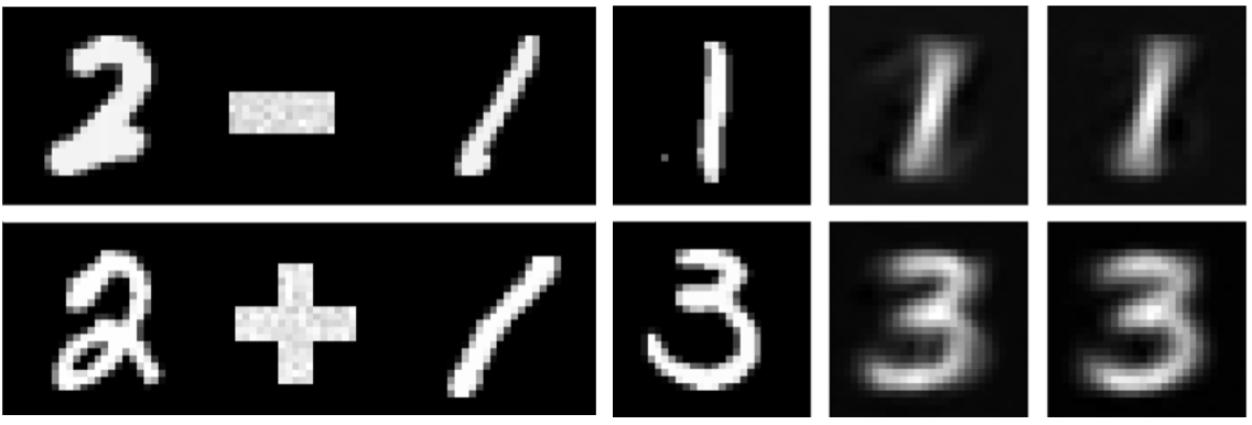
(a) Two test examples from the MNIST experiment. The first two columns show the synthesized predictor images and outcome images. The third column shows the predicted outcomes by BIRD-GP, while the last column is the predicted outcomes by CNN2.

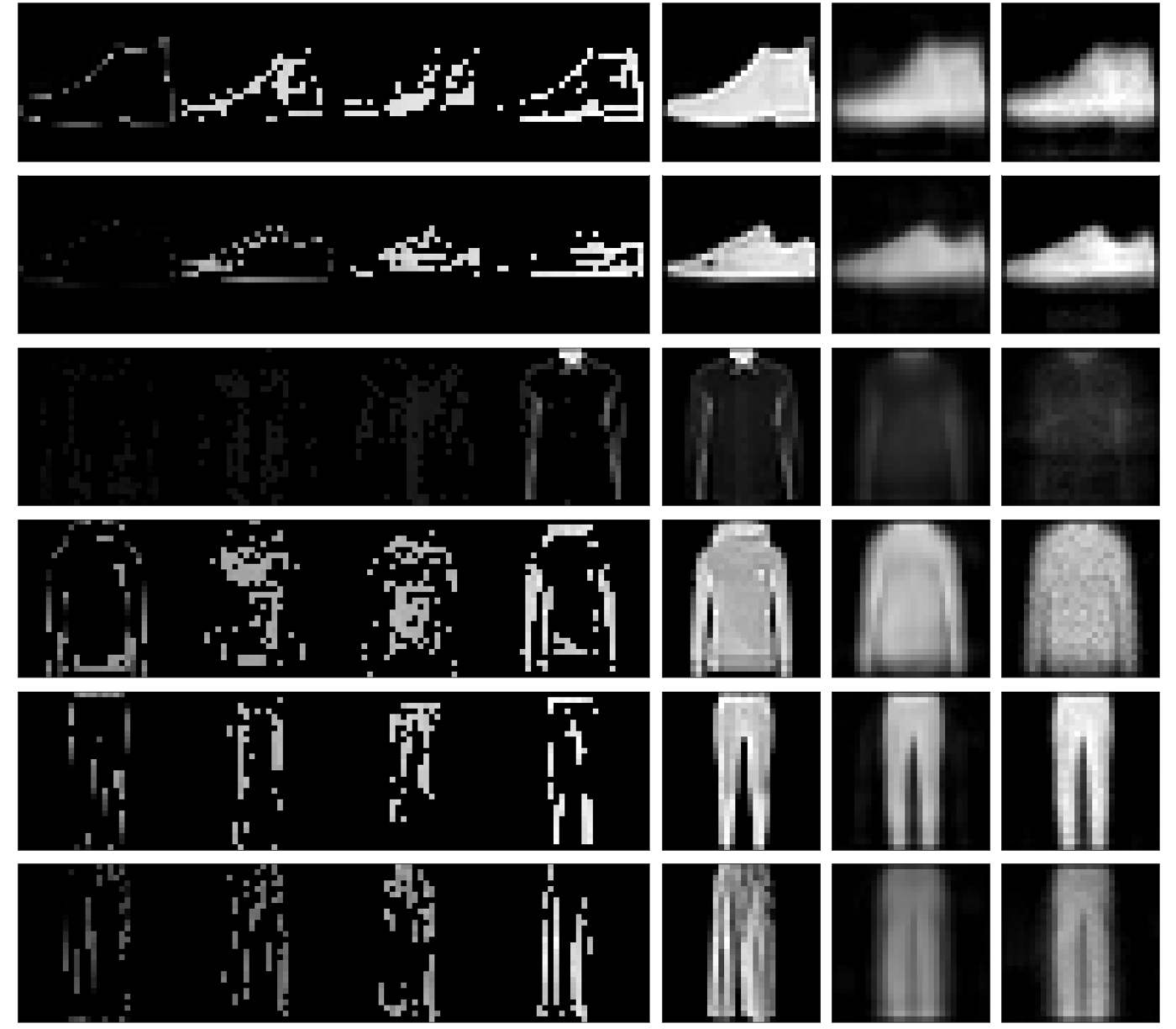
(b) Six test examples from the Fashion MNIST experiment. The first two columns show the synthesized predictor images and outcome images. The third column shows the predicted outcomes by BIRD-GP, while the last column is the predicted outcomes by CNN2.

Figure 3: Example images from the (a) MNIST experiment and (b) Fashion MNIST experiment.

4.1 MNIST

The MNIST handwritten digits dataset (LeCun et al.,, 2010) contains 60,000 training and 10,000 testing image-label pairs. Each image is a $28\times 28$ handwritten digit (0-9). We design the experiment so as to mimic the calculation of “$2+1=3$” and “$2-1=1$”. We synthesize predictor images of size $28\times 84$ based on the MNIST dataset by horizontally stacking an image of “2”, an $28\times 28$ image of either “$+$” or “$-$” and an image of “1”. The plus/minus sign in between are randomly generated with varying margins, widths and lengths. The outcome images are either images of “3” or “1”, depending the sign in the middle of the predictor images. Images of “1”, “2” and “3” in predictors and outcomes are randomly selected without replacement. Figure 3(a) shows two examples from the testing set.

We generate 1,000 training samples and 1,000 testing samples for each dataset and repeat the experiment on 50 datasets. We use the fully trained models to predict the outcome images; the predictions are further fed into a pre-trained CNN binary classifier of MNIST images of “1” and “3”. The pre-trained CNN classifier uses the outcome images for training and testing, and obtains close-to-perfect training and testing accuracy. We evaluate the performance of all models by checking the classification accuracy of the predicted label by the pre-trained classifier given the predicted outcome images, as this is a good indicator of the extent to which the model restores the outcome images.

Table 1: Training and testing performance of BIRD-GP and other competing methods are summarized for (a) MNIST and (b) Fashion MNIST experiments.

(a) Proportions of replicates where classification accuracy is larger than 0.995 for both training and testing synthesized MNIST images. Number of parameters are shown after the model name.

	Training	Testing
BIRD-GP (126K)	1.00	1.00
PCA-BIRD-GP	1.00	0.02
SE-BIRD-GP	0.96	0.96
Matérn-BIRD-GP	1.00	1.00
DNN1 (202K)	0.02	0.00
DNN2 (935K)	0.02	0.00
DNN3 (1001K)	0.02	0.08
CNN1 (168K)	0.92	0.88
CNN2 (99K)	0.60	0.80
CNN3 (225K)	0.88	0.96
RBDN (445K)	1.00	1.00

(b) Mean and standard deviation of training and testing MSE over 50 synthesized datasets based on Fashion MNIST. Number of parameters are shown after the model name.

	Training MSE	Testing MSE
BIRD-GP (126K)	0.0234 (0.0010)	0.0260 (0.0010)
PCA-BIRD-GP	0.0203 (0.0038)	0.0301 (0.0039)
SE-BIRD-GP	0.0356 (0.0011)	0.0379 (0.0009)
Matérn-BIRD-GP	0.0354 (0.0010)	0.0378 (0.0010)
DNN1 (252K)	0.0341 (0.0018)	0.0367 (0.0014)
DNN2 (1136K)	0.0243 (0.0005)	0.0306 (0.0005)
DNN3 (1202K)	0.0238 (0.0004)	0.0310 (0.0005)
CNN1 (193K)	0.0348 (0.0016)	0.0364 (0.0015)
CNN2 (103K)	0.0324 (0.0009)	0.0343 (0.0007)
CNN3 (233K)	0.0267 (0.0008)	0.0300 (0.0007)
RBDN (445K)	0.0307 (0.0041)	0.0475 (0.0053)

(c) Fashion MNIST experiment MSE stratified by image label class (train / test), sorted by testing MSE in descending order.

Label	Bag	Ankle Boot	Sandal	Dress	Coat
MSE	0.0339 / 0.0420	0.0314 / 0.0347	0.0322 / 0.0345	0.0244 / 0.0278	0.0233 / 0.0277
Label	Pullover	T-shirt	Shirt	Trouser	Sneaker
MSE	0.0200 / 0.0252	0.0218 / 0.0248	0.0214 / 0.0230	0.0196 / 0.0226	0.0222 / 0.0222

We use a four-layer neural network with ReLU activation for kernel learning. Each layer has 128 hidden nodes. The number of eigenfunctions is set to be 50 for both predictors and outcomes. For the Bayesian neural network, we adopt a ReLU-activated one-layer structure with 200 neurons. We train the BNN for 30 epochs with batch size 64 by SVGD. The six neural networks are trained for 100 epochs and RBDN is trained for 50 epochs, all with batch size 64. In Table 1(a), we summarize the proportion of experiments where the classification accuracy is larger than 0.995 over the 50 replicates. Both the DNN-based kernel and the Matérn kernel under the BIRD-GP framework achieve training and testing accuracy of at least 0.995 for all datasets. Even with a relatively small number of parameters, BIRD-GP outperforms all CNNs and DNNs. RBDN has similar performance to BIRD-GP, but with much more paramters. The PCA-based kernel performs well on the training set, but has poor performance on the testing set.

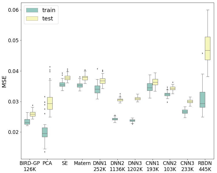
(a)

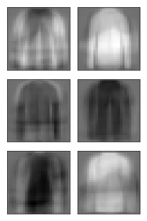
(b)

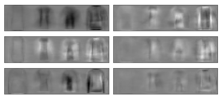
(c)

Figure 4: The Fashion MNIST experiment: (a) The boxplot of training and testing MSE over 50 datasets for the Fashion MNIST experiment. We compare BIRD-GP with other methods. Under the BIRD-GP framework, we consider the DNN-based kernel, the PCA-based kernel, the squared-exponential (SE) kernel and the Matérn kernel. DNN1, DNN2 and DNN3 are deep neural network models with different architectures. CNN1, CNN2 and CNN3 are deep convolutional neural network models with different architectures. RBDN stands for the recursively branched deconvolutional network model. The number of parameters for neural network models are presented below model names. (b) The first 6 outcome basis images with the highest eigenvalues. (c) The first 6 predictor basis images with the highest eigenvalues.

4.2 Fashion MNIST

The Fashion MNIST dataset (Xiao et al.,, 2017) is a gray-scale image dataset containing 10 classes of fashion products. The dataset contains 60,000 training images and 10,000 testing images, each of size $28\times 28$. We synthesize 1,000 training samples and 1,000 testing samples based on the dataset. For each image, we filter four sub-images based on quartiles of non-zero voxel intensities. Each sub-image keeps non-zero voxel intensities within an inter-quartile range, while other voxels are masked to 0. We stack the four sub-images horizontally, with the first inter-quartile image on the left and the fourth inter-quartile image on the right. We treat the stacked image with size $28\times 112$ as the predictor while the original image as the outcome. Figure 3(b) shows six examples from the testing set.

We generate 50 such datasets and compare the MSE on the predictions of outcome images by BIRD-GP and other methods. Training parameters of all methods are the same as Section 4.1. Table 1(b) shows the mean and standard deviation of MSE over 50 replicates. Figure 4(a) shows the boxplot for the training and testing accuracy over 50 replicates. BIRD-GP performs the best on the testing data despite its limiting number of parameters. Figure 3(b) shows BIRD-GP can well capture the individual difference of test outcome images, even with limited training samples. It is worth noting that the PCA-based kernel performs the best on the training data while it is not competitive on the test set, and fixed kernels lack the flexibility to fit the data well.

To demonstrate 50 basis functions are sufficient, we repeat the experiment on the first dataset using 100 basis functions. The first 50 basis account for 95.66% of total variance in the predictor images and 98.37% in the outcome images (see Supplementary Materials S4). Figures 4(c) and 4(b) show the top six basis images with the largest eigenvalues for predictors and outcomes, respectively. We see patterns of shirts, trousers and sneakers in the top basis images. In Table 1(c), we summarize within-class MSEs. BIRD-GP performs better on images whose patterns are detected by the top eigenfunctions, but loses some of its power in other types of images. Finally, to demonstrate our method can measure prediction uncertainty, we compute the mean coverage rates (MCR) of the voxel-wise 95% predictive credible interval for each outcome image. The average of MCR across images is 97.7% (s.d. 1.1%) on the training set and 95.9% (s.d. 3.2%) on the testing set.

5 Analysis of fMRIs in HCP

In this study, we analyze fMRI data from the Human Connectome Project (HCP) 1200 release (Van Essen et al.,, 2012; WU-Minn HCP,, 2017) by BIRD-GP. Previous studies have found that resting-state connectomes exhibit inter-individual differences, which can be attributed to a moderate number of connectivity components and utilized for phenotypic prediction (Sripada et al.,, 2019). One type of resting-state fMRI data, fALFF, has shown to exhibit the ability to predict clinical outcomes (Zhao et al.,, 2015; Egorova et al.,, 2017). On the other hand, task-evoked fMRIs demonstrate variability across individuals and serve as valuable resources for constructing predictive models of General Cognitive Ability (GCA) (Sripada et al.,, 2020). An important question is to determine the extent to which the individual variability in task functional brain activity can be explained by resting-state functional brain activity alone (Tavor et al.,, 2016), connectivity alone, and the combined use of both modalities. It is also of great interest to explore which one of fALFF and connectivity can provide more prediction power for task-evoked brain images. To address this inquiry, we undertake an IIR analysis, where we regress task fMRI contrast maps on fALFF images and connectivity matrices.

We focus on two types of task fMRI contrast maps as outcome images: language task story-math contrast maps and social recognition task random-baseline contrasts maps. For each outcome type, we explore three types of predictors: fALFF alone, connectivity alone, and a combination of both modalities. Additionally, we take into account available confounders, such as age, gender, and race, in our analysis whenever possible.

5.1 Data description and data processing

All data analyzed in this study are from the HCP-1200 release. Data collections and analyses are performed in accordance with relevant guidelines and regulations. Figure 1 describes the predictors and outcomes in our study.

The HCP language task involves two runs, with each run interleaving 4 blocks of story tasks and 4 blocks of math tasks. During the story blocks, participants are exposed to brief auditory stories adapted from Aesop’s fables (5-9 sentences). Following each story, a forced two-option question prompts the participants about the topic of the story. The math blocks entail completing addition and subtraction problems. Detailed task descriptions can be found in previous works (Binder et al.,, 2011; WU-Minn HCP,, 2017). The HCP social recognition task consists of two runs, each comprising 5 video blocks (2 mental and 3 random in one run, 3 mental and 2 random in the other run) and 5 fixation blocks (15 seconds each). The videos feature 20-second clips of objects (e.g., squares, circles, triangles) either interacting in a specific manner (mental) or moving randomly (random) on the screen. After each video, participants are asked to judge whether the objects have a mental interaction, not sure, or no interaction. Detailed task information can be found in works by Castelli et al., (2000), Wheatley et al., (2007) and WU-Minn HCP, (2017).

During the tasks, fMRI data is collected using a 32-channel head coil on a 3T Siemens Skyra scanner (TR = 720 ms, TE = 33.1 ms, 72 slices, 2 mm isotropic voxels, multiband acceleration factor = 8) with right-to-left and left-to-right phase encoding directions. Statistical parametric mapping via general linear regressions is then employed to obtain the story versus math contrast (story-math) and random versus fixation or baseline contrast (random). The data is preprocessed using the HCP minimally preprocessed pipeline (Glasser et al.,, 2013), which includes gradient unwrapping, motion correction, field map distortion correction, brain-boundary based linear registration of functional to structural images, nonlinear registration to MNI152 space, and grand-mean intensity normalization. Data are then processed by a surfaced-based stream and grayordinate-based processing (Glasser et al.,, 2013; Sripada et al.,, 2020). Both task contrast maps are obtained using statistical parametric mapping by general linear regressions (Lindquist,, 2008). All fALFF, story-math and random contrast map outcome images are registered into the MNI (2mm) (Evans et al.,, 1993) standard brain template with a resolution of $91\times 109\times 91$.

The resting-state connectivity correlation matrix is derived from four timecourse files collected from two different fMRI sessions, each comprising 264 nodes. The 264 nodes are divided into 13 functional modules (Power et al.,, 2011), see Supplementary Materials S5. In each session, participants complete two consecutive resting-state sessions lasting approximately 15 minutes each. The participant-specific connectivity correlation matrix is then calculated by averaging the Fisher’s Z-transformed correlation matrix for the subject over the four runs.

Our analysis includes data from 714 subjects who possess all modalities (fALFF, connectivity, story-math, and random) as well as available confounders (age, gender, and race).

Table 2: Predictive results in selected regions of four models for the language tasks and social recognition task (random). All four models use fALFF as predictors. Model name ending with c means the model adjusts for confounders. LR stands for linear regression and VR stands for voxelwise regression. We summarize the proportion of predictable voxels in (a), and their mean and IQR of average predictive $\bar{R^{2}}$ in (b) and (c), respectively. All results are based on the 100 train/test splits. Since fALFF alone does not provide enough prediction power, a region is selected if it has at least 5% predictable voxels by two models or at least 20% predictable voxels by one model.

(a) Proportion of predictable voxels.

Task	Region	LR	VR	VRc	BIRD-GPc
Language	Temporal_Pole_Mid_R	–	$3.0\%$	$7.1\%$	$6.7\%$
Social	Parietal_Sup_R	$0.1\%$	$3.5\%$	$4.2\%$	$21.6\%$
	Calcarine_L	$2.3\%$	$3.8\%$	$5.6\%$	$6.6\%$

(b) Mean of the average predictive $\bar{R^{2}}$ over 100 splits of predictable voxels.

Task	Region	LR	VR	VRc	BIRD-GPc
Language	Temporal_Pole_Mid_R	–	$0.061$	$0.062$	$0.063$
Social	Parietal_Sup_R	$0.054$	$0.069$	$0.069$	$0.097$
	Calcarine_L	$0.159$	$0.159$	$0.119$	$0.110$

(c) Interquartile range (IQR) of the average predictive $\bar{R^{2}}$ over 100 splits of predictable voxels.

Task	Region	LR	VR	VRc	BIRD-GPc
Language	Temporal_Pole_Mid_R	–	$(0.056,0.064)$	$(0.054,0.067)$	$(0.054,0.069)$
Social	Parietal_Sup_R	$(0.053,0.054)$	$(0.054,0.079)$	$(0.055,0.078)$	$(0.066,0.120)$
	Calcarine_L	$(0.113,0.201)$	$(0.087,0.214)$	$(0.054,0.181)$	$(0.070,0.138)$

Table 3: Language task: BIRD-GP predictive results on the whole brain (All) and five most predictable regions. We use three types of predictors for the task: fALFF alone (fALFF), connectivity alone (connectivity), and both modalities (both), all adjusting for confounders. We summarize the proportion of predictable voxels in (a), and their mean and IQR of average predictive $\bar{R^{2}}$ in (b) and (c), respectively. All results are based on the 100 train/test splits.

(a) Proportion of predictable voxels.

Region	fALFF	connectivity	both
All	$0.5\%$	$12.2\%$	$13.1\%$
Angular_R	–	$71.3\%$	$75.3\%$
Angular_L	$0.4\%$	$63.3\%$	$66.9\%$
SupraMarginal_L	–	$59.6\%$	$60.5\%$
Parietal_Inf_L	$2.6\%$	$49.0\%$	$50.3\%$
Frontal_Inf_Tri_L	–	$46.4\%$	$48.0\%$

(b) Mean of the average predictive $\bar{R^{2}}$ over 100 splits of predictable voxels.

Region	fALFF	connectivity	both
All	$0.066$	$0.094$	$0.092$
Angular_R	–	$0.101$	$0.100$
Angular_L	$0.052$	$0.095$	$0.094$
SupraMarginal_L	–	$0.131$	$0.131$
Parietal_Inf_L	$0.080$	$0.108$	$0.105$
Frontal_Inf_Tri_L	–	$0.108$	$0.105$

(c) Interquartile range (IQR) of the average predictive $\bar{R^{2}}$ over 100 splits of predictable voxels.

Region	fALFF	connectivity	both
All	$(0.055,0.071)$	$(0.064,0.113)$	$(0.063,0.110)$
Angular_R	–	$(0.072,0.123)$	$(0.072,0.123)$
Angular_L	$(0.050,0.053)$	$(0.069,0.113)$	$(0.068,0.111)$
SupraMarginal_L	–	$(0.087,0.174)$	$(0.087,0.173)$
Parietal_Inf_L	$(0.065,0.094)$	$(0.070,0.143)$	$(0.068,0.137)$
Frontal_Inf_Tri_L	–	$(0.074,0.134)$	$(0.072,0.132)$

Table 4: Social recognition task (random): BIRD-GP predictive results on the whole brain (All) and five most predictable regions. We use three types of predictors for the task: fALFF alone (fALFF), connectivity alone (connectivity), and both modalities (both), all adjusting for confounders. We summarize the proportion of predictable voxels in (a), and their mean and IQR of average predictive $\bar{R^{2}}$ in (b) and (c), respectively. All results are based on the 100 train/test splits.

(a) Proportion of predictable voxels.

Region	fALFF	connectivity	both
All	$0.7\%$	$5.6\%$	$6.7\%$
Parietal_Sup_R	$21.6\%$	$25.3\%$	$48.9\%$
Occipital_Sup_R	$0.2\%$	$36.0\%$	$38.4\%$
Parietal_Sup_L	$9.8\%$	$26.9\%$	$38.2\%$
Occipital_Mid_R	$0.1\%$	$30.4\%$	$33.5\%$
Occipital_Sup_L	$0.8\%$	$25.2\%$	$32.1\%$

(b) Mean of the average predictive $\bar{R^{2}}$ over 100 splits of predictable voxels.

Region	fALFF	connectivity	both
All	$0.088$	$0.083$	$0.082$
Parietal_Sup_R	$0.097$	$0.077$	$0.079$
Occipital_Sup_R	$0.059$	$0.102$	$0.097$
Parietal_Sup_L	$0.095$	$0.075$	$0.078$
Occipital_Mid_R	$0.052$	$0.100$	$0.098$
Occipital_Sup_L	$0.065$	$0.092$	$0.087$

(c) Interquartile range (IQR) of the average predictive $\bar{R^{2}}$ over 100 splits of predictable voxels.

Region	fALFF	connectivity	both
All	$(0.060,0.107$	$(0.060,0.097)$	$(0.060,0.096)$
Parietal_Sup_R	$(0.066,0.120)$	$(0.060,0.088)$	$(0.061,0.092)$
Occipital_Sup_R	$(0.056,0.062)$	$(0.063,0.129)$	$(0.062,0.124)$
Parietal_Sup_L	$(0.068,0.124)$	$(0.060,0.088)$	$(0.062,0.090)$
Occipital_Mid_R	$(0.051,0.052)$	$(0.070,0.124)$	$(0.069,0.119)$
Occipital_Sup_L	$(0.053,0.072)$	$(0.069,0.112)$	$(0.061,0.108)$

5.2 Model fitting and predictive performance

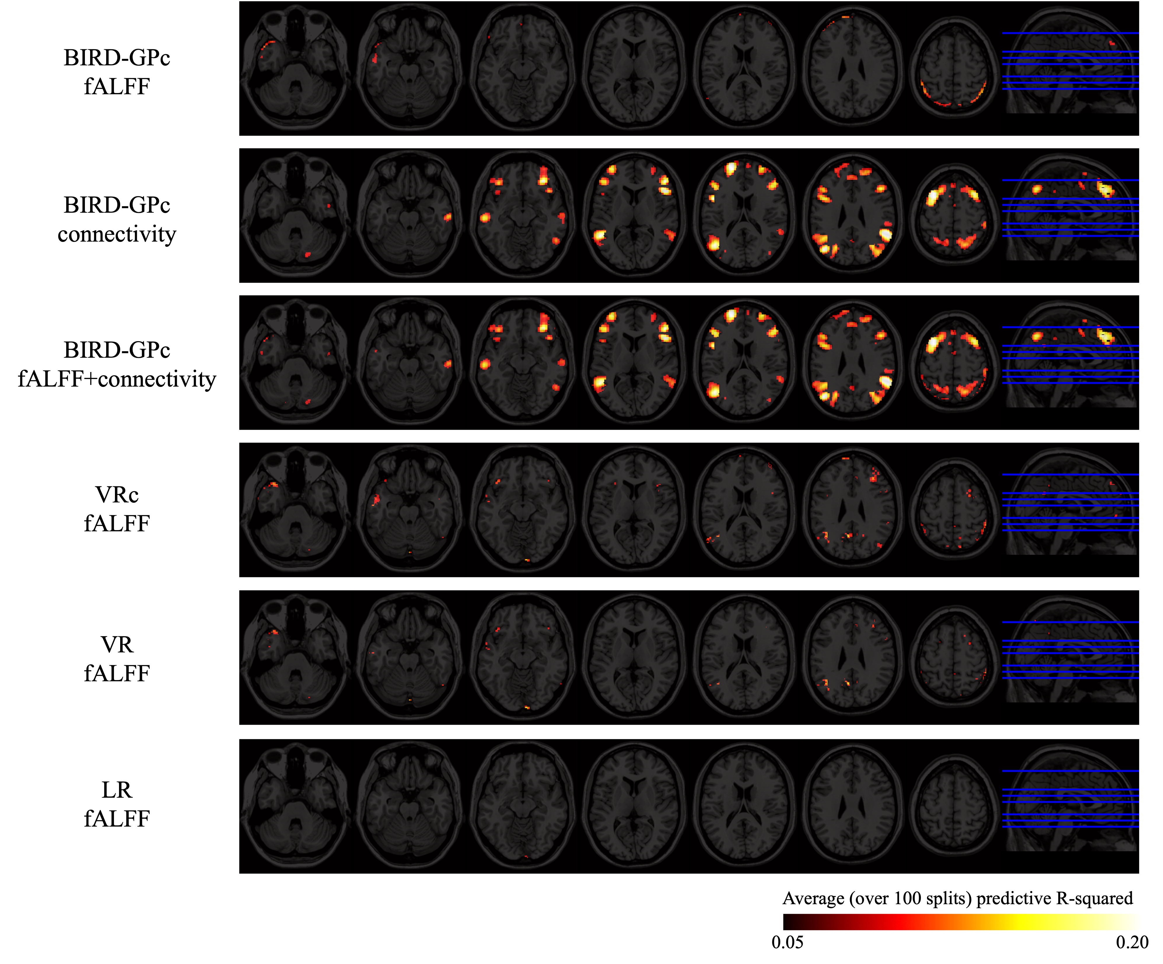
Figure 5: Language task: the voxel-wise average predictive $\bar{R^{2}}$ over the 100 train-test splits, by seven slices from the axial view ($z=40,50,60,80,90,100,130$). Only predictable voxels ($\bar{R^{2}}>0.05$) are colored according to its $\bar{R^{2}}$.

We consider three types of predictors for our method, all ajusted for counferders: fALFF alone (BIRD-GPc fALFF), connectivity alone (BIRD-GPc connectivity), and both fALFF and connectivity (BIRD-GPc fALFF+connectivity). We compare our methods with linear regression (Tavor et al.,, 2016) and voxel-wise regression (Dworkin et al.,, 2016). Both regression method require predictor and outcome should be from the same image space, thus can only admit fALFF as predictor. Moreover, there is no straightforward adaptation of the linear regression model to adjust for confounders. Therefore, we consider three competing models: linear regression with fALFF (LR), voxel-wise regression with fALFF (VR), and voxel-wise regression with fALFF and adjusting for confounders (VRc). Results are summarized by brain regions annotated by the 116 automated anatomical labeling (AAL) (Tzourio-Mazoyer et al.,, 2002). We split the 714 subjects into an 80% training set and a 20% testing set, which we repeat for 100 times. See Supplementary Materials S6 for training details.

We compute the predictive $R^{2}$ for each voxel to assess the performance of the models on the testing data. Due to the inherent complexity of brain activities, predicting voxel-level outcomes is highly challenging, resulting in a significant number of voxels and regions that are not predictable by any model. To consider a voxel as predictable with a model, we set a threshold of an average predictive $\bar{R^{2}}$ greater than 0.05 over 100 splits. First, in Table 2(c), we compare BIRD-GPc fALFF with three competing models that also utilize fALFF as a predictor. Since fALFF has limited prediction power, a substantial portion of voxels and regions are not predictable by any of the methods. Instead, we report the proportion of predictable voxels, along with the mean and interquartile range (IQR) of the average predictive $\bar{R^{2}}$ of predictable voxels over 100 splits for selected regions. These selected regions include those where at least 5% of voxels are predictable by two models or at least 20% are predictable by one model. For the language task, BIRD-GPc fALFF demonstrates comparable performance with VRc and outperforms VR and LR in the selected region Temporal Pole Middle Temporal Gyrus Right (Temporal_Pole_Mid_R). For the social recognition task (random), BIRD-GPc overall exhibits the best performance in the selected regions Superior Parietal Gyrus Right (Parietal_Sup_R) and Calcarine Fissure and Surrounding Cortex Left (Calcarine_L).

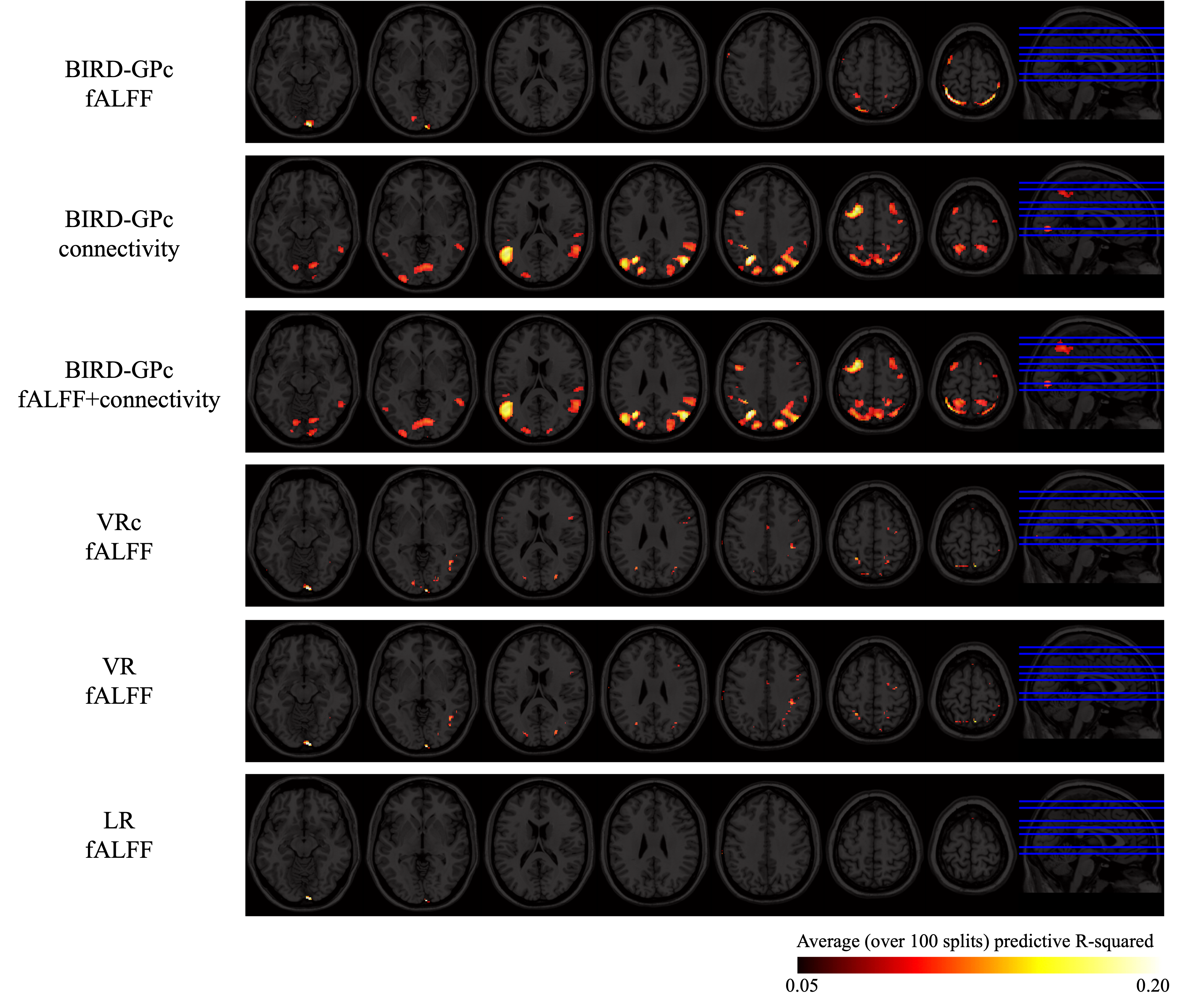
Figure 6: Social recognition task (random): the voxel-wise average predictive $\bar{R^{2}}$ over the 100 train-test splits, by seven slices from the axial view ($z=60,70,90,100,110,130,140$). Only predictable voxels ($\bar{R^{2}}>0.05$) are colored according to its $\bar{R^{2}}$.

We then compare BIRD-GP with three types of predictors in Table 3(c) and Table 4(c), for the two tasks respectively. For each task, we report the proportion of predictable voxels, the mean and (IQR) of the average predictive $\bar{R^{2}}$ over 100 splits of predictable voxels on the whole brain (All) and the top five most predictable regions by the proportion of in-region predictable voxels. BIRD-GP with both modalities has the highest proportion of predictable voxels in Angular Gyrus Right and Left (Angular_R and Angular_L), SupraMarginal Gyrus Left(SupraMarginal_L), Inferior Parietal Gyrus Left (Parietal_Inf_L) and Inferior Frontal Gyrus Triangular Part (Frontal_Inf_Tri_L) in the language task. In the social recognition task, BIRD-GP with both modalities has the highest proportion of predictable voxels in Superior Parietal Gyrus Right and Left (Parietal_Sup_R and Parietal_Sup_L), Superior Occipital Gyrus Right and Left (Occipital_Sup_R and Occipital_Sup_L), and Middle Occipital Gyrus Right (Occipital_Mid_R). We find that the language story-math contrast maps are more predictable by fALFF and connectivity than the social recognition random contrast maps. We also find that, for both tasks and adjusting for confounders, fALFF alone does not provide much predictability for both task contrast maps, while connectivity alone bear much more such predictability, and using both modalities yields the best prediction performance.

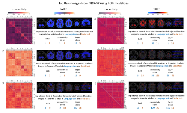
Figure 7: Six basis images associated with the most important dimensions of projected predictor images. These basis images are obtained from BIRD-GP using both fALFF and connectivity. We show the fALFF components by five slices from the axial view ($z=20,50,80,110,140$). We also list the importance ranks of their associated projected predictor image dimensions within separate models on both the language task and social recognition task (random).

We plot the voxel-wise average predictive $\bar{R^{2}}$ over the 100 train-test splits of predictable voxels by slices from the axial view in Figure 5 for the language task and Figure 6 for the social recognition task. Overall, BIRD-GP combining fALFF and connectivity (BIRD-GPc fALFF+connectivity) has the best performance. The three BIRD-GP models produce smoother prediction than VR and LR. In both tasks, our analysis reveals that BIRD-GP, when utilizing fALFF as the sole predictor, can predict well the boundary of regions Superior Parietal Gyrus (see the lower boundary of the last slice in the first row in Figure 5 and Figure 6). We confirm the predictability is not an artifact as detailed in Supplementary Materials S7. It is noteworthy that BIDR-GPc fALFF+connectivity is able to combine the advantage of BIRD-GP with fALFF alone (BIRD-GPc fALFF) and BIRD-GP with connectivity alone (BIRD-GPc connectivity). For example, for both tasks, BIRD-GPc fALFF can predict the bottom border well in the last slice while BIRD-GPc connectivity cannot. However, BIRD-GPc fALFF+connectivity combines the highlighted region of the two separate models.

5.3 Importance of the projected predictor image

We assess the importance of all dimensions of the projected predictor image in each of the three BIRD-GP models according to (5) and plot the basis images associated with most important dimensions. Figure 7 shows six basis images from BIRD-GPc fALFF+connectivty associated with the most important dimensions in the projected predictor image. We observe clear block patterns within functional modules in the connectivity component of basis images with high rankings. In Figure 7, for each presented basis image, we also show the importance ranks of the associated dimension of the projected predictor image. As basis images produced by the three BIRD-GP models are different, we perform basis images matching across models for presentation convenience. For each basis image from BIRD-GPc fALFF+connectivity, we identify a basis image from BIRD-GPc fALFF that exhibits the highest magnitude of correlation with the fALFF component of the basis image from BIRD-GPc fALFF+connectivity. Similarly, we match a basis image from BIRD-GPc connectivity that demonstrates the largest magnitude of correlation with the connectivity component.

In the language task, the projected predictor image dimensions associated with basis images 1, 2 and 3 are important in BIRD-GP using both modalities and BIRD-GP using connectivity alone. The projected predictor image dimension associated with basis image 4 is with high importance measure in BIRD-GP using both modalities and BIRD-GP with fALFF alone, but not important in BIRD-GP using connectivity alone. The projected predictor image dimension associated with basis image 5 is only important in BIRD-GP using both modalities, but that associated with basis image 6 is unimportant in all three models. In the social recognition tasks, the projected predictor image dimensions associated with basis images 1 and 2 are important in all three models, while those associated with basis images 3, 4 and 6 are only highly important in BIRD-GP using both modalities. The projected predictor image dimension associated with basis image 5 is not important in all three models.

6 Conclusion

This paper develops BIRD-GP for IIR by flexible modeling of complex associations between the predictor and outcome images via GP-based projections and DNN. Adopting the deep kernel learning strategy, BIRD-GP can efficiently construct the basis functions that capture the detailed characteristics of both the predictor and outcome images very well. Compared with other state-of-the-art methods, BIRD-GP can greatly reduce the number of model parameters, improve the prediction accuracy for IIR tasks and provide a set of basis images, leading to better interpretations of the model fitting. Our analysis of the HCP fMRI data by BIRD-GP reveals that the connectivity matrix has much more predictive power than fALFF on contrast maps from two HCP tasks, and combining both modalities achieve the best performance. We also identify the most predictable brain regions in both tasks by fALFF and the region-wise connectivity matrix.

References

- Binder et al., (2011) Binder, J. R., Gross, W. L., Allendorfer, J. B., Bonilha, L., Chapin, J., Edwards, J. C., Grabowski, T. J., Langfitt, J. T., Loring, D. W., Lowe, M. J., et al. (2011). Mapping anterior temporal lobe language areas with fMRI: a multicenter normative study. Neuroimage, 54(2):1465–1475.
- Carvalho et al., (2019) Carvalho, D. V., Pereira, E. M., and Cardoso, J. S. (2019). Machine learning interpretability: a survey on methods and metrics. Electronics (Switzerland), 8(8):1–34.
- Castelli et al., (2000) Castelli, F., Happé, F., Frith, U., and Frith, C. (2000). Movement and mind: a functional imaging study of perception and interpretation of complex intentional movement patterns. Neuroimage, 12(3):314–325.
- Dworkin et al., (2016) Dworkin, J. D., Sweeney, E. M., Schindler, M. K., Chahin, S., Reich, D. S., and Shinohara, R. T. (2016). Prevail: Predicting recovery through estimation and visualization of active and incident lesions. NeuroImage: Clinical, 12:293–299.
- Egorova et al., (2017) Egorova, N., Veldsman, M., Cumming, T., and Brodtmann, A. (2017). Fractional amplitude of low-frequency fluctuations (fALFF) in post-stroke depression. NeuroImage: Clinical, 16:116–124.
- Evans et al., (1993) Evans, A. C., Collins, D. L., Mills, S., Brown, E. D., Kelly, R. L., and Peters, T. M. (1993). 3D statistical neuroanatomical models from 305 MRI volumes. In 1993 IEEE Conference Record Nuclear Science Symposium and Medical Imaging Conference, pages 1813–1817. IEEE.
- Gelfand et al., (2003) Gelfand, A. E., Kim, H.-J., Sirmans, C., and Banerjee, S. (2003). Spatial modeling with spatially varying coefficient processes. Journal of the American Statistical Association, 98(462):387–396.
- Glasser et al., (2013) Glasser, M. F., Sotiropoulos, S. N., Wilson, J. A., Coalson, T. S., Fischl, B., Andersson, J. L., Xu, J., Jbabdi, S., Webster, M., Polimeni, J. R., et al. (2013). The minimal preprocessing pipelines for the human connectome project. Neuroimage, 80:105–124.
- Guo et al., (2022) Guo, C., Kang, J., and Johnson, T. D. (2022). A spatial Bayesian latent factor model for image-on-image regression. Biometrics, 78(1):72–84.
- Härkönen et al., (2020) Härkönen, E., Hertzmann, A., Lehtinen, J., and Paris, S. (2020). Ganspace: discovering interpretable GAN controls. In Advances in Neural Information Processing Systems, volume 33, pages 9841–9850.
- Harrewijn et al., (2020) Harrewijn, A., Abend, R., Linke, J., Brotman, M. A., Fox, N. A., Leibenluft, E., Winkler, A. M., and Pine, D. S. (2020). Combining fmri during resting state and an attention bias task in children. NeuroImage, 205:116301.
- Huang et al., (2018) Huang, H., Yu, P. S., and Wang, C. (2018). An introduction to image synthesis with generative adversarial nets. CoRR, abs/1803.04469.
- Isola et al., (2017) Isola, P., Zhu, J. Y., Zhou, T., and Efros, A. A. (2017). Image-to-image translation with conditional adversarial networks. In Proceedings - 30th IEEE Conference on Computer Vision and Pattern Recognition, CVPR 2017, volume 2017-Janua, pages 5967–5976.
- Kingma and Ba, (2015) Kingma, D. P. and Ba, J. (2015). Adam: a method for stochastic optimization. In International Conference on Learning Representations (ICLR).
- LeCun et al., (2010) LeCun, Y., Cortes, C., and Burges, C. (2010). MNIST handwritten digit database. ATT Labs [Online]. Available: http://yann.lecun.com/exdb/mnist.
- Lindquist, (2008) Lindquist, M. A. (2008). The Statistical Analysis of fMRI Data. Statistical Science, 23(4):439 – 464.
- Liu and Wang, (2016) Liu, Q. and Wang, D. (2016). Stein variational gradient descent: a general purpose Bayesian inference algorithm. In Lee, D., Sugiyama, M., Luxburg, U., Guyon, I., and Garnett, R., editors, Advances in Neural Information Processing Systems, volume 29. Curran Associates, Inc.
- Morris et al., (2011) Morris, J. S., Baladandayuthapani, V., Herrick, R. C., Sanna, P., and Gutstein, H. (2011). Automated analysis of quantitative image data using isomorphic functional mixed models, with application to proteomics data. The Annals of Applied Statistics, 5(2A):894.
- Power et al., (2011) Power, J. D., Cohen, A. L., Nelson, S. M., Wig, G. S., Barnes, K. A., Church, J. A., Vogel, A. C., Laumann, T. O., Miezin, F. M., Schlaggar, B. L., et al. (2011). Functional network organization of the human brain. Neuron, 72(4):665–678.
- Santhanam et al., (2017) Santhanam, V., Morariu, V. I., and Davis, L. S. (2017). Generalized deep image to image regression. In Proceedings of the IEEE Conference on Computer Vision and Pattern Recognition, pages 5609–5619.
- Sripada et al., (2019) Sripada, C., Angstadt, M., Rutherford, S., Kessler, D., Kim, Y., Yee, M., and Levina, E. (2019). Basic units of inter-individual variation in resting state connectomes. Scientific Reports, 9:1900–1911.
- Sripada et al., (2020) Sripada, C., Angstadt, M., Rutherford, S., Taxali, A., and Shedden, K. (2020). Toward a ”treadmill test” for cognition: improved prediction of general cognitive ability from the task activated brain. Human Brain Mapping, 41:3186–3197.
- Srivastava et al., (2014) Srivastava, N., Hinton, G., Krizhevsky, A., Sutskever, I., and Salakhutdinov, R. (2014). Dropout: a simple way to prevent neural networks from overfitting. The Journal of Machine Learning Research, 15(1):1929–1958.
- Tavor et al., (2016) Tavor, I., Jones, O. P., Mars, R., Smith, S., Behrens, T., and Jbabdi, S. (2016). Task-free MRI predicts individual differences in brain activity during task performance. Science, 352(6282):216–220.
- Tzourio-Mazoyer et al., (2002) Tzourio-Mazoyer, N., Landeau, B., Papathanassiou, D., Crivello, F., Etard, O., Delcroix, N., Mazoyer, B., and Joliot, M. (2002). Automated anatomical labeling of activations in SPM using a macroscopic anatomical parcellation of the MNI MRI single-subject brain. Neuroimage, 15(1):273–289.
- Van Essen et al., (2012) Van Essen, D. C., Ugurbil, K., Auerbach, E., Barch, D., Behrens, T. E., Bucholz, R., Chang, A., Chen, L., Corbetta, M., Curtiss, S. W., et al. (2012). The human connectome project: a data acquisition perspective. Neuroimage, 62(4):2222–2231.
- Wheatley et al., (2007) Wheatley, T., Milleville, S. C., and Martin, A. (2007). Understanding animate agents: distinct roles for the social network and mirror system. Psychological science, 18(6):469–474.
- WU-Minn HCP, (2017) WU-Minn HCP (2017). WU-Minn HCP 1200 subjects data release: Reference manual.
- Xiao et al., (2017) Xiao, H., Rasul, K., and Vollgraf, R. (2017). Fashion-MNIST: a novel image dataset for benchmarking machine learning algorithms. arXiv preprint arXiv:1708.07747.
- Zhang et al., (2018) Zhang, Q., Wu, Y. N., and Zhu, S. C. (2018). Interpretable convolutional neural networks. In Proceedings of the IEEE Computer Society Conference on Computer Vision and Pattern Recognition, pages 8827–8836.
- Zhao et al., (2015) Zhao, Y., Kang, J., and Long, Q. (2015). Bayesian multiresolution variable selection for ultra-high dimensional neuroimaging data. IEEE/ACM Transactions on Computational Biology and Bioinformatics, 15(2):537–550.
- Zou et al., (2008) Zou, Q.-H., Zhu, C.-Z., Yang, Y., Zuo, X.-N., Long, X.-Y., Cao, Q.-J., Wang, Y.-F., and Zang, Y.-F. (2008). An improved approach to detection of amplitude of low-frequency fluctuation (ALFF) for resting-state fMRI: fractional ALFF. Journal of Neuroscience Methods, 172(1):137–141.