On the tractability of Nash equilibrium

In this paper, we propose a method for solving a PPAD-complete problem (Papadimitriou, 1994). Given is the payoff matrix $C$ of a symmetric bimatrix game $(C,C^{T})$ and our goal is to compute a Nash equilibrium of $(C,C^{T})$. In this paper, we devise a nonlinear replicator dynamic (whose right-hand-side can be obtained by solving a pair of convex optimization problems) with the following property: Under any invertible $0\leq C\leq 1$, every orbit of our dynamic starting at an interior strategy of the standard simplex approaches a set of strategies of $(C,C^{T})$ such that, for each strategy in this set, a symmetric Nash equilibrium strategy can be computed by solving the aforementioned convex mathematical programs. We prove convergence using previous results in analysis (the analytic implicit function theorem), nonlinear optimization theory (duality theory, Berge’s maximum principle, and a theorem of Robinson (1980) on the Lipschitz continuity of parametric nonlinear programs), and dynamical systems theory (a theorem of Losert and Akin (1983) related to the LaSalle invariance principle that is stronger under a stronger assumption).

Introduction

Game theory is a mathematical discipline concerned with the study of algebraic, analytic, and other objects that abstract the physical world, especially social interactions. The most important solution concept in game theory is the Nash equilibrium (Nash, 1950), a strategy profile (combination of strategies) in an $N$-player game such that no unilateral player deviations are profitable. The Nash equilibrium is an attractive solution concept, for example, as Nash showed, an equilibrium is guaranteed to exist in any $N$-person game. Over time this concept has formed a basic cornerstone of economic theory, but its reach extends beyond economics to the natural sciences and biology.

In this paper, we propose a method, as an evolutionary dynamic (Sandholm, 2010), to compute a symmetric Nash equilibrium in a symmetric bimatrix game. This problem is PPAD-complete as follows from (Chen et al., 2009; Daskalakis et al., 2009) and a standard (folklore) symmetrization result of bimatrix games. We assume the payoff matrix to be invertible but this is only a mild assumption as singular matrices can be approximated arbitrarily well by invertible matrices. We do not attempt to ground the intuition of our equilibrium computation method from the perspective of economic theory. For example, proposing a microfoundation for our dynamic is beyond the scope of this paper. Methods for discretizing our equation are also out scope of our paper. We note that standard methods (such as the Euler or higher order methods such as Runge Kutta) certainly apply.

Preliminaries in game theory

Given a symmetric bimatrix game $(C,C^{T})$, we denote the corresponding standard (probability) simplex by $\mathbb{X}(C)$. $\mathbb{\mathring{X}}(C)$ denotes the relative interior of $\mathbb{X}(C)$. The elements (probability vectors) of $\mathbb{X}(C)$ are called strategies. We call the standard basis vectors in $\mathbb{R}^{n}$ pure strategies and denote them by $E_{i},i=1,\ldots,n$. Symmetric Nash equilibria are precisely those combinations of strategies $(X^{*},X^{*})$ such that $X^{*}$ satisfies $\forall Y\in\mathbb{X}(C):X^{*}\cdot CX^{*}-Y\cdot CX^{*}\geq 0$. We call $X^{*}$ a symmetric Nash equilibrium strategy. A symmetric Nash equilibrium is guaranteed to always exist (Nash, 1951). A simple fact is that $X^{*}$ is a symmetric Nash equilibrium strategy if and only if $(CX^{*})_{\max}-X^{*}\cdot CX^{*}=0$. If $(CX^{*})_{\max}-X^{*}\cdot CX^{*}\leq\epsilon$, $X^{*}$ is called an $\epsilon$-approximate equilibrium strategy. A symmetric bimatrix game $(C,C^{T})$ is zero-sum if $C$ is antisymmetric, that is, $C=-C^{T}$, and it is called doubly symmetric if $C$ is symmetric, that is, $C=C^{T}$. In this paper, we are concerned with a general $C$.

Definition 1.

$X$ is a fixed point of $(C,C^{T})$, if, for $i\in\{1,\ldots,n\}$, $X(i)>0\Rightarrow(CX)_{i}=X\cdot CX$.

Note that pure strategies and symmetric Nash equilibria are necessarily fixed points of $(C,C^{T})$.

Definition 2.

$X$ is an equalizer of $(C,C^{T})$, if, for all $Y\in\mathbb{X}(C)$, $X\cdot CX=Y\cdot CX$.

Note that an equalizer is necessarily a Nash equilibrium of $(C,C^{T})$.

Our techniques and main result

A plausible approach to compute a Nash equilibrium in this setting is to use the replicator dynamic

$$\dot{X}(i)=X(i)((CX)_{i}-X\cdot CX),\quad i=1,\ldots,n.$$

In this paper, we consider the more general dynamic

$$\dot{X}(i)=X(i)((CZ)_{i}-X\cdot CZ),\quad i=1,\ldots,n,$$

where $Z\in\mathbb{X}(C)$. We call parameter $Z$ the multiplier at $X$. Our main result has as follows:

Theorem 1.

Let $0\leq C\leq 1$ be the payoff matrix of a game $(C,C^{T})$ and let $S\equiv CC^{T}$. Then:

(i) Let $RE(\cdot,\cdot)$ denote the relative entropy function. For any $X\in\mathbb{X}(C)$, there exists $Z_{X}\in\mathbb{X}(C)$ as the unique minimizer of the convex optimization problem

minimize $$\theta_{X}RE(Z,X)+\frac{1}{2}\epsilon^{2}+\frac{1}{\alpha}\ln\left(\sum_{i=1}^{n}X(i)\exp\{\alpha(CZ)_{i}\}\right)-X\cdot CZ$$ (1)

subject to $$(X\cdot SX)^{-1}\sum_{i=1}^{n}X(i)(SX)_{i}(CZ)_{i}-X\cdot CZ\geq\epsilon\theta^{2}_{X}$$ (2)

$$\theta_{X}((CZ)_{\max}-X\cdot CZ)\leq\epsilon$$ (3)

$$Z\in\mathbb{X}(C),$$

where $\alpha>0$ is a constant and $\theta_{X}\geq 0$ is the unique optimizer of the also convex optimization problem

minimize $$RE(Z,X)-\theta$$ (4)

subject to $$(X\cdot SX)^{-1}\sum_{i=1}^{n}X(i)(SX)_{i}(CZ)_{i}-X\cdot CZ\geq\theta^{2}$$ (5)

$$Z\in\mathbb{X}(C).$$

(ii) If $C$ is invertible, starting at any $X^{0}\in\mathbb{\mathring{X}}(C)$, every limit point of the orbit $X_{t},t\in[0,+\infty)$ of

$$\dot{X}(i)=X(i)\left((CZ_{X})_{i}-X\cdot CZ_{X}\right),$$ (6)

where $Z_{X}$ is the multiplier that solves (1), as $t\rightarrow\infty$, is a strategy, say $X$, whose multiplier $Z_{X}$ is a symmetric Nash equilibrium strategy of $(C,C^{T})$.

Other related work

Our dynamic is a replicator dynamic, and, therefore, it is related to the multiplicative weights update method (Arora et al., 2012). The replicator dynamic and the multiplicative weights method have various applications in theoretical computer science, artificial intelligence, and game theory. On the latter front, there is significant amount of work on Nash equilibrium computation and especially in the setting of $2$-player games. We simply mention a boundary of those results. The Lemke-Howson algorithm for computing an equilibrium in a bimatrix game is considered by many to be the state of the art in exact equilibrium computation but it has been shown to run in exponential time in the worst case (Savani and von Stengel, 2004). There is a quasi-polynomial algorithm for additively approximate Nash equilibria in bimatrix games due to Lipton et al. (2003) (based on looking for equilibria of small support on a grid). Avramopoulos and Vasiloglou (2023) give a constructive existence proof of Nash equilibrium using the technique of multipliers (as we do in this paper). We note that the idea of using multipliers, in particular, in the related to this paper exponential multiplicative weights method, has independently been explored in (Piliouras et al., 2022; Avramopoulos, 2023). We also note that our method circumvents a tough impossibility result in game dynamics of Milionis et al. (2023). Insofar, the best polynomial-time approximation algorithm for a Nash equilibrium achieves a 0.3393 approximation (Tsaknakis and Spirakis, 2009).

Section 2 sketches the proof. Sections 3 and 4 set the stage and Section 5 proves our main result (Theorem 1). Section 6 presents a numerical experiment in a bad rock-paper-scissors game.

High-level proof sketch

The fixed points of (6) are those strategies $X\in\mathbb{X}(C)$ such that the right-hand-side of (6) is zero, that is, we have that

$$X(i)>0\Rightarrow(CZ_{X})_{i}=X\cdot CZ_{X}\quad i=1,\ldots,n.$$

We are going to provide two equivalent characterizations of the fixed points of (6) as either those strategies $X\in\mathbb{X}(C)$ such that

$$(X\cdot SX)^{-1}\sum_{i=1}^{n}X(i)(SX)_{i}(CZ_{X})_{i}-X\cdot CZ_{X}=0$$ (7)

or those strategies $X\in\mathbb{X}(C)$ such that

$$\epsilon_{X}\theta_{X}=0,$$ (8)

where $\epsilon_{X}$ is the optimizer of optimization problem (1). Note that, along a trajectory $X_{t},t\in[0,+\infty)$ of (6), we have that

$$\frac{d}{dt}X\cdot SX=\sum_{i=1}^{n}X(i)(SX)_{i}(CZ_{X})_{i}-(X\cdot SX)(X\cdot CZ_{X})$$

and, therefore, by constraints (2) and (3) (since $\epsilon\theta_{X}^{2}\geq 0$ where $\epsilon\geq 0$ is ensured by the latter constraint (3)), we obtain that, along a trajectory $X_{t},t\in[0,+\infty)$ of (6), we have that

$$\frac{d}{dt}X\cdot SX\geq 0.$$

Furthermore, by the previous characterization of fixed points in (7), the latter inequality is strict unless $X$ is a fixed point. Thus $X\cdot SX$ is a Lyapunov function for our dynamical system and a theorem of Losert and Akin (1983) implies that every limit point of the orbit our differential equation is a fixed point of (6). It remains to show that every limit point is a Nash equilibrium. To that end, note that by the previous characterization of fixed points in (8) we may only consider two cases, namely, either $\{\epsilon_{X}=0,\theta_{X}>0\}$ or $\{\theta_{X}=0\}$. In the former case, we show that the multiplier $Z_{X}$ is (always) a Nash equilibrium whereas, in the latter case, we show that if an orbit approaches such a fixed point, say, X, (one where $\theta_{X}=0$), from the interior, then the corresponding multiplier $Z_{X}$ is also a Nash equilibrium. Let us now delve directly into the proof:

On optimization problem (4)

Let us first briefly mention some properties of the relative entropy function. The relative entropy between the $n\times 1$ probability vectors $P>0$ (that is, for all $i=1,\ldots,n$, $P(i)>0$) and $Q>0$ is given by

$$RE(P,Q)\equiv\sum_{i=1}^{n}P(i)\ln\frac{P(i)}{Q(i)}.$$

However, this definition can be relaxed: Let $\mathcal{C}(\cdot)$ denote the carrier of its argument (that is always a probability vector), where the carrier is the set of indices with positive probability mass. The relative entropy between $n\times 1$ probability vectors $P$ and $Q$ where $Q\in\{\mathcal{Q}\in\mathbb{X}|\mathcal{C}(P)\subset\mathcal{C}(\mathcal{Q})\}$ and $\mathbb{X}$ is a probability simplex of appropriate dimension, is

$$RE(P,Q)\equiv\sum_{i\in\mathcal{C}(P)}P(i)\ln\frac{P(i)}{Q(i)}.$$

We note the well-known properties of the relative entropy (Weibull, 1995, p.96) that (i) $RE(P,Q)\geq 0$, (ii) $RE(P,Q)\geq\|P-Q\|^{2}$, where $\|\cdot\|$ is the Euclidean distance, (iii) $RE(P,P)=0$, and (iv) $RE(P,Q)=0$ iff $P=Q$. Note (i) follows from (ii) and (iv) follows from (ii) and (iii). Note finally that

$$\mathcal{C}(P)\not\subset\mathcal{C}(\mathcal{Q})\Rightarrow RE(P,Q)=\infty.$$

Lemma 1.

The following are properties of optimization problem (4):

(i) $\forall X\in\mathbb{X}(C)$, (4) is feasible.

(ii) At the optimal solution, say, $(\theta_{X},Y_{X})$, $RE(Y_{X},X)$ is bounded (finite).

(iii) $\forall X\in\mathbb{X}(C)$, $\theta_{X}\geq 0$, where the inequality is strict unless $X$ is a fixed point of $(S,S)$.

(iv) $\theta_{X}$ is an analytic function of $X$ except perhaps at fixed points of $(S,S)$.

Proof.

Let $\hat{C}$ be a square matrix of the same size as $C$ that agrees with $C$ on the subgame of $C$ corresponding to the carrier of $X$ and whose remaining entries are equal to zero. Furthermore, let $\hat{S}=\hat{C}\hat{C}^{T}$. Then letting

$$\hat{Y}=\left(\sum_{i=1}^{n}(\hat{C}^{T}X)_{i}\right)^{-1}\hat{C}^{T}X,$$

implying $\hat{Y}$ has the same carrier as $X$, we obtain that

$$(X\cdot\hat{S}X)^{-1}\sum_{i=1}^{n}X(i)(\hat{S}X)_{i}(\hat{C}\hat{Y})_{i}-X\cdot\hat{C}\hat{Y}=(X\cdot\hat{S}X)^{-1}\sum_{i=1}^{n}X(i)(\hat{S}X)_{i}(\hat{S}X)_{i}-X\cdot\hat{S}X$$

and, therefore, from Jensen’s inequality that

$$(X\cdot\hat{S}X)^{-1}\sum_{i=1}^{n}X(i)(\hat{S}X)_{i}(\hat{C}\hat{Y})_{i}-X\cdot\hat{C}\hat{Y}\geq 0,$$

and observing further, as follows from straight matrix algebra, that

$$(X\cdot SX)^{-1}\sum_{i=1}^{n}X(i)(SX)_{i}(C\hat{Y})_{i}-X\cdot C\hat{Y}=(X\cdot\hat{S}X)^{-1}\sum_{i=1}^{n}X(i)(\hat{S}X)_{i}(\hat{C}\hat{Y})_{i}-X\cdot\hat{C}\hat{Y},$$

we obtain that

$$(X\cdot SX)^{-1}\sum_{i=1}^{n}X(i)(SX)_{i}(C\hat{Y})_{i}-X\cdot C\hat{Y}\geq 0,$$ (9)

where the inequality is strict unless $X$ is a fixed point of $(S,S)$ (as follows from Jensen’s inequality). Therefore, $\forall X\in\mathbb{X}(C)$, (4) is feasible (since $\hat{Y}$ satisfies constraint (5)) as claimed in (i). Our proof of this claim also implies claim (ii) that $RE(Y_{X},X)$ is bounded (finite) since $\hat{Y}$, a feasible solution to the optimization problem, has a carrier that is a subset of the carrier of $X$ and, therefore $RE(\hat{Y},X)$ is finite (which implies that the optimal objective value of the optimization problem cannot be infinite and, therefore, the claim that $RE(Y_{X},X)$ must be finite). Let us now simultaneously prove (iii) and (iv): Taking the dual of (4), the Lagrangian is

$$\mathcal{L}(Z,\theta,\alpha,\lambda)=RE(Z,X)-\theta-\alpha\left((X\cdot SX)^{-1}\sum_{i=1}^{n}X(i)(SX)_{i}(CZ)_{i}-X\cdot CZ-\theta^{2}\right)+\lambda(\mathbf{1}^{T}Z-1),$$ (10)

where we assume that the constraints $Z\geq 0$ and $\theta\geq 0$ are implicit. The dual function $\mathcal{L}_{D}(\alpha,\lambda)$ is obtained by minimizing the Lagrangian $\mathcal{L}(Z,\theta,\alpha,\lambda)$, that is,

$$\mathcal{L}_{D}(\alpha,\lambda)=\inf\{\mathcal{L}(Z,\theta,\alpha,\lambda)|Z\in\mathbb{R}^{n},\theta\in\mathbb{R}\}.$$

The Lagrangian is minimized when the gradient is zero. Let us first set the partial derivative with respect to $\theta$ equal to zero to obtain

$$1-2\alpha\theta=0\Rightarrow\theta=\frac{1}{2\alpha},$$ (11)

which indeed satisfies $\theta\geq 0$ (therefore, proving the first part of (iii)) since $\alpha\geq 0$ (by the definition of the dual function), but (11) further implies that $\alpha>0$ and, therefore, $\theta>0$ unless $\alpha=\infty$. Let us now consider the partial derivative with respect to $Z$. Observing to that end that

$$\frac{\partial RE(Z,X)}{\partial Z(i)}=\frac{\partial}{\partial Z(i)}\left(Z(i)\ln\frac{Z(i)}{X(i)}\right)=1+\ln\frac{Z(i)}{X(i)}$$

we obtain that the gradient is zero when

$$1+\ln\frac{Z(i)}{X(i)}-\alpha\left((X\cdot SX)^{-1}\sum_{j=1}^{n}C^{T}_{ij}X(j)(SX)_{j}-(C^{T}X)_{i}\right)+\lambda=0.$$

Solving for $Z(i)$ in the previous expression, we obtain

$$Z(i)=X(i)\exp\left\{-1-\lambda+\alpha\left((X\cdot SX)^{-1}\sum_{j=1}^{n}C^{T}_{ij}X(j)(SX)_{j}-(C^{T}X)_{i}\right)\right\}\quad i=1,\ldots,n.$$ (12)

Note that, by the previous expression, the constraint $Z\geq 0$ is automatically satisfied. Using the notation

$$\mathcal{B}_{i}\equiv(X\cdot SX)^{-1}\sum_{j=1}^{n}C^{T}_{ij}X(j)(SX)_{j}-(C^{T}X)_{i},\quad i=1,\ldots,n,$$

and substituting now the previous expressions for $Z$ and $\theta$ in (10), we obtain the dual function

$$\mathcal{L}_{D}(\alpha,\lambda)= \sum_{i=1}^{n}X(i)\exp\{-1-\lambda+\alpha\mathcal{B}_{i}\}(-1-\lambda+\alpha\mathcal{B}_{i})-$$

$$-\alpha\sum_{i=1}^{n}X(i)\exp\{-1-\lambda+\alpha\mathcal{B}_{i}\}\mathcal{B}_{i}+$$

$$+\lambda\left(\sum_{i=1}^{n}X(i)\exp\{-1-\lambda+\alpha\mathcal{B}_{i}\}-1\right)+$$

$$-\frac{1}{2\alpha}+\alpha\left(\frac{1}{2\alpha}\right)^{2}$$

which simplifies to

$$\mathcal{L}_{D}(\alpha,\lambda)= -\sum_{i=1}^{n}X(i)\exp\{-1-\lambda+\alpha\mathcal{B}_{i}\}-\lambda-\frac{1}{4\alpha}.$$

This function is concave in $\alpha$ and $\lambda$. Since the dual function is concave, to find the optimal $\alpha$ and $\lambda$ we simply need to set the derivatives of $L_{D}(\alpha,\lambda)$ (with respect to $\alpha$ and $\lambda$) equal to $0$ (by the previous observation that $\alpha$ is necessarily strictly positive). To that end, we have

$$\frac{d\mathcal{L}_{D}(\alpha,\lambda)}{d\lambda}=\sum_{i=1}^{n}X(i)\exp\{-1-\lambda+\alpha\mathcal{B}_{i}\}-1=0,$$

which implies

$$\exp\{-1-\lambda\}=\frac{1}{\sum_{i=1}^{n}X(i)\exp\{\alpha\mathcal{B}_{i}\}}.$$

Substituting in (12) we obtain (by the zero duality gap since the problem is convex) the optimal $Z_{X}$ as

$$Z_{X}(i)=X(i)\frac{\exp\{\alpha\mathcal{B}_{i}\}}{\sum_{i=1}^{n}X(i)\exp\{\alpha\mathcal{B}_{i}\}}\quad i=1,\ldots,n.$$ (13)

Taking now the derivative of $L_{D}(\alpha,\lambda)$ with respect to $\alpha$ and setting it equal to zero, we obtain that

$$-\sum_{i=1}^{n}X(i)\mathcal{B}_{i}\frac{\exp\{\alpha\mathcal{B}_{i}\}}{\sum_{i=1}^{n}X(i)\exp\{\alpha\mathcal{B}_{i}\}}+\frac{1}{4\alpha^{2}}=0$$ (14)

(14) defines an implicit function. Note now that, by straight calculus and Jensen’s inequality, we have

$$\frac{d}{d\alpha}\left(\sum_{i=1}^{n}X(i)\mathcal{B}_{i}\frac{\exp\{\alpha\mathcal{B}_{i}\}}{\sum_{i=1}^{n}X(i)\exp\{\alpha\mathcal{B}_{i}\}}\right)\geq 0.$$

Let us show these steps: We have

$$\frac{d}{d\alpha}\left(\frac{\sum_{i=1}^{n}X(i)\mathcal{B}_{i}\exp\{\alpha\mathcal{B}_{i}\}}{\sum_{i=1}^{n}X(i)\exp\{\alpha\mathcal{B}_{i}\}}\right) =\frac{\left(\sum_{i=1}^{n}X(i)\mathcal{B}^{2}_{i}\exp\{\alpha\mathcal{B}_{i}\}\right)\left(\sum_{i=1}^{n}X(i)\exp\{\alpha\mathcal{B}_{i}\}\right)}{\left(\sum_{i=1}^{n}X(i)\exp\{\alpha\mathcal{B}_{i}\}\right)^{2}}-$$

$$-\frac{\left(\sum_{i=1}^{n}X(i)\mathcal{B}_{i}\exp\{\alpha\mathcal{B}_{i}\}\right)^{2}}{\left(\sum_{i=1}^{n}X(i)\exp\{\alpha\mathcal{B}_{i}\}\right)^{2}}$$

which is positive since, by Jensen’s inequality, we have

$$\frac{\sum_{i=1}^{n}X(i)\mathcal{B}^{2}_{i}\exp\{\alpha\mathcal{B}_{i}\}}{\sum_{i=1}^{n}X(i)\exp\{\alpha\mathcal{B}_{i}\}}\geq\left(\frac{\sum_{i=1}^{n}X(i)\mathcal{B}_{i}\exp\{\alpha\mathcal{B}_{i}\}}{\sum_{i=1}^{n}X(i)\exp\{\alpha\mathcal{B}_{i}\}}\right)^{2}$$

which implies that

$$\left(\sum_{i=1}^{n}X(i)\mathcal{B}^{2}_{i}\exp\{\alpha\mathcal{B}_{i}\}\right)\left(\sum_{i=1}^{n}X(i)\exp\{\alpha\mathcal{B}_{i}\}\right)\geq\left(\sum_{i=1}^{n}X(i)\mathcal{B}_{i}\exp\{\alpha\mathcal{B}_{i}\}\right)^{2}.$$

Therefore, the derivative (Jacobian) of (14) with respect to $\alpha$ is always $<0$ provided $\alpha$ is finite. Therefore, the $\mathcal{C}^{\infty}$ (analytic) implicit function theorem implies that for finite $\alpha>0$, and, therefore, also $\theta>0$ (by (11)), $\theta_{X}$ is an analytic function of $X$. In the rest of this proof, we show that the solution of our optimization problem (4) is obtained at $\alpha=\infty$ only if $X$ is a fixed point of $(S,S)$. To see what happens when $\alpha=\infty$, we may write (13) as

$$Z_{X}(i)=X(i)\frac{1}{\sum_{j=1}^{n}X(j)\exp\{\alpha(\mathcal{B}_{j}-\mathcal{B}_{i})\}}\quad i=1,\ldots,n$$

Taking the limit as $\alpha\rightarrow\infty$, we obtain that

$$\mathcal{B}_{i}<\mathcal{B}_{\max}\Rightarrow Z_{X}(i)=0$$

which implies

$$Z_{X}(i)>0\Rightarrow\mathcal{B}_{i}=\mathcal{B}_{\max}.$$

Therefore, by straight algebra, the optimal $Z_{X}$ is obtained at $\alpha=\infty$ only if

$$Z_{X}\in \arg\max\left\{\sum_{i=1}^{n}Z(i)\mathcal{B}_{i}\bigg{|}Z\in\mathbb{X}(C)\right\}=$$

$$=\arg\max\left\{(X\cdot SX)^{-1}\sum_{i=1}^{n}X(i)(SX)_{i}(CZ)_{i}-X\cdot CZ\bigg{|}Z\in\mathbb{X}(C)\right\}.$$

Note now that

$$\max\left\{(X\cdot SX)^{-1}\sum_{i=1}^{n}X(i)(SX)_{i}(CZ)_{i}-X\cdot CZ\bigg{|}Z\in\mathbb{X}(C)\right\}\geq 0$$ (15)

and the inequality is strict unless $X$ is a fixed point of $(S,S)$ (because (9) is strict unless $X$ is a fixed point of $(S,S)$). But $\alpha=\infty$ implies $\theta_{X}=0$ and, therefore, (15) cannot be strict. Therefore, (15) must be an equality and, thus, $X$ must be a fixed point of $(S,S)$. This completes the proof of (iii) and (iv). The proof of our lemma is thus complete. ∎

Lemma 2.

Let $\Gamma:\mathbb{X}(C)\rightrightarrows\mathbb{X}(C)\times[0,1]$ be the correspondence mapping an $X\in\mathbb{X}(C)$ to the set of $Z$ and $\theta$ that are feasible for the optimization problem (4). Then $\Gamma$ is a continuous correspondence.

Proof.

Following (Ok, 2007), to show $\Gamma$ is continuous it suffices to show that it is both upper-hemicontinuous and lower-hemicontinuous. Since $\mathbb{X}(C)$ is compact and the $\theta$ where (5) is feasible is also a compact set (since $\theta$ is necessarily upper and lower bounded), it is simple to show that $\Gamma$ is upper-hemicontinuous by simply invoking a characterization of upper-hemicontinuity as in (Ok, 2007, Proposition 2, p. 290) and following the rationale in (Ok, 2007, Example 2, p. 292) (giving a similar upper-hemicontinuity proof based on the Heine-Borel theorem that in compact sets every sequence has a convergent subsequence). To show it is lower-hemicontinuous we invoke the definition of lower hemi-continuity (Ok, 2007, p. 298) following (Ok, 2007, Example 3, p. 299).

Let us show these steps: Recall first that a correspondence $G:\mathbb{X}\rightrightarrows\mathbb{Y}$ between subsets of Euclidean space is said to be lower hemicontinuous at $X\in\mathbb{X}$ if, for every open set $O$ in $\mathbb{Y}$ with $G(X)\cap O\neq\emptyset$, there exists a $\delta>0$ such that

$$\forall X^{\prime}\in N_{\delta,\mathbb{X}}(X):G(X^{\prime})\cap O\neq\emptyset,$$

where $N_{\delta,\mathbb{X}}(X)=\{x\in\mathbb{X}:d(X,x)<\delta\}$ and $d(\cdot)=\|\cdot\|$, that is Euclidean distance. With this definition in place let us come back to our proof. Note that $\theta^{2}\geq 0$. If $X$ is a fixed point of $(S,S)$ such that $\theta=0$ is the only feasible value for the variable $\theta$, then $Z=X$ is the only feasible value for $Z$ and, therefore, since $\Gamma$ is upper-hemicontinuous, it is continuous at $X$. So let us assume that $X$ is such that some $\theta^{2}>0$ is feasible. For any such $X$ there exists $Z$ and $\theta$ such that the constraint (5) is a strict inequality. Take any open subset $O$ of $\mathbb{X}(C)$ with $\Gamma(X)\cap O\neq\emptyset$. To arrive at a contradiction, suppose that for every positive integer $m$ there exists an $X^{m}$ within $1/m$-neighborhood of $X$ such that $\Gamma(X^{m})\cap O=\emptyset$. Now pick any $(Z,\theta)\in\Gamma(X)\cap O$. Since $O$ is open in $\mathbb{X}(C)$, we have $((1-\lambda)Z_{0}+\lambda Z\in\Gamma(X),(1-\lambda)+\lambda\theta)\cap O$ for $\lambda\in(0,1)$ close enough to $1$, where $Z_{0}$ is the uniform strategy. But since $X^{m}\rightarrow X$, a straightforward continuity argument yields that constraint (5) is strictly satisfied for $m$ large enough. Then, for any such $m$, we have that $(1-\lambda)Z_{0}+\lambda Z\in\Gamma(X^{m})$, that is, $\Gamma(X^{m})\cap O\neq\emptyset$, a contradiction. Therefore, $\Gamma$ is lower-hemicontinuous, and, since it is upper-hemicontinuous, it is, thus, continuous. ∎

Lemma 3.

$\theta_{X}$ is a continuous function of $X\in\mathbb{X}(C)$.

Proof.

By Lemma 2, since the objective function of (1) is strictly convex, Berge’s maximum principle (Sundaram, 1996, p. 237) implies that $\theta_{X}$ is a continuous function of $X$. ∎

On optimization problem (1)

Lemma 4.

$\forall X\in\mathbb{X}(C)$ and $\forall\alpha>0$, we have that

$$\ln\left(\sum_{i=1}^{n}X(i)\exp\{\alpha(CZ)_{i}\}\right)$$

is a convex function of $Z$.

Proof.

It is well known that the logsumexp function

$$\ln\left(\sum_{i=1}^{n}\exp\{Z(i)\}\right)$$

is convex. It follows easily by a straightforward calculation of the Hessian that the function

$$f(Z)=\ln\left(\sum_{i=1}^{n}X(i)\exp\{Z(i)\}\right)$$

is also convex in $Z$. The lemma then follows by noting that $f(\alpha CZ)$ is also convex. ∎

Lemma 5.

$\forall X\in\mathbb{X}(C)$, (1) is feasible and bounded.

Proof.

Let $Y_{X}$ denote the optimal solution of (4). Lemma 1 implies that (1) is always feasible and bounded for $\epsilon=1$ since $Y_{X}$ is feasible. Note that since $Y_{X}$ is in the same carrier as $X$, $RE(Y_{X},X)$ is bounded. Therefore, the objective necessarily remains bounded at the optimal solution of (1). That $\epsilon=1$ always works for constraint (3) follows by the assumption that $0\leq C\leq 1$. ∎

Following Giorgi and Zucottti (2018), we consider a nonlinear program of the form

minimize $$\quad f(Z)$$

subject to $$\quad g_{i}(Z)\leq 0,i=1,\ldots,m$$

$$\quad h_{j}(Z)=0,j=1,\ldots,p,$$

where $f$, $g_{i},i=1,\ldots,m$, and $h_{j},j=1,\ldots,p$ are $\mathcal{C}^{2}$ (twice continuously differentiable). The Lagrangian associated with the previous problem is

$$\mathcal{L}(Z,u,w)=f(Z)+\sum_{i=1}^{m}u_{i}g_{i}(Z)+\sum_{j=1}^{p}w_{j}h_{j}(Z)$$

where $u=[u_{1},\ldots,u_{m}]^{T}$ and $w=[w_{1},\ldots,w_{p}]^{T}$ are the multiplier vectors.

Definition 3.

We say that the strong second order sufficient conditions hold at a feasible $Z$ with multipliers $(u,w)$ if

$$Y\cdot\nabla_{ZZ}^{2}\mathcal{L}(Z,u,w)Y>0$$

for all $Y\neq 0$ such that

$$\nabla g_{i}(Z)Y=0,\quad\mbox{ if }u_{i}>0$$

$$\nabla h_{j}(Z)Y=0,\quad j=1,\ldots,p.$$

Let us now consider the parametric nonlinear program

minimize $$\quad f(Z,X)$$

subject to $$\quad g_{i}(Z,X)\leq 0,i=1,\ldots,m$$

$$\quad h_{j}(Z,X)=0,j=1,\ldots,p,$$

where $f$, $g_{i},i=1,\ldots,m$, and $h_{j},j=1,\ldots,p$ are $\mathcal{C}^{2}$ in both $Z$ and $X$. Robinson (1980) (see also (Giorgi and Zucottti, 2018, Theorem 8)) shows that if $Z_{X}$, as a critical point of the aforementioned nonlinear program, satisfies the second order sufficient conditions, then $Z_{X}$ is a locally Lipschitz function of $X$.

Lemma 6.

For all $X\in\mathbb{X}(C)$ except perhaps at fixed points of $(S,S)$, the solution $Z_{X}$ of optimization problem (1) is a locally Lipschitz function of $X$.

Proof.

It follows from Lemma 1 (iv) that $\theta_{X}$ is an analytic function of $X$ except perhaps at fixed points of $(S,S)$. This implies that (1) then satisfies the requirement that the constraints are twice continuously differentiable. It only then remains to show that the second order sufficient condition is satisfied. To that end, note that we may identically express (1) as

minimize $$\theta_{X}RE(Z,X)+\frac{1}{2}\epsilon^{2}+\frac{1}{\alpha}\ln\left(\sum_{i=1}^{n}X(i)\exp\{\alpha(CZ)_{i}\}\right)-X\cdot CZ$$ (16)

subject to $$(X\cdot SX)^{-1}\sum_{i=1}^{n}X(i)(SX)_{i}(CZ)_{i}-X\cdot CZ\geq\epsilon\theta^{2}_{X}$$

$$\theta_{X}((CZ)_{i}-X\cdot CZ)\leq\epsilon,\quad i=1,\ldots,n$$

$$Z\in\mathbb{X}(C),$$

Let us form the Lagragian of (16) as

$$\mathcal{L}(Z,\epsilon,\lambda_{0},\lambda,\mu,\nu) =\theta_{X}RE(Z,X)+\frac{1}{2}\epsilon^{2}+\frac{1}{\alpha}\ln\left(\sum_{i=1}^{n}X(i)\exp\{\alpha(CZ)_{i}\}\right)-X\cdot CZ$$

$$+\lambda_{0}\left((X\cdot SX)^{-1}\sum_{i=1}^{n}X(i)(SX)_{i}(CZ)_{i}-X\cdot CZ-\epsilon\theta^{2}_{X}\right)$$

$$+\sum_{i=1}^{n}\lambda_{i}\left(\theta_{X}((CZ)_{i}-X\cdot CZ)-\epsilon\right)$$

$$-\mu_{1}Z(1)-\cdots-\mu_{n}Z(n)+\nu(Z(1)+\cdot+Z(n)-1).$$

Since every summand from the second to the fourth row of the previous Lagrangian expression is linear, we obtain that $\nabla^{2}_{\hat{Z}\hat{Z}}\mathcal{L}$, where $\hat{Z}=[Z^{T},\epsilon]^{T}$, is positive definite since, firstly, the relative entropy function is strictly convex (where is it is finite and the relative entropy is everywhere finite as follows from Lemma 5), secondly, the second derivative of $\frac{1}{2}\epsilon^{2}$ is equal to one, and, thirdly, by Lemma 4, the “logsumexp function” is convex. Therefore, the second order sufficiency condition is satisfied and we can apply (Robinson, 1980) ((Giorgi and Zucottti, 2018, Theorem 8)), which implies the lemma. ∎

Lemma 7.

$Z_{X}$ is a continuous function of $X\in\mathbb{X}(C)$.

Proof.

Observe that optimization problem (1) (of which $Z_{X}$ is the unique solution) is equivalent to the following optimization problem (where we are adding the explicit constraint $0\leq\epsilon\leq 1$ only as a matter convenience in our proof; that this constraint does not affect the solution of our optimization problem is implied by the assumption $0\leq C\leq 1$):

minimize $$\theta_{X}RE(Z,X)+\frac{1}{2}\epsilon^{2}+\frac{1}{\alpha}\ln\left(\sum_{i=1}^{n}X(i)\exp\{\alpha(CZ)_{i}\}\right)-X\cdot CZ$$ (17)

subject to $$(X\cdot SX)^{-1}\sum_{i=1}^{n}X(i)(SX)_{i}(CZ)_{i}-X\cdot CZ\geq\epsilon\theta^{2}_{X}$$ (18)

$$\theta_{X}((CZ)_{\max}-X\cdot CZ)\leq\epsilon,\quad i=1,\ldots,n$$ (19)

$$0\leq\epsilon\leq 1,\quad Z\in\mathbb{X}(C).$$

It, therefore, suffices to prove that the solutions of (17) vary continuously with $X$ (noting that, by Lemma 3, $\theta_{X}$ varies continuously with $X$). To that end, observe further that constraint (19) is always satisfied with strict inequality by slightly decreasing $\epsilon$ from the value $1$, which is always necessarily feasible, and that constraint (18) is always satisfied either strictly or vacuously by slightly decreasing $\epsilon$ from the value $1$ because $\theta_{X}$ is a solution to (4). The proof of our lemma follows then the same pattern as the proof of Lemmas 2 and 3. In particular, we consider the correspondence $\Gamma:\mathbb{X}(C)\rightrightarrows\mathbb{X}(C)\times[0,1]$, mapping an $X$ to the $Z$ and $\epsilon$ that are feasible for optimization problem (17). We first observe that because $Z$ and $\epsilon$ lie in a compact set, $\Gamma$ is necessarily upper-hemicontinuous (by compactness, every sequence has a convergent subsequence).

We then only need to prove that it is lower-hemicontinuous. The proof follows the same pattern as in Lemma 2: So let us assume that $Z$ and $\epsilon$ are such that (19) is satisfied with strict inequality. Take any open subset $O$ of $\mathbb{X}(C)\times[0,1]$ with $\Gamma(X)\cap O\neq\emptyset$. To obtain a contradiction, suppose that for every positive integer $m$ there exists an $X^{m}$ within $1/m$-neighborhood of $X$ such that $\Gamma(X^{m})\cap O=\emptyset$. Now pick any $(Z,\epsilon)\in\Gamma(X)\cap O$. Since $O$ is open in $\mathbb{X}(C)$, we have

$$(Z_{\lambda}\equiv(1-\lambda)Z_{0}+\lambda Z,(1-\lambda)+\lambda\epsilon)\in\Gamma(X)\cap O$$

for $\lambda\in(0,1)$ close enough to $1$, where $Z_{0}$ is the uniform strategy. But since $X^{m}\rightarrow X$ and $\theta_{X}$ is continuous in $X$, we obtain, regarding (18), that

$$(X^{m}\cdot SX^{m})^{-1}\sum_{i=1}^{n}X^{m}(i)(SX^{m})_{i}(CZ_{\lambda})_{i}-X^{m}\cdot CZ_{\lambda}\geq\epsilon\theta_{X}$$

(either strictly or vacuously), and, regarding (19), that

$$\theta_{X^{m}}((CZ_{\lambda})_{\max}-X^{m}\cdot CZ_{\lambda})<\epsilon$$

for $m$ large enough. Then, for any such $m$, we have that $Z_{\lambda}\in\Gamma(X^{m})$, that is, $\Gamma(X^{m})\cap O\neq\emptyset$, a contradiction. Therefore, $\Gamma$ is lower-hemicontinuous, and, since it is upper-hemicontinuous, it is, thus, continuous. Berge’s maximum principle implies then that $Z_{X}$ is indeed continuous in $X$. ∎

Proof of Theorem 1

Let us recall a result that is standard in the literature (for example, see (Weibull, 1995)), namely, that the Nash equilibria of doubly symmetric bimatrix game, say, $(S,S)$, coincide with the KKT points of the optimization problem

maximize $$\quad X\cdot SX$$

subject to $$\quad X\in\mathbb{X}(S).$$

Let us also recall that an interior fixed point of $(S,S)$ is necessarily a Nash equilibrium of $(S,S)$.

Lemma 8.

If $C$ is invertible, then $(S,S)$, where $S=CC^{T}$, has a finite number of fixed points.

Proof.

If $C$ is invertible, $S$ is positive definite ($X\cdot SX=X\cdot CC^{T}X=\|C^{T}X\|^{2}$) and, therefore, the quadratic form $X\cdot SX$ is strictly convex. Fixed points of $(S,S)$ that are not pure strategies are necessarily Nash equilibria of their carrier and, therefore, KKT points of their carrier. Let $X^{*}$ be a fixed point of $(S,S)$ that is not a pure strategy, let $\hat{S}$ be its carrier (i.e., the subgame for that individual face of the simplex), and let $\hat{X}^{*}$ be the restriction of $X^{*}$ to $\mathbb{X}(\hat{S})$. If $\hat{X}^{*}$ is a local maximum of its carrier, then (Bertsekas et al., 2003, Proposition 1.4.2) implies that $X\cdot\hat{S}X$ must be constant for all $X\in\mathbb{X}(\hat{S})$, which contradicts that $X\cdot SX$ is strictly convex. Therefore, since, by convexity, $\hat{X}^{*}$ cannot be a saddle point, it must be a global minimum of $X\cdot\hat{S}X$. Since the global minimizer of a strictly convex function is unique, $\hat{X}^{*}$ must be an isolated fixed point of $(\hat{S},\hat{S})$. Observe that this implies that $X^{*}$ must be an isolated fixed point of $(S,S)$ (for if it is not, there must exist some carrier whose fixed points are not isolated, which contradicts that $X\cdot SX$ is strictly convex). Since the fixed points of $(S,S)$ are necessarily isolated points and since a face (carrier) of the simplex cannot carry more than one isolated fixed points (not only in our convex case but also under any payoff matrix), the number of fixed points is also necessarily finite. ∎

Lemma 9.

If $X$ is a fixed point of $(S,S)$, where $S=CC^{T}$, then

$$\hat{Y}_{X}(i)=\left(\sum_{i=1}^{n}(\hat{C}^{T}\hat{X})_{i}\right)^{-1}\hat{C}^{T}\hat{X},$$

where $\hat{C}$ is payoff matrix of the subgame corresponding to the carrier of $X$ and $\hat{X}$ is the restriction of $X$ to its carrier, is an equalizer of $(\hat{C},\hat{C}^{T})$.

Proof.

Let $X$ be a fixed point of $(S,S)$ and let $\hat{S}$ be the payoff matrix of the subgame corresponding to the carrier of $X$. Furthermore, let $\hat{X}$ be the restriction of $X$ to $\mathbb{X}(\hat{S})$. Then $\hat{X}$ is an interior fixed point $(\hat{S},\hat{S})$, which implies that there exists $\mu>0$ such that

$$\hat{S}\hat{X}=\mu\mathbf{1}$$ (20)

where $\mathbf{1}$ is a vector of ones of appropriate dimension. We may equivalently write (20) as

$$\hat{C}\hat{C}^{T}\hat{X}=\mu\mathbf{1}.$$

Observing that

$$\hat{Y}_{X}=\left(\sum_{i=1}^{n}(\hat{C}^{T}\hat{X})_{i}\right)^{-1}\hat{C}^{T}\hat{X}$$

is a probability vector (strategy), the lemma follows by observing that there exists $\mu^{\prime}>0$ such that

$$\hat{C}\hat{Y}_{X}=\mu^{\prime}\mathbf{1}$$

which implies by straight algebra that, for all $\hat{Y}\in\mathbb{X}(\hat{C})$,

$$\hat{Y}_{X}\cdot\hat{C}\hat{Y}_{X}=\mu^{\prime}=\hat{Y}\cdot\hat{C}\hat{Y}_{X},$$

and, therefore, that $\hat{Y}_{X}$ is an equalizer of $(\hat{C},\hat{C}^{T})$ as claimed. ∎

Lemma 10.

(i) The fixed points (equilibria) of (6) are precisely those $X\in\mathbb{X}(C)$ where $\epsilon_{X}\theta_{X}=0$, where $\epsilon_{X}$ is the unique optimizer of (1) (and $\theta_{X}$ is the unique optimizer of (4)).

(ii) The fixed points (equilibria) of (6) are precisely those $X\in\mathbb{X}(C)$ where

$$(X\cdot SX)^{-1}\sum_{i=1}^{n}X(i)(SX)_{i}(CZ_{X})_{i}-X\cdot CZ_{X}=0.$$

(iii) Along an orbit of (6), we have that

$$\frac{d}{dt}X\cdot SX\geq 0.$$ (21)

Furthermore, unless $X\in\mathbb{X}(C)$ is a fixed point of (6), we have that (21) is a strict inequality.

Proof.

Note, as noted earlier, that $X$ is a fixed point of (6) if

$$X(i)>0\Rightarrow(CZ_{X})_{i}=X\cdot CZ_{X}.$$

Therefore, a necessary condition that $X$ is a fixed point of (6) is that

$$(X\cdot SX)^{-1}\sum_{i=1}^{n}X(i)(SX)_{i}(CZ_{X})_{i}-X\cdot CZ_{X}=0.$$

By constraint (2), a necessary condition that $X$ is a fixed point is, therefore, that $\epsilon_{X}\theta_{X}=0$. We, thus, need to show that it is also sufficient. If $\epsilon_{X}=0$ and $\theta_{X}>0$, then that $X$ is a fixed point of (6) is implied by constraint (3) which gives $(CZ_{X})_{\max}-X\cdot CZ_{X}=0$. If $\theta_{X}=0$, then, as implied by Lemma 1 (iii), $X$ is a fixed point of $(S,S)$. It remains to show that $X$ is also a fixed point of (6). To that end, note that optimization problem (1) reduces to

minimize $$\frac{1}{2}\epsilon^{2}+\frac{1}{\alpha}\ln\left(\sum_{i=1}^{n}X(i)\exp\{\alpha(CZ)_{i}\}\right)-X\cdot CZ$$

subject to $$Z\in\mathbb{X}(C),$$

which is equivalent to

minimize $$\frac{1}{\alpha}\ln\left(\sum_{i=1}^{n}X(i)\exp\{\alpha(CZ)_{i}\}\right)-X\cdot CZ$$

subject to $$Z\in\mathbb{X}(C).$$

Note now that, by Jensen’s inequality,

$$\frac{1}{\alpha}\ln\left(\sum_{i=1}^{n}X(i)\exp\{\alpha(CZ)_{i}\}\right)\geq X\cdot CZ$$

and the latter inequality is strict unless $X$ and $Z$ are such that

$$X(i)>0\Rightarrow(CZ)_{i}=X\cdot CZ.$$

This implies that the solution of our optimization problem is necessarily a fixed point of (6) provided such a fixed point exists. Let us show that it does: As in the proof of Lemma 1, let $\hat{C}$ be a square matrix of the same size as $C$ that agrees with $C$ on the subgame of $C$ corresponding to the carrier of $X$ and whose remaining entries are equal to zero. Furthermore, let $\hat{S}=\hat{C}\hat{C}^{T}$. Then letting

$$\hat{Y}=\left(\sum_{i=1}^{n}(\hat{C}^{T}X)_{i}\right)^{-1}\hat{C}^{T}X,$$

implying $\hat{Y}$ has the same carrier as $X$, we obtain that

$$\frac{1}{\alpha}\ln\left(\sum_{i=1}^{n}X(i)\exp\{\alpha(C\hat{Y})_{i}\}\right)-X\cdot C\hat{Y} =\frac{1}{\alpha}\ln\left(\sum_{i=1}^{n}X(i)\exp\{\alpha(\hat{C}\hat{Y})_{i}\}\right)-X\cdot\hat{C}\hat{Y}$$

$$=\frac{1}{\alpha}\ln\left(\sum_{i=1}^{n}X(i)\exp\{\alpha(\hat{S}X)_{i}\}\right)-X\cdot\hat{S}X$$

$$=0$$

where the last equality follows from Jensen’s inequality (the case for equality). Therefore, one possible solution of our optimization problem is $Z_{X}=\hat{Y}$ (since the objective value is then equal to zero whereas otherwise it is strictly positive) and to complete the proof that then $X$ is a fixed point of (6) note that

$$X(i)>0\Rightarrow(CZ_{X})_{i}=(C\hat{Y})_{i}=(SX)_{i}.$$ (22)

Therefore, since $X$ is a fixed point of $(S,S)$, that is,

$$X(i)>0\Rightarrow(SX)_{i}=X\cdot SX,$$

we obtain from (22) that

$$X(i)>0\Rightarrow(CZ_{X})_{i}=X\cdot CZ_{X}.$$

This completes the proof of (i).

As noted earlier in this proof, a necessary condition that $X$ is a fixed point of (6) is that

$$(X\cdot SX)^{-1}\sum_{i=1}^{n}X(i)(SX)_{i}(CZ_{X})_{i}-X\cdot CZ_{X}=0.$$ (23)

That (23) is also sufficient follows from the observation that, by constraint (2), (23) holds if and only if $\epsilon_{X}\theta_{X}=0$ and, therefore, (ii) follows from (i).

Note finally that

$$\frac{d}{dt}X\cdot SX=\sum_{i=1}^{n}X(i)(SX)_{i}(CZ_{X})_{i}-(X\cdot SX)(X\cdot CZ_{X}).$$

(21) follows then by constraint (2). That unless $X$ is a fixed point of (6), (21) is a strict inequality follows from (ii). This completes the proof of the lemma. ∎

We are almost ready now to use in our proof the following result, which strengthens the LaSalle invariance principle (for example, see (Khalil, 2002, p. 128)) under a stronger assumption.

Proposition 1 ((Losert and Akin, 1983)).

Suppose a continuous time dynamical system obtained from a differential equation on the simplex $\Delta$ admits a Lyapunov function $G:\Delta\rightarrow\mathbb{R}$, i.e., $\dot{G}(t)\geq 0$ with equality at the point $p$ of an orbit $p(t)$ only when $p$ is an equilibrium (fixed point) of the corresponding differential equation. The omega limit set of an orbit $p(t)$ is then a compact and connected set consisting entirely of equilibria (and upon which $G$ is constant).

In the next lemma, we use an argument nearly identical to that used in (Weibull, 1995, p. 119).

Lemma 11.

The interior $\mathbb{\mathring{X}}(C)$ of the simplex $\mathbb{X}(C)$ is invariant under (6).

Proof.

If $X^{0}\in\mathbb{\mathring{X}}(C)$ is a fixed point of $(S,S)$, then Lemma 1 implies that $\theta_{X^{0}}=0$ and then Lemma 10 implies that $X^{0}$ is also a fixed point of (6). Therefore, in this case, the interior $\mathbb{\mathring{X}}(C)$ is invariant under (6) as claimed. So let us assume $X^{0}\in\mathbb{\mathring{X}}(C)$ is not a fixed point of $(S,S)$ and denote by $X_{t}(X^{0}),t\geq 0$ the orbit of (6) starting at $X^{0}$. By Lemma 6 and the Picard-Lindelöf theorem, this orbit is unique. Note first that, since

$$\sum_{i=1}^{n}X(i)(CZ_{X}(i)-X\cdot CZ_{X})=0,$$

the orbit $X_{t}(X^{0}),t\geq 0$ lies on the tangent space of $\mathbb{X}(C)$. Let us assume for the sake of contradiction that there exists a time $\tau>0$ such that $X_{\tau}(X^{0})$ is a strategy on the boundary of $\mathbb{X}(C)$. This implies that there exists a pure strategy, say $i$, whose probability mass is equal to zero at time $\tau$. But the orbit of $X_{t}(X_{\tau}(X^{0}))$ is also (by Lemma 6 and the Picard-Lindelöf theorem) unique and it does not fall back in the interior of the simplex because of the multiplicative form of (6). ∎

Proof of Theorem 1.

Part (i) follows by Lemma 1 (i) and (ii) and also Lemma 5. Let us then prove (ii). We are going to consider two cases, namely, one where the initial condition $X^{0}$ is not a fixed point of $(S,S)$ and one where the initial condition is a fixed point of $(S,S)$.

Case 1: Lemmas 10 (iii) and 11 and Proposition 1 imply that, starting anywhere in the interior of $\mathbb{X}(C)$ (other than a fixed point of $(S,S)$), the omega limit set of the orbit of our equation is a compact and connected set consisting entirely of fixed points. Let us call this limit set $\mathbb{X}$. Let’s first assume that

$$\limsup\limits_{t\rightarrow\infty}\theta_{X_{t}}>0.$$ (24)

Let $X\in\mathbb{X}$ be such that $\theta_{X}>0$. Lemma 1 and (2) imply then that $\epsilon=0$ and, therefore, (3) implies that $(CZ_{X})_{\max}=X\cdot CZ_{X}$. Lemma 5 implies then that $RE(Z_{X},X)$ is finite, which further implies $X(i)=0\Rightarrow Z_{X}(i)=0$. But then, since $(CZ_{X})_{\max}=X\cdot CZ_{X}$ implies

$$X(i)>0\Rightarrow(CZ_{X})_{i}=(CZ_{X})_{\max},\quad i=1,\ldots,n$$

we obtain that

$$Z_{X}(i)>0\Rightarrow X(i)>0\Rightarrow(CZ_{X})_{i}=(CZ_{X})_{\max},\quad i=1,\ldots,n$$

and, therefore, that $(CZ_{X})_{\max}=Z_{X}\cdot CZ_{X}$. That is, $Z_{X}$ is a symmetric Nash equilibrium strategy.

Since the omega limit set of our equation is connected and, by Lemma 7, $Z_{X}$ is a continuous function of $X$, we obtain that the limit set of the orbit of multipliers is also connected. Therefore, (24) implies that $\mathbb{X}$ consists entirely of strategies whose multipliers are symmetric Nash equilibrium strategies (even if the $\liminf$ is zero) since equilibrium strategies cannot intersect non-equilibrium fixed points by the continuity of $(CZ_{X})_{\max}-Z_{X}\cdot CZ_{X}$.

Let’s now assume that

$$\limsup\limits_{t\rightarrow\infty}\theta_{X_{t}}=0.$$

By the assumption that $C$ is invertible, Lemma 8, that the limit set of our differential equation is connected, and Lemma 1 (iii), we obtain that $\mathbb{X}=\{X\}$, that is, a singleton fixed point of $(S,S)$. If $(CZ_{X})_{\max}=X\cdot CZ_{X}$, then, as before, $Z_{X}$ is a symmetric Nash equilibrium strategy. So let us assume that $(CZ_{X})_{\max}>X\cdot CZ_{X}$. Then, there must exist a pure strategy, say $i$, in the carrier of $X$ such that

$$(CZ_{X})_{i}>X\cdot CZ_{X}.$$ (25)

By the intermediate value theorem, there must exist a neighborhood $O$ of $X$ such that, for all $Y\in O\cap\mathbb{X}(C)$, we have that

$$(CZ_{Y})_{i}>Y\cdot CZ_{Y}.$$

Note that as follows from a straightforward calculation (for example, see (Weibull, 1995, pp. 98-100)), along $X_{t}$ we have that

$$\frac{d}{dt}RE(E_{i},X_{t})=X_{t}\cdot CZ_{X_{t}}-E_{i}\cdot CZ_{X_{t}}.$$

Within the neighborhood $O$ this derivative is strictly negative and the monotone convergence theorem implies that $RE(E_{i},X_{t})$ converges. But, since $X$ is a fixed point, we obtain that

$$\lim_{t\rightarrow\infty}\left\{\frac{d}{dt}RE(E_{i},X_{t})\right\}=0$$

which implies that

$$(CZ_{X})_{i}=X\cdot CZ_{X}$$

and contradicts (25). Therefore, it must be that $(CZ_{X})_{\max}=X\cdot CZ_{X}$, and, thus, $Z_{X}$ is a symmetric Nash equilibrium strategy (by the argument we have demonstrated).

Case 2: If the initial condition $X^{0}\equiv X$ is a fixed point of $(S,S)$, then, as implied by Lemma 1 (iii), $\theta_{X}=0$, and, therefore, $X$ is a fixed point of our differential equation (6). Furthermore, the proof of Lemma 10 (i) implies that $Z_{X}$ is equal to $\hat{Y}_{X}$ as that is given in the statement of Lemma 9. But then Lemma 9 implies that $Z_{X}=\hat{Y}_{X}$ is an equalizer of $(C,C^{T})$ and, therefore, a Nash equilibrium of $(C,C^{T})$. This completes the proof of Theorem 1. ∎

A numerical experiment

Optimization problems (1) and (4) are simple to implement in Matlab using the cvx convex optimization software (Grant and Boyd, 2014, 2008). Our numerical experiment is in a bad rock-paper-scissors game (for example, see (Sandholm, 2010)) where the standard replicator dynamic is known to spiral toward the boundary of the simplex (Riehl et al., 2018). We used the following bad rock-paper-scissors payoff matrix

$$C=\left[\begin{array}[]{ccc}0&-1&0.8\\ 0.8&0&-1\\ -1&0.8&0\\ \end{array}\right],$$

which we scaled by adding to every element $2$ and then dividing by $3$. In the objective function (1), we used $\alpha=10$. The initial condition was $(0.4,0.5,0.1)$. We discretized (6) using the following generalization of Hedge (Freund and Schapire, 1997, 1999):

$$X^{k+1}(i)=X^{k}(i)\frac{\exp\{\alpha(CZ_{X^{k}})_{i}\}}{\sum_{i=1}^{n}X^{k}(i)\exp\{\alpha(CZ_{X^{k}})_{i}\}},\quad i=1,\ldots,n$$

using learning rate $\alpha=1$. Figure 1 shows the relative entropy distance of the multipliers $Z_{X^{k}},k=0,\ldots,19$ from the Nash equilibrium of bad rock-paper-scissors which is the uniform strategy.

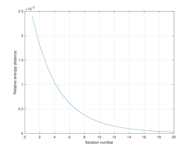
Figure 1: Relative entropy distance between the multipliers and the Nash equilibrium.

References

- Arora et al. [2012] S. Arora, E. Hazan, and S. Kale. The multiplicative weights update method: A meta-algorithm and its applications. Theory of Computing, 8:121–164, 2012.
- Avramopoulos [2023] I. Avramopoulos. Computational principles manifesting in learning symmetric equilibria by exponentiated dynamics. SSRN preprint https://ssrn.com/abstract=4425843, 2023.
- Avramopoulos and Vasiloglou [2023] I. Avramopoulos and N. Vasiloglou. On algorithmically boosting fixed-point computations. arXiv eprint 2304.04665 (cs.GT), 2023.
- Bertsekas et al. [2003] D. P. Bertsekas, A. Nedic, and A. E. Ozdaglar. Convex Analysis and Optimization. Athena Scientific, 2003.
- Chen et al. [2009] X. Chen, X. Deng, and S. Teng. Settling the complexity of computing two-player Nash equilibria. Journal of the ACM, 56(3), 2009.
- Daskalakis et al. [2009] C. Daskalakis, P. W. Goldberg, and C. H. Papadimitriou. The complexity of computing a Nash equilibrium. SIAM J. Comput., 39(1):195–259, 2009.
- Freund and Schapire [1997] Y. Freund and R. E. Schapire. A decision-theoretic generalization of on-line learning and an application to boosting. Journal of Computer and System Sciences, 55(1):119–139, 1997.
- Freund and Schapire [1999] Y. Freund and R. E. Schapire. Adaptive game playing using multiplicative weights. Games and Economic Behavior, 29:79–103, 1999.
- Giorgi and Zucottti [2018] G. Giorgi and C. Zucottti. A tutorial on sensitivity and stability in nonlinear programming and variational inequalities under differentiability assumptions. Dem working paper series #159 (06-18), Department of Economics and Management, University of Pavia, 2018.
- Grant and Boyd [2008] M. Grant and S. Boyd. Graph implementations for nonsmooth convex programs. In V. Blondel, S. Boyd, and H. Kimura, editors, Recent Advances in Learning and Control, Lecture Notes in Control and Information Sciences, pages 95–110. Springer-Verlag Limited, 2008. http://stanford.edu/~boyd/graph_dcp.html.
- Grant and Boyd [2014] M. Grant and S. Boyd. CVX: Matlab software for disciplined convex programming, version 2.1. http://cvxr.com/cvx, Mar. 2014.
- Khalil [2002] H. K. Khalil. Nonlinear Systems. Prentice Hall, third edition, 2002.
- Lipton et al. [2003] R. Lipton, E. Markakis, and A. Mehta. Playing large games using simple strategies. In Proc. EC’03, pages 36–41, 2003.
- Losert and Akin [1983] V. Losert and E. Akin. Dynamics of games and genes: Discrete versus continuous time. J. Math. Biology, 17:241–251, 1983.
- Milionis et al. [2023] J. Milionis, C. Papadimitriou, G. Piliouras, and K. Spendlove. An impossibility theorem in game dynamics. PNAS, 120(41), 2023.
- Nash [1950] J. F. Nash. Equilibrium points in -person games. PNAS, 36(1), Jan. 1950.
- Nash [1951] J. F. Nash. Non-cooperative games. The Annals of Mathematics, Second Series, 54(2):286–295, Sept. 1951.
- Ok [2007] E. Ok. Real analysis with economic applications. Princeton University Press, Princeton and Oxford, 2007.
- Papadimitriou [1994] C. H. Papadimitriou. On the complexity of the parity argument and other inefficient proofs of existence. Journal of Computer and System Sciences, 48(3):498–532, 1994.
- Piliouras et al. [2022] G. Piliouras, R. Sim, and S. Skoulakis. Beyond time-average convergence: Near-optimal uncoupled online learning via claivoyant multiplicative weights update. arXiv eprint 2111.14737 (cs.GT), 2022.
- Riehl et al. [2018] J. Riehl, P. Ramazi, and M. Cao. A survey on the analysis and control of evolutionary matrix games. Annual Reviews in Control, 45:87–106, 2018.
- Robinson [1980] S. M. Robinson. Strongly regular generalized equations. Mathematics of Operations Research, 5:43–62, 1980.
- Sandholm [2010] W. H. Sandholm. Population Games and Evolutionary Dynamics. MIT Press, 2010.
- Savani and von Stengel [2004] R. Savani and B. von Stengel. Exponentially many steps for finding a Nash equilibrium in a bimatrix game. In Proc. 45th Annual IEEE Symposium on Foundations of Computer Science, pages 258–267, 2004.
- Sundaram [1996] R. K. Sundaram. A First Course in Optimization Theory. Cambridge University Press, New York, 1996.
- Tsaknakis and Spirakis [2009] H. Tsaknakis and P. G. Spirakis. An optimization approach for approximate Nash equilibria. Internet Mathematics, 5(4):365–382, 2009.
- Weibull [1995] J. W. Weibull. Evolutionary Game Theory. MIT Press, 1995.