Gallai-Edmonds percolation of topologically protected collective Majorana excitations.

Abstract

Majorana networks, whose vertices represent localized Majorana modes and edges correspond to bilinear mixing amplitudes between them, provide a unified framework for describing the low energy physics of several interesting systems; examples include Kitaev magnets, SU(2) symmetric Majorana spin liquds, and proposed platforms for topological quantum computing using Majorana modes. Such networks are known to exhibit topologically protected collective Majorana modes if the combinatorial problem of maximum matchings (maximally-packed dimer covers) of the underlying graph has unmatched vertices (monomers), as is typically the case if the network is disordered. These collective Majorana modes live in “${\mathcal{R}}$-type regions” of the disordered graph, which host the unmatched vertices (monomers) in any maximum matching and can be identified using the graph theoretical Gallai-Edmonds decomposition. Here, we focus on vacancy disorder (site dilution) in general (nonbipartite) two dimensional lattices such as the triangular and Shastry-Sutherland lattices, and study the random geometry of such ${\mathcal{R}}$-type regions and their complements, i.e., “${\mathcal{P}}$-type regions” from which monomers are excluded in any maximum matching of the lattice. These ${\mathcal{R}}$-type and ${\mathcal{P}}$-type regions are found to display a sharply-defined Gallai-Edmonds percolation transition at a critical vacancy density $n_{v}^{\rm crit}$ that lies well within the geometrically percolated phase of the underlying disordered lattice. For $n_{v}<n_{v}^{\rm crit}$, ${\mathcal{R}}$-type regions percolate but there is a striking lack of self-averaging even in the thermodynamic limit, with the ensemble average being macroscopically different from the properties of individual samples: Each sample has exactly one infinite cluster, which is of type ${{\mathcal{R}}}$ (${\mathcal{P}}$) in a weakly $n_{v}$-dependent fraction $f<1$ ($1-f<1$) of the samples. Since the underlying disorder is uncorrelated and $f$ is neither 0 nor 1 in the thermodynamic limit throughout the low-$n_{v}$ phase, this unusual behavior may be viewed (from the perspective of the percolation of collective Majorana modes) as an apparent violation of the zero-one law that is typically expected to hold for percolation with uncorrelated disorder.

I Introduction

Several condensed matter systems are believed to host zero-energy Majorana modes which represent protected ground state degeneracies associated with defects or boundaries [1, 2, 3, 4, 5, 6, 7, 8]. Their presence is usually taken to be a signature of the non-trivial topology of the underlying many body ground state [9]. When there are many such Majorana modes, it is natural to model the resulting low energy physics in terms of a Majorana network [10, 11, 12, 13], with Hamiltonian

$$H_{\rm Majorana} = i\sum_{\langle rr^{\prime}\rangle}a_{rr^{\prime}}\eta_{r}\eta_{r^{\prime}}\;,$$ (1)

defined on a graph whose vertices $r$ host localized Majorana modes represented by Majorana operators $\eta_{r}$ and edges $\langle rr^{\prime}\rangle$ correspond to purely imaginary antisymmetric mixing amplitudes $ia_{rr^{\prime}}$ between these modes. In addition, this framework also captures the low-temperature physics of several interesting systems whose low-energy quasiparticle spectrum is captured exactly or well-approximated by a Hamiltonian of this type written in terms of Majorana fermion operators $\eta_{r}$. Examples of the latter include Kitaev magnets [14, 15, 16, 17, 18, 19, 20] and SU(2) symmetric Majorana spin liquds [21].

In the context of proposed platforms for topological quantum computing using such Majorana modes [22, 23, 24], the Majorana modes on the vertices of the network are the computational resource, and and the bilinear interactions associated with the edges of the network represent non-idealities that can degrade the performance of any protocol that aims to exploit these Majorana modes for computation. In the context of Kitaev magnets, there is an exact lattice-level mapping between the quantum magnet and the Majorana network [14, 15, 16, 17, 18, 19, 20]. In other examples, the connection is less explicit. For instance, for Majorana spin liquid states in general, the description in terms of a Majorana network relies on a parton description of the low energy physics of the Hamiltonian, and can include the effects of interactions between the Majorana fermions [21]. In all these contexts, the effects of quenched disorder are important at low energies and temperatures.

Do such networks as a whole exhibit collective zero-energy Majorana excitations that are robust to small perturbations of the network? The answer can have important implications. For instance, in the context of quantum computing, such collective Majorana modes could themselves potentially serve as a resource for quantum computing. Such collective Majorana modes are also associated with emergent local moments and low-temperature Curie tails in the susceptibility of SU(2) symmetric Majorana spin liquids [20].

Curiously enough, the apparently unconnected combinatorial problem of maximum matchings [25] or, equivalently, the classical statistical mechanics of the maximally-packed dimer model, provides a precise answer to this question [26]. In a matching, one matches vertices of a graph with a partner chosen from among its adjacent vertices, with the proviso that no two matched vertices share a partner. Equivalently, one places a dimer on some of the edges of the graph, with the proviso that no two dimers touch at a vertex. A maximum matching is then a matching with the fewest possible number of unmatched vertices, i.e. a maximally-packed dimer cover of the graph, with the least possible number of monomers.

a)

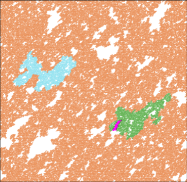
b)

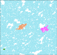
Figure 1: Snapshots of two different samples of the diluted triangular lattice, both with $L=5000$ and $n_{v}=0.48$. In each sample, the vertices belonging to the largest ${\mathcal{R}}$-type region are colored brown, those belonging to the second-largest ${\mathcal{R}}$-type region are colored bright pink, those belonging to the largest ${\mathcal{P}}$-type region are colored cyan, those belonging to the second-largest ${\mathcal{P}}$-type region are colored green, and those not belonging to any of these four clusters are left uncolored. a) The sample on the left has one very large ${\mathcal{R}}$-type region that appears to almost span the whole sample. In comparison, the largest two ${\mathcal{P}}$-type regions are both small. The second-largest ${\mathcal{R}}$-type region is even smaller. (b) The sample on the right has completely different morphology, with the largest ${\mathcal{P}}$-type region almost spanning the whole lattice, the largest and second-largest ${\mathcal{R}}$-type regions being rather small, and the second-largest ${\mathcal{P}}$-type region being the smallest of the four regions displayed. See Sec. IV.1 for details.

The statistical mechanics of such maximally-packed dimer models enters the picture as a result of the following observation: A Majorana network has collective topologically protected zero-energy Majorana excitations whenever the maximum matchings of the corresponding graph have unmatched vertices, as is typically the case if the graph is disordered [26, 27, 28]. Indeed, the number of linearly independent collective Majorana modes of this type is exactly equal to the number of monomers in any maximally packed dimer cover of the graph. Recent work [26] has also used the graph theoretical Gallai-Edmonds decomposition [29, 30, 25] to characterise the spatial profile of these collective Majorana modes by demonstrating that they live in so-called “${\mathcal{R}}$-type regions” of the disordered graph, which host the monomers of any maximally-packed dimer cover of the graph. This may be viewed as a generalization of the previously-established connection between topologically protected zero energy states in the spectrum of the tight-binding model on disordered bipartite lattices and such monomer-carrying ${\mathcal{R}}$-type regions of the lattice [31].

Here, we focus on vacancy disorder (site dilution) in general (nonbipartite) two dimensional lattices such as the triangular and Shastry-Sutherland lattices, and study the random geometry of such ${\mathcal{R}}$-type regions and their complements, i.e. “${\mathcal{P}}$-type regions” from which monomers are excluded in any maximum matching of the lattice. The results of our study reveal an interesting and unusual instance of a percolation phenomenon [32, 33, 34, 35]: We find that ${\mathcal{R}}$-type and ${\mathcal{P}}$-type regions have a sharply-defined Gallai-Edmonds percolation transition at a critical vacancy density $n_{v}^{\rm crit}$ that lies well within the geometrically percolated phase of the underlying disordered lattice. For $n_{v}<n_{v}^{\rm crit}$, there is a striking lack of self-averaging even in the thermodynamic limit: In a nonzero (weakly $n_{v}$-dependent) fraction $f<1$ of the samples, all ${\mathcal{P}}$-type regions are small and there is one infinite ${\mathcal{R}}$-type region. In the remaining fraction $1-f$ of the samples, all ${\mathcal{R}}$-type regions are small, and there is one infinite ${\mathcal{P}}$-type region.

Such percolation phenomena, that is, sharply defined phase transitions (as a function of the strength of the disorder) in the end-to-end connectivity of a random medium [32, 33, 34, 35], have been the focus of many decades of work in physics as well as in probability theory. It is therefore interesting to pause for a moment and ask where and how the Gallai-Edmonds percolation transition identified here fits into this body of knowledge. With this in mind, we use the remainder of this introductory discussion to provide some context for the striking behavior identified here.

Since the underlying quenched disorder is completely uncorrelated, it is tempting to view this lack of self-averaging from the vantage point of Bernoulli percolation, i.e. a phase transition in the end-to-end connectivity of a random medium in which the quenched disorder is completely uncorrelated in space. When viewed in this way, our percolated phase appears to violate the Kolmogorov zero-one law that applies to Bernoulli percolation, whereby the probability of having an infinite cluster in the thermodynamic limit cannot take on any value other than zero or one at any dilution [35, 36]. However, such an analogy misses an important feature of Gallai-Edmonds percolation: Although the disorder is indeed uncorrelated, the ${\mathcal{R}}$ or ${\mathcal{P}}$ labels of the vertices are certainly not uncorrelated. In fact, since these labels are determined by the structure of maximum matchings of the disodered lattice [25, 26], their correlations are related in a complicated way to the monomer and dimer correlation functions of the maximally-packed dimer model on the disordered lattice.

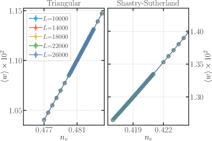
Figure 2: The sample-averaged density of monomers $w$ of the largest geometric cluster ${\mathcal{G}}$ of site-diluted triangular and Shastry-Sutherland lattices is nonzero in the thermodynamic limit. It decreases monotonically with decreasing dilution concentration $n_{v}$. See Sec. IV.1 for details.

a)

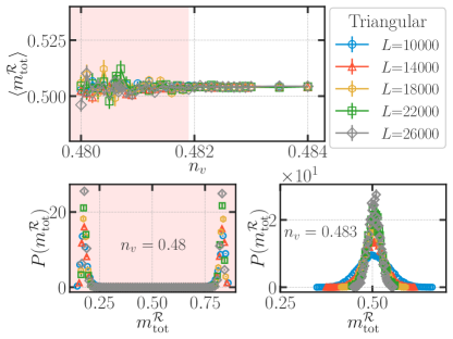
b)

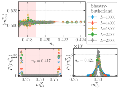
Figure 3: The sample-averaged total mass density of ${\mathcal{R}}$-type regions, ${m_{\rm tot}^{\mathcal{R}}}$, is nonzero and size-independent in the large $L$ limit. However, it develops large sample to sample fluctuations below a threshold value of $n_{v}$. (a) The figure on the left zooms in on this behavior in the vicinity of this threshold for the triangular lattice (b) The figure on the right zooms in on the corrresponding threshold for the Shastry-Sutherland lattice. The bottom panels of (a) and (b) display histograms that represent our numerical estimate of the corresponding probability distribution $P(m^{{\mathcal{R}}}_{\rm tot})$ at representative values of $n_{v}$ above and below this threshold. From these histograms, it is clear that the large sample to sample fluctuations seen below the threshold are actually caused by a bimodality in this probability distribution, as evidenced by two widely separated narrow peaks. This bimodality should be contrasted with the single peak seen above the threshold. See Sec. IV.1 for details.

Another instructive comparison is with Dulmage-Mendelsohn percolation [31], i.e. percolation of ${\mathcal{R}}$-type regions, constructed using Dulmage and Mendelsohn’s structure theory [25] for bipartite graphs, in site-diluted bipartite lattices. In this case, ${\mathcal{R}}$-type regions come in two flavours, ${\mathcal{R}}_{A}$-type regions in which all the monomers live only on $A$-sublattice sites of the lattice, and ${\mathcal{R}}_{B}$-type regions in which all the monomers live only on $B$-sublattice sites of the lattice. In two dimensions with site dilution, there seems to be no percolated phase. Instead, there is an incipient percolation transition of ${\mathcal{R}}$-type regions as $n_{v}\to 0$, causing their size to grow as $n_{v}^{-\nu}$ in this limit; here $\nu\approx 5.1$ is the universal correlation length exponent characterizing this incipient criticality.

a)

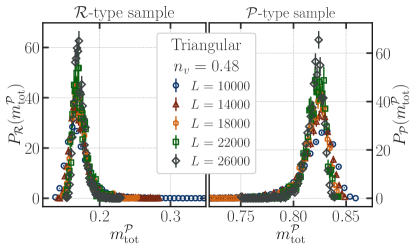
b)

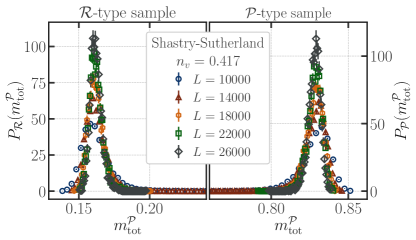
Figure 4: Each sample of (a) the site-diluted triangular lattice with $n_{v}=0.48$ (b) the Shastry-Sutherland lattice with $n_{v}=0.417$ is labeled ${\mathcal{R}}$-type or ${\mathcal{P}}$-type based on whether it contributes to the right peak or left peak respectively in the histogram of ${m_{\rm tot}^{\mathcal{R}}}$ in Fig. 3, where ${m_{\rm tot}^{\mathcal{R}}}$ is the total mass of ${\mathcal{R}}$ type regions in the largest geometric cluster ${\mathcal{G}}$ of the lattice scaled by the mass $m_{{\mathcal{G}}}$ of this geometric cluster. (a) For ${\mathcal{R}}$-type samples, the probability distribution $P_{{\mathcal{R}}}({m_{\rm tot}^{\mathcal{P}}})$ of ${m_{\rm tot}^{\mathcal{P}}}$, the total mass of ${\mathcal{P}}$-type regions in ${{\mathcal{G}}}$ scaled by $m_{{\mathcal{G}}}$, has a single peak at a small $L$-independent value of ${m_{\rm tot}^{\mathcal{P}}}$, (b) For ${\mathcal{P}}$-type samples, the probability distribution $P_{{\mathcal{P}}}({m_{\rm tot}^{\mathcal{P}}})$ of ${m_{\rm tot}^{\mathcal{P}}}$ has a single peak at a much larger $L$-independent value of ${m_{\rm tot}^{\mathcal{P}}}$. See Sec. IV.1 for details.

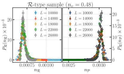
Triangular lattice a) b)

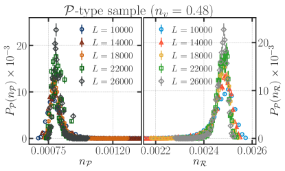
Figure 5: Each sample of the site-diluted triangular lattice with $n_{v}=0.48$ is labeled ${\mathcal{R}}$-type or ${\mathcal{P}}$-type based on whether it contributes to the right peak or left peak respectively in the histogram of ${m_{\rm tot}^{\mathcal{R}}}$ in Fig. 3, where ${m_{\rm tot}^{\mathcal{R}}}$ is the total mass of ${\mathcal{R}}$ type regions in the largest geometric cluster ${\mathcal{G}}$ of the lattice scaled by the mass $m_{{\mathcal{G}}}$ of this geometric cluster. (a) For ${\mathcal{R}}$-type samples, the probability distribution $P_{{\mathcal{R}}}({n_{\mathcal{R}}})$ of ${n_{\mathcal{R}}}$, the number of distinct ${\mathcal{R}}$-type regions scaled by the mass $m_{{\mathcal{G}}}$ of the largest geometric cluster, has a single peak at an $L$-independent small value of ${n_{\mathcal{R}}}$, while the probability distribution $P_{{\mathcal{R}}}({n_{\mathcal{P}}})$ of ${n_{\mathcal{P}}}$, the number of the distinct ${\mathcal{P}}$-type regions scaled by $m_{{\mathcal{G}}}$, has a single peak at a large $L$-independent value of ${n_{\mathcal{P}}}$. (b) For ${\mathcal{P}}$-type samples, the role of ${n_{\mathcal{P}}}$ and ${n_{\mathcal{R}}}$ is interchanged relative to ${\mathcal{R}}$-type samples. See Sec. IV.1 for details.

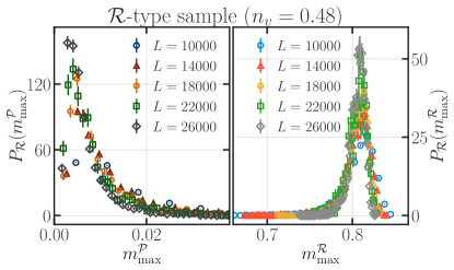
Triangular lattice a) b)

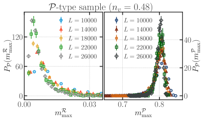
Figure 6: Each sample of the site-diluted triangular lattice with $n_{v}=0.48$ is labeled ${\mathcal{R}}$-type or ${\mathcal{P}}$-type based on whether it contributes to the right peak or left peak respectively in the histogram of ${m_{\rm tot}^{\mathcal{R}}}$ in Fig. 3, where ${m_{\rm tot}^{\mathcal{R}}}$ is the total mass of ${\mathcal{R}}$ type regions in the largest geometric cluster ${\mathcal{G}}$ of the lattice scaled by the mass $m_{{\mathcal{G}}}$ of this geometric cluster. (a) For ${\mathcal{R}}$-type samples, the probability distribution $P_{{\mathcal{R}}}({m_{\rm max}^{\mathcal{R}}})$ of ${m_{\rm max}^{\mathcal{R}}}$, the mass of the largest ${\mathcal{R}}$-type region scaled by the mass $m_{{\mathcal{G}}}$ of the largest geometric cluster, has a single peak at an $L$-independent large value of ${m_{\rm max}^{\mathcal{R}}}$, while the probability distribution $P_{{\mathcal{R}}}({m_{\rm max}^{\mathcal{P}}})$ of ${m_{\rm max}^{\mathcal{P}}}$, the mass of the largest ${\mathcal{P}}$-type region scaled by $m_{{\mathcal{G}}}$, has a single peak at a small value of ${m_{\rm max}^{\mathcal{P}}}$ which decreases with increasing $L$ (b) For ${\mathcal{P}}$-type samples, the behavior of ${m_{\rm max}^{\mathcal{P}}}$ and ${m_{\rm max}^{\mathcal{R}}}$ is interchanged relative to the behavior in ${\mathcal{R}}$-type samples. See Fig. 4 also. See Sec. IV.1 for details.

In contrast, on the three-dimensional cubic lattice, there are two percolated phases at successively lower values of $n_{v}$, with all ${\mathcal{P}}$-type clusters being small in both phases [31]. In the first of these phases, each sample has two infinite clusters in the thermodynamic limit, one ${\mathcal{R}}_{A}$-type and the other ${\mathcal{R}}_{B}$-type. In the second of these phases, each sample has only one infinite ${\mathcal{R}}$-type cluster in the thermodynamic limit, and this cluster spontaneously breaks the statistical bipartite symmetry of the random lattice by being either ${\mathcal{R}}_{A}$-type or ${\mathcal{R}}_{B}$-type with equal probability [31].

Thus, this phase also exhibits a lack of self-averaging. But this lack of self-averaging in the bipartite case is of a more familiar kind that is associated with all instances of spontaneous symmetry breaking in the thermodynamic limit, with the only slight subtlety being that the symmetry being spontaneously broken is a statistical bipartite symmetry of the ensemble of diluted lattices. Indeed, one can plausibly make an analogy between this phase and the Fortuin-Kastelyn cluster representation of the Z₂ symmetry broken low-temperature phase of the usual nearest neighbor ferromagnetic Ising model [37, 38, 39, 40, 41]. In this representation of the low temperature spontaneously magnetized phase, there is exactly one infinite cluster, but the spin label of this infinite cluster can be either $+1$ or $-1$. Clearly, the behavior identified here is qualitatively different from this, since there is no such symmetry between ${\mathcal{R}}$-type and ${\mathcal{P}}$-type clusters.

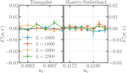
Figure 7: The ${\mathcal{R}}$-type or ${\mathcal{P}}$-type character of a particular sample is encoded in the value of the variable $\sigma$, with $\sigma=1$ for ${\mathcal{R}}$-type samples and $\sigma=0$ for ${\mathcal{P}}$-type samples. The parity of $m_{\mathcal{G}}$, i.e. whether the number of sites in the largest geometric cluster ${\mathcal{G}}$ is even or odd is encoded in the value of the variable $\tau$, with $\tau=0$ for even parity and $\tau=1$ for odd parity. The connected correlation function $C(\sigma,\tau)$, computed by averaging over 6000 to 20000 random samples (with a smaller number of samples for the largest size and vice versa) is shown in the figure. We see that our data is consistent with a vanishing $C(\sigma,\tau)$ (within our error bars), indicating that the ${\mathcal{R}}$-type or ${\mathcal{P}}$-type character of a sample is uncorrelated with the parity of $m_{\mathcal{G}}$. See Sec. IV.1 for details.

These comparisons with the usual expectations for Bernoulli percolation, the known behavior in the cluster representation of the usual nearest neighbor ferromagnetic Ising model, and with the behavior seen earlier in Dulmage-Mendelsohn percolation underscore the genuinely unusual nature of the Gallai-Edmonds percolation phenomena identified here. The rest of this article is devoted to a detailed account of these findings. In Sec. II, we review the Gallai-Edmonds theory and provide a summary of recent work [26] that uses this theory to identify regions of the graph that host topologically protected collective Majorana modes of the corresponding Majorana network Hamiltonian. Sec. IV is devoted to the results of our detailed computational study of the random geometry of ${\mathcal{R}}$-type and ${\mathcal{P}}$-type regions in site-diluted triangular and Shastry-Sutherland lattices. We conclude with a brief discussion of interesting directions for future work.

II Review: The Gallai-Edmonds theorem and collective Majorana modes

The structure theory of Gallai and Edmonds  [29, 30, 25], provides a characterization of any graph by exploiting invariant aspects of the structure of maximum matchings (maximally-packed dimer covers) of the graph. Here, we review this structure theory of general graphs, focusing only on those aspects with direct implications for the questions of interest to us. Following Ref. [26], we also review the decomposition of the graph into the ${\mathcal{R}}$-type and ${\mathcal{P}}$-type regions, and summarize earlier results on the significance of ${\mathcal{R}}$-regions for the identification of topologically-protected collective Majorana modes of Majorana networks.

a)

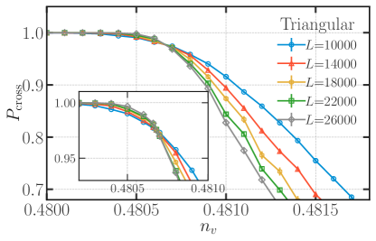
b)

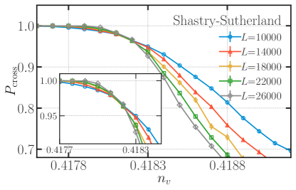
Figure 8: (a,b) $P_{\rm cross}$ is the probability that there exists a Gallai-Edmonds cluster (either a ${\mathcal{R}}$-type region or a ${\mathcal{P}}$-type region) in ${\mathcal{G}}$ (the largest geometrically connected component of the diluted lattice) which wraps around the torus in two independent directions. Our data reveals threshold behavior in $P_{\rm cross}$, with the threshold getting sharper with increasing system size. On the low-dilution side of this threshold, $P_{\rm cross}$ saturates to a size-independent value of $P_{\rm cross}\approx 1$. On the high-dilution side of this threshold, $P_{\rm cross}$ decreases monotonically with increasing size $L$. The inset zooms in on the vicinity of the threshold, and shows that curves corresponding to various sizes $L$ all cross at a critical dilution $n_{v}^{\rm crit}\approx 0.4807$ [$n_{v}^{\rm crit}\approx 0.4182$] on the triangular [Shastry-Sutherland] lattice. See Sec. IV.2 for details.

II.1 The Gallai-Edmonds decomposition

This theory, applicable to general graphs, provides a three-way classification of the vertices of the graph, into vertices labeled even (e-type), odd (o-type), and unreachable (u-type), along with a set of guarantees about the adjacency relations among these different types of vertices and a set of guarantees about which vertex types can be matched with each other in any maximum matching, and which vertices can remain unmatched in a maximum matching.

To obtain these labels, one has to first construct any one maximum matching, which can be done efficiently using the celebrated Edmonds’ “blossoms algorithm” [30]. These vertex labels can then be obtained using another iteration of the same Edmonds algorithm, starting with the maximum matching that has already been found. Their designations have to do with whether the vertex in question can be reached along an alternating path (with alternate edges not occupied by dimers and alternate edges occupied by dimers) starting from an unmatched vertex (monomer) of a maximum matching, and if they can be reached in this manner, whether they can be reached by some alternating path of even length starting from a monomer. Vertices which cannot be reached are labeled u-type, those that can be reached by an even-length alternating path labeled e-type, and all other vertices labeled o-type.

Primary among the useful guarantees provided by the Gallai-Edmonds theorem is the fact that this labeling does not depend on which maximum matching one starts with. In addition, it is guaranteed that e-type and u-type vertices cannot be adjacent to each other. Further, deletion of all edges between e-type and o-type vertices causes the e-type vertices to organize into distinct connected components, each of which contains an odd number of vertices. These odd-cardinality components are guaranteed to have a certain structure: they are built out of an odd cycle by attaching odd-length “ears” to it. In the remainder of this paper we slur over the (unimportant for our purposes) minor distinction between these odd-cardinality components and the “blossoms” that appear in most descriptions of Edmonds’ algorithm, and use “odd-cardinality components” and “blossoms” interchangeably to always refer to the connected components defined by the edge-deletion protocol given here.

In any maximum matching, u-type vertices are always matched to other u-type vertices, each o-type vertex is always matched with some other e-type vertex, and monomers of any maximum matching can only live on e-type vertices. Further, each odd-cardinality component (blossom) has exactly zero or one monomer on it in any maximum matching. Whether this monomer number is zero or one in any given maximum matching depends on whether an odd vertex is matched into the blossom or not. Further, given a blossom, one can always find a maximum matching that places a monomer on one of the vertices in that blossom

II.2 ${\mathcal{R}}$-type regions, ${\mathcal{P}}$-type regions, and collective Majorana modes

In Ref. [26], this structure theory of Gallai and Edmonds was used to establish the presence of a certain number of collective topologically protected Majorana modes of $H_{\rm Majorana}$ (Eq. 1) in specific regions of a disordered Majorana network; these regions were dubbed ${\mathcal{R}}$-type regions.

Their construction is straightforward: Delete all edges that connect any o-type vertex to any o-type or u-type vertices. The surviving edges only connect u-type vertices to each other, or e-type vertices to each other, or o-type vertices to e-type vertices. In the resulting graph, the e-type and o-type vertices form connected components; these are the ${\mathcal{R}}$-type regions of the original graph. Similarly, the u-type vertices form their own connected components; these define the ${\mathcal{P}}$-type regions of the original graph. In this way, the entire graph is decomposed into a set of non-overlapping (not sharing vertices) ${\mathcal{R}}$-type and ${\mathcal{P}}$-type regions.

Each ${\mathcal{R}}$-type region identified in this way is comprised of some number of odd-cardinality components (blossoms) $N_{\rm b}({\mathcal{R}})$ containing only e-type sites and links between them, and some number of o-type sites $N_{\rm o}({\mathcal{R}})$ to which these blossoms are connected (as noted earlier, there are no direct links between two odd-cardinality components). The Gallai-Edmonds theorem guarantees that the imbalance ${\mathcal{I}}({\mathcal{R}})\equiv N_{\rm b}({\mathcal{R}})-N_{\rm o}({\mathcal{R}})$ is positive for any ${\mathcal{R}}$-type region, and that the blossoms of each ${\mathcal{R}}$-type region host a total of exactly ${\mathcal{I}}({\mathcal{R}})$ monomers in any maximum matching of the graph, with each individual blossom hosting no more than one monomer. Thus, from the point of view of the maximum matchings of the graph, the ${\mathcal{R}}$-type regions are the monomer-carrying regions of the graph.

The basic result of Ref. [26] is that each such ${\mathcal{R}}$-type region hosts exactly ${\mathcal{I}}({\mathcal{R}})=N_{\rm b}({\mathcal{R}})-N_{\rm o}({\mathcal{R}})>0$ linearly independent collective topologically protected Majorana modes of the corresponding Majorana network. These modes have wavefunctions that are supported on all the e-type sites of the ${\mathcal{R}}$-type region. One way to see why this is the case is as follows: If we restrict the network Hamiltonian to an individual blossom, the matrix of mixing amplitudes is a pure imaginary antisymmetric matrix of odd dimension. Such a matrix generically must have one topologically protected zero eigenvector. Thus, each blossom, if disconnected from the rest of the graph, hosts one topologically protected collective Majorana mode. These will generically mix with each other and be destroyed when the nonzero mixing amplitudes connecting the blossoms to the odd vertices are reinstated. However, one can look for linear combinations that survive this mixing. To do this, one has to impose $N_{\rm o}({\mathcal{R}})$ constraints on $N_{\rm b}({\mathcal{R}})$, which allows ${\mathcal{I}}({\mathcal{R}})$ combinations to survive.

We close this discussion with a comment about a special case that has been studied earlier: When the Majorana network is bipartite, i.e. the graph corresponding to $H_{\rm Majorana}$ of Eq. 1 has a bipartition of vertices into two classes $A$ and $B$, such that vertices belonging to $A$ only have edges connecting them to vertices belonging to $B$ and vice-versa, the wavefunctions of topologically protected collective Majorana modes of the network can be constructed from the zero modes of an equivalent tight-binding Hamiltonian with purely real hopping amplitudes on the same graph.

Such topologically protected zero modes of bipartite hopping models also have an interesting description in graph theoretical terms, constructed using the Dulmage-Mendelsohn decomposition of bipartite graphs. This has been explored in some detail in previous work [31], and our results can be viewed as a natural generalization of these ideas to the case of general Majorana networks, with no bipartite restriction. From this point of view, our results in the triangular lattice case make for an interesting contrast with the previous results on the square lattice. For one may view the triangular lattice as a square lattice in which one has introduced additional nearest neighbor links corresponding to one set of diagonals. We discuss this further in Sec. IV.1

III Computational methods and observables

Motivated by the recent results reviewed in the previous section, we study the random geometry of Gallai-Edmonds clusters, i.e. ${\mathcal{R}}$-type and ${\mathcal{P}}$-type regions, of two-dimensional site-diluted lattices. The bulk of our numerical results are for $L\times L$ triangular and Shastry-Sutherland lattices with periodic boundary conditions and $L$ ranging from $L=10,000$ to $L=26000$ in both cases. The dilution is uncorrelated, and parameterized by a dilution fraction $n_{v}$ that represents the density of static (quenched) vacancies. Although our results are all within the geometrically percolated phase of the original lattice, the lattice itself can have several distinct connected components in some samples. To minimize finite-size effects, we focus attention on the largest connected component of the underlying diluted lattice, and study the random geometry of the Gallai-Edmonds decomposition of this component. We have typically averaged over three to ten thousand thousand such samples at each value of $n_{v}$ (with a smaller number of samples at the larger sizes). In addition to yielding accurate estimates of various self-averaging quantities, this also allows us to obtain reliable information about the probability distributions of quantities that have anomalously large sample-to-sample fluctuations.

For the diluted lattices under study, we find that a breadth-first search (BFS) based implementation of Edmonds’ matching algorithm performs better than a depth-first search (DFS) based implementation when we prune branches of the search tree to increase efficiency. We found that it is more efficient to start the search of augmenting paths with one monomer at a time rather than multiple monomers. Our BFS implementation relies on the version of Edmonds algorithm given by Moret and Shapiro [42] and uses the union-find data structure of Tarjan [43].In addition, we have also incorporated a few heuristics for the speed up of the matching algorithm; these are taken from the implementation published by Kececioglu and Pecqueur [44]. For instance, to increase the efficiency, an array of unmatched vertices is maintained at all times to help begin the search of augmenting paths.

Using this implementation of Edmonds’ algorithm, we proceed to obtain data along a grid of vacancy densities $n_{v}$ by using the maximum matching found earlier at an adjacent value of $n_{v}$ as the initial matching configuration for the algorithm. For the initial value of $n_{v}$ in our grid, a random matching was taken as an initial matching configuration. The data discussed in this paper was obtained by moving up in a grid of $n_{v}$ values.

After identifying a maximum matching of the lattice at a given vacancy concentration, we rerun the blossom algorithm to get the decomposition of sites into even, odd and unreachable sites. Then, starting from monomers, we build ${\mathcal{R}}$-type regions using a burning algorithm. After ${\mathcal{R}}$-type regions, ${\mathcal{P}}$-type regions are made using a similar burning algorithm. Once this is done at a given vacancy concentration, we move to the next higher vacancy concentration with existing matching as the initial condition. This process is then repeated to generate many random configurations to do the disorder averaging of the quantities, which we will describe next, measured during the burning of ${\mathcal{R}}$-type and ${\mathcal{P}}$-type regions.

As we have already reviewed, the physics of topologically protected collective Majorana modes is controlled by the size and morphology of the ${\mathcal{R}}$-type regions, and the structure of ${\mathcal{P}}$-type regions has no direct role in this physics. However, when it comes to understanding the interesting dilution dependence of the random geometry of these regions, it turns out to be useful to define and study both types of regions on an equal footing by keeping track of several different observables. We turn now to the definition of these observables.

Let ${\mathcal{G}}$ be the largest geometrically connected component of the lattice at a given dilution $n_{v}$ and $m_{{\mathcal{G}}}$ be its mass (number of sites). To minimize finite-size effects associated with small bits of the lattice split off from the largest connected component ${\mathcal{G}}$, we use the Gallai-Edmonds labeling of vertices of ${\mathcal{G}}$, and focus on its decomposition into a complete non-overlapping set of ${\mathcal{R}}$-type and ${\mathcal{P}}$-type regions.

For the simplest gross characterization of the structure of Gallai-Edmonds clusters, it is useful to study the $n_{v}$ dependence of the fraction of vertices of ${\mathcal{G}}$ that carry ${\mathcal{R}}$-type and ${\mathcal{P}}$-type labels. To this end, we define.

$${m_{\rm tot}^{\mathcal{R}}} = \frac{1}{m_{{\mathcal{G}}}}\sum_{{\mathcal{R}}_{i}\in{\mathcal{G}}}m_{{\mathcal{R}}_{i}}\;,$$

$${m_{\rm tot}^{\mathcal{P}}} = \frac{1}{m_{{\mathcal{G}}}}\sum_{{\mathcal{P}}_{i}\in{\mathcal{G}}}m_{{\mathcal{P}}_{i}}\;,$$ (2)

where the sum in the definition of ${m_{\rm tot}^{\mathcal{R}}}$ (${m_{\rm tot}^{\mathcal{P}}}$) is over ${\mathcal{R}}$-type (${\mathcal{P}}$-type) regions ${\mathcal{R}}_{i}$ (${\mathcal{P}}_{i}$) contained in ${\mathcal{G}}$, and $m_{{\mathcal{R}}_{i}}$ ($m_{{\mathcal{P}}_{i}}$) are their respective masses (total number of vertices contained in the cluster).

Another simple overall characterization is in terms of the total number $N_{{\mathcal{R}}}$ ($N_{{\mathcal{P}}}$) of ${\mathcal{R}}$-type (${\mathcal{P}}$-type) regions belonging to ${\mathcal{G}}$, and the total number $W$ of monomers in any maximum matching of ${\mathcal{G}}$. We define the corresponding number densities as

$$n_{{\mathcal{R}}} = N_{{\mathcal{R}}}/m_{{\mathcal{G}}}\;,$$

$$n_{{\mathcal{P}}} = N_{{\mathcal{P}}}/m_{{\mathcal{G}}}\;,$$

$$w = W/m_{{\mathcal{G}}}\;.$$ (3)

For a somewhat more detailed characterization of the structure of ${\mathcal{R}}$ and ${\mathcal{P}}$ type regions, we also keep track of their radius of gyration $R$. Since we work with periodic boundary conditions in both directions, this is tricky to measure efficiently unless defined in a suitable way. This issue has been discussed in the earlier literature, and we follow the definition and procedure suggested in Ref. [45]; this is also consistent with the approach used in an earlier study of the Dulmage-Mendelsohn percolation [31].

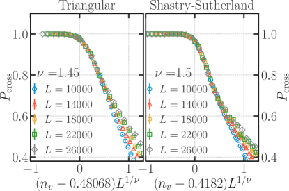
Figure 9: Data for $P_{\rm cross}(n_{v},L)$, the probability that there exists a GE cluster $\in{\mathcal{G}}$ that wraps around the torus in two independent directions for two dimensional $L\times L$ samples, for various $L$ and $n_{v}$ collapses onto a single scaling curve when plotted against the scaling variable $(n_{v}-n_{v}^{\rm crit})L^{1/\nu}$. See Sec. IV.2 for details

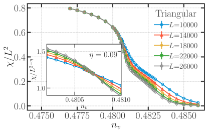
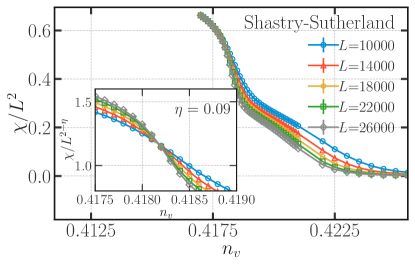
Figure 10: $\chi$, the susceptibility associated with sample-averaged geometric correlation function $C(r-r^{\prime})$ in $L\times L$ two dimensional samples, saturates to an $L$ independent value in the low-dilution phase. Data for $\chi(L,n_{v})$ when scaled by $L^{-\eta}$ crosses at $n_{v}^{\rm crit}$. See Sec. IV.2 for details.

In studies of geometric percolation, it is conventional to define a correlation function $C(r,r^{\prime})$ that takes on the value $C=1$ if $r$ and $r^{\prime}$ belong to the same cluster, and $C=0$ otherwise [33]. The corresponding correlation length $\xi$ is then related to the root mean square radius of gyration of the clusters, with each cluster of mass $m$ weighted by $m^{2}$ when calculating the mean [33]. With this in mind, we also define:

$$\xi^{2} = \left\langle\frac{\sum_{i\in{\mathcal{G}}}m_{i}^{2}R_{i}^{2}}{\sum_{i\in{\mathcal{G}}}m_{i}^{2}}\right\rangle\;,$$

$$\xi^{2}_{{\mathcal{R}}} = \left\langle\frac{\sum_{{\mathcal{R}}_{i}\in{\mathcal{G}}}m_{{\mathcal{R}}_{i}}^{2}R_{i}^{2}}{\sum_{{\mathcal{R}}_{i}\in{\mathcal{G}}}m_{{\mathcal{R}}_{i}}^{2}}\right\rangle\;,$$

$$\xi^{2}_{{\mathcal{P}}} = \left\langle\frac{\sum_{{\mathcal{P}}_{i}\in{\mathcal{G}}}m_{{\mathcal{P}}_{i}}^{2}R_{i}^{2}}{\sum_{{\mathcal{P}}_{i}\in{\mathcal{G}}}m_{{\mathcal{P}}_{i}}^{2}}\right\rangle\;.$$ (4)

Here, the sum over $i\in{\mathcal{G}}$ in the definition of $\xi$ is over all Gallai-Edmonds clusters (both ${\mathcal{P}}$-type and ${\mathcal{R}}$-type) belonging to the largest geometric cluster ${\mathcal{G}}$, while the corresponding sum in the definition of $\xi_{\mathcal{R}}$ ($\xi_{\mathcal{P}}$) is restricted to all ${\mathcal{R}}$-type (all ${\mathcal{P}}$-type) Gallai-Edmonds regions belonging to ${\mathcal{G}}$. The radius of gyration $R_{i}$ that appears in the above is again defined and measured as in Ref. [45]. As a result, these definitions of correlation lengths do not correspond exactly to the quantity one would have obtained from the correlation function $C(r,r^{\prime})$. However, when clusters are large, they behave in the same way, and the definition suggested in Ref. [45] is computationally much more efficient.

We also find it instructive to study the statistics of the largest ${\mathcal{R}}$-type and ${\mathcal{P}}$-type clusters in each sample by recording their radii of gyration $R^{{\mathcal{R}}}_{\rm max}$ and $R^{{\mathcal{P}}}_{\rm max}$, $\mathcal{I}_{\rm max}^{{\mathcal{R}}}$, the number of collective Majorana modes or monomers that live in the largest ${\mathcal{R}}$-type region, and $m^{{\mathcal{R}}}_{\rm max}$ and $m^{{\mathcal{P}}}_{\rm max}$, the masses of the largest ${\mathcal{R}}$ and ${\mathcal{P}}$ type regions in ${\mathcal{G}}$, the largest geometric cluster, scaled by $m_{\mathcal{G}}$, the mass of ${\mathcal{G}}$. In addition, we keep track of the susceptibility $\chi$ corresponding to the correlation function $C(r,r^{\prime})$:

$$\chi = \frac{1}{L^{2}}\sum_{r,r^{\prime}}\langle C(r,r^{\prime})\rangle$$ (5)

$$= \frac{1}{L^{2}}\left\langle\sum_{i\in{\mathcal{G}}}m_{i}^{2}\;.\right\rangle$$

Anticipating percolation-like behaviour of ${\mathcal{R}}$-type and ${\mathcal{P}}$-type regions, we have also measured various wrapping probabilities [46, 47, 48] that are sensitive to the presence of large clusters. The first of these is $P_{\rm cross}$, the probability that a sample has a Gallai-Edmonds cluster that (either ${\mathcal{R}}$-type or ${\mathcal{P}}$-type) wraps around the torus in two independent directions, i.e. a cluster characterized by two linearly independent winding vectors. The other quantity we keep track of is $P_{\rm single}$, the probability that a sample does not have any cluster that wraps around the torus in two independent directions, but does have a Gallai-Edmonds cluster that wraps around the periodic sample only in one direction.

IV Computational results

With these definitions in hand, we now present the results of our computational study of the structure of ${\mathcal{R}}$-type and ${\mathcal{P}}$-type regions in the largest geometrically connected component ${\mathcal{G}}$ of randomly site-diluted triangular lattice and Shastry-Sutherland lattices. In order to provide a clear description of the rather unusual behavior of these Gallai-Edmonds clusters, we focus in the main text on a minimal set of observables that lead us to unambiguous conclusions about the large-scale geometry, relegating many other pieces of supporting evidence to an appendix that can be consulted for further details.

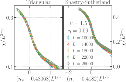
Figure 11: The susceptibility $\chi(L,n_{v})$, associated with the sample-averaged correlation function $C(r-r^{\prime})$ in $L\times L$ two dimensional samples, when scaled by $L^{2-\eta}$ and plotted against the scaling variable $(n_{v}-n_{v}^{\rm crit})L^{1/\nu}$, for appropriate choice of $\nu$ and $\eta$, collapses onto a single curve. See Sec. IV.2 for details.

IV.1 Thermodynamic densities

We start with the most basic question and ask if $w=\langle W/m_{\mathcal{G}}\rangle$ is finite in the thermodynamic limit of large linear size $L$, and if yes, how this monomer density changes with the dilution $n_{v}$ for the triangular and the Shastry-Sutherland lattice. We find that the ensemble average $\langle w\rangle$ over our ensemble of diluted samples is indeed nonzero in the thermodynamic limit, and appears to decrease smoothly with decreasing $n_{v}$. This is in some ways unremarkable in itself and could have been anticipated: The fact that $w$ is nonzero in every sample in the thermodynamic limit actually follows from simple local constructions of monomer-carrying regions of the type discussed in Ref. [49] for the triangular lattice. These regions are formed by a cluster of vacancies at specific relative positions, and since this can occur with nonzero probability in any part of the sample, the density $w$ must be nonzero in the thermodynamic limit.

Such explicit constructions are of course too crude to obtain an actual quantitative estimate of $\langle w\rangle$; rather they can only suggest that $\langle w\rangle$ decreases with decreasing $n_{v}$. Our computational results demonstrate that this is indeed the case. In Fig. 2, we show the $n_{v}$ dependence of $\langle w\rangle$ in a small window of $n_{v}$, a window in which other quantities show interesting behavior (as we discuss below). Although we have only displayed data in a relatively narrow range of $n_{v}$ in Fig. 2, we have checked that this smooth and monotonic decrease continues down to much lower values of $n_{v}$ as well.

a)

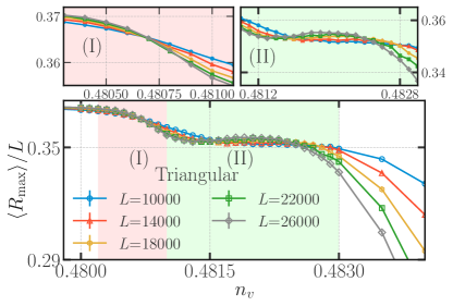
b)

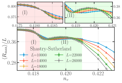
Figure 12: (a,b) $\langle R_{\rm max}\rangle/L$, the scaled radius of gyration (scaled with the system size $L$) of the largest Gallai-Edmonds cluster (either a ${\mathcal{R}}$-type region or a ${\mathcal{P}}$-type region) in ${\mathcal{G}}$ (the largest geometrically connected component of the diluted lattice) grows as the dilution $n_{v}$ is reduced. In the vicinity of the crossover visible in the probability $P_{\rm single}$ (see Fig. 14) of a Gallai-Edmonds cluster to wrap around the torus in exactly one direction, $\langle R_{\rm max}\rangle$ also shows non-monotonic crossover behavior. At the critical point identified earlier (see Fig. 8) via the threshold behavior of $P_{\rm cross}$, the probability for a cluster to wrap around the torus in two independent directions, $\langle R_{\rm max}\rangle/L$ also shows a well-defined crossing, with curves corresponding to different sizes crossing at the critical dilution $n_{v}^{\rm crit}\approx 0.4807$ [$n_{v}^{\rm crit}\approx 0.4182$] on the triangular [Shastry-Sutherland] lattice. The color-coded insets zoom in on the crossover region (in green) and on this critical region (in pink). See Sec. IV.2 for details.

Next, we ask some basic questions related to the geometry of ${\mathcal{R}}$-type and ${\mathcal{P}}$-type regions of the lattice, which we construct as indicated earlier using the e-type, u-type and o-type labels obtained from the Gallai-Edmonds decomposition. We begin with examining $m_{\rm tot}^{\mathcal{R}}$, the fraction of sites occupied by ${\mathcal{R}}$-type regions. From the upper panels of Fig. 3, we see that this quantity is nonzero in the thermodynamic limit and has only a very mild $n_{v}$ dependence; again the displayed data is in a narrow range of $n_{v}$, but we have checked this continues to be the case at lower values of $n_{v}$. The most striking feature of the data in Fig. 3 is clearly not its $n_{v}$ dependence. Rather, it is the noisy nature of the displayed data below some threshold value of $n_{v}$.

We emphasize that data at all $n_{v}$ displayed in Fig. 3 was obtained by averaging over the same number of samples at each $n_{v}$ (with a larger number of samples at smaller sizes and vice versa). So the reason for the noisy character of the data at lower values of $n_{v}$ is not poorer sampling of the disorder ensemble. Rather, it is a dramatic change in the distribution of $m_{\rm tot}^{\mathcal{R}}$. This is evident from the lower panels of Fig. 3. Below a threshold value of $n_{v}$, $m_{\rm tot}^{\mathcal{R}}$ has a bimodal distribution, with two sharply-defined and well-separated peaks. This separation between the peaks indicates a macroscopic difference in the morphology of the corresponding samples (since $m_{\rm tot}^{\mathcal{R}}$, as defined by us, is an intensive fraction or density), a difference that survives in the thermodynamic limit.

To understand this better, we now separate samples by asking which of the two peaks each sample belongs to. This is unambiguous because the peaks are well-separated even at the smallest size we study. Samples belonging to the peak with larger $m_{\rm tot}^{\mathcal{R}}$ are labeled ${\mathcal{R}}$-type, and those in the peak with smaller $m_{\rm tot}^{\mathcal{R}}$ are labeled ${\mathcal{P}}$-type. With this separation in place, we now examine the statistics of other observables within each of these two groups of samples.

When analyzed in this manner, the data paints a very clear picture: For instance, we see that samples with a high value of $m_{\rm tot}^{\mathcal{R}}$ always have a low value of $m_{\rm tot}^{\mathcal{P}}$ and vice-versa; this is shown both for the triangular lattice and the Shastry-Sutherland lattice in Fig. 4 for representative values of dilution in the bimodal regime. Thus, there is a two-peak structure in the histogram of $m_{\rm tot}^{\mathcal{P}}$ which is perfectly anti-correlated with the corresponding feature in the histogram of $m_{\rm tot}^{\mathcal{R}}$.

We find a similar dichotomy in the behavior of $n_{{\mathcal{R}}}$ and $n_{{\mathcal{P}}}$ in the two groups of samples on both lattices in this bimodal regime, with ${\mathcal{R}}$-type samples having a significantly higher value of $n_{{\mathcal{P}}}$ and a significantly lower value of $n_{{\mathcal{R}}}$ compared to ${\mathcal{P}}$-type samples. Thus, the distributions of $n_{{\mathcal{R}}}$ and $n_{{\mathcal{P}}}$ also have two well-separated peaks, with ${\mathcal{R}}$-type samples contributing solely to one peak and ${\mathcal{P}}$-type samples contributing only to the other peak. This is illustrated in Fig. 5 for the case of the triangular lattice at one representative value of the dilution in this bimodal regime.

At the risk of belaboring what is perhaps already obvious by now, we also study the histogram of $m_{\rm max}^{{\mathcal{R}}}$ and $m_{\rm max}^{{\mathcal{P}}}$ in both groups of samples. Again, we find perfectly correlated bimodal behavior. In ${\mathcal{R}}$-type samples the histogram of $m_{\rm max}^{{\mathcal{R}}}$ has a single peak at a fairly large $L$-independent value. The same is true of $m_{\rm max}^{{\mathcal{P}}}$ in ${\mathcal{P}}$-type samples. However, the histogram of $m_{\rm max}^{{\mathcal{R}}}$ in ${\mathcal{P}}$-type samples displays a peak at a very low value, which continuously shifts to even lower values with increasing $L$. The behavior of $m_{\rm max}^{{\mathcal{P}}}$ in ${\mathcal{R}}$-type samples is analogous. This is illustrated in Fig. 6 for the triangular lattice, again at the same representative value of $n_{v}$ in this bimodal regime.

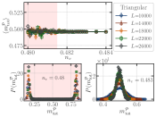
b)

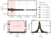
Figure 16: The sample-averaged total mass density of ${\mathcal{P}}$-type regions, ${m_{\rm tot}^{\mathcal{P}}}$, is nonzero and size-independent in the large $L$ limit. However, it develops large sample to sample fluctuations below a threshold value of $n_{v}$. (a) The figure on the left zooms in on this behavior in the vicinity of this threshold for the triangular lattice (b) The figure on the right zooms in on the corresponding threshold for the Shastry-Sutherland lattice. The bottom panels of (a) and (b) display histograms that represent our numerical estimate of the corresponding probability distribution $P(m^{{\mathcal{P}}}_{\rm tot})$ at representative values of $n_{v}$ above and below this threshold. From these histograms, it is clear that the large sample to sample fluctuations seen below the threshold are actually caused by a bimodality in this probability distribution, as evidenced by two widely separated narrow peaks. This bimodality should be contrasted with the single peak seen above the threshold. See Sec. IV.1 for details.

From this data analysis, we thus have a clear picture of a somewhat remarkable phenomenon: the morphology of ${\mathcal{R}}$-type and ${\mathcal{P}}$-type regions shows a complete lack of self-averaging even in the thermodynamic limit, when the dilution $n_{v}$ lies below a threshold. Additional numerical evidence that provides further details about the bimodal distributions of ${m_{\rm tot}^{\mathcal{P}}}$, ${n_{\mathcal{R}}}$, and ${n_{\mathcal{P}}}$ is shown in the Appendix in Fig. 16,  17 and  18.

Having established this unusual lack of self-averaging, we now proceed to rule out the most obvious possibility for its underlying cause. We have in mind here the parity of $m_{{\mathcal{G}}}$, i.e. whether the total number of sites in the largest geometric component ${\mathcal{G}}$ is odd or even. Fig. 7 shows the connected correlation function of the variables $\sigma$ and $\tau$. Here, the ${\mathcal{R}}$-type or ${\mathcal{P}}$-type character of a particular sample is encoded in the value of the variable $\sigma$, with $\sigma=1$ for ${\mathcal{R}}$-type samples and $\sigma=0$ for ${\mathcal{P}}$-type samples. Similarly, the parity of $m_{\mathcal{G}}$ is encoded in the value of the variable $\tau$, with $\tau=0$ for even parity and $\tau=1$ for odd parity. From the results displayed in Fig. 7, we see that our data for the connected correlation function $C(\sigma,\tau)$ is consistent with vanishingly small correlations (within our error bars). Hence, the parity of the largest geometric cluster ${\mathcal{G}}$ plays no role in the bimodality of various observables. Further, since $m_{\rm max}^{{\mathcal{R}}}$ ($m_{\rm max}^{{\mathcal{P}}}$) appears to saturate to a nonzero value in the thermodynamic limit of ${\mathcal{R}}$-type (${\mathcal{P}}$-type) samples, the threshold at which this bimodality sets in appears to reflect some kind of unusual percolation transition.

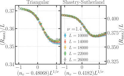
Figure 13: Data for the dimensionless ratio $R_{\rm max}(n_{v},L)/L$, where $R_{\rm max}(n_{v},L)$ is the sample-averaged radius of gyration of the largest GE cluster in ${\mathcal{G}}$ for two dimensional $L\times L$ samples, for various $L$ and $n_{v}$ collapses onto a single scaling curve when plotted against the scaling variable $(n_{v}-n_{v}^{\rm crit})L^{1/\nu}$. See Sec. IV.2 for details.

IV.2 Gallai-Edmonds percolation

To pin this down, we turn now to a study of the probability $P_{\rm cross}$, the probability that there is a cluster (either ${\mathcal{R}}$-type region or ${\mathcal{P}}$-type region) that wraps in two independent directions around the torus. We find, as shown in Fig. 8 that there is a sharply-defined value $n_{v}^{\rm crit}$ of the dilution at which the curves corresponding to different sizes all cross each other. This is the expected behavior at a critical point, and we identify this crossing point with the location of the Gallai-Edmonds percolation transition.

Next, we ask if this sharply-defined critical value also corresponds to a corresponding signature of a percolation transition in the susceptibility $\chi$. We find that $\chi/L^{2}$ tends to a nonzero value in the large $L$ limit for $n_{v}$ well below $n_{v}^{\rm crit}$. This is clear from Fig. 10. Further, we find that curves of $\chi/L^{2-\eta}$ cross at a threshold value of dilution that is within errors the same as the previous estimate of $n_{v}^{\rm crit}$, where $\eta$ is the anomalous exponent which takes on the value $\eta\approx 0.09(2)$. This is shown in inset of Fig. 10.

We now ask if data for $P_{\rm cross}$ and $\chi$ in the vicinity of this threshold displays finite-size scaling behavior. To this end, we construct the scaling variable $(n_{v}-n_{v}^{\rm crit})L^{1/\nu}$ where $\nu$ is the correlation length exponent, and ask if all our data for the $n_{v}$ dependence of $P_{\rm cross}$ at various sizes $L$ in the vicinity of this threshold collapses onto a single scaling curve for some choice of $\nu$. We find that this is indeed the case, for $\nu\approx 1.45(5)$ [$\nu\approx 1.50(5)$] on triangular [Shastry-Sutherland] lattice. This is shown in Fig. 9. Next we check if the data at various $L$ for $\chi/L^{2-\eta}$ also crosses at the same critical dilution for some value of $\eta$. We find that this is indeed the case, with $\eta\approx 0.09(2)$ as displayed in Fig. 10. In addition, we find that this quantity collapses onto a single scaling curve in the vicinity of $n_{v}^{\rm crit}$ when plotted against the scaling variable $(n_{v}-n_{v}^{\rm crit})L^{1/\nu}$, with $\nu\approx 1.50(7)$ for both the lattices. In Fig. 11 we see that this is indeed the case.

Thus, we have a fairly consistent picture of a critical point at $n_{v}^{\rm crit}\approx 0.48068(2)$ [ $n_{v}^{\rm crit}\approx 0.41820(5)$] on triangular [Shastry-Sutherland] lattice that separates a high-dilution phase in which all ${\mathcal{R}}$-type and ${\mathcal{P}}$-type regions are small from a low-dilution phase in which each sample has one infinite cluster, which can either be an ${\mathcal{R}}$-type cluster or an infinite ${\mathcal{P}}$-type cluster, on triangular [Shastry-Sutherland] lattice. This critical point is characterized by exponents $\nu\approx 1.45(9)$ and $\eta\approx 0.09(2)$ on both lattices. Curiously, this estimate of $\nu$ is quite close to (but not consistent with) the exact value of the correlation length exponent $\nu=4/3$ at the ordinary geometric percolation transition in two dimensions  [50, 51, 52, 53]. In contrast, our value of $\eta$ is very different from the value of the corresponding anomalous exponent $\eta=5/24$ at the geometric percolation transition in two dimensions.

a)

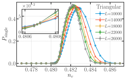
b)

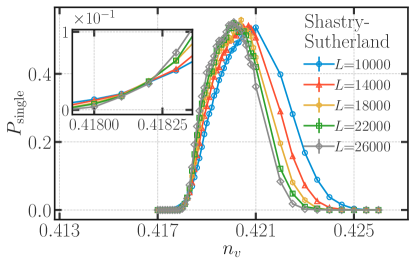
Figure 14: $P_{\rm single}$ is the probability that there exists a Gallai-Edmonds cluster (either a ${\mathcal{R}}$-type region or a ${\mathcal{P}}$-type region) in ${\mathcal{G}}$ (the largest geometrically connected component of the diluted lattice) which wraps around the torus in exactly one direction. Our data reveals threshold behavior in $P_{\rm single}$, with the threshod getting sharper with increasing system size. $P_{\rm single}$ vanishes with increasing size on the low-dilution side of this threshold. On the high-dilution side, it displays more complex non-monotonic behavior: As one approaches the threshold from above, $P_{\rm wrap}$ first develops a peak at an approximately size-independent value less than $1$. The position of this peak is $L$-dependent, and shifts to lower values of dilution with increasing size. By comparing this behavior to the behavior seen earlier in the probability $P_{\rm cross}$ for a cluster to wrap simultaneously in two independent directions (see Fig. 8), we conclude that this crossover behavior is associated with the wrapping characteristics of large clusters when they first form: Below this crossover, large clusters are more likely to wrap around two independent directions of the torus, while above this crossover, clusters are too small to wrap in even one direction. The actual critical point that corresponds to the threshold behavior seen in $P_{\rm cross}$ (see Fig. 8) is at lower values of $n_{v}$, and occurs in a regime in which $P_{\rm single}$ decreases with $n_{v}$. The inset zooms in on the vicinity of this critical point, and shows that curves corresponding to various sizes $L$ all cross at a critical dilution $n_{v}^{\rm crit}\approx 0.4807$ [$n_{v}^{\rm crit}\approx 0.4182$] on the triangular [Shastry-Sutherland] lattice. See Sec. IV.2 for details.

Although this scaling analysis appears to be fairly conclusive, we note that the scaling collapse appears to deteriorate rather rapidly on the high-dilution side of the transition. To dig a little deeper into the underlying reason, we now study the $n_{v}$ dependence of $\langle R_{\rm max}\rangle$, the ensemble average of the radius of gyration of the largest Gallai-Edmonds cluster (either an ${\mathcal{R}}$-type region or a ${\mathcal{P}}$-type region). As $n_{v}$ is decreased towards $n_{v}^{\rm crit}$, we find that $\langle R_{\rm max}\rangle$ has interesting non-monotonic $n_{v}$ dependence at values of $n_{v}$ outside the critical scaling window of the previously identified critical point at $n_{v}^{\rm crit}$. In this range of $n_{v}$, $\langle R_{\rm max}\rangle/L$ for each $L$ has a local maximum, with the value of $n_{v}$ corresponding to this local maximum shifting to lower dilution with increasing size. This is evident from the data displayed in Fig. 12. It is this unusual non-monotonic dependence that appears to limit the range of validity of the finite-size scaling form for $n_{v}$ above $n_{v}^{\rm crit}$.

Since $\chi/L^{2}$ decreases with increasing $L$ in this range of $n_{v}$, it is clear that this region does not exhibit percolation in the conventional sense (i.e. does not have an infinite Gallai-Edmonds cluster in the thermodynamic limit). Nevertheless, the fact that the peak height at the local maximum of $\langle R_{\rm max}\rangle/L$ in Fig. 12 appears to be close to saturating at the largest value of $L$ accessed in our study suggests this behavior is associated with some other large-scale property of the Gallai-Edmonds clusters in this regime.

To explore this further, we now examine the behavior of $P_{\rm single}$, the probability that the sample has no Gallai-Edmonds cluster that wraps around the torus in two independent directions, but has a Gallai-Edmonds cluster that wraps around the torus in exactly one direction. We find that $P_{\rm single}$ displays a well-defined maximum in the range of $n_{v}$ that corresponds to the non-monotonic behavior and local maximum of $\langle R_{\rm max}\rangle/L$. This maximum shifts to lower and lower values of $n_{v}$ as $L$ is increased. The corresponding data is displayed in Fig. 14.

This, coupled with the fact that $\chi/L^{2}$ decreases with increasing $L$ in this regime, indicates that this regime is characterized by clusters that are large in terms of their linear dimension (as characterized by the radius of gyration), which are able to wrap around the torus in one direction, but do not have a mass that scales with $L^{2}$. The picture is thus in terms of ribbon-like clusters that develop as a precursor to the actual percolation transition at a lower value of dilution $n_{v}^{\rm crit}$. This appears more of a crossover phenomenon that precedes (on the high-dilution side) the actual percolation transition of Gallai-Edmonds clusters. Nevertheless, we caution that the range of sizes available to us does not make it possible to completely rule out the possibility that this is a distinct thermodynamic phase that flanks the low-diluted percolated phase.

Independent of this, we do find that curves for $P_{\rm single}$ corresponding to different values of $L$ also cross at the critical dilution $n_{v}^{\rm crit}$ corresponding to the actual percolation transition. This is seen more clearly in the inset of Fig. 14. In the vicinity of this crossing point, we also find that $P_{\rm single}$ displays finite-size scaling behavior, with a value of $\nu\approx 1.45(7)$ [$\nu\approx 1.50(7)$], on the triangular [Shastry-Sutherland] lattice, consistent with all other estimates of $\nu$ obtained from other observables. This is shown in Fig. 15.

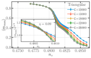
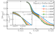
Figure 19: $m_{\rm max}$, the mass of the largest Gallai-Edmonds region inside ${\mathcal{G}}$ (the largest geometric cluster) in units of $m_{\mathcal{G}}$, the mass of ${\mathcal{G}}$, saturates to an $L$ independent value in the low-dilution phase. When scaled by $L^{-\eta/2}$, it shows a clear crossing at $n_{v}^{\rm crit}$. See Sec. IV.2 for details.

We have also examined the behavior of $\langle m_{\rm max}\rangle$, the ensemble average of the mass of the largest Gallai-Edmonds cluster (either ${\mathcal{R}}$-type or ${\mathcal{P}}$-type region) in a sample, as well as the behavior of the correlation length $\xi$ defined earlier. We find that these two show a clear signature of the percolation transition at $n_{v}^{\rm crit}\approx 0.48068(2)$ [$n_{v}^{\rm crit}\approx 0.41820(5)$] on triangular [Shastry-Sutherland] lattice and display finite-size scaling behavior with exponents $\nu=1.50(5)$ and $\eta=0.09(2)$ consistent within errors with the estimates for these exponents obtained from the observables studied above on both the lattices. The corresponding data and analysis is relegated to Figs. 19,  20,  22 and  22 in the Appendix.

V Outlook

The unusual percolation transition identified here leads to several natural and interesting questions, and it is perhaps useful to close with a brief discussion of some of them although we are not in a position to answer them here. These questions are of two types, one having to do with the actual wavefunctions of the topologically protected collective Majorana modes of disordered Majorana networks, and the other having to do with aspects of the Gallai-Edmonds decomposition of the corresponding disordered graph.

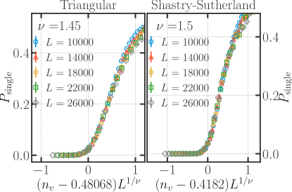
Figure 15: Data for $P_{\rm single}(n_{v},L)$, the probability that there exists a GE cluster $\in{\mathcal{G}}$ that wraps around the torus in one independent direction only for two dimensional $L\times L$ samples, for various $L$ and $n_{v}$ collapses onto a single scaling curve when plotted against the scaling variable $(n_{v}-n_{v}^{\rm crit})L^{1/\nu}$.Sec. IV.2 for details.

The most basic question regarding the mode wavefunctions is of course the question of their localization properties within a single ${\mathcal{R}}$-type region. Since each ${\mathcal{R}}$-type region ${\mathcal{R}}_{i}$ hosts ${\mathcal{I}}_{i}$ linearly independent such modes, the basis independent way of asking this question is to study the localization length of the imaginary part of the Green function. Is the correlation length of this Green function small compared to the typical size of ${\mathcal{R}}$-type regions in a ${\mathcal{R}}$-type sample in the low-dilution phase? If not, does the bimodality identified here lead to signatures in some physical observable that is sensitive to this correlation length? The answer is not obvious at all, since we have already seen that this bimodality or lack of self-averaging in the low-dilution phase has no discernible effect on the overall thermodynamic density $w$ of these modes (this is evident from the fact that the histogram of $w$ has a single well-defined peak even when there are two pronounced and macroscopically separated peaks in the histogram of ${m_{\rm max}^{\mathcal{R}}}$ for instance).

Another question that arises immediately is the relation between the unusual low-dilution phase identified here on the triangular lattice, and the large-scale structure of the Dulmage-Mendelsohn decomposition of the site-diluted square lattice in the corresponding dilution range. In the square lattice case, ${\mathcal{R}}_{A}$ and ${\mathcal{R}}_{B}$ type regions that host the monomers of maximum matchings and topologically protected zero modes of bipartite hopping problems grow in spatial extent as $n_{v}$ is reduced, but never percolate except in the limit $n_{v}\rightarrow 0$. This unusual incipient percolation phenomenon also occurs on the honeycomb lattice, and to that extent, appears to be universal. Importantly, ${\mathcal{P}}$-type regions appear to play no role in it at all, in the sense that their size remains small in this limit (of course, the entire pure sample is ${\mathcal{P}}$-type at $n_{v}=0$, so this statement is only true when the thermodynamic limit is taken keeping $n_{v}$ fixed at a small but nonzero value). The question then is: How does this regime, with incipient percolation of ${\mathcal{R}}_{A}$ and ${\mathcal{R}}_{B}$ regions and microscopically small ${\mathcal{P}}$-type regions go over to the unusual percolated phase found here on the triangular lattice when one randomly starts adding in some of the additional diagonal links needed to convert the square lattice into a triangular lattice? If the fraction of diagonal links added is denoted by $x$, then is there a critical value $x_{c}$ at which there is a percolation transition as a function of $x$? (with $n_{v}$ kept fixed in this low-dilution regime).

The third and equally immediate question has to do with the nature of the critical point. Based on the comparison of our results on the triangular and Shastry-Sutherland lattice, one may conclude that the large-scale behavior in the critical region is certainly universal. As mentioned earlier, our estimate of the corresponding correlation length exponent $\nu=1.45(7)$ of the Gallai-Edmonds percolation transition is, quite close to (but not consistent with) the exact value of the correlation length exponent $\nu=4/3$ at the ordinary geometric percolation transition in two dimensions  [50, 51, 52, 53]. In contrast, our value of $\eta$ is very different from the value of the corresponding anomalous exponent $\eta=5/24$ at the geometric percolation transition in two dimensions. This raises the questions: Is there a different continuum field theory description of the Gallai-Edmonds percolation transition? Does the Gallai-Edmonds critical point exhibit conformal invariance like the usual percolation transition in two dimensions?

These are some of the interesting questions that are brought to the fore by our study, and we hope to return to them in future work.

VI Acknowledgements

We gratefully acknowledge useful discussions with Mustansir Barma, Sounak Biswas, Deepak Dhar, Subhajit Goswami, and Piyush Srivastava. The work of RB was supported by a graduate fellowship of the DAE, India at the Tata Institute of Fundamental Research (TIFR). KD was supported at the TIFR by DAE, India and in part by a J.C. Bose Fellowship (JCB/2020/000047) of SERB, DST India, and by the Infosys-Chandrasekharan Random Geometry Center (TIFR). All computations were performed using departmental computational resources of the Department of Theoretical Physics, TIFR and additional resources supported by a J.C. Bose Fellowship grant (JCB/2020/000047). We gratefully acknoweldge the departmental system administrators K. Ghadiali and A. Salve, who have ensured the efficient utilization of these computational resources by their prompt actions and timely interventions.

*

Additional numerical evidence

a)

a)

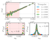
b)

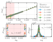
Figure 17: (a, b) The mean number density of ${{\mathcal{R}}}$-type regions, $n_{\mathcal{R}}$, of the Gallai-Edmonds decomposition is size-independent in large $L$ limit and decreases as we decrease dilution concentration $n_{v}$. However, it develops large sample to sample fluctuations below a threshold value of $n_{v}$. (a) The figure on the left zooms in on this behavior in the vicinity of this threshold for the triangular lattice (b) The figure on the right zooms in on the corresponding threshold for the Shastry-Sutherland lattice. The bottom panels of (a) and (b) display histograms that represent our numerical estimate of the corresponding probability distribution $P(n_{{\mathcal{R}}})$ at representative values of $n_{v}$ above and below this threshold. From these histograms, it is clear that the large sample to sample fluctuations seen below the threshold are actually caused by a bimodality in this probability distribution, as evidenced by two widely separated narrow peaks. This bimodality should be contrasted with the single peak seen above the threshold.See Sec. IV.1 for details.

a)

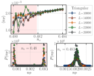
b)

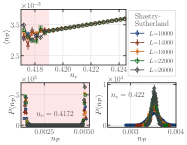
Figure 18: (a, b) The mean number density of ${{\mathcal{P}}}$-type regions, $n_{\mathcal{P}}$, of the Gallai-Edmonds decomposition is size-independent in large $L$ limit and decreases as we decrease dilution concentration $n_{v}$. However, it develops large sample to sample fluctuations below a threshold value of $n_{v}$. (a) The figure on the left zooms in on this behavior in the vicinity of this threshold for the triangular lattice (b) The figure on the right zooms in on the corresponding threshold for the Shastry-Sutherland lattice. The bottom panels of (a) and (b) display histograms that represent our numerical estimate of the corresponding probability distribution $P(n_{{\mathcal{P}}})$ at representative values of $n_{v}$ above and below this threshold. From these histograms, it is clear that the large sample to sample fluctuations seen below the threshold are actually caused by a bimodality in this probability distribution, as evidenced by two widely separated narrow peaks. This bimodality should be contrasted with the single peak seen above the threshold.See Sec. IV.1 for details.

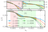
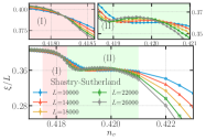
Figure 20: Data for the dimensionless ratio $\xi/L$, where $\xi$ is the correlation length associated with sample-averaged geometric correlation function $C(r-r^{\prime})$ in an $L\times L$ sample, shows a clear crossing at the critical dilution. In addition, it shows non-monotonic behavior very similar to that of $R_{\rm max}/L$ on the high-dilution side of the crossing. See Sec. IV.2 for details.

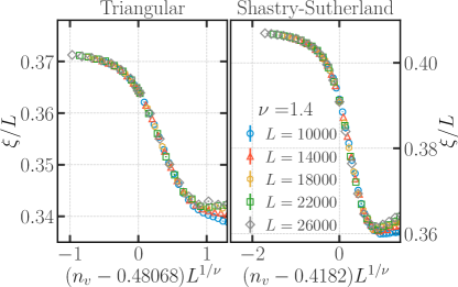
Figure 21: Data for the dimensionless ratio $\xi/L$, where $\xi$ is the correlation length associated with sample-averaged geometric correlation function $C(r-r^{\prime})$ in an $L\times L$ sample, collapses onto a single scaling curve when plotted against the scaling variable $(n_{v}-n_{v}^{\rm crit})L^{1/\nu}$ for a suitable choice of $n_{v}^{\rm crit}$ and $\nu$. See Sec. IV.2 for details.

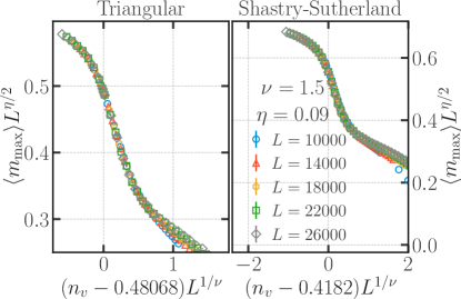
Figure 22: Figure shows $\langle m_{\rm max}\rangle$, the average mass of the largest Gallai-Edmonds region in the largest geometric cluster ${\mathcal{G}}$, scaled by $m_{\mathcal{G}}$, the mass of ${\mathcal{G}}$. We see that when our data for $m_{\rm max}$ is scaled by $L^{-eta/2}$ and plotted versus $(n_{v}-n_{v}^{\rm crit})L^{1/\nu}$, for appropriate choice of $\nu$ and $\eta$, it collapses onto a single scaling curve. See Sec. IV.2 for details.

References

- Read and Green [2000] N. Read and D. Green, Paired states of fermions in two dimensions with breaking of parity and time-reversal symmetries and the fractional quantum Hall effect, Phys. Rev. B 61, 10267 (2000).
- Ivanov [2001] D. A. Ivanov, Non-abelian statistics of half-quantum vortices in -wave superconductors, Phys. Rev. Lett. 86, 268 (2001).
- Kitaev [2001] A. Y. Kitaev, Unpaired Majorana fermions in quantum wires, Physics-Uspekhi 44, 131 (2001).
- Motrunich et al. [2001] O. Motrunich, K. Damle, and D. A. Huse, Griffiths effects and quantum critical points in dirty superconductors without spin-rotation invariance: One-dimensional examples, Phys. Rev. B 63, 224204 (2001).
- Sau et al. [2010] J. D. Sau, S. Tewari, R. M. Lutchyn, T. D. Stanescu, and S. Das Sarma, Non-Abelian quantum order in spin-orbit-coupled semiconductors: Search for topological Majorana particles in solid-state systems, Phys. Rev. B 82, 214509 (2010).
- Potter and Lee [2010] A. C. Potter and P. A. Lee, Multichannel generalization of Kitaev’s Majorana end states and a practical route to realize them in thin films, Phys. Rev. Lett. 105, 227003 (2010).
- McGinley et al. [2017] M. McGinley, J. Knolle, and A. Nunnenkamp, Robustness of Majorana edge modes and topological order: Exact results for the symmetric interacting Kitaev chain with disorder, Phys. Rev. B 96, 241113 (2017).
- Udagawa [2018] M. Udagawa, Vison-Majorana complex zero-energy resonance in the Kitaev spin liquid, Phys. Rev. B 98, 220404 (2018).
- Wen [2004] X.-G. Wen, Quantum Field Theory of Many-Body Systems (Oxford University Press, 2004).
- Laumann et al. [2012] C. R. Laumann, A. W. W. Ludwig, D. A. Huse, and S. Trebst, Disorder-induced Majorana metal in interacting non-Abelian anyon systems, Phys. Rev. B 85, 161301 (2012).
- Biswas [2013] R. R. Biswas, Majorana fermions in vortex lattices, Phys. Rev. Lett. 111, 136401 (2013).
- Affleck et al. [2017] I. Affleck, A. Rahmani, and D. Pikulin, Majorana-Hubbard model on the square lattice, Phys. Rev. B 96, 125121 (2017).
- Li and Franz [2018] C. Li and M. Franz, Majorana-Hubbard model on the honeycomb lattice, Phys. Rev. B 98, 115123 (2018).
- Kitaev [2006] A. Kitaev, Anyons in an exactly solved model and beyond, Annals of Physics 321, 2 (2006).
- Yao and Kivelson [2007] H. Yao and S. A. Kivelson, Exact chiral spin liquid with non-Abelian anyons, Phys. Rev. Lett. 99, 247203 (2007).
- Yao and Lee [2011] H. Yao and D.-H. Lee, Fermionic magnons, non-Abelian spinons, and the spin quantum Hall effect from an exactly solvable spin- Kitaev model with SU(2) symmetry, Phys. Rev. Lett. 107, 087205 (2011).
- Chua et al. [2011] V. Chua, H. Yao, and G. A. Fiete, Exact chiral spin liquid with stable spin Fermi surface on the kagome lattice, Phys. Rev. B 83, 180412 (2011).
- Lai and Motrunich [2011] H.-H. Lai and O. I. Motrunich, Power-law behavior of bond energy correlators in a Kitaev-type model with a stable parton Fermi surface, Phys. Rev. B 83, 155104 (2011).
- Fu [2019] J. Fu, Exact chiral-spin-liquid state in a Kitaev-type spin model, Phys. Rev. B 100, 195131 (2019).
- Sanyal et al. [2021] S. Sanyal, K. Damle, J. T. Chalker, and R. Moessner, Emergent moments and random singlet physics in a Majorana spin liquid, Phys. Rev. Lett. 127, 127201 (2021).
- Biswas et al. [2011] R. R. Biswas, L. Fu, C. R. Laumann, and S. Sachdev, SU(2)-invariant spin liquids on the triangular lattice with spinful Majorana excitations, Phys. Rev. B 83, 245131 (2011).
- Nayak et al. [2008] C. Nayak, S. H. Simon, A. Stern, M. Freedman, and S. Das Sarma, Non-Abelian anyons and topological quantum computation, Rev. Mod. Phys. 80, 1083 (2008).
- Alicea et al. [2011] J. Alicea, Y. Oreg, G. Refael, F. von Oppen, and M. P. A. Fisher, Non-Abelian statistics and topological quantum information processing in 1D wire networks, Nature Physics 7, 412 (2011).
- Stern and Lindner [2013] A. Stern and N. H. Lindner, Topological quantum computation—from basic concepts to first experiments, Science 339, 1179 (2013).
- Lovász and Plummer [1986] L. Lovász and M. D. Plummer, Matching Theory, Mathematics Studies 121 (North-Holland, Amsterdam, 1986).
- Damle [2022] K. Damle, Theory of collective topologically protected majorana fermion excitations of networks of localized majorana modes, Phys. Rev. B 105, 235118 (2022).
- Lovász [1979] L. Lovász, On determinants, matchings and random algorithms in Fundamentals of Computation Theory FCT’79, edited by L. Budach (Akademie-Verlag, Berlin, 1979) p. 565.
- Anderson [1975] W. N. Anderson, Jr., Maximum matching and the rank of a matrix, SIAM Journal on Applied Mathematics 28, 114 (1975).
- Gallai [1964] T. Gallai, Maximale Systeme unabhängiger Kanten, Magyar Tud. Akad. Mat. Kutató Int. Közl. 9, 401 (1964).
- Edmonds [1965] J. Edmonds, Paths, trees, and flowers, Canadian Journal of Mathematics 17, 449–467 (1965).
- Bhola et al. [2022] R. Bhola, S. Biswas, M. M. Islam, and K. Damle, Dulmage-Mendelsohn percolation: Geometry of maximally packed dimer models and topologically protected zero modes on site-diluted bipartite lattices, Phys. Rev. X 12, 021058 (2022).
- Broadbent and Hammersley [1957] S. R. Broadbent and J. M. Hammersley, Percolation processes: I. crystals and mazes, Mathematical Proceedings of the Cambridge Philosophical Society 53, 629–641 (1957).
- Stauffer and Aharony [1992] D. Stauffer and A. Aharony, Introduction to Percolation Theory (Taylor & Francis, London, 1992).
- Christensen and Moloney [2005] K. Christensen and N. R. Moloney, Complexity and Criticality (Imperial College Press, London., 2005).
- Duminil-Copin [2019] H. Duminil-Copin, Sharp threshold phenomena in statistical physics, Japanese Journal of Mathematics 15, 1 (2019).
- Bollobas and Riordan [2006] B. Bollobas and O. Riordan, Percolation (Cambridge University Press, Cambridge, 2006).
- Fortuin and Kasteleyn [1969] C. Fortuin and P. Kasteleyn, J. Phys. Soc. Jpn. Suppl. 26, 11 (1969).
- Fortuin and Kasteleyn [1972] C. Fortuin and P. Kasteleyn, On the random-cluster model: I. Introduction and relation to other models, Physica 57, 536 (1972).
- Chayes and Machta [1997] L. Chayes and J. Machta, Graphical representations and cluster algorithms I. Discrete spin systems, Physica A: Statistical Mechanics and its Applications 239, 542 (1997).
- Grimmett [2006] G. Grimmett, The Random-Cluster Model (Springer Berlin, Heidelberg, 2006).
- Grimmett [2018] G. Grimmett, Probability on Graphs: Random Processes on Graphs and Lattices (Cambridge University Press, Cambridge, 2018).
- Moret and Shapiro [1991] B. M. Moret and H. D. Shapiro, Algorithms from P to NP (vol. 1) design and efficiency (Benjamin-Cummings Publishing Co., Inc., Redwood City, CA,, 1991).
- Tarjan [1983] R. E. Tarjan, Data Structures and Network Algorithms (Society for Industrial and Applied Mathematics, Philadelphia, 1983).
- Kececioglu and Pecqueur [1998] J. D. Kececioglu and A. J. Pecqueur, Computing maximum-cardinality matchings in sparse general graphs, in Proceedings of the 2nd Workshop on Algorithm Engineering (1998).
- Bai and Breen [2008] L. Bai and D. Breen, Calculating center of mass in an unbounded 2D environment, Journal of Graphics Tools 13, 53 (2008).
- Newman and Ziff [2001] M. E. J. Newman and R. M. Ziff, Fast Monte Carlo algorithm for site or bond percolation, Phys. Rev. E 64, 016706 (2001).
- Pruessner and Moloney [2003] G. Pruessner and N. R. Moloney, Numerical results for crossing, spanning and wrapping in two-dimensional percolation, Journal of Physics A: Mathematical and General 36, 11213 (2003).
- Pruessner and Moloney [2004] G. Pruessner and N. R. Moloney, Winding clusters in percolation on the torus and the Möbius strip, Journal of Statistical Physics 115, 839 (2004).
- Sanyal et al. [2016] S. Sanyal, K. Damle, and O. I. Motrunich, Vacancy-induced low-energy states in undoped graphene, Phys. Rev. Lett. 117, 116806 (2016).
- Kesten [1987] H. Kesten, Percolation theory and first-passage percolation, The Annals of Probability 15, 1231 (1987).
- den Nijs [1979] M. P. M. den Nijs, A relation between the temperature exponents of the eight-vertex and q-state Potts model, Journal of Physics A: Mathematical and General 12, 1857 (1979).
- Nienhuis et al. [1980] B. Nienhuis, E. K. Riedel, and M. Schick, Magnetic exponents of the two-dimensional q-state Potts model, Journal of Physics A 13 (1980).
- Pearson [1980] R. B. Pearson, Conjecture for the extended Potts model magnetic eigenvalue, Phys. Rev. B 22, 2579 (1980).
*