Thermodynamic phases in first detected return times of quantum many-body systems

Abstract

We study the probability distribution of the first return time to the initial state of a quantum many-body system subject to stroboscopic projective measurements. We show that this distribution can be interpreted as a continuation of the canonical partition function of a spin chain with non-interacting domains at equilibrium, which is entirely characterised by the Loschmidt amplitude of the quantum many-body system. This allows us to show that this probability may decay either algebraically or exponentially asymptotically in time, depending on whether the spin model displays a ferromagnetic or a paramagnetic phase. We illustrate this idea on the example of the return time of $N$ adjacent fermions in a tight-binding model, revealing a rich phase behaviour, which can be tuned by scaling the probing time with $N$. Our analytical predictions are corroborated by exact numerical computations.

Introduction.— Measurements in quantum mechanics result in intrinsically stochastic outcomes and affect the quantum state [1, 2, 3, 4]. In particular, the first time at which a quantum state $\left|\Psi(t)\right\rangle$ is detected in a certain target state $\left|\Psi_{T}\right\rangle$ is a stochastic quantity of fundamental interest [5, 6], which depends on the measurement protocol. Recently, the probability of this first detection time under successive projective measurements has been studied extensively [7, 8, 9, 10, 11, 12, 13, 14, 15, 16, 17, 18, 19, 20, 21, 22, 23, 24, 25]. For a single quantum particle hopping on a line and subject to measurements at stroboscopic times $\tau,2\tau,3\tau,\dots$, the probability $F_{k}$ of first detection at time $k\tau$ at a certain position shows high sensitivity to the probing time $\tau$ [12, 13, 14, 15, 16]. In this case, $F_{k}$ features the quantum Zeno effect [26, 27] as $\tau\to 0$ and shows a rich behaviour depending on the position of the target state and whether it coincides with the initial state or not. In the former case, it further displays long-time universal behavior $F_{k}\sim k^{-3}$ [12, 13, 15] unlike its classical equivalent of the first-passage time [28]. All these works treat, however, single-particle systems, while the expected rich impact of quantum many-body dynamics on the universal properties of first-detection times has been, to our knowledge, not yet analyzed.

In this work, we address this problem by considering the case of the many-body first detected return time (FDRT), where the initial state coincides with the target state $\left|\Psi_{T}\right\rangle=\left|\Psi(0)\right\rangle$. We tackle this problem by developing a general and exact mapping of the quantum many-body FDRT probability $F_{k}$ onto the classical partition function of a one-dimensional spin model with non-interacting domains [29, 30, 31, 32, 33, 34, 35, 36]. Similar classical partition functions appear also in studied of the DNA melting transitions [29, 30, 31, 32] or in non-equilibrium currents [36]. This mapping allows us to classify the different asymptotic decays of $F_{k}$ as a function of $k$ in terms of the equilibrium phases of the classical partition function. Namely, we show that an algebraic decay corresponds to a ferromagnetic behavior, where large spin domains/long intervals of measurement-free evolution dominate $F_{k}$. On the contrary, an exponential decay of $F_{k}$ is found to correspond to the paramagnetic (disordered) phase of the classical spin model, where short domains/short measurement-free time intervals are relevant. We illustrate this approach by considering the case of $N$ adjacent fermions in a tight-binding model, which for $N=1$ reduces to previous studies [12, 13]. For finite $N$, we map this model onto the ferromagnetic phase of the truncated inverse square Ising model (TIDSI) [33, 37, 34, 35] and we exactly determine the asymptotic algebraic decay exponent $c_{N}$ of $F_{k}\sim k^{-2c_{N}}$. For $N=\infty$, instead, $F_{k}$ decays exponentially upon increasing $k$, which maps to paramagnetic behavior. Crucially, for finite $N$, we show that a crossover occurs from the aforementioned paramagnetic-exponential decay to a ferromagnetic-algebraic one. The corresponding crossover time increases upon increasing the number of $N$ of particles, an inherent feature of the quantum ballistic many-body nature of the dynamics. This crucially allows one to tune the onset of the algebraic decay of $F_{k}$ to more accessible short times and small particle numbers.

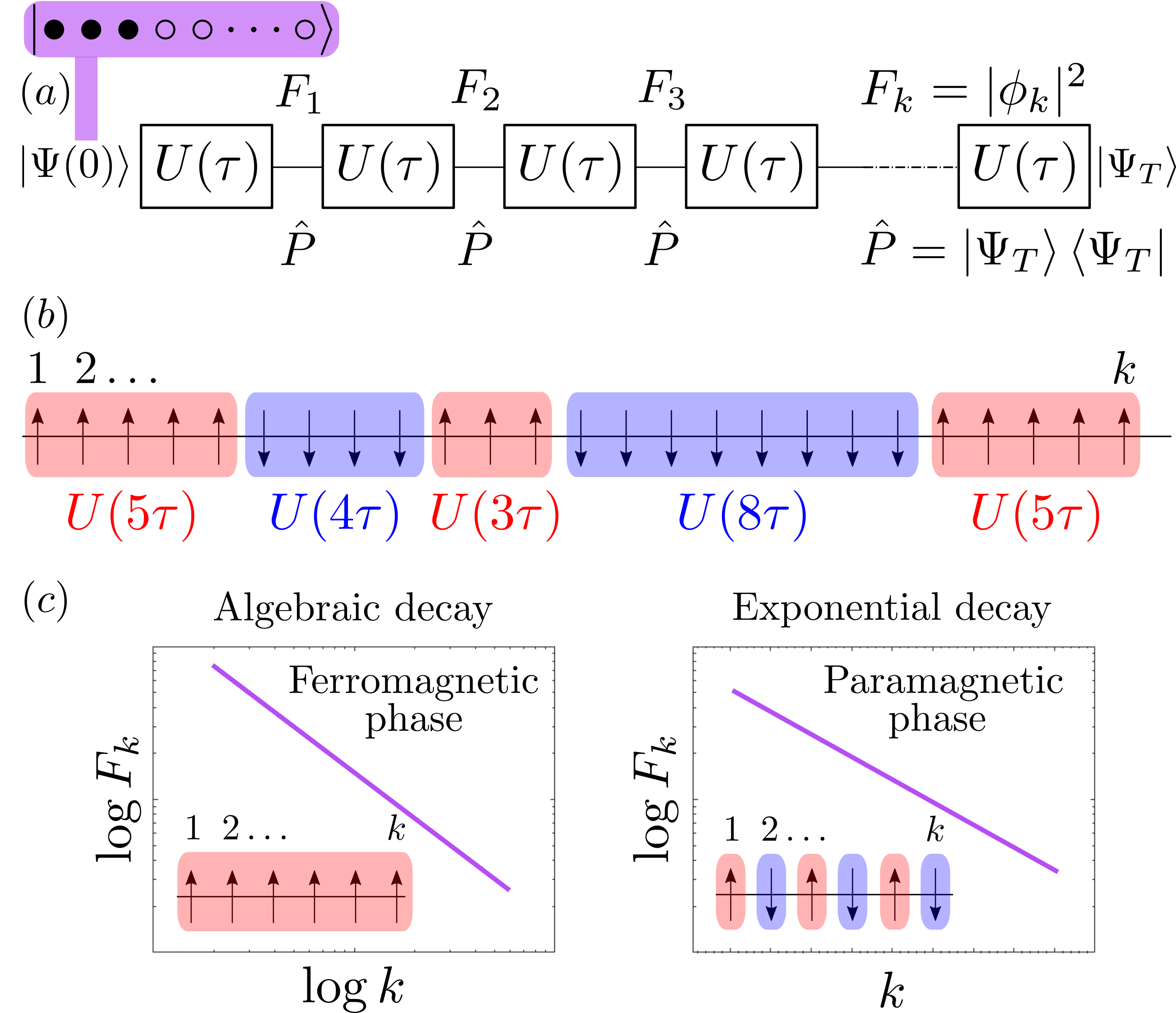
Figure 1: Quantum many-body first detection time. $(a)$ A wavefunction evolves with unitary dynamics $U(\tau)$ interspersed by projective measurements $\hat{P}$ occurring at stroboscopic times multiples of $\tau$. The target state $\left|\Psi\right\rangle_{T}=\left|\Psi(0)\right\rangle$ is first detected at the $k$th measurement with first detected return amplitude $\phi_{k}$ and probability $F_{k}=|\phi_{k}|^{2}$. The protocol terminates at the first successful detection in $\left|\Psi\right\rangle_{T}$. $(b)$ $\phi_{k}$ can be decomposed in terms of time intervals with no measurements and dynamics $U(n\tau)$ (in the figure $n=5,4,3,8$ and $5$, from left to right). Each interval can be mapped into a domain of aligned classical spins, with spins interacting via long-range interactions. Accordingly, $\phi_{k}$ is mapped onto a problem of statistical mechanics of domains at equilibrium in a volume $k$. $(c)$ When $F_{k}$ is determined by long measurement-free intervals $\sim U(k\tau)$, one has a ferromagnetic phase and $F_{k}$ decays algebraically upon increasing $k$. Conversely, when short intervals $\sim U(\tau)$ dominate, $F_{k}$ decays exponentially. This corresponds to the paramagnetic phase.

First detected return.— We study the FDRT probability of many-body systems described by an Hamiltonian $\mathcal{H}$, with associated unitary evolution $U(t)=e^{-i\mathcal{H}t}$. This problem can be tackled by extending the formalism developed in Refs. [12, 13] to the many-body realm, see Fig. 1$(a)$. Right before the first measurement at time $\tau$, the overlap of the wavefunction $\left|\Psi(\tau^{-})\right\rangle=U(\tau)\left|\Psi(0)\right\rangle$ with the target state $\left|\Psi(0)\right\rangle$ is given by the Loschmidt amplitude

$$\mathcal{L}(\tau)=\left\langle\Psi(0)\right|U(\tau)\left|\Psi(0)\right\rangle,$$ (1)

and therefore the detection is successful with probability $F_{1}=|\mathcal{L}(\tau)|^{2}$. In this case one has $\left|\Psi(\tau^{+})\right\rangle=\left|\Psi(0)\right\rangle$. If the detection is, instead, unsuccessful, the wavefunction is projected onto the space orthogonal to the target state and thus it reads $\left|\Psi(\tau^{+})\right\rangle=(\mathbb{1}-\hat{P})\left|\Psi(\tau^{-})\right\rangle/\sqrt{1-F_{1}}$, where $\hat{P}=\left|\Psi(0)\right\rangle\left\langle\Psi(0)\right|$, such that $\left\langle\Psi(\tau^{+})|\Psi(\tau^{+})\right\rangle=1$. Until the next measurement, the state evolves unitarily as $\left|\Psi(t)\right\rangle=U(t-\tau)\left|\Psi(\tau^{+})\right\rangle$ for $\tau<t<2\tau$, whence the procedure is reiterated until the first detection in the target state occurs.

The overlap between the wavefunction after $k-1$ unsuccessful detections and the target state immediately before the $k$th measurement defines the first detection amplitude

$$\phi_{k}=\left\langle\Psi(0)\right|U(\tau)\left[\left(\mathbb{1}-\hat{P}\right)U(\tau)\right]^{k-1}\left|\Psi(0)\right\rangle.$$ (2)

The FDRT probability $F_{k}$ is then given by $F_{k}=|\phi_{k}|^{2}$. The generating function $\hat{\phi}(z)=\sum_{k\geq 1}\phi_{k}z^{k}$ of $\phi_{k}$ is related to that $\hat{\mathcal{L}}(z)=\sum_{k\geq 1}\mathcal{L}_{k}z^{k}$ of $\mathcal{L}_{k}\equiv\mathcal{L}(k\tau)$ by [12, 13]

$$\hat{\phi}(z)=\frac{\hat{\mathcal{L}}(z)}{1+\hat{\mathcal{L}}(z)}.$$ (3)

The $\phi_{k}$’s are then determined as the integral

$$\phi_{k}=\oint\frac{{\rm d}{z}\,}{2\pi i}\frac{\hat{\phi}(z)}{z^{k+1}},$$ (4)

along a contour enclosing the origin $z=0$ and within the region of analyticity of $\hat{\phi}(z)$.

By expanding the $(k-1)$th power of $(\mathbb{1}-\hat{P})U(\tau)$ in Eq. (2), one finds that $\phi_{k}$ equals an alternating sum of measurement-free time intervals with evolution $U(\ell_{r}\tau)$ interspersed with $r$ projections $\hat{P}$, i.e., of terms of the form $\left\langle\Psi(0)\right|U(\ell_{1}\tau)\hat{P}U(\ell_{2}\tau)\ldots\hat{P}U(\ell_{r}\tau)\left|\Psi(0)\right\rangle$. One then has that

$$\phi_{k}=\sum_{r=1}^{k}(-1)^{r+1}\!\!\!\!\!\sum_{\ell_{1},\ell_{2},\ldots,\ell_{r}=1}^{\infty}\left(\prod_{j=1}^{r}\mathcal{L}_{\ell_{j}}\right)\delta_{\sum_{j=1}^{r}\ell_{j},k},$$ (5)

where $\delta_{n,m}=1$ for $n=m$ and 0 otherwise. Equation (5) is crucial to map the problem into the partition function of a classical lattice spin model with non-interacting domains, as sketched in Fig. 1$(b)$. A configuration of the spin model corresponds to a partition of the total volume $k$ into $r$ consecutive domains of lengths $\ell_{1},...,\ell_{r}$, with $\ell_{1}+...+\ell_{r}=k$ (see Fig. 1). To each domain, a length-dependent energy $E(\ell)$ is associated resulting from the possibly long-range interactions among the spins within the domain. The Boltzmann weight $w$ is associated, instead, to each domain wall. The canonical partition function of this model with fixed volume $k$ is given by

$$Z(k,w)=\sum_{r=1}^{k}w^{r+1}\!\!\!\!\!\sum_{\ell_{1},\ell_{2},\ldots,\ell_{r}=1}^{\infty}\left(\prod_{j=1}^{r}e^{-E(\ell_{j})}\right)\delta_{\sum_{j=1}^{r}\ell_{j},k}.$$ (6)

It is then apparent that Eq. (5) can be recovered from Eq. (6) by letting $w\to-1$ and by identifying the Loschmidt amplitude $\mathcal{L}_{\ell}=\mathcal{L}(\ell\tau)$ in time with the Boltzmann factor $e^{-E(\ell)}$ in space, with the stroboscopic period $\tau$ taking the role of the lattice spacing. Differently from the classical model, $E(\ell)=-\ln\mathcal{L}(\ell\tau)$ may now take complex values depending on the sign of $\mathcal{L}_{\ell}$, while $w=-1$ implies a purely imaginary energetic cost associated to a domain wall; these differences give rise to interferences when summed over, reflecting the quantum nature of $\phi_{k}$. The analogy extends to the fixed-pressure (grand canonical) ensemble. Summing over the length $k$, one obtains the partition function

$$\mathcal{Z}(z,w) =\sum_{k=1}^{\infty}z^{k}Z(k,w)=\frac{w^{2}\hat{\mathcal{L}}(z)}{1-w\hat{\mathcal{L}}(z)},$$ (7)

where $z$ is the exponential of the pressure conjugate to the length $k$, while $\hat{\mathcal{L}}(z)=\sum_{k\geq 1}e^{-E(k)}z^{k}$ is the grand canonical partition function of a single domain. Letting $w\to-1$ in Eq. (7), one recovers $\hat{\phi}(z)$ given in Eq. (3).

Emergence of phases.— In the thermodynamic limit $k\to\infty$, the spin model introduced in Eq. (6) may exhibit, depending on the form of $E(\ell)$ and on the value of $w$, either a ferromagnetic or a paramagnetic phase. This may happen even in one spatial dimension since $E(\ell)$ is determined by possibly long-range interactions among the spins within the domain. In the former case, the equilibrium ensemble is dominated by a globally ordered spin domain of length $\ell\sim\mathcal{O}(k)$, while in the latter the equilibrium is characterised by disordered spins with $\ell\sim\mathcal{O}(1)$. Identifying $\hat{\phi}(z)$ as $\mathcal{Z}(z,w\to-1)$ allows us to establish the possibility of observing two different behaviours of $\phi_{k}$ at large $k$, as shown in Fig. 1$(c)$. In fact, if the spin model is in the ferromagnetic phase, the dominant configuration is a global domain and thus $Z(k,-1)\sim e^{-E(k)}$; according to the mapping, this corresponds to the leading term of the first-detection amplitude being $\phi_{k}\sim\mathcal{L}(k\tau)$, see Eq. (5). This implies that the first successful detection is mainly due to uninterrupted unitary evolutions being projected onto the target state for the first time at $k\tau$. If the spin model is, instead, in the paramagnetic phase, and therefore it displays disordered domains, the partition function $Z(k,-1)\sim e^{-kE(1)}$ is dominated by short domains. In terms of the quantum evolution, this corresponds to $\phi_{k}\sim\mathcal{L}^{k}(\tau)$ being dominated by the product over many Loschmidt amplitudes of short duration, i.e., the typical wave function to be first detected at the $k$th attempt will have been projected back $\mathcal{O}(k)$ times to its initial state due to successive projective measurements.

The two cases mentioned above are understood through the analytic properties of $\hat{\phi}(z)=\mathcal{Z}(z,-1)$ as a function of $z$, which determines $\phi_{k}$ according to Eq. (4). The radius of convergence of $\hat{\phi}$ is controlled by its singularity at $z=z^{*}$, which is closest to the origin. By inspection of Eqs. (3) and (7), the singular point $z^{*}$ may arise from either $(i)$ a root in the denominator, i.e., $1+\hat{\mathcal{L}}(z^{*})=0$, leading to a simple pole or $(ii)$ a non-analyticity in $\hat{\mathcal{L}}(z^{*})$ leading to a branch point. If the singularity at $z^{*}$ is a simple pole, $\hat{\phi}(z)\sim(z-z^{*})^{-1}$, the integration in Eq.(4) renders $\phi_{k}\sim(z^{*})^{-k}$ and therefore an exponential dependence of $\phi_{k}$ on $k$. This exponential decay corresponds to the configuration with $k$ domains, i.e., to the paramagnetic phase. If the singularity $z^{*}$ is due to a branch point, instead, $\hat{\phi}(z)\sim|z-z^{*}|^{c-1}$ and via Tauberian scaling theorems one obtains an algebraic decay of $\phi_{k}\sim k^{-c}$ for large $k$ [38]. Algebraic growth of a canonical partition function in its volume is a consequence of a single domain in a long-range interacting spin model and thus we associate this behaviour with the ferromagnetic phase.

We illustrate this mapping by investigating the FDRT of $N$ free fermions with Hamiltonian $\mathcal{H}=\sum_{j=-\infty}^{\infty}\left(c_{j}^{\dagger}c_{j+1}+c_{j+1}^{\dagger}c_{j}\right)$, where $c_{j}$ and $c^{\dagger}_{j}$ are the fermionic annihilation and creation operators at site $j$, respectively. We consider an initial state $\left|\Psi(0)\right\rangle$ consisting of $N$ adjacent fermions on the lattice, corresponding to $\left|\Psi(0)\right\rangle=\otimes_{j=1}^{N}c_{j}^{\dagger}\left|0\right\rangle$, where $\left|0\right\rangle$ is the vacuum of the system (see the sketch in Fig. 1$(a)$). The case $N=\infty$ corresponds to a single domain wall at site $j=0$ separating the empty half-chain from the complementary filled one.

Ferromagnetic phase for finite $N$.— For finite $N$, $\mathcal{L}_{k}$ is the determinant of the matrix $\mathbb{J}_{N}(k\tau)=\left[i^{n-m}J_{m-n}(2k\tau)\right]_{m,n=1...N}$, where $J_{n}(x)$ is the $n$th Bessel function of the first kind [39]. In the limit of large time $k\tau$, the determinant $\mathcal{L}_{k}$ decays algebraically [39, 40]. According to the mapping to the classical spin model, the energy cost $E(\ell)=-\ln\mathcal{L}(\ell\tau)$ of a domain is, for $\tau\gtrsim 1$, logarithmic in $\ell$, i.e.,

$$E(\ell)=c_{N}\ln\ell+\Delta_{N}+(N\,{\rm mod}\,2)\ln\cos\left(2\ell\tau-N\pi/4\right),$$ (8)

where we introduced $c_{N}=(N^{2}+N\,{\rm mod}\,2)/4$ and $\Delta_{N}=c_{N}\ln\tau-\ln C_{N}$. Here $C_{N}=2^{\frac{N(N-2)}{4}}\pi^{-\frac{N}{2}}G^{2}\left(\frac{N+2}{2}\right)$ for even $N$, while $C_{N}=2^{\frac{(N-1)^{2}}{4}}\pi^{-\frac{N}{2}}G\left(\frac{N+1}{2}\right)G\left(\frac{N+3}{2}\right)$ for odd $N$, where $G(m)$ denotes Barnes’ $G$ function [41]. In general, $E(\ell)$ takes complex values.

Introducing the fugacity $y=e^{-\Delta_{N}}$, the grand canonical partition function of the spin model in Eq. (7) reads

$$\mathcal{Z}_{N}(z,w)=\frac{w^{2}y\Lambda_{N}(z)}{1-wy\Lambda_{N}(z)},$$ (9)

where $\Lambda_{N}(z)$ is determined in terms of the polylogarithm $\operatorname{Li}_{c_{N}}(z)=\sum_{k=1}^{\infty}z^{k}/k^{c_{N}}$ [40]. For $w=1$ and $N$ even, Eq. (9) equals the partition function of the truncated inverse distance squared Ising model (TIDSI) [33] which is parametrised by $y$ and $c_{N}$. This system undergoes a mixed-order phase transition from a paramagnetic to a ferromagnetic phase [33, 37, 34, 35]. In the quantum picture, however, we consider the partition function $\mathcal{Z}(z,w)$ at $w=-1$. For the spin model, this corresponds to studying the TIDSI model at the (classically forbidden) negative fugacity $-y$.

As detailed in Ref. [40], the leading singularity of $\mathcal{Z}_{N}$ in Eq. (9), is indeed due to generally separate branch points at $z^{*}_{\pm}=e^{\pm 2i\tau}$, which merge if $\tau$ is an integer multiple of $\pi/2$. The integral in Eq. (4) can then be carried out for all $N$, from which one obtains the leading large-$k$ behaviour of $\phi_{k}$ including its amplitude. For $N=1$, our analysis renders the results of Ref. [13]. For $N>1$, instead, it gives, up to some oscillating prefactor, $\phi_{k}\sim\mathcal{L}_{k}$ and thus the algebraic decay

$$\phi_{k}\sim k^{-c_{N}}\quad\mbox{and}\quad F_{k}\sim k^{-2c_{N}},$$ (10)

with logarithmic corrections for $N=2$ [40]. This algebraic behaviour is consistent with a ferromagnetic, globally ordered, phase in the spin model. Based on the energetic argument for the classical ferromagnetic phase, one can therefore understand the algebraic decay of $F_{k}$ in Eq. (10) as being the consequence of the corresponding slow decay (i.e., algebraic) of the Loschmidt amplitude, so that the first detected returns are predominantly due to free unitary evolutions $\phi_{k}\sim\mathcal{L}_{k}$. In Fig. 2$(a)$, we show the exact FDRT probabilities $F_{k}$ for $N=4$ and $6$, with fixed $\tau=2$, as obtained from the exactly known Loschmidt echo [40], which are compared with the expected leading algebraic behaviour (10), showing excellent agreement for large $k$.

Figure 2$(b)$ shows that the ratio $F_{k}/|\mathcal{L}_{k}|^{2}$ (symbols) is well captured by the branch cut asymptotics (solid line) for intermediate values of $\tau\gtrsim 1.8$ and large values of $k$. As $\tau\to 0$, the quantum Zeno regime is, instead, recovered [40].

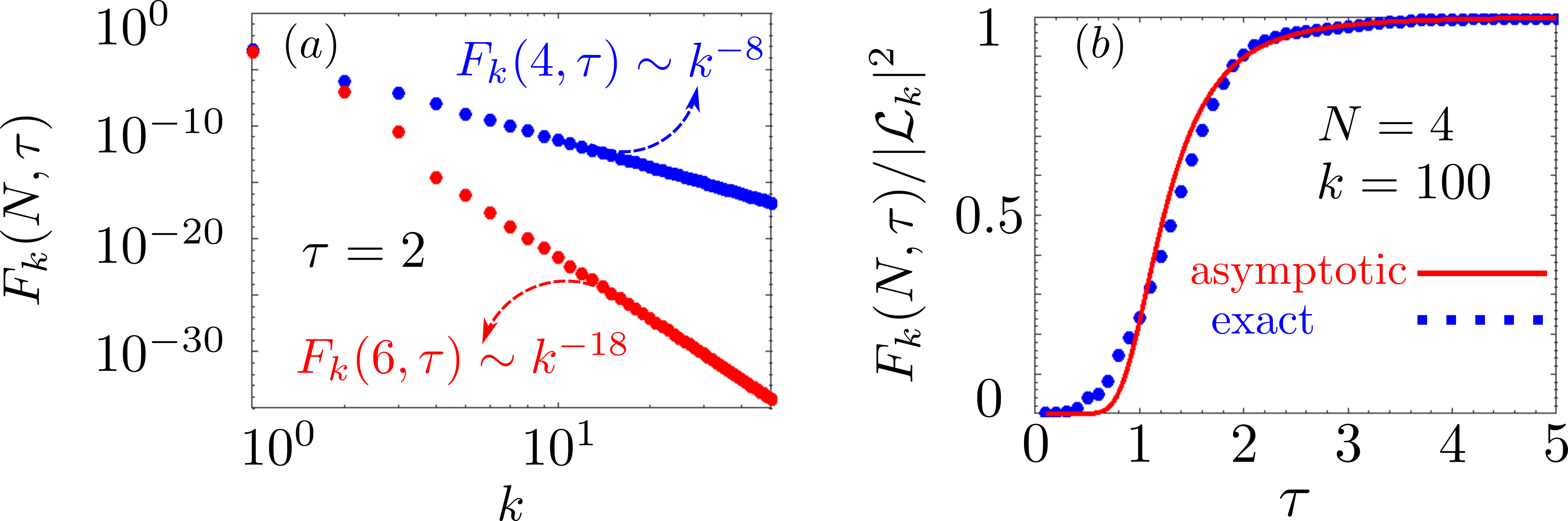
Figure 2: Ferromagnetic phase - algebraic decay. $(a)$ Log-log plot of the first detected return time probability $F_{k}$ as a function of $k$ for fixed stroboscopic time $\tau=2$, with $N=4$ and $6$. For sufficiently large $k\tau$, and according to the mapping on the paramagnetic phase of the spin model, $F_{k}\sim|\mathcal{L}_{k}|^{2}\sim k^{-2c_{N}}$ (with $c_{4}=4$ and $c_{6}=9$) decays algebraically upon increasing $k$. $(b)$ Ratio $F_{k}/|\mathcal{L}_{k}|^{2}$ (blue dots) as a function of $\tau$, for fixed $k=100$ and $N=4$ compared with the branch-cut asymptotic (red solid line).

Paramagnetic phase for $N=\infty$.— For a single domain wall, i.e., for $N=\infty$, the Loschmidt amplitude is exactly given by $\mathcal{L}(\tau)=e^{-\tau^{2}}$ [42, 39]. In the spin model this corresponds to a quadratic energetic cost of a domain, i.e., $E(\ell)=\tau^{2}\ell^{2}$. In order to evaluate $\mathcal{Z}_{N}(z,w)$ in Eq. (7), we introduce a partial theta function [43] $\Theta_{+}(z,q)=\sum_{k=1}^{\infty}z^{k}q^{k^{2}}$ in terms of which $\hat{\mathcal{L}}(z)=\Theta_{+}(z,e^{-\tau^{2}})$. Correspondingly, the grand canonical partition function is

$$\mathcal{Z}_{\infty}(z,w)=\frac{w^{2}\Theta_{+}(z,e^{-\tau^{2}})}{1-w\Theta_{+}(z,e^{-\tau^{2}})}.$$ (11)

As before, we need to understand the analytic properties of $\mathcal{Z}_{\infty}(z,-1)$ for complex $z$. For all $q\in(0,1)$, $\Theta_{+}(z,q)$ is an analytic function of $z$ [44], thus excluding branch cuts. In turn, for $w=-1$, $\mathcal{Z}_{\infty}$ has a countable set of poles at the complex roots $z_{n}$ of $1+\Theta_{+}(z_{n},q)=0$ [45]. For $q^{-2}\geq q_{\infty}=3.23\ldots$, these roots are simple, real and negative [46, 47], and they are approximately given, for large $n$, by $z_{n}=-q^{1-2n}$ [48]. This implies that for $\tau\geq\tau_{c}=\sqrt{(\ln q_{\infty})/2}=0.77\ldots$ the contour integral in Eq. (4) is given by the sum over all simple residues which is dominated, for large $k$, by the the root $z^{*}=z_{1}$ closest to the origin. One then finds $\phi_{k}\sim(z^{*})^{-k}$ for $\tau>\tau_{c}$ with a $k$-independent prefactor. This exponential decay is shown in Fig. 3$(a)$ for $\tau=0.8>\tau_{c}$. This behaviour corresponds to the paramagnetic phase in the spin model and can therefore be explained phenomenologically with the stronger quadratic growth of $E(\ell)$ upon increasing $\ell$, compared to the logarithmic growth for finite $N$ discussed previously. For $\tau<\tau_{c}$, the poles of $\mathcal{Z}_{\infty}$ are complex conjugate and therefore the dominating contribution stems from the closest conjugate pair $(z_{1},z_{1}^{*})$ of roots, leading to $\phi_{k}\propto C|z_{1}|^{-k-1}\cos\left((k+1)\arg(z_{1})\right)$. This is illustrated in Fig. 3$(a)$ where the exact values of $F_{k}$ (upper blue dots) display oscillations as functions of $k$ for $\tau=0.1<\tau_{c}$.

Asymptotically, for large $\tau$, the leading root of $1+\Theta_{+}(z,e^{-\tau^{2}})$ is given by $z^{*}\approx-e^{\tau^{2}}=-\mathcal{L}(\tau)$ such that $F_{k}\sim|\mathcal{L}(\tau)|^{2k}$, with the proportionality factor approaching 1 as $\tau\gtrsim 1$. The estimate of $F_{k}/|\mathcal{L}_{1}|^{2k}$ for $\tau>\tau_{c}$ can be systematically improved by applying Faà di Bruno’s theorem [49] to $\mathcal{Z}_{\infty}$, leading to an expansion in the maximal domain length $\ell_{\rm M}$ considered [40].

Figure 3: Paramagnetic phase - exponential decay. $(a)$ Log-linear plot of the first detected return time probability $F_{k}(\tau)\equiv F_{k}(N=\infty,\tau)$ of the semi-infinite occupied line as a function of $k$ for stroboscopic times $\tau=0.1$ (top-blue dotted) and $0.8$ (bottom-red dashed). $F_{k}$ decays exponentially upon increasing $k$, according to the mapping to the paramagnetic phase of the spin model. This exponential decay holds for all values of $\tau$. For $\tau<\tau_{c}=0.77\ldots$, $F_{k}$ features additional oscillations (blue symbols). $(b)$ Log-linear plot of the ratio $F_{k}(\tau)/|\mathcal{L}_{1}|^{2k}$ as a function of $\tau$ for fixed values of $k=10$ and 25. This ratio approaches $1$ upon increasing $\tau$ and, for $\tau>\tau_{c}$, it is well approximated by the systematic expansion (dashed-black lines) mentioned in the main text.

The estimates with $\ell_{\rm M}=3$ (dot-dashed lines, perturbative order $\mathcal{O}(e^{-12\tau^{2}})$) are compared in Fig. 3$(b)$ with the exact results of $F_{k}/|\mathcal{L}_{1}|^{2k}$ (solid lines), showing excellent agreement for $\tau>\tau_{c}$. At $\tau_{c}$, however, the asymptote breaks down and a sharp transition occurs into an oscillatory behaviour corresponding to the onset of imaginary roots in the partial theta function as shown also in Fig. 3$(a)$. In particular, Fig. 3$(b)$ shows that $F_{k}(\tau)$ vanish at $k-1$ special values of $\tau$ within the interval $(0,\tau_{c})$. These roots can be understood in terms of the entropically favourable formation of up to $r=1,2\dots k-1$ longer domains as $\tau$ is decreased. Due to the quantum nature of $Z_{\infty}(k,-1)$ (6), which requires $w\to-1$, the associated amplitudes interfere destructively leading to a vanishing $F_{k}=|Z_{\infty}(k,-1)|^{2}$.

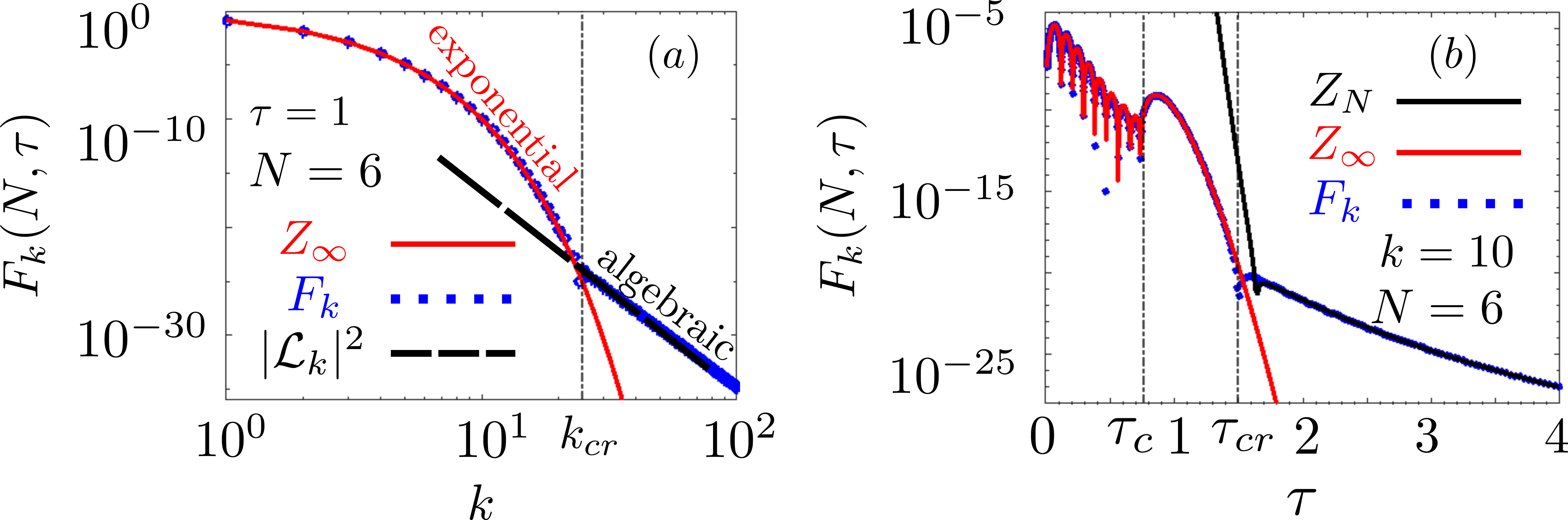
Figure 4: Phase crossover. $(a)$ Log-log plot of the first detection probability $F_{k}(N,\tau)$ as a function of $k$ for a fixed stroboscopic time $\tau=1$ and particle number $N=6$. For $\tau<\tau_{c}=0.77\ldots$, $F_{k}$ shows oscillations superimposed to the exponential decay as a function of $k$, as discussed in Fig. 3 for $N=\infty$. For $\tau>\tau_{c}$, instead, the decay is purely exponential, without oscillations. Upon increasing $k$, $F_{k}$ eventually shows a crossover from this exponential-paramagnetic to an algebraic-ferromagnetic decay. In this panel, the crossover occurs at $k=k_{cr}\approx 25$ for $N=6$, where $k_{cr}\sim N/\tau$. $(b)$ Log-linear plot of $F_{k}(N,\tau)$ as a function of $\tau$ for fixed $k=10$ and for $N=6$ fermions. For $\tau<\tau_{cr}$, with $\tau_{cr}\approx 1.5$, $F_{k}$ (blue dots) follows the behavior of the paramagnetic partition function $|Z_{\infty}(k,-1)|^{2}$ (red line), while for $\tau>\tau_{cr}$, $F_{k}(\tau)$ displays, up to some proportionality factor, the behavior of the ferromagnetic partition function $|Z_{N}(k,-1)|^{2}$ (black line). The crossover stroboscopic time scales as $\tau_{cr}\sim N/k$ upon increasing $N$.

Phase crossover and ferromagnetic transition.— We investigate here the onset of the ferromagnetic phase in $F_{k}$ upon increasing the measurement index $k$ beyond a crossover volume $k_{cr}$. For sufficiently small $k<k_{cr}$, $F_{k}$ is in perfect agreement with the paramagnetic behavior observed for $N=\infty$ fermions and predicted by $Z_{\infty}(k,-1)$ in Eq. (11). Upon increasing $k$ beyond $k_{cr}$, instead, $F_{k}$ sharply crosses over into the ferromagnetic behavior predicted by Eq. (9), where $F_{k}\sim|\mathcal{L}_{k}|^{2}$.

This crossover is illustrated in Fig. 4$(a)$ for $N=6$ and $\tau=1$. Note that, upon increasing $\tau$, the initial exponential decay might not be visible, as it happens in Fig. 2$(a)$ with $\tau=2$, where only the eventual algebraic behavior is seen. In a complementary way, Fig. 4$(b)$ shows that for a fixed value of $k=10$, larger values of $\tau>\tau_{cr}$ are needed in order for $F_{k}$ (blue-dotted curve) to be described by the ferromagnetic partition function in Eq. (9) (black-solid line).

For large $N$, this crossover from paramagnetic-like to ferromagnetic-like behaviour can be rationalized by studying the scaling limit of the Loschmidt amplitude $\mathcal{L}(\tau)$. Keeping $x=\tau/N$ finite, $\mathcal{L}(\tau)$ satisfies $\lim_{N\to\infty}N^{-2}\ln\mathcal{L}(Nx)=-f(x)$ where $f(x)\approx(\ln x)/4+3/8$ for $x\ll 1$ and $f(x)\approx x^{2}$ for $x\gg 1$ [39]. This fact implies that, upon rescaling the stroboscopic time $\tau$ with the number $N$ of fermions, the energy $E(k)=N^{2}f(k\tau/N)$ associated to a domain in the spin model may either grow logarithmically or quadratically as a function of $k$. Since this leads to either a ferro- or a paramagnetic behaviour in the thermodynamic limit, we conclude that the typical crossover chain volume $(k\tau)_{cr}$, above which $F_{k}$ decays algebraically, satisfies $(k\tau)_{cr}\sim N$. This linear scaling between space and time follows from the ballistic spreading of free fermions [50, 51, 52, 53, 42, 54, 55, 56, 57, 58, 59] and it is an inherent many-body feature, which enables to tune the onset of the ferromagnetic decay by scaling the probing time $\tau$ according to the number of particles.

Summary and outlook.— We proposed a mapping between the first detected return time (FDRT) of a many-body quantum system and the partition function of a classical system of magnetic domains in one spatial dimension. This mapping provides a physical explanation of the rich behavior of the probability of the FDRT which may display an algebraic (ferromagnetic) or an exponential (paramagnetic) decay at long times [see Fig. 1$(c)$]. The onset of the algebraic decay can be remarkably controlled by changing the duration of the stroboscopic time, making such a decay accessible already for relatively small times and particle number $N$, when the probability of the FDRT is still relatively large. At larger $N$, as expected, the probability of the FDRT becomes rapidly prohibitively small and its detection would require to devise more efficient detection protocols. For example, one may introduce resetting [23, 60, 61, 62, 63, 64, 65, 66, 25] in the protocol after a sequence of unsuccessful detections. Alternatively, one could consider the first detection time to attaining certain values of observables. In this respect, exploring the influence on the FDRT of possibly emerging collective behaviors such as at quantum critical points [67, 68, 69, 70, 71, 72] stands as an open problem for further investigation.

Acknowledgements.— BW would like to thank Giorgio Li, Adam Nahum, and Kay Wiese for insightful discussions. BW and AG acknowledge support from MIUR PRIN project “Coarse-grained description for non-equilibrium systems and transport phenomena (CO-NEST)” n. 201798CZL. BW further acknowledges funding from the Imperial College Borland Research Fellowship. GP acknowledges support from the Alexander von Humboldt foundation through a Humboldt research fellowship for postdoctoral researchers.

References

- Shankar [1994] R. Shankar, Principles of Quantum Mechanics, 2nd ed. (Springer, New York, NY, 1994).
- Jacobs [2014] K. Jacobs, Quantum measurement theory and its applications (Cambridge University Press, 2014).
- Breuer and Petruccione [2002] H.-P. Breuer and F. Petruccione, The theory of open quantum systems (Oxford University Press, 2002).
- Gardiner and Zoller [2010] C. W. Gardiner and P. Zoller, Quantum Noise: A Handbook of Markovian and Non-Markovian Quantum Stochastic Methods with Applications to Quantum Optics, 3rd ed., Springer Series in Synergetics (Springer, Berlin Heidelberg, 2010).
- Allcock [1969] G. R. Allcock, Ann. Phys. 53, 286 (1969).
- Kumar [1985] N. Kumar, Pramana 25, 363 (1985).
- Krovi and Brun [2006] H. Krovi and T. A. Brun, Phys. Rev. A 74, 042334 (2006).
- Grünbaum et al. [2013] F. A. Grünbaum, L. Velázquez, A. H. Werner, and R. F. Werner, Commun. Math. Phys. 320, 543 (2013).
- Dhar et al. [2015a] S. Dhar, S. Dasgupta, and A. Dhar, J. Phys. A: Math. Theor. 48, 115304 (2015a).
- Dhar et al. [2015b] S. Dhar, S. Dasgupta, A. Dhar, and D. Sen, Phys. Rev. A 91, 062115 (2015b).
- Sinkovicz et al. [2015] P. Sinkovicz, Z. Kurucz, T. Kiss, and J. K. Asbóth, Phys. Rev. A 91, 042108 (2015).
- Friedman et al. [2016] H. Friedman, D. A. Kessler, and E. Barkai, J. Phys. A: Math. Theor. 50, 04LT01 (2016).
- Friedman et al. [2017] H. Friedman, D. A. Kessler, and E. Barkai, Phys. Rev. E 95, 032141 (2017).
- Thiel et al. [2018a] F. Thiel, D. A. Kessler, and E. Barkai, Phys. Rev. A 97, 062105 (2018a).
- Thiel et al. [2018b] F. Thiel, E. Barkai, and D. A. Kessler, Phys. Rev. Lett. 120, 040502 (2018b).
- Thiel et al. [2019] F. Thiel, I. Mualem, D. A. Kessler, and E. Barkai, (2019), arxiv:1909.02114 [cond-mat, physics:quant-ph] .
- Liu et al. [2020] Q. Liu, R. Yin, K. Ziegler, and E. Barkai, Phys. Rev. Res. 2, 033113 (2020).
- Dittel et al. [2023] C. Dittel, N. Neubrand, F. Thiel, and A. Buchleitner, Phys. Rev. A 107, 052206 (2023).
- Thiel et al. [2020] F. Thiel, I. Mualem, D. Meidan, E. Barkai, and D. A. Kessler, Phys. Rev. Res. 2, 043107 (2020).
- Thiel and Kessler [2020] F. Thiel and D. A. Kessler, Phys. Rev. A 102, 012218 (2020).
- Dubey et al. [2021] V. Dubey, C. Bernardin, and A. Dhar, Phys. Rev. A 103, 032221 (2021).
- Das and Gupta [2022] D. Das and S. Gupta, J. Stat. Mech.: Theory Exp. 2022 (3), 033212.
- Yin and Barkai [2023a] R. Yin and E. Barkai, Phys. Rev. Lett. 130, 050802 (2023a).
- Yin and Barkai [2023b] R. Yin and E. Barkai, arXiv:2301.06100 (2023b).
- Kulkarni and Majumdar [2023] M. Kulkarni and S. N. Majumdar, arXiv:2305.15123 (2023).
- Misra and Sudarshan [1977] B. Misra and E. G. Sudarshan, J. Math. Phys. 18, 756 (1977).
- Chiu et al. [1977] C. B. Chiu, E. C. G. Sudarshan, and B. Misra, Phys. Rev. D 16, 520 (1977).
- Schrödinger [1915] E. Schrödinger, Phys. Z 16, 289 (1915).
- Poland and Scheraga [1966a] D. Poland and H. A. Scheraga, J. Chem. Phys. 45, 1456 (1966a).
- Poland and Scheraga [1966b] D. Poland and H. A. Scheraga, J Chem Phys 45, 1464 (1966b).
- Fisher [1984] M. E. Fisher, J. Stat. Phys. 34, 667 (1984).
- Richard and Guttmann [2004] C. Richard and A. J. Guttmann, J. Stat. Phys. 115, 925 (2004).
- Bar and Mukamel [2014a] A. Bar and D. Mukamel, Phys. Rev. Lett. 112, 015701 (2014a).
- Barma et al. [2019] M. Barma, S. N. Majumdar, and D. Mukamel, J. Phys. A: Math. Theor. 52, 254001 (2019).
- Mukamel [2023] D. Mukamel, Mixed Order Phase Transitions (2023), arxiv:2303.00470 [cond-mat] .
- Harris and Touchette [2017] R. J. Harris and H. Touchette, J. Phys. A: Math. Theor. 50, 10LT01 (2017).
- Bar and Mukamel [2014b] A. Bar and D. Mukamel, J. Stat. Mech. 2014, P11001 (2014b).
- Flajolet and Sedgewick [2009] P. Flajolet and R. Sedgewick, Analytic Combinatorics, 1st ed. (Cambridge University Press, 2009).
- Krapivsky et al. [2018] P. L. Krapivsky, J. M. Luck, and K. Mallick, J. Stat. Mech. 2018, 023104 (2018).
- Walter et al. [2023] B. Walter, G. Perfetto, and A. Gambassi, Supplemental material, in preparation (2023).
- Barnes [1901] E. W. Barnes, Philos. Trans. R. Soc. A 196, 265 (1901).
- Viti et al. [2016] J. Viti, J.-M. Stéphan, J. Dubail, and M. Haque, EPL 115, 40011 (2016).
- Andrews [1981] G. E. Andrews, Adv. Math. 41, 137 (1981).
- Kostov [2023] V. Kostov, Mat. Stud. 58, 142 (2023).
- Hardy [1905] G. H. Hardy, Proc. London Math. Soc. s2-2, 332 (1905).
- Katkova et al. [2004] O. M. Katkova, T. Lobova, and A. M. Vishnyakova, Comput. Methods Funct. Theory 3, 425 (2004).
- Kostov and Shapiro [2013] V. P. Kostov and B. Shapiro, Duke Math. J. 162, 825 (2013).
- Hutchinson [1923] J. I. Hutchinson, Trans. Amer. Math. Soc. 25, 325 (1923).
- Comtet [1974] L. Comtet, Advanced Combinatorics (Springer Netherlands, Dordrecht, 1974).
- Antal et al. [1999] T. Antal, Z. Rácz, A. Rákos, and G. Schütz, Phys. Rev. E 59, 4912 (1999).
- Platini and Karevski [2005] T. Platini and D. Karevski, Eur. Phys. J. B 48, 225 (2005).
- Collura and Martelloni [2014] M. Collura and G. Martelloni, J. Stat. Mech.: Theory Exp. 2014 (8), P08006.
- Allegra et al. [2016] N. Allegra, J. Dubail, J.-M. Stéphan, and J. Viti, J. Stat. Mech.: Theory Exp. 2016 (5), 053108.
- Bertini and Fagotti [2016] B. Bertini and M. Fagotti, Phys. Rev. Lett. 117, 130402 (2016).
- Eisler et al. [2016] V. Eisler, F. Maislinger, and H. G. Evertz, SciPost Phys. 1, 014 (2016).
- Kormos [2017] M. Kormos, SciPost Phys. 3, 020 (2017).
- Perfetto and Gambassi [2017] G. Perfetto and A. Gambassi, Phys. Rev. E 96, 012138 (2017).
- Ljubotina et al. [2019] M. Ljubotina, S. Sotiriadis, and T. Prosen, SciPost Phys. 6, 4 (2019).
- Perfetto and Gambassi [2020] G. Perfetto and A. Gambassi, Phys. Rev. E 102, 042128 (2020).
- Mukherjee et al. [2018] B. Mukherjee, K. Sengupta, and S. N. Majumdar, Phys. Rev. B 98, 104309 (2018).
- Riera-Campeny et al. [2020] A. Riera-Campeny, J. Ollé, and A. Masó-Puigdellosas, arXiv:2011.04403 (2020).
- Perfetto et al. [2021] G. Perfetto, F. Carollo, M. Magoni, and I. Lesanovsky, Phys. Rev. B 104, L180302 (2021).
- Perfetto et al. [2022] G. Perfetto, F. Carollo, and I. Lesanovsky, SciPost Phys. 13, 079 (2022).
- Turkeshi et al. [2022] X. Turkeshi, M. Dalmonte, R. Fazio, and M. Schirò, Phys. Rev. B 105, L241114 (2022).
- Magoni et al. [2022] M. Magoni, F. Carollo, G. Perfetto, and I. Lesanovsky, Phys. Rev. A 106, 052210 (2022).
- Belan and Parfenyev [2020] S. Belan and V. Parfenyev, New J. Phys. 22, 073065 (2020).
- Lamacraft and Fendley [2008] A. Lamacraft and P. Fendley, Phys. Rev. Lett. 100, 165706 (2008).
- Groha et al. [2018] S. Groha, F. H. L. Essler, and P. Calabrese, SciPost Phys. 4, 43 (2018).
- Collura and Essler [2020] M. Collura and F. H. L. Essler, Phys. Rev. B 101, 041110 (2020).
- Collura [2019] M. Collura, SciPost Phys. 7, 72 (2019).
- Calabrese et al. [2020] P. Calabrese, M. Collura, G. Di Giulio, and S. Murciano, EPL 129, 60007 (2020).
- Balducci et al. [2023] F. Balducci, M. Beau, J. Yang, A. Gambassi, and A. del Campo, arXiv:2307.02524 (2023).