Effective Data-Driven Collective Variables for Free Energy Calculations from Metadynamics of Paths

ABSTRACT. A variety of enhanced sampling methods predict multidimensional free energy landscapes associated with biological and other molecular processes as a function of a few selected collective variables (CVs). The accuracy of these methods is crucially dependent on the ability of the chosen CVs to capture the relevant slow degrees of freedom of the system. For complex processes, finding such CVs is the real challenge. Machine learning (ML) CVs offer, in principle, a solution to handle this problem. However, these methods rely on the availability of high-quality datasets – ideally incorporating information about physical pathways and transition states – which are difficult to access, therefore greatly limiting their domain of application. Here, we demonstrate how these datasets can be generated by means of enhanced sampling simulations in trajectory space via the metadynamics of paths [1] algorithm. The approach is expected to provide a general and efficient way to generate efficient high quality d CVs for the fast prediction of free energy landscapes. We demonstrate our approach on two numerical examples, a two-dimensional model potential and the isomerization of alanine dipeptide, using deep targeted discriminant analysis as our ML-based CV of choice.

Enhanced sampling (ES) methods [2, 3] are a powerful tool to investigate rare events in molecular systems, such as conformational changes of large biomolecular complexes, drug binding to receptor targets or phase transitions in materials [4, 5, 6]. To obtain the free energy landscape describing these complex phenomena, a large class of ES methods work under the assumption that a few collective variables (CVs), functions $s(\mathbf{R})$ of the atomic coordinates, exist that are able to provide a concise description of the transformation of interest. An external potential $V(s)$ can then be defined, able to drive the rare transitions and allowing a reconstruction of the free energy profile. These methods include, among many others, umbrella sampling [7], hyperdynamics [8], well-tempered or OPES-based metadynamics [9, 10, 11], adaptive biasing force [12], or variationally enhanced sampling [13]. We note here, that in cases where sufficiently long unbiased trajectories are available, researchers have designed general and elegant methods to describe the thermodynamics of a system without making use of CVs [14, 15]. However, being able to access the Boltzmann distribution from unbiased MD simulations is the exception rather than the rule.

The success of CV-based ES algorithms relies on the highly nontrivial choice of the CVs, which must be able not only to discriminate between the different metastable states, but also, and most importantly, to describe the progress of the reaction . Recently, machine learning-based (ML) methods have been shown to be effective in delivering CVs that fulfill these two criteria [16, 17, 18, 19, 20, 21, 22, 23, 24, 25]. However, as in any machine learning approach, the results depend dramatically on the quality of the underlying data. This leads to a chicken-and-egg problem: for good results, one ideally needs data on the relevant metastable states and transitions between them, which, in turn, would require knowledge of a CV that allows their thorough sampling [26]. As a result, most data-driven CV approaches still struggle to adequately accelerate the important motions in complex systems. To improve their efficiency, it has been previously recognized that including data from the transition state plays an important role in promoting the adequate description of the transition dynamics [27].

To harvest this essential data from the transition path ensemble, we shift our attention from enhanced sampling methods in configuration space to approaches focused on the direct sampling of the transition pathways. Among many such methods based on the statistical mechanics of trajectories [28, 29, 30], we consider the recently developed metadynamics of paths (MoP) algorithm [1]. In contrast to the popular transition path sampling [31, 32], which has also been used for the identification of CVs [33, 34, 24, 25], MoP allows for the unconstrained exploration of multiple reactive paths connecting metastable states without the need for an initial path guess. This is achieved by performing metadynamics simulations in the space of all trajectories, making use of special collective variables defined in trajectory space (CV_t hereafter). As we will see below, a crucial property of MoP is its robustness in sampling the transition path ensemble with respect to a suboptimal choice of this CV_t, considerably mitigating the chicken-and-egg problem described above.

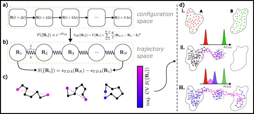
Figure 1: (a) A discrete stochastic trajectory consists of the time series $\{{\bf R}_{n}\}$ of configurations visited sequentially by the system. (b) To each discretized trajectory can be assigned a well-defined Boltzmann-like statistical weight $e^{-\beta V_{\rm eff}(\{{\bf R}_{n}\})}$. The effective potential is isomorphic to the potential energy of an elastic polymer. (c) One can generate all possible discretized trajectories of a physical system by evolving the dynamics of a fictitious polymer subject to the force $\mathcal{F}_{n}=-\nabla_{{\bf R}_{n}}V_{\rm eff}$. Metadynamics can be used to accelerate the sampling of reactive pathways by choosing an appropriate collective variable defined in trajectory space. Here, we adopt as CV_t the generalized polymer end-to-end distance $S$ of equation 3, defined as the difference between the Deep-TDA CV_c evaluated in the final and in the starting configuration of the polymer. (d) Iterative procedure for DeepTDA CV_c training. (i) Unbiased training data sets are generated in the initial (A) and final (B) states. A DeepTDA CV_c $s_{TDA}$ is trained to map the two datasets into well-separated Gaussian distributions. (ii) A MoP run is performed and the generated paths are classified as trapped (blue and black) and reactive (violet) paths, based on the value of $|S|$. New datasets are identified from newly discovered metastable states and from configurations occupying the transition state region. A multi-state DeepTDA CV_c is trained to map these configurations into well-separated distributions and a new end-to-end distance CV_t is built. (iii) The desired outcome of a MoP run using the refined end-to-end CV_t is depicted, showing sampling of trapped paths in all metastable states (in blue) as well as reactive pathways connecting different basins (in violet). This data can be used to design an optimal CV_c in configuration space to converge the free energy landscape in a standard metadynamics simulation.

We show that the data obtained from MoP can be used to train an efficient ML-based CV in configuration space (CV_c hereafter) to speed up standard metadynamics simulations. Here, among many different, powerful ML approaches, we use the deep targeted discriminant analysis (DeepTDA) supervised learning approach [35] previously developed to build CV_cs. Briefly, DeepTDA trains a classifier that discriminates configurations belonging to different metastable states by mapping them into well-separated, user-defined locations in latent space. This approach can be used to incorporate not only data from multiple metastable states, but also from reactive trajectories connecting them [35, 27]. The mapping is done such that the resulting one-dimensional CV_c describes the system’s progress from one basin to the other through the transition state region (see figure 1b, and SI for more details).

In practice, our proposed, iterative protocol (figure 1b) consists of the following steps:

1. Standard MD simulations lead to kinetically trapped conformations in the (assumed to be known) initial and final basins (figure 1b). A CV_c is obtained by training a DeepTDA model to discriminate these 2 states

2. Starting from such CV_c, a CV_t is built and MoP simulations are performed

3. The resulting trajectories are analyzed to identify newly discovered metastable states and reactive paths, and a new DeepTDA CV is trained including these data. If the latest MoP simulation found a path between initial and final states, the algorithm ends: it provides a complete map of the intermediate states and pathways of the molecular transform, which generally allows building efficient CV_c. Otherwise, step 2 is repeated with the new CV_c.

The method is designed to iteratively refine both CV_c and CV_t. More details on how the latter are constructed are provided below.

The paper is organized as follows: after an introduction to MoP and the definition of CV_t, we apply our iterative protocol (i) to a 2D model potential, used to test its applicability to multi-state systems, and (ii) to the isomerization of alanine dipeptide in vacuum, which, despite its simpler two-state nature, provides a non-trivial test case on a molecular system.

Metadynamics of paths

In standard MD simulations, a discrete trajectory – consisting of the time series $\{{\bf R}_{n}\}_{n=1,N}$ of configurations visited by the system – is generated in a sequential manner, due to the inherent seriality of the time evolution process (see Fig. 1a). MoP circumvents this problem – which rests at the base of the poor scaling of MD algorithms – and achieves parallelization in time by sampling directly from the phase space of all possible trajectories. The method applies to stochastic (Brownian) trajectories and exploits the isomorphism between the path probability distribution, $p[\mathcal{A}({\bf R}(t))]$, and the Boltzmann distribution of a fictitious elastic polymer (see Fig. 1b):

$$p[\mathcal{A}({\bf R}(t))]=\exp\left[-\beta V_{\rm eff}(\{{\bf R}_{n}\})\right]$$ (1)

$$V_{\rm eff}=U({\bf R}_{1})+\sum_{n=1}^{N-1}\frac{K}{2}\left({\bf R}_{n+1}-{\bf R}_{n}-{\bf L}_{n}\right)^{2}$$ (2)

In this equation, $\mathcal{A}$ is the Onsager-Machlup action [28], which is a functional of the (discretized) Brownian trajectory ${\bf R}(t)={\bf R}_{1}\rightarrow{\bf R}_{2}\rightarrow\dots\rightarrow{\bf R}_{N}$. $\beta=1/k_{B}T$, while $K=m\nu/2\Delta t$ and ${\bf L}_{n}=(m\Delta t/\nu){\bf F}_{n}$ are the effective spring constant and equilibrium length that depend on the physical parameters of the underlying Brownian dynamics: temperature $T$, mass $m$, damping coefficient $\nu$, time step $\Delta t$ (see SI for details). $U$ is the potential energy of the system and ${\bf F}_{n}=-\nabla U({\bf R}_{n})$ is the physical force acting on the $n$th configuration.

Finite temperature MD simulations of the polymer are performed by computing the fictitious forces ${\bf\mathcal{F}}_{n}=-\nabla_{{\bf R}_{n}}V_{\rm eff}$ acting on each configuration and are used to generate discretized trajectories distributed according to $p[\mathcal{A}({\bf R}(t))]$. Metadynamics, in turn, can be used to focus the sampling on the important reactive trajectories connecting metastable states. This requires defining CV_t in trajectory space.

Following Ref. [1], we define our CV_t as the generalized end-to-end distance

$$S(\{\mathbf{R}_{n}\})=s(\mathbf{R}_{N})-s(\mathbf{R}_{1}),$$ (3)

where, in this work, $s(\mathbf{R})$ is a DeepTDA CV_c. The rationale for this specific choice of $S$ is that it allows discriminating between elongated polymers (large values of $|S|$), which are likely to represent reactive trajectories, from kinetically trapped ones (with a low value of $|S|$), thus aiding in the discovery of new metastable states.

We note that reactive trajectories obtained from this method tend to spend more time in proximity to the transition states. This happens because the equilibrium spring constants are proportional to the physical force vector (${\bf L}_{n}\propto{\bf F}_{n}$) and, therefore, tend to zero close to the stationary points of the potential energy surface, including the unstable saddle points [30]. This feature increases the amount of data generated on transition states that can be used to train an efficient ML CV_c.

Two-Dimensional Model Potential

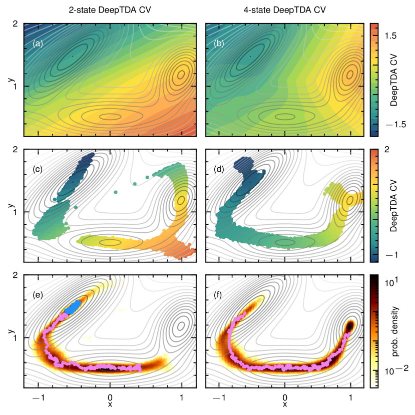
Figure 2: (a) Colored map showing the values of the initial 2-state DeepTDA CV_c. Initial, intermediate and final states are labeled as A, B and C, respectively. (b) Colored map of the 4-states DeepTDA CV_c. Scatter plots of $x,y$ coordinates are shown as obtained from an OPES simulation using (c) 2-state and (d) 4-state DeepTDA CV_c. Points colored according to the corresponding CV_c value. Configurations obtained from MoP simulations using (e) the initial 2-state and (f) the 4-state DeepTDA-based end-to-end distance CV_t are shown. The violet and blue paths show the most probable reactive and trapped trajectories, respectively, i.e., the ones attaining the lowest value of the Onsager-Machlup action (see SI for details). In all panels, the isolines of the model potential are shown in grey as a reference.

We first applied our iterative protocol to a particle moving in the two-dimensional model potential (adapted from Müller and Brown [36]) shown by the isolines of figure 2. The potential has three metastable states: an initial basin A and a final basin C which we assume to be known beforehand, and y an intermediate basin B. The relative positions of the three minima were designed to provide a scenario in which neither coordinate axis can resolve the transition states and drive the exploration of the whole free energy surface. Furthermore, in this case, a neural network CV simply trained to discriminate between the A and C is likely to fail, as demonstrated below.

We first performed unbiased simulations in the A and C basins and trained an initial 2-state DeepTDA CV_c. The value of the latter is shown by the colored map reported in figure 2a. Clearly, the intermediate metastable state B is not discriminated from the C basin since the CV attains the same value in the two basins. As a consequence, when used in an OPES simulation, we found that this CV_c is very inefficient in guiding transitions between A and C. Furthermore, during the simulation, the system is driven to sample unphysical trajectories that differ greatly from the minimum energy pathway (see figure 2c). As a result, we also observe that the free energy difference between basins A and C is not accurately estimated when compared to the analytical result obtained by numerical integration of the potential (see figure 3).

Nevertheless, we can employ this suboptimal CV to construct the end-to-end distance CV_t defined in equation 3 for use in a MoP simulation. The samples obtained from the simulation in trajectory space are reported in figure 2e. Notably, the sampled trajectories follow the underlying minimum energy pathways. This is due to the forces driving the polymer dynamics not being directly related to the potential energy surface but rather to the Onsager-Machlup action, which is lower for the more statistically relevant ones. By using the end-to-end distance CV_t, the metadynamics bias acts only on the polymer endpoints, while the intermediate replicas are free to relax minimizing the OM action. This illustrates the robustness of MoP in sampling physically relevant trajectories even when using suboptimal CV_t. Importantly, the analysis of the data allows blindly detecting the intermediate state from the presence of crumpled polymers confined entirely into this basin, which are characterized by small values of the end-to-end distance CV_t, $S\sim 0$.

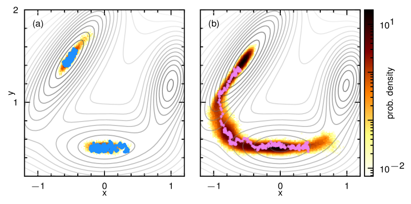
Figure S3: Trapped (a) and reactive (b) trajectories, isolated from a MoP simulation using the 2-state DeepTDA CV for the 2D model potential in trajectory space. Examples of trapped trajectories are shown in blue, a reactive trajectory in pink. The densities are calculated from 152 trapped and 1855 reactive trajectories, respectively. Isolines of the potential are indicated in grey.

Partial reactive trajectories connecting the A and B basins were also observed (see figure S3a). However, the simulation could not sample complete reactive paths connecting from A to C due to the suboptimal CV_c used in equation (3), which cannot distinguish correctly between B and C. We solve this problem by performing a second iteration of the algorithm in which the information gained from the MoP run is used to train a refined, 4-states DeepTDA CV, including data from the three metastable states plus the transition region between A and B (for all technical details we refer to the SI). The colored map of the new CV_c is shown in figure 2b. It is apparent that all relevant metastable and transition states are resolved.

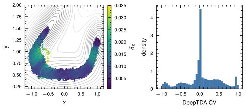
Figure S5: Trajectories sampled by MoP spend more time in the vicinity of transition states. (a) Moving average of the oriented displacement between adjacent beads in a trajectory (average adjacent displacement, or AAD). If $\{\mathbf{d}_{n}\}_{n=1}^{N}$ is a set of descriptors or CV_cs, at bead $n$ this measure is given by $\delta_{n}=\left|\frac{1}{2k}\sum_{m=-k}^{k}\mathbf{d}_{n-m+1}-\mathbf{d}_{n-m}\right|$, where $k$ is the kernel width of the moving average. Thereby, it directly shows regions of increased density along the polymer as regions of decreased AAD. Here it is evaluated along the reactive trajectories obtained from a MoP simulation using the 4-state DeepTDA CV_t, as described in the main text, with $k=15$. Note that AAD is decreased not only in the known metastable states A and C, but also in state B and on the transition states connecting them. (b) Histogram of the 4-state DeepTDA CV, evaluated on the reactive paths obtained in a MoP simulation. Note the peaks in the distribution around $s=-1,1$ corresponding to basins A and C, the sharp peak at $s=0$ corresponding to the intermediate basin B, and peaks around $s=-0.5,0.5$, corresponding to the transition states.

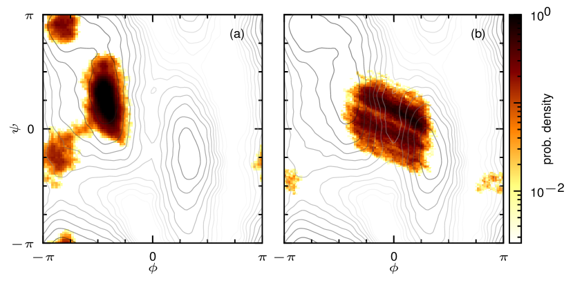
Figure S9: Trapped (a) and reactive (b) trajectories, isolated from a MoP simulation using the 3-state DeepTDA CV for alanine dipeptide in trajectory space. The normalized densities are calculated from 1405 trapped and 569 reactive trajectories, respectively. Isolines of the FES of alanine dipeptide calculated from a converged reference calculation using the $\phi,\psi$ dihedral angles are indicated in grey.

The new CV_c,t drives complete transitions from A to C both when used in MoP (figure 2f) as well as in standard OPES simulations (figure 2d). Figure 3 shows that the free energy difference between basins A and C, as estimated with the new CV_c, is in excellent agreement with the analytical result. We also checked that the corresponding end-to-end distance CV_t improves sampling in trajectory space. Figure 2f reports the result of a MoP simulation, showing the sampling of complete reactive trajectories connecting A and C along the minimum free energy path. The efficiency of this CV is further demonstrated by the fact that it was able to generate also the partial paths connecting basins A and B, and B and C (see figure S9). From the complete reactive paths, we can also observe that they indeed spend an increased amount of time in the vicinity of the transition state, as illustrated in figure S5.

The new dataset obtained from MoP allowed us to train a 5-states DeepTDA CV_c,t, also including data from the transition state between B and C. The resulting CVs, however, did not lead to significant improvements respect to the 4-states versions.

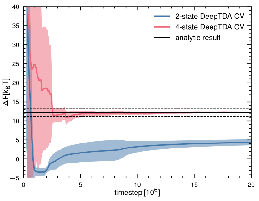
Figure 3: Free energy difference between the left and right basins of the model potential, as estimated from 5 independent OPES simulations biasing the 4-state DeepTDA CV, as a function of simulation time. The analytical result of $12.15\,k_{B}T$ was obtained by numerical integration over the MB potential [37] and is indicated in black, with dotted lines indicating a margin of $1\,k_{B}T$.

Alanine Dipeptide

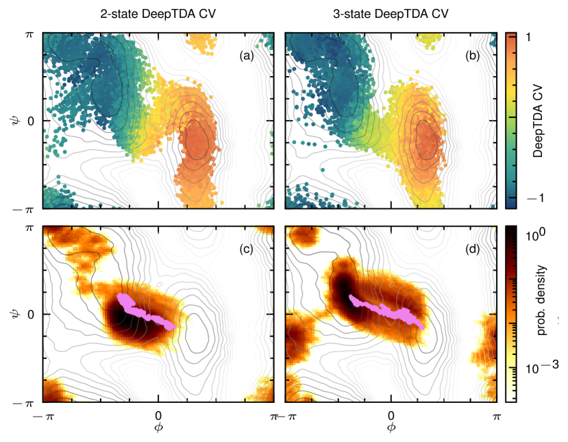
Figure 4: Biased simulations in configuration and trajectory space of alanine dipeptide. Scatter plots of $x,y$ coordinates in OPES simulation using (a) 2-state and (b) 3-state DeepTDA CV_c are shown, colored according to CV value. MoP simulations using (c) initial and (d) 3-state DeepTDA CV_t are shown, shown as normalized density of all configurations in logarithmic scale. The violet paths show the most probable reactive trajectories, i.e. the ones attaining the lowest value of the Onsager-Machlup action (see SI for details). In all panels, isolines of the FES obtained from a reference calculation are shown in grey.

We now move to the conformational dynamics of alanine dipeptide in vacuum. The free energy surface in the Ramachandran plane spanned by the dihedral angles $\phi$ and $\psi$ is indicated by the grey isolines in figure 4. The system is characterized by the presence of three metastable states, labeled $C_{5}$, $C_{7eq}$ and $C_{ax}$. Specifically, the $C_{5}$ and $C_{7eq}$ conformers are separated by a barrier of the order of a few $k_{B}T$ [38] and form a unique basin at room temperature, while a minimum barrier of around 13 $k_{B}T$ separates $C_{7eq}$ and $C_{ax}$.

As done in the previous example, we start by performing unbiased simulations in the two metastable states, and training an initial 2-state DeepTDA CV_c. In agreement with Ref. [35], we found that this CV is already able to drive transitions across the barrier separating $C_{7eq}$ and $C_{ax}$ to an acceptable degree when used in an OPES simulation (see figure 4a). However, in doing so, the system does not follow precisely the expected minimum free energy path but it samples also trajectories crossing high energy barriers around $\psi\sim\pi/2$. This can be explained by the lack of transition state data.  [35]. Figure 5 reports a comparison of the performance of this CV_c with the results obtained from a reference OPES simulation performed biasing the $\phi$ and $\psi$ angles, showing slow convergence and a significant discrepancy of $0.2\,k_{B}T$ in the free energy difference after 5 ns of simulation time.

Figure 4c shows the result of MoP using the corresponding CV_t in trajectory space, built following equation (3). It can be seen that the sampling is focused on trajectories which follow the minimum free energy path. However, diffusion between the basins $C_{5}$ and $C_{7}eq$ is slow and only one transition takes place. This is due to the fact that these two minima are not distinguished by the DeepTDA CV_c. Furthermore, no paths reach fully into the $C_{ax}$ basin. Again, this can be explained by the lack of information on the transition state, which causes the starting CV to reach its maximum value before the true potential minimum is reached. Nonetheless, we can extract data from the transition state from the sampled reactive paths to train a new, 3-state DeepTDA CV_c (see SI for details). In figure 4b, we observe that in configuration space, transitions are now confined more closely to the minimum free energy paths, improving the efficiency of the CV_c. This is further supported by figure 5, demonstrating improved convergence speed and smaller statistical fluctuations of the 3-state DeepTDA CV_c, as compared to the 2-state DeepTDA CV_c, and similar convergence speed as the reference calculation. When used in a MoP simulation, reactive paths are sampled that reach considerably further inside the $C_{ax}$ state (see figure 4d) and fully connecting the $C_{7eq}$ and $C_{ax}$ basins. We also note that, after starting in the $C_{5}$ basin, the simulation takes the less likely, but known path across the higher barrier between $C_{5}$ and $C_{7eq}$, before sampling $C_{7eq}$ and reactive paths between $C_{7eq}$ and $C_{ax}$.

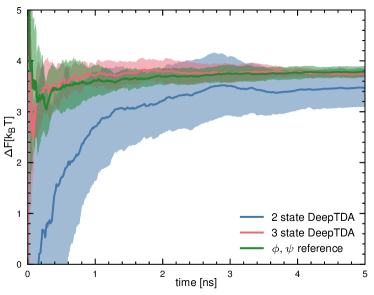
Figure 5: Free energy difference between the $C_{7eq}$ and $C_{ax}$ basins of alanine dipeptide over time. Shown are the results obtained from 5 independent enhanced sampling simulations respectively, biasing the 2-state and 3-state DeepTDA CV, as well as reference calculation using the dihedral angles $\phi,\psi$ as CV.

Conclusions

We have presented an iterative approach based on the metadynamics of paths algorithm [1] to reconstruct free energy landscapes as a function of data-driven CVs using datasets supplemented with configurations from the transition state ensemble. In doing so, we have also addressed directly the problem of designing efficient CVs in trajectory space. We found that the augmentation with MoP data leads to a significant performance increase of the learned CVs in configurational space. Good CVs could be generated even when using MoP in an exploratory manner (i.e., convergence was not needed), thus considerably reducing the computational effort required to obtain meaningful results.

Besides being the only path sampling method so far enabling the exploration of free energy landscapes using CVs, the use of MoP to obtain transition state data offers several other advantages: (i) in contrast to other path sampling methods [27, 34, 25, 24], MoP enables the sampling of (non)reactive trajectories in an unconstrained manner and is robust to the choice of sub-optimal CVs; (ii) running MoP amounts to a single metadynamics simulation, considerably simplifying the methodology compared to Monte Carlo approaches like transition path sampling; (iii) MoP can be implemented in an extremely parallel fashion [39] to exploit modern massively parallel supercomputers (which have recently breached the exascale limit).

The efficiency of our procedure was tested in two models of increasing complexity, including a simple molecular system. We expect our protocol to aid in the discovery of collective variables, the exploration of transition pathways, and the estimation of free energy profiles in complex systems of relevance in biology, chemistry, and materials science. Future work will focus on scaling the proposed protocol to more challenging, real-world applications.

Finally, we note that, in this work, we have focused on building ML CVs that use only the spatial distribution of the samples obtained from MoP data. However, learning dynamical information from the trajectory data [19, 40, 20] is another very appealing avenue, as the sampled paths carry information on the unbiased dynamics of the system.

Data Availability

The input files for LAMMPS and PLUMED used to generate the presented results, scripts to compile the necessary software, as well as example code to train the DeepTDA NN CVs, can be found on GitHub at https://github.com/lmuellender/MoP-DeepTDA.

Funding

This research was partly supported by European Union’s HORIZON MSCA Doctoral Networks programme, under Grant Agreement No. 101072344, project AQTIVATE (Advanced computing, QuanTum algorIthms and data-driVen Approaches for science, Technology and Engineering). Furhtermore, the authors acknowledge support from the Helmholtz European Partnering program (“Innovative high-performance computing approaches for molecular neuromedicine”) and the Swedish eScience Research Center. The authors also gratefully acknowledge the Gauss Centre for Supercomputing e.V. (www.gauss-centre.eu) for funding this project by providing computing time through the John von Neumann Institute for Computing (NIC) on the GCS Supercomputer JUWELS [41] at Jülich Supercomputing Centre (JSC).

Supporting Information

DeepTDA CVs

The DeepTDA neural network CVs [35] are trained in PyTorch using an existing implementation in the mlcolvar package [42], in its release v0.2.0. The networks use a feed-forward architecture with 3 hidden layers with $\{24,12,1\}$ nodes and the ReLU activation function. To enforce the target distribution on the latent CV space, the objective function for the neural network is chosen to be a mean-squared error between the mean and standard deviation at the hidden layer and their respective target values, $\mu_{tg}$ and $\sigma_{tg}$, which in the one-dimensional case is given by,

$$L=\sum_{k}^{N_{s}}\alpha(\mu_{k}-\mu_{k}^{tg})^{2}+(\sigma_{k}-\sigma_{k}^{tg})^{2},$$ (4)

where $k$ denotes the $N_{s}$ different states, and the hyperparameters $\alpha$ and $\beta$ ensuring adequate scaling of the respective loss terms. The resulting DeepTDA CV is normalized over the training data to a range of $-1\leq s\leq 1$.
In all trained networks, the parameters are optimized using the ADAM optimizer [43] with a learning rate of $10^{-3}$. In addition to the TDA loss in equation 4, L2 regularization with $\lambda=10^{-5}$ has been added to the weights. The training is stopped when convergence of the loss function is reached, using an Early-Stopping routine with patience set to 15 epochs to avoid overfitting. The hyperparameters $\alpha$ and $\beta$ were set to values of $1$ and $250$, respectively. For the implementation details specific to the test systems described below, including the selection of training data from the simulated trajectories, the reader is referred to the supporting information.

Two-Dimensional Model Potential

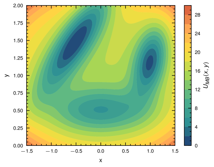
Figure S1: Isolines of the 2D model potential energy surface.

To evaluate the proposed methodology, we designed a two-dimensional model potential, based on the analytical form introduced by Müller and Brown [36]. The isolines of this modified potential are shown in Fig. S1, and has the analytical from

$$\begin{split}U_{\text{MB}}(x,y)&=\sum_{k}A_{k}\exp\left[a_{k}(x-x_{k}^{0})^{2}\right.\\ &\left.\quad+b_{k}(x-x_{k}^{0})(y-y_{k}^{0})+c_{k}(y-y_{k}^{0})^{2}\right],\\ \mathbf{A}&=(-16,-11,-17,2),\\ \mathbf{a}&=(-10,-1,-6.5,0.4),\\ \mathbf{b}&=(5,0,11,0),\\ \mathbf{c}&=(-5,-10,-6.5,1.1),\\ \mathbf{x}_{0}&=(1,0,-0.5,0),\\ \mathbf{y}_{0}&=(1.2,0.5,1.5,1).\end{split}$$ (5)

All simulations in this work are started in basin A, where the potential assumes its global minimum. In this work, we consider Langevin dynamics of a single particle moving along the model potential. The simulations use natural units, such that $k_{B}=1$, and a temperature of $T=0.1$, placing the highest free energy barrier at around $120\,k_{B}T$.
Because the analytical form of the potential is known, the difference in free energy between the basins A and C can be calculated directly via numerical integration, with

$$\Delta F=-\frac{1}{\beta}\log\frac{\int_{C}e^{-\beta U_{\text{MB}}(x,y)}dx\,dy}{\int_{A}e^{-\beta U_{\text{MB}}(x,y)}dx\,dy}$$ (6)

where $A=\{(x,y)\mid y>x+1.5\}$ and $C=\{(x,y)\mid x-1.5<y<x+1.5\}$, which in this case equates to $12.15\,k_{B}T$.

The simulations in configurational space of the 2D model potential were performed using the molecular simulation engine LAMMPS [44] in its stable release version from 23. June 2022, patched with PLUMED 2.8 [45], which also provides an interface with the LibTorch C++ library to implement the neural network-based DeepTDA CVs [42]. The damping constant in the Langevin thermostat is set to a value of $0.1$, which corresponds to a value of $\nu=10$, and the time step is set to $\Delta t=0.01$ in arbitrary units of time.
To perform enhanced sampling simulations we here use the recently introduced OPES method [11], an implementation for which is provided in PLUMED. For detailed information about the usage of this bias potential and a definition of the relevant parameters, the reader is referred to the PLUMED documentation. For the OPES simulation with the initial 2-state DeepTDA CV, the parameters are set to BARRIER $=17$, PACE $=300$ and SIGMA $=0.03$. The SIGMA is chosen to reflect the standard deviation of the CV values in a short, unbiased simulation. For OPES simulation using the 4-state DeepTDA CV, the parameter values BARRIER $=15$, PACE $=300$ and SIGMA $=0.01$. The SIGMA parameter is again chosen as the CVs standard deviation in unbiased simulation, and the BARRIER parameter is lowered to allow for faster convergence.

To carry out the Metadynamics of Paths simulations in trajectory space, an extra fix is added to the LAMMPS suite, adapted from Ref. [1] to directly evaluate the analytical derivatives of the potential. The friction and time step parameter of the polymer are set to $\nu=10$ and $\Delta t=0.01$, respectively. In trajectory space, the polymers, made up of $N=288$ beads, are then sampled at a time step of $0.01$ and a damping constant of damp $=100$. The initial configuration for the polymer was obtained by running an unbiased MetaD of Paths simulation starting from the same configuration for every bead at $\mathbf{r}=(-0.5,1.5)^{\intercal}$ and letting the polymer relax for $10^{4}$ steps.
To enhance the sampling of the polymers, OPES is again used. The underlying configurational DeepTDA CV is first evaluated on each bead. Then, a modified version of the CUSTOM/MATHEVAL action is used to access the values from different beads, to evaluate the end-to-end difference for use as the trajectory CV. MoP simulations with both the initial DeepTDA CV and the 4-state CV are performed with OPES parameters set to BARRIER $=20$ and PACE $=500$, and an adaptive SIGMA.

DeepTDA CV Training for 2D Model Potential

For the initial DeepTDA CV $s_{0}$ on the unbiased training data, the target centers and widths are chosen as $\mu_{tg}=[-7,7]$ and $\sigma_{tg}=[0.2,0.2]$, respectively. The training data set consists of 6000 configurations from each of the initial metastable states, as shown labeled ’unbiased data’ in Fig. S2b.
We now train the 4-state DeepTDA CV in a two-step process, the reason for which is explained below. From the trajectory data, shown in Fig. 2e, we first isolate the reactive trajectories and those trapped in metastable states. This can be quantified by using the trajectory CV $S(\{\mathbf{R}_{i}\})$ in Eq. 3, and we here classify as kinetically trapped or confined trajectories with values of $S\leq 0.3$. In this way, we find trajectories trapped in the initial basin A, but also those confined to the previously ’unknown’ basin B. To separate these configurations between known and unknown states, OPTICS clustering [46] is used.
To filter the reactive trajectories, the range of values to select for depends strongly on the respective system under consideration, and how well the initial DeepTDA CV is able to discern different regions of the phase space, which is why we first train a 3-state DeepTDA CV $s_{1}$. For the training of this CV, target centers and widths for this CV are chosen as $\mu_{tg}=[-15,0,15]$ and $\sigma=[0.3,1.0,0.3]$ respectively, corresponding to a respective separation of $\Delta=15$. Evaluating this CV on the previously obtained trajectory data, we can now much more confidently set a threshold of $\absolutevalue{S\{\mathbf{R}_{i}\}}\geq 1$ to select trajectories that connect A and B. Now, information from the reactive paths is taken into account, by selecting configurations that satisfy $\mu_{A}+3\sigma_{A}\leq s_{1}(\mathbf{r})\leq\mu_{int}-3\sigma_{int}$, where the $\mu_{A/int}$ and $\sigma_{A/int}$ denote mean and standard deviation in the initial/intermediate metastable states, respectively. The precise multiple of the standard deviation should be chosen carefully, as to select data that covers as wide a CV_c range as possible, without introducing overlaps. This data is added as a fourth state for the training of the 4-state DeepTDA CV $s_{2}$, using the target widths $\mu_{tg}=[-30,-15,0,15]$ and centers $\sigma_{tg}=[0.3,4.0,1.0,0.3]$, and the training data is shown in Fig. S2a. These values are chosen by visual inspection of the CV histograms in the training data, to select for sharp peaks in the metastable states and broader, slightly overlapping distributions for the reactive paths and transition states (see Fig. S2b). In both cases, a random subset of 6000 configurations is selected from the trapped and reactive trajectory data, to match the amount of unbiased data.

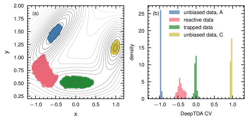
Figure S2: Training data and histogram of CV distributions for training the 4-state DeepTDA CV in the case of the 2D model potential. (a) Scatter plot of the training data, with data from unbiased simulations in the left and right basins shown respectively in blue and yellow, selected configurations from reactive paths generated by MoP shown in pink and configurations from trapped paths in the intermediate basin shown in green. From all 4 states, 6666 configurations are shown and used to train the 4-state DeepTDA CV. Isolines of the 2D model potential are indicated in grey. (b) Histogram of the trained 4-state DeepTDA CV evaluated on the training data from the different basins. Note how the unbiased data are mapped to sharp peaks at the end points, and data from reactive and confined trajectories are mapped to broader distributions.

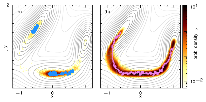
Figure S4: Trapped (a) and reactive (b) trajectories, isolated from a MoP simulation using the 4-state DeepTDA CV for the 2D model potential in trajectory space. The densities are calculated from 208 trapped and 2603 reactive trajectories, respectively. Examples of trapped trajectories are shown in blue. Reactive trajectories connecting the basins A-B, A-C and B-C are shown in green, pink and red, respectively. Isolines of the potential are indicated in grey.

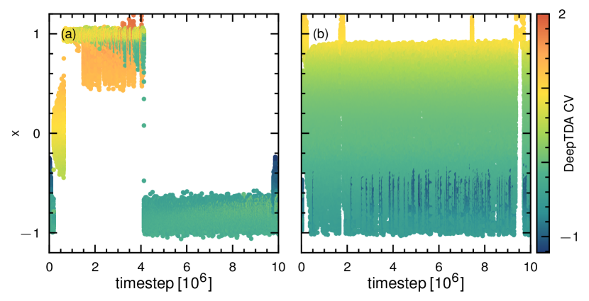
Figure S6: Time evolution of the x coordinate of the 2D model potential, during biased simulations in configurational space using the (a) 2-state and (b) 4-state DeepTDA CVs, colored according to respective CV value.

Alanine Dipeptide

For the simulations of the conformational dynamics of alanine dipeptide in vacuum, we again used LAMMPS patched with PLUMED. The Amber99-SB [47] force field was used, converted for use in LAMMPS using the convert.py script in the InterMol [48] software. We consider Langevin dynamics in an NVE ensemble at a temperature of 300 K, and use a time step of 0.5 fs and a dampening constant of 500 fs. To perform biased simulations with the DeepTDA CVs in OPES, we used parameter values BARRIER $=50$, PACE $=100$, and an adaptive SIGMA.

To carry out MoP simulations, we used the path_dynamics fix provided by and described in Ref. [1]. The parameters of the polymer are set to $\nu=0.25\frac{1}{s}$ and $\Delta t=1fs$. In trajectory space, the polymers, made up of $N=512$ beads, are then sampled at a time step of $1.0$ and a damping constant of damp $=1000$ in trajectory space. The initial configuration for the polymer was obtained by running an unbiased MoP simulation starting from the same configuration in the $C_{5}$ basin for every bead and letting the polymer relax for $10^{6}$ steps. As described above, we again use OPES to drive the sampling of the polymers with a bias potential, using parameter values BARRIER $=80$ and PACE $=1000$, as well as a bias factor of 15.

The DeepTDA neural network-CVs for Alanine Dipeptide are trained with largely identical settings to the case of the model potential, with the exception of a learning rate of $10^{-3}$. As a set of descriptors, we use the set of pairwise distances between the heavy atoms of alanine dipeptide, as compiled by Bonati and coworkers [18], thereby insuring rototranslational invariance of our CV.
The 2-state DeepTDA CV $s_{0}$ is trained with 4000 configurations each from the $C_{5}/C_{7eq}$ and $C_{ax}$ basins, respectively. As values for the target centers and widths for the modes in CV spaces, we again choose $\mu_{tg}=[-7,7]$ and $\sigma_{tg}=[0.2,0.2]$. Proceeding as described in the main text, by first separating the trajectory data, sampled with MoP using the 2-state CV, into trapped paths with a value of $S(\{\mathbf{R}_{i}\})\leq 0.5$ and reactive paths with $S(\{\mathbf{R}_{i}\})\geq 1.2$. In this case, we don’t observe any confined data in previously unexplored regions, so we proceed by integrating data from the transition state as an intermediary. The training data for the 3-state DeepTDA CV $s_{1}$ is thus chosen by selecting configurations with $s_{0}\geq 0.3$ from the reactive paths, as shown in Fig. S7. From this data, we again choose a random subset of 4000 configurations to match the amount of unbiased data, and train the new CV by choosing target centers and widths $\mu_{tg}=[-7,0,7]$ and $\sigma=[0.3,1.0,0.3]$.

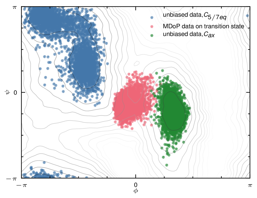
Figure S7: Training data for the 3-state DeepTDA CV in the case of alanine dipeptide. Scatter plot of the training data, with data from unbiased simulations in the C_5,7eq and C_ax basins shown respectively in blue and green, and selected configurations from reactive paths generated by MoP shown in pink. From all 3 states, 4000 configurations are shown and used to train the 3-state DeepTDA CV. Isolines of the FES calculated from a converged reference calculation using the $\phi,\psi$ dihedral angles are indicated in grey.

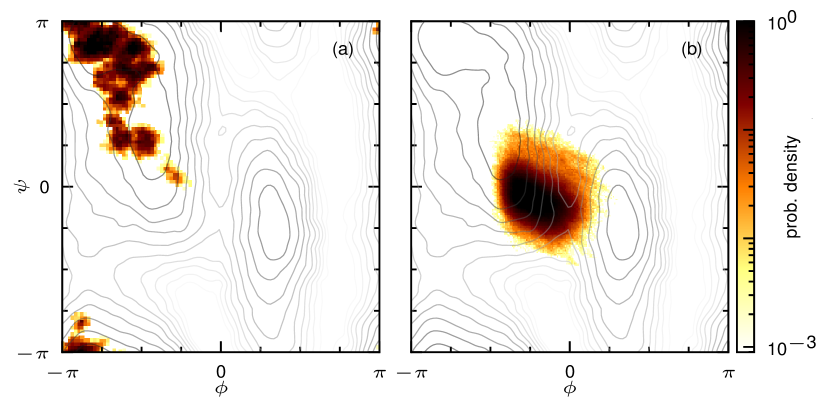
Figure S8: Trapped (a) and reactive (b) trajectories, isolated from a MoP simulation using the 2-state DeepTDA CV for alanine dipeptide in trajectory space. The normalized densities are calculated from 125 trapped and 3529 reactive trajectories, respectively. Isolines of the FES of alanine dipeptide calculated from a converged reference calculation using the $\phi,\psi$ dihedral angles are indicated in grey.

Figure S10: Time evolution during biased simulations in configurational space using the (a) 2-state and (b) 3-state DeepTDA CVs, colored according to respective CV value.

References

- [1] Davide Mandelli, Barak Hirshberg and Michele Parrinello “Metadynamics of Paths” In Physical Review Letters 125.2 American Physical Society, 2020, pp. 026001 DOI: 10.1103/PhysRevLett.125.026001
- [2] Jérôme Hénin et al. “Enhanced Sampling Methods for Molecular Dynamics Simulations [Article v1.0]” In Living Journal of Computational Molecular Science 4.1, 2022, pp. 1583–1583 DOI: 10.33011/livecoms.4.1.1583
- [3] Omar Valsson, Pratyush Tiwary and Michele Parrinello “Enhancing Important Fluctuations: Rare Events and Metadynamics from a Conceptual Viewpoint” In Annual Review of Physical Chemistry 67.1, 2016, pp. 159–184 DOI: 10.1146/annurev-physchem-040215-112229
- [4] Lucie Delemotte et al. “Free-Energy Landscape of Ion-Channel Voltage-Sensor–Domain Activation” In Proceedings of the National Academy of Sciences 112.1 Proceedings of the National Academy of Sciences, 2015, pp. 124–129 DOI: 10.1073/pnas.1416959112
- [5] Pratyush Tiwary, Vittorio Limongelli, Matteo Salvalaglio and Michele Parrinello “Kinetics of Protein–Ligand Unbinding: Predicting Pathways, Rates, and Rate-Limiting Steps” In Proceedings of the National Academy of Sciences 112.5 Proceedings of the National Academy of Sciences, 2015, pp. E386–E391 DOI: 10.1073/pnas.1424461112
- [6] Ronald Blaak, Stefan Auer, Daan Frenkel and Hartmut Löwen “Crystal Nucleation of Colloidal Suspensions under Shear” In Physical Review Letters 93.6, 2004, pp. 068303 DOI: 10.1103/PhysRevLett.93.068303
- [7] G.M. Torrie and J.P. Valleau “Nonphysical Sampling Distributions in Monte Carlo Free-Energy Estimation: Umbrella Sampling” In Journal of Computational Physics 23.2, 1977, pp. 187–199 DOI: 10.1016/0021-9991(77)90121-8
- [8] Arthur F. Voter “Hyperdynamics: Accelerated Molecular Dynamics of Infrequent Events” In Physical Review Letters 78.20, 1997, pp. 3908–3911 DOI: 10.1103/PhysRevLett.78.3908
- [9] Alessandro Laio and Michele Parrinello “Escaping Free-Energy Minima” In Proceedings of the National Academy of Sciences 99.20 Proceedings of the National Academy of Sciences, 2002, pp. 12562–12566 DOI: 10.1073/pnas.202427399
- [10] Alessandro Barducci, Giovanni Bussi and Michele Parrinello “Well-Tempered Metadynamics: A Smoothly Converging and Tunable Free-Energy Method” In Physical Review Letters 100.2 American Physical Society, 2008, pp. 020603 DOI: 10.1103/PhysRevLett.100.020603
- [11] Michele Invernizzi and Michele Parrinello “Rethinking Metadynamics: From Bias Potentials to Probability Distributions” In J. Phys. Chem. Lett., 2020, pp. 6
- [12] Eric Darve, David Rodríguez-Gómez and Andrew Pohorille “Adaptive Biasing Force Method for Scalar and Vector Free Energy Calculations” In The Journal of Chemical Physics 128.14, 2008, pp. 144120 DOI: 10.1063/1.2829861
- [13] Omar Valsson and Michele Parrinello “Variational Approach to Enhanced Sampling and Free Energy Calculations” In Physical Review Letters 113.9 American Physical Society, 2014, pp. 090601 DOI: 10.1103/PhysRevLett.113.090601
- [14] K. Lindorff-Larsen, S. Piana, R.. Dror and D.. Shaw “How Fast-Folding Proteins Fold” In Science 334.6055, 2011, pp. 517–520 DOI: 10.1126/science.1208351
- [15] Giulia Sormani, Alex Rodriguez and Alessandro Laio “Explicit Characterization of the Free-Energy Landscape of a Protein in the Space of All Its C Carbons” In Journal of Chemical Theory and Computation 16.1, 2020, pp. 80–87 DOI: 10.1021/acs.jctc.9b00800
- [16] Ming Chen “Collective Variable-Based Enhanced Sampling and Machine Learning” In The European Physical Journal B 94.10, 2021, pp. 211 DOI: 10.1140/epjb/s10051-021-00220-w
- [17] Dan Mendels, GiovanniMaria Piccini and Michele Parrinello “Collective Variables from Local Fluctuations” In The Journal of Physical Chemistry Letters 9.11, 2018, pp. 2776–2781 DOI: 10.1021/acs.jpclett.8b00733
- [18] Luigi Bonati, Valerio Rizzi and Michele Parrinello “Data-Driven Collective Variables for Enhanced Sampling” In The Journal of Physical Chemistry Letters 11.8, 2020, pp. 2998–3004 DOI: 10.1021/acs.jpclett.0c00535
- [19] Guillermo Pérez-Hernández et al. “Identification of Slow Molecular Order Parameters for Markov Model Construction” In The Journal of Chemical Physics 139.1, 2013, pp. 015102 DOI: 10.1063/1.4811489
- [20] Luigi Bonati, GiovanniMaria Piccini and Michele Parrinello “Deep Learning the Slow Modes for Rare Events Sampling” In Proceedings of the National Academy of Sciences 118.44, 2021, pp. e2113533118 DOI: 10.1073/pnas.2113533118
- [21] Wei Chen and Andrew L. Ferguson “Molecular Enhanced Sampling with Autoencoders: On-the-fly Collective Variable Discovery and Accelerated Free Energy Landscape Exploration” In Journal of Computational Chemistry 39.25, 2018, pp. 2079–2102 DOI: 10.1002/jcc.25520
- [22] Mohammad M. Sultan and Vijay S. Pande “Automated Design of Collective Variables Using Supervised Machine Learning” In The Journal of Chemical Physics 149.9, 2018, pp. 094106 DOI: 10.1063/1.5029972
- [23] João Marcelo Lamim Ribeiro, Pablo Bravo, Yihang Wang and Pratyush Tiwary “Reweighted Autoencoded Variational Bayes for Enhanced Sampling (RAVE)” In The Journal of Chemical Physics 149.7, 2018, pp. 072301 DOI: 10.1063/1.5025487
- [24] Lixin Sun et al. “Multitask Machine Learning of Collective Variables for Enhanced Sampling of Rare Events” In Journal of Chemical Theory and Computation 18.4, 2022, pp. 2341–2353 DOI: 10.1021/acs.jctc.1c00143
- [25] Ferry Hooft, Alberto Pérez de Alba Ortíz and Bernd Ensing “Discovering Collective Variables of Molecular Transitions via Genetic Algorithms and Neural Networks” In Journal of Chemical Theory and Computation 17.4, 2021, pp. 2294–2306 DOI: 10.1021/acs.jctc.0c00981
- [26] Mary A. Rohrdanz, Wenwei Zheng and Cecilia Clementi “Discovering Mountain Passes via Torchlight: Methods for the Definition of Reaction Coordinates and Pathways in Complex Macromolecular Reactions” In Annual Review of Physical Chemistry 64.1, 2013, pp. 295–316 DOI: 10.1146/annurev-physchem-040412-110006
- [27] Dhiman Ray, Enrico Trizio and Michele Parrinello “Deep Learning Collective Variables from Transition Path Ensemble” In The Journal of Chemical Physics 158.20, 2023, pp. 204102 DOI: 10.1063/5.0148872
- [28] L. Onsager and S. Machlup “Fluctuations and Irreversible Processes” In Physical Review 91.6, 1953, pp. 1505–1512 DOI: 10.1103/PhysRev.91.1505
- [29] Lawrence R. Pratt “A Statistical Method for Identifying Transition States in High Dimensional Problems” In The Journal of Chemical Physics 85.9, 1986, pp. 5045–5048 DOI: 10.1063/1.451695
- [30] D. Mandelli and M. Parrinello “A Modified Nudged Elastic Band Algorithm with Adaptive Spring Lengths” In The Journal of Chemical Physics 155.7, 2021, pp. 074103 DOI: 10.1063/5.0059593
- [31] Christoph Dellago, Peter G. Bolhuis, Félix S. Csajka and David Chandler “Transition Path Sampling and the Calculation of Rate Constants” In The Journal of Chemical Physics 108.5, 1998, pp. 1964–1977 DOI: 10.1063/1.475562
- [32] Peter G. Bolhuis, David Chandler, Christoph Dellago and Phillip L. Geissler “Transition Path Sampling: Throwing Ropes Over Rough Mountain Passes, in the Dark” In Annual Review of Physical Chemistry 53.1, 2002, pp. 291–318 DOI: 10.1146/annurev.physchem.53.082301.113146
- [33] Ao Ma and Aaron R. Dinner “Automatic Method for Identifying Reaction Coordinates in Complex Systems” In The Journal of Physical Chemistry B 109.14, 2005, pp. 6769–6779 DOI: 10.1021/jp045546c
- [34] Robert B. Best and Gerhard Hummer “Reaction Coordinates and Rates from Transition Paths” In Proceedings of the National Academy of Sciences 102.19, 2005, pp. 6732–6737 DOI: 10.1073/pnas.0408098102
- [35] Enrico Trizio and Michele Parrinello “From Enhanced Sampling to Reaction Profiles” In The Journal of Physical Chemistry Letters 12.35, 2021, pp. 8621–8626 DOI: 10.1021/acs.jpclett.1c02317
- [36] Klaus Müller and Leo D. Brown “Location of Saddle Points and Minimum Energy Paths by a Constrained Simplex Optimization Procedure” In Theoretica Chimica Acta 53.1, 1979, pp. 75–93 DOI: 10.1007/BF00547608
- [37] Michele Invernizzi and Michele Parrinello “Exploration vs Convergence Speed in Adaptive-Bias Enhanced Sampling” In Journal of Chemical Theory and Computation 18.6 American Chemical Society, 2022, pp. 3988–3996 DOI: 10.1021/acs.jctc.2c00152
- [38] Rubicelia Vargas, Jorge Garza, Benjamin P. Hay and David A. Dixon “Conformational Study of the Alanine Dipeptide at the MP2 and DFT Levels” In The Journal of Physical Chemistry A 106.13, 2002, pp. 3213–3218 DOI: 10.1021/jp013952f
- [39] August Calhoun, Marc Pavese and Gregory A. Voth “Hyper-Parallel Algorithms for Centroid Molecular Dynamics: Application to Liquid Para-Hydrogen” In Chemical Physics Letters 262.3-4, 1996, pp. 415–420 DOI: 10.1016/0009-2614(96)01109-8
- [40] Christoph Wehmeyer and Frank Noé “Time-Lagged Autoencoders: Deep Learning of Slow Collective Variables for Molecular Kinetics” In The Journal of Chemical Physics 148.24, 2018, pp. 241703 DOI: 10.1063/1.5011399
- [41] Jülich Supercomputing Centre “JUWELS Cluster and Booster: Exascale Pathfinder with Modular Supercomputing Architecture at Juelich Supercomputing Centre” In Journal of large-scale Research Facilities 7.A138, 2021 DOI: 10.17815/jlsrf-7-183
- [42] Luigi Bonati, Enrico Trizio, Andrea Rizzi and Michele Parrinello “A Unified Framework for Machine Learning Collective Variables for Enhanced Sampling Simulations: Mlcolvar” In The Journal of Chemical Physics 159.1, 2023, pp. 014801 DOI: 10.1063/5.0156343
- [43] Diederik P. Kingma and Jimmy Ba “Adam: A Method for Stochastic Optimization” arXiv, 2017 arXiv:1412.6980
- [44] Aidan P. Thompson et al. “LAMMPS - a Flexible Simulation Tool for Particle-Based Materials Modeling at the Atomic, Meso, and Continuum Scales” In Computer Physics Communications 271, 2022, pp. 108171 DOI: 10.1016/j.cpc.2021.108171
- [45] Gareth A. Tribello et al. “PLUMED 2: New Feathers for an Old Bird” In Computer Physics Communications 185.2, 2014, pp. 604–613 DOI: 10.1016/j.cpc.2013.09.018
- [46] Mihael Ankerst, Markus M. Breunig, Hans-Peter Kriegel and Jörg Sander “OPTICS: Ordering Points to Identify the Clustering Structure” In ACM SIGMOD Record 28.2, 1999, pp. 49–60 DOI: 10.1145/304181.304187
- [47] Viktor Hornak et al. “Comparison of Multiple Amber Force Fields and Development of Improved Protein Backbone Parameters” In Proteins: Structure, Function, and Bioinformatics 65.3, 2006, pp. 712–725 DOI: 10.1002/prot.21123
- [48] Michael R. Shirts et al. “Lessons Learned from Comparing Molecular Dynamics Engines on the SAMPL5 Dataset” In Journal of Computer-Aided Molecular Design 31.1, 2017, pp. 147–161 DOI: 10.1007/s10822-016-9977-1