High-Performance Transformers for Table Structure Recognition Need Early Convolutions

Abstract

tsr aims to convert tabular images into a machine-readable format, where a visual encoder extracts image features and a textual decoder generates table-representing tokens. Existing approaches use classic convolutional neural network (CNN) backbones for the visual encoder and transformers for the textual decoder. However, this hybrid CNN-Transformer architecture introduces a complex visual encoder that accounts for nearly half of the total model parameters, markedly reduces both training and inference speed, and hinders the potential for self-supervised learning in table structure recognition (TSR). In this work, we design a lightweight visual encoder for TSR without sacrificing expressive power. We discover that a convolutional stem can match classic CNN backbone performance, with a much simpler model. The convolutional stem strikes an optimal balance between two crucial factors for high-performance TSR: a higher receptive field (RF) ratio and a longer sequence length. This allows it to “see” an appropriate portion of the table and “store” the complex table structure within sufficient context length for the subsequent transformer. We conducted reproducible ablation studies and open-sourced our code at https://github.com/poloclub/tsr-convstem to enhance transparency, inspire innovations, and facilitate fair comparisons in our domain as tables are a promising modality for representation learning.

1 Introduction

tsr aims to extract both the structure and cell data of a tabular image into a machine-readable format [1, 2, 3]. This task is inherently an image-to-text generation problem, where a visual encoder extracts image features, and a textual decoder generates tokens representing the table, typically in HTML [4] or LaTeX symbols [5]. In the existing literature, the visual encoder often employs classic CNN backbones, e.g., ResNets and their variants [6], and the textural decoder consists of a stack of transformer encoders and decoders [7]. However, this hybrid CNN-transformer architecture introduces a complex visual encoder that takes up almost half of the total model parameters and significantly reduces both training and inference speed [8, 9, 10]. Dosovitskiy, et al. [11] compared the vanilla vision Transformer (ViT), which used a simple linear projection, with the “hybrid ViT” that used 40 convolution layers (most of a ResNet-50) and found that both models performed similarly for image classification tasks. Furthermore, linear projection has proven to be a powerful visual processor, enabling self-supervised learning (SSL) in related domains, e.g., document image classification and layout analysis tasks [12, 13]. This leads us to ponder: How to simplify the visual encoder for TSR while reducing computational costs without sacrificing performance? Can we simply employ the aforementioned linear projection?

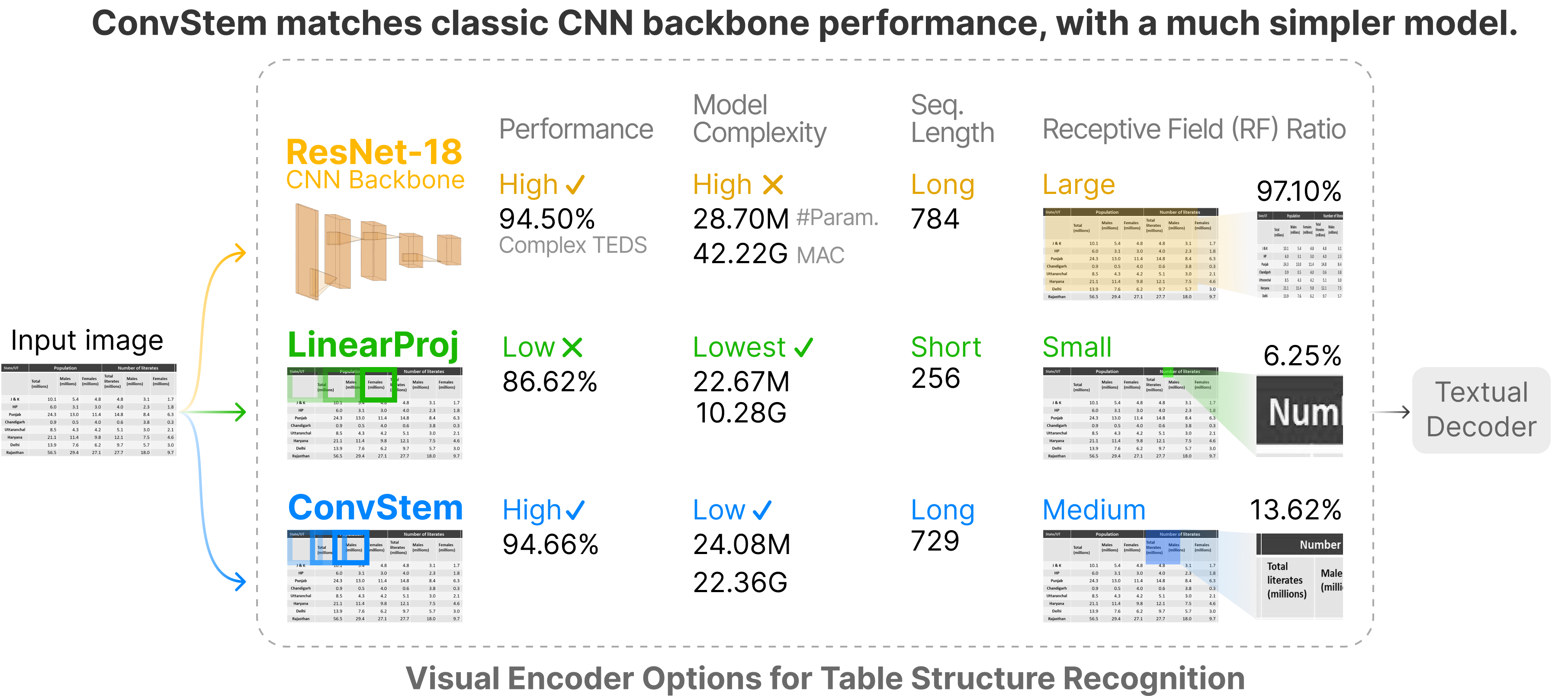
Figure 1: Using convolutional stem (ConvStem) in a visual encoder for table structure recognition (TSR) achieves performance comparable to that of a CNN backbone while significantly reducing model complexity. The CNN backbone is performant with large RF but exhibits high model complexity. Linear projection is the simplest but suffers in terms of performance due to limited RF and sequence length. In contrast, ConvStem strikes an optimal balance between two crucial factors for high-performance TSR: a higher receptive field (RF) ratio and a longer sequence length. We illustrate each visual encoder option’s RF (zoomed in) and compute its RF ratio. Using the image features extracted from the visual encoder, a textual decoder then generates tokens representing the table.

We address the above research questions and make the following major contributions (Fig. 1):

1. We discover that a convolutional stem can match classic CNN backbone performance, with a much simpler model (Fig. 1: bottom). This discovery stems from our motivation to design a lightweight visual encoder for TSR without compromising on expressive power. To achieve this, we began by replacing the CNN backbone with ViT’s linear projection. However, this substitution led to a noticeable $\sim 6$ percentage points (pp) decrease in overall accuracy and $\sim 8$ pp for complex tables. The major difference between the CNN backbone and the linear projection lies in the total number of convolution layers. A standard ResNet-18 has 17 convolution layers, whereas the linear projection only has one. Evidence shows that incorporating a few early convolutions is crucial to balance inductive biases and the representation learning ability of transformers [14]. We therefore reintroduce a few convolution layers by constructing the convolutional stem (Sec. 3.2). This addition proves highly effective, bridging the performance gap between the linear projection and the CNN backbone while still achieving low model complexity.

2. The convolutional stem strikes an optimal balance between two crucial factors for high-performance TSR: a higher receptive field (RF) ratio and a longer sequence length. The RF ratio, defined as the ratio of the RF in the input to the size of the entire input, reflects how much of an input impacts the visual encoder’s output. As illustrated in Fig. 1, a small RF ratio provides minimal structural information, while a medium-sized one offers ample context and distinguishable features. Sequence length refers to the transformer’s input length, and longer context during training typically yields higher-quality models [15]. Consequently, the performance of linear projection is capped since the RF ratio and the sequence length are inversely correlated, i.e., an increase in the RF ratio means a larger patch size, resulting in a shorter sequence. In contrast, the convolutional stem independently balances these two factors, increasing the RF ratio while maintaining the sequence length. This enables it to “see” an appropriate portion of the table and “store” the complex table structure within sufficient context length for the subsequent transformer. Additionally, with fewer convolutional layers than a typical CNN backbone, the convolutional stem significantly reduces model complexity.

3. Reproducible research and open-source code. We provide all the details regarding training, validation, and testing, which include model architecture configurations, model complexities, dataset information, evaluation metrics, training optimizer, learning rate, and ablation studies. Our work is open source and publicly available at https://github.com/poloclub/tsr-convstem. We believe that reproducible research and open-source code enhance transparency, inspire state-of-the-art (SOTA) innovations, and facilitate fair comparisons in our domain as tables are a promising modality for representation learning.

2 Related Work

TSR based on image-to-text generation. This method treats the table structure as a sequence and adopts an end-to-end image-to-text paradigm. Deng, et al. [16] employed a hybrid CNN-LSTM architecture to generate the LaTeX code of the table. Zhong, et al. [1] introduced an encoder-dual-decoder (EDD) architecture in which two RNN-based decoders were responsible for logical and cell content, respectively. Both TableFormer [2] and TableMaster [5] enhanced the EDD decoder with a transformer decoder and included a regression decoder to predict the bounding box instead of the content. VAST [3] took a different approach by modeling the bounding box coordinates as a language sequence and proposed an auxiliary visual alignment loss to ensure that the logical representation of the non-empty cells contains more local visual details. Our goal differs from existing approaches as we focused on designing a lightweight visual encoder and conducting a comprehensive comparison of three different types of visual encoders through ablation studies.

Applications of lightweight visual encoders While the transformer has become the solid mainstream for natural language processing (NLP) tasks, its applications in computer vision remained limited until the advent of ViT [11]. For visual tasks, attention mechanisms were either applied in conjunction with CNNs [17] or used to replace components within CNNs [18]. vit demonstrated that this reliance on CNNs is unnecessary and transformers can directly process sequences of image patches through linear projection. This same simplification also occurred in the vision-language pretraining (VLP) domain, where early models used severely slow region selection [8] or grid features [10]. vilt [19] adopted the same linear projection from ViT to minimize overhead in the visual encoder. The convolutional stem [14], another lightweight visual encoder, reintroduced minimal convolutions to enhance optimization stability and improve peak performance and robustness [20, 21]. It was initially introduced to replace the linear projection in ViTs, serving as the earliest stage of input image processing [14]. Lightweight visual encoders are not only used in supervised learning described above but also in SSL. BEiT [13] designed a masked image modeling task to pretrain vision transformers. Specifically, each image has two views: image patches from linear projection and visual tokens. The pretraining objective is to recover the original visual tokens based on the corrupted image patches. Inspired by BEiT, DiT [12] proposed a self-supervised pre-trained document image Transformer model, which leveraged large-scale unlabeled document images for pre-training. Hence, the lightweight visual encoder is a powerful input image processor. In this work, we explore these lightweight visual encoders in TSR for the first time.

3 Discovering Visual Encoder Impact on TSR Architecture

3.1 Overview of TSR Pipeline

The goal of TSR is to translate the input tabular image $I$ into a machine-readable sequence $T$. Specifically, $T$ includes table structure $T_{s}$ defined by HTML table tags and table content $T_{c}$ defined by standard NLP vocabulary. The prediction of $T_{c}$ is triggered when a non-empty table cell is encountered in $T_{s}$, e.g., <td> for a single cell or > for a spanning cell. If the corresponding portable document format (PDF) is provided, a cell coordinate decoder will predict the cell location and extract $T_{c}$ directly from the PDF, which is also triggered by a non-empty table cell. Thus, accurate structure prediction is a bottleneck that affects the performance of the downstream cell data recognition. Our model focuses on the table structure prediction and comprises two modules: visual encoder and textual decoder. The visual encoder extracts image features and the textual decoder generates HTML table tags based on the image features. Sec. 3.2 and 3.3 introduce the visual encoder and textual decoder and Sec. 3.4 presents the training loss function.

3.2 Comparing Visual Encoder Options

Given an input tabular image of size $(H,W)$, the visual encoder extracts the features required for downstream transformers. In this section, we compare three types of visual encoders: CNN backbones, linear projection, and convolutional stem.

CNN backbone. Among the architectures used in current TSR research, off-the-shelf CNN backbones, especially ResNets and ResNet variants [6] are the most widely employed. EDD [1] explored five different ResNet-18 variants, TableFormer [2] used a ResNet-18 with an additional adaptive pooling layer, and VAST [3] modified a ResNet-31 equipped with multi-aspect global content attention [22]. We use models from Torchvision libraries [23] and evaluate ResNet-18, ResNet-34, and ResNet-50. The penultimate pooling and final linear layers are removed and the output is the feature map from the last convolution layer. All ResNet-18, ResNet-34, and ResNet-50 downsample the input image by 16, thus the input sequence length for the transformer is $N=HW/16^{2}$. The receptive field of ResNet-18, ResNet-34, and ResNet-50 are 435, 899, and 427, respectively [24].

Linear projection. Cordonnier, et al. [25] initially introduced the concept of linear projection, and ViT [11] further demonstrated its scalability via large-scale pretraining. Building upon the simplicity of this design, vision-and-language transformer (ViLT) [19] modified the visual encoder by replacing the region supervision and the convolutional backbone with the linear projection. The modification significantly accelerated the inference speed, all while maintaining the model’s expressive power. The linear projection layer reshapes the image $I\in\mathbb{R}^{H\times W\times C}$ into a sequence of flattened 2D patches $I_{p}\in\mathbb{R}^{N\times(P^{2}\cdot C)}$, where $C$ is the number of channels, $(P,P)$ is the size of each image patch, and $N=HW/P^{2}$ is the number of patches, which is also the input sequence length for the transformer of the textual decoder. It is implemented by a stride $P$, kernel $P\times P$ convolution applied to the input image. The receptive field of the linear projection is the same as the patch size $P$. We denote “LinearProj-28” as a linear projection layer of $P=28$.

Convolutional stem. The convolutional stem was first introduced to replace the linear projection in ViTs, serving as the earliest stage of processing input image [14]. This early convolution enhances optimization stability and improves peak performance and robustness [20, 21]. To implement the convolutional stem, we employ a stack of stride 2, kernel $3\times 3$ convolutions, followed by a single stride 1, kernel $1\times 1$ convolution at the end to match the $d$–dimension feature of the transformer. We tune the receptive field of the convolutional stem by varying the kernel size, layers of convolutions, and input image size. Denote “ConvStem” as a visual encoder that uses convolutional stem as the CNN backbone.

3.3 Textual Decoder

The table structure can be defined either using HTML tags [4] or LaTeX symbols [5]. Since these different representations are convertible, we select HTML tags as they are the most commonly used format in dataset annotations [1, 26, 4]. Our HTML structural corpus has 32 tokens, including (1) starting tags <thead>, <tbody>, <tr>, <td>, along with their corresponding closing tags; (2) spanning tags <td, > with the maximum values for rowspan and colspan set at 10; (3) special tokens <sos>, <eos>, <pad>, and <unk>. The textual decoder is a stack of transformer encoder and decoder layers, primarily comprised of multi-head attention and feed-forward layers. During training, we apply the teacher forcing so that the transformer decoder receives ground truth tokens. At inference time, we employ greedy decoding, using previous predictions as input for the transformer decoder.

3.4 Loss Function

We formulate the training loss based on the language modeling task because the HTML table tags are predicted in an autoregressive manner. Denote the probability of the $i$th step prediction $p(t_{s_{i}}|I,t_{s_{1}:s_{i-1}};\theta)$, we directly maximize the correct structure prediction by using the following formulation:

$$\theta^{\ast}=\operatorname*{arg\ max}_{\theta}\sum_{(I,T_{s})}\log p(T_{s}|I;\theta),$$ (1)

where $\theta$ are the parameters of our model, $I$ is a tabular image, and $T_{s}$ is the correct structure sequence. According to language modeling, we apply the chain rule to model the joint probability over a sequence of length $n$ as

$$\log p(T_{s}|I;\theta)=\sum_{i=2}^{n}\log p(t_{s_{i}}|I,t_{s_{1}:s_{i-1}};\theta).$$ (2)

The start token $t_{s_{1}}$ is a fixed token <sos> in both training and testing.

4 Experiments

4.1 Settings

Architecture. The textual decoder has four layers of transformer decoders. For the visual encoder using the CNN backbone, we employ two layers of transformer encoder as this is shown to be the optimal setting [2]. For all other visual encoders, we use the same layers of transformer encoders and decoders [7]. All transformer layers have an input feature size of $d=512$, a feed-forward network of 1024, and 8 attention heads. The maximum length for the HTML sequence decoder is set to 512.

Training. All models are trained with the AdamW optimizer [27] as transformers are sensitive to the choice of the optimizer. We employ a step learning rate scheduler, starting with an initial learning rate of 0.0001 for 12 epochs, which is then reduced by a factor of 10 for the subsequent 12 epochs. To prevent overfitting, we set the dropout rate to 0.5. The input images are resized to $448\times 448$ by default [1, 2], and normalized using mean and standard deviation.

Dataset and metric. We train and test on PubTabNet [1] with $\sim$509k annotated tabular images, which is one of the largest publicly accessible TSR datasets. PubTabNet uses tree-edit-distance-based similarity (TEDS) score [1] as the evaluation metric. It converts the HTML tags of a table into a tree structure and measures the edit distance between the prediction $T_{pred}$ and the groundtruth $T_{gt}$:

$$\text{TEDS}(T_{pred},T_{gt})=1-\frac{\text{EditDist}(T_{pred},T_{gt})}{\max(\lvert T_{pred}\rvert,\lvert T_{gt}\rvert)},$$ (3)

A shorter edit distance indicates a higher degree of similarity, leading to a higher TEDS score. Tables are classified as either “simple” if they do not contain row spans or column spans, or “complex” if they do. We report the TEDS scores for simple tables, complex tables, and the overall dataset.

4.2 Quantitative Analysis

Table 1: The convolutional stem (ConvStem) effectively bridges the performance gap between linear projection (LinearProj-28) and CNN backbone (ResNet-18) while significantly reducing the model complexity of ResNet-18. Differences are compared with ResNet-18. In comparison to all the models, our ConvStem demonstrates comparable performance to the current SOTA TableFormer with substantially lower model complexity.

			TEDS (%)
Model	#Param.	MAC	Simple		Complex		All
ResNet-18	28.70M	42.22G	98.31		94.50		96.45
LinearProj-28	22.67M	10.28G	94.12	-4.19	86.62	-7.88	90.45	-6.00
ConvStem	24.08M	22.36G	98.33	+0.02	94.66	+0.16	96.53	+0.08
EDD [1]	-	-	91.1		88.7		89.90
GTE [26]	-	-	-		-		93.01
Davar-Lab [28]	-	-	97.88		94.78		96.36
TableFormer [2]	>28.70M	>42.22G	98.50		95.00		96.75

Table 1 demonstrates the effectiveness of the convolutional stem in comparison to CNN backbone and linear projection by showing the results of all three types of visual encoders introduced in Sec. 3.2. When comparing LinearProj-28 to the baseline ResNet-18, where the CNN backbone is replaced by a linear projection, we observe a significant decrease in performance: $\sim 4$ pp for simple tables, $\sim 8$ pp for complex tables, and $\sim 6$ pp in overall TEDS score. Reintroducing 5 convolution layers by constructing the convolutional stem, ConvStem not only bridges the performance gap between the linear projection and the CNN backbone but also slightly outperforms ResNet-18, especially for the complex table, highlighting the effectiveness of this design. In terms of model complexity, we measure both the total number of parameters and Multiply-Add Operations per Second (MAC), both are computed by the ptflops library [29]. It is worth noting that ConvStem substantially reduces ResNet-18’s model complexity, with the number of parameters reduced by 4.62M (28.70M $\rightarrow$ 24.08M) and MAC reduced by 19.86G (42.22G $\rightarrow$ 22.36G).

Next, we compare our models to SOTA architectures. However, computing the model complexity is not straightforward, as most literature has yet to release the code. Our ResNet-18 is similar to TableFormer [2] except that we omit the cell bounding box decoder as our paper focuses on the table structure. Therefore, the total complexity of TableFormer must be higher than that of our ResNet-18 implementation. We hypothesize that the slight improvement in TableFormer is due to the additional intersection over union (IoU) loss [30] used for training the cell bounding box decoder. In comparison to all the models, our ConvStem performs on par with the current SOTA TableFormer with substantially lower model complexity.

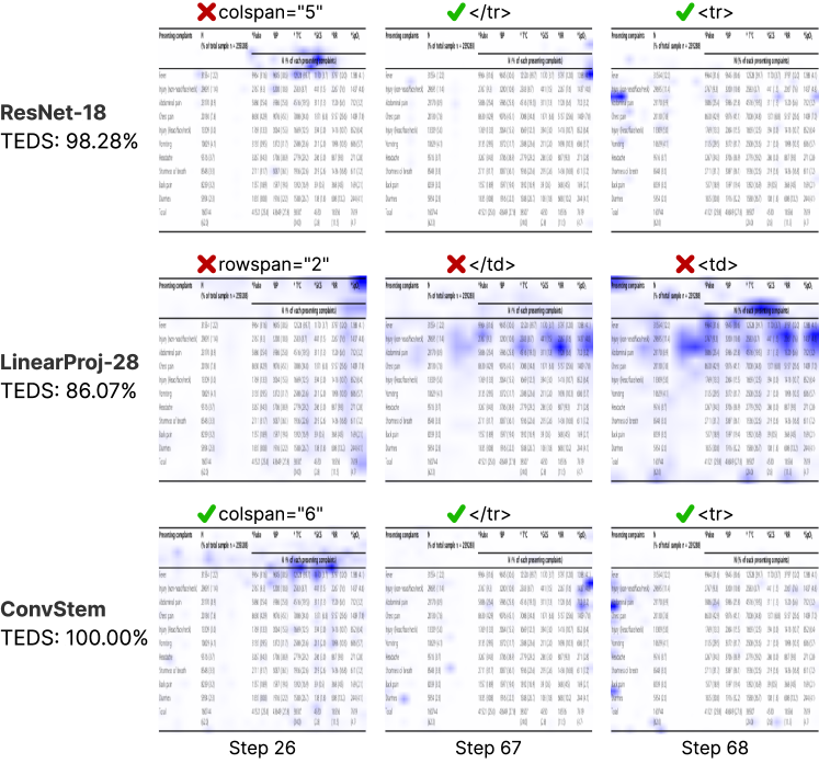
Figure 2: The convolutional stem accurately reconstructs the table; however, the CNN backbone miscounts columns in the header spanning cell. The linear projection’s scattered attention leads to the omission of predicting several complex table structures. The cross-attention maps (highlighted in blue) illustrate how the model processes various components of a table structure. We calculate the TEDS score for each model on this complex table. The HTML prediction is displayed above each individual attention map. The first column shows a header data cell that spans six columns, while the second and third columns visualize the beginning of a new data row.

4.3 Qualitative Analysis

In Fig. 2, we showcase the cross-attention maps of all three types of visual encoders, illustrating how the model processes various components of a table structure. In the first column of Fig. 2, we visualize a header data cell that spans six columns. Both ResNet-18 and ConvStem accurately focus on this spanning cell, but ResNet-18 miscalculates the number of columns it spans as the attention of ConvStem is more evenly scattered across six columns. For LinearProj-28, the attention erroneously centers on the top-right data cell and predicts a multi-row structure, i.e., rowspan=‘‘2’’. In the second and third columns of Fig. 2, we visualize the beginning of a new data row. For ResNet-18 and ConvStem, the attention concentrates on the end of the preceding row when predicting </tr> and successfully transitions to the start of the subsequent row when predicting the next token <tr>. However, LinearProj-28’s attention still focuses on the data cell due to the incorrect prediction in the early steps. In summary, the convolutional stem accurately reconstructs the table, whereas the CNN backbone makes an error in calculating the number of columns in a spanning cell. The attention of the linear projection is often dispersed, leading to the omission of predicting several complex table structures.

4.4 Ablations

This section investigates the root cause of the performance degradation from CNN backbone to linear projection and explains why convolutional stem can bridge this performance gap. We conduct a series of ablation experiments to delve deeper into the impacts of the receptive field and sequence length of the transformer. Sec. 4.4.1 introduces the concept of two factors that affect performance: RF ratio and sequence length $N$, and Sec. 4.4.2 analyzes these factors across different visual encoders, comparing their effects.

Table 2: The convolutional stem balances the model complexity, RF ratio, and sequence length, while still achieving competitive performance. We show ablations of how RF ratio and sequence length $N$ impact the performance of different visual encoders. In general, higher RF ratio and longer $N$ benefit TSR, especially with complex tables. Among these visual encoders, the CNN backbone is performant with exhaustive RF but exhibits high model complexity. Linear projection is the simplest but suffers in terms of performance due to limited RF and sequence length. We highlight the best model for each type of visual encoder.

							TEDS (%)
Model	#Param.	MAC	#Conv.	Kernel	RF ratio (%)	$N$	Simple	Complex	All
ResNet-18	28.70M	42.22G	17	-	97.10	784	98.31	94.50	96.45
ResNet-34	38.80M	71.87G	33	-	100.00	784	98.44	95.00	96.76
ResNet-50	41.81M	79.60G	49	-	95.31	784	98.44	94.89	96.70
LinearProj-14	21.89M	24.03G	1	14	3.13	1024	91.15	83.11	87.22
LinearProj-16	21.86M	19.21G	1	16	3.57	784	91.69	83.25	87.56
LinearProj-28	22.67M	10.28G	1	28	6.25	256	94.12	86.62	90.45
LinearProj-56	26.28M	7.60G	1	56	12.50	64	95.61	88.57	92.17
LinearProj-112	40.73M	6.98G	1	112	25.00	16	94.49	86.55	90.61
ConvStem-R1	22.53M	20.69G	5	3	6.92	784	97.68	93.36	95.57
ConvStem-R2	24.11M	22.36G	5	5	12.82	784	98.30	93.89	96.14
ConvStem-R3	22.14M	18.67G	4	5	12.95	729	97.97	93.99	96.02
ConvStem	24.08M	22.36G	5	5	13.62	729	98.33	94.66	96.53
ConvStem-N1	22.39M	10.55G	5	3	12.30	256	96.99	91.53	94.32
ConvStem-N2	23.98M	17.67G	5	5	15.56	528	98.03	93.65	95.89
ConvStem	24.08M	22.36G	5	5	13.62	729	98.33	94.66	96.53
ConvStem-N3	24.18M	26.82G	5	5	12.10	900	98.27	94.65	96.50

4.4.1 RF Ratio & Sequence Length

The RF is a key parameter in understanding the degree to which input signals may impact output features, and mapping features at any part of the network to the region in the input that generates them [31]. We define RF ratio as the size of this input region divided by the size of the entire input image on one side. Notably, the RF is solely determined by the model’s architecture, whereas increasing the image size alone has been demonstrated to enhance accuracy [32]. Therefore, the RF ratio is defined to exclude the influence of image size.

The sequence length $N$ is another important factor influencing the performance of the transformer. Training with a longer context generally yields higher-quality models [15], but the bottlenecks lie in the computation cost and memory of the attention layer: doubling $N$ would quadruple the runtime and memory requirements [33]. In our TSR model, the transformer receives the flattened feature map from the visual encoder, so $N$ is quadratic to the size of the feature map. Thus, reducing the feature map size can significantly improve the training and inference speed.

4.4.2 Analysis of Three Visual Encoders

In Table 2, we explore variations in the number of convolutional layers, kernel size, and input image size for each type of visual encoder. Alongside these configurations, we list details on total parameters, MAC and TEDS score for each model.

CNN backbone. We test three CNN backbones: ResNet-18, ResNet-34, and ResNet-50. Sequence length $N$ remains consistent across all three ResNets as they all downsample the input by a factor of 16. Comparing ResNet-18 to ResNet-34, the TEDS increases along with the increase of the RF ratio, as expected. In contrast, when comparing ResNet-34 to ResNet-50, the TEDS of simple tables are similar, but ResNet-50 has a worse TEDS of complex tables, despite having 3.01M more parameters. This discrepancy is exactly due to the reduction in the RF ratio in ResNet-50.

Linear projection. The RF ratio and $N$ are inversely correlated in linear projection. An increase in the RF ratio means a larger patch size $P$, resulting in a shorter sequence length $N=HW/P^{2}$. We ablate on five different patch sizes, ranging from 14 to 112. With the increase of the patch size, we can clearly observe a boost in the TEDS score, especially for the complex table. LinearProj-56 achieves the peak performance, and we observe a sharp decline in TEDS score when the RF ratio continues to increase. As previously mentioned, the RF ratio and $N$ exhibit an inverse correlation, and a significantly low $N$ reduces cross-attention among different patches, which leads to a performance reduction Consequently, due to this correlation, the performance of linear projection is capped by a specific patch size.

Convolutional stem. In Table 2, we perform separate ablations on the convolutional stem by tuning the number of convolution layers, kernel size, and input image size. While keeping $N$ fixed at $27^{2}$ or $28^{2}$, we observe the consistent trend that the TEDS increases along with the RF ratio. When we constrain the RF ratio within a certain range, increasing the value of $N$ further enhances performance.

In general, a higher RF ratio and longer sequence length to transformers are beneficial for TSR, particularly when dealing with complex tables. As shown in Fig. 1, a small RF provides only minimal structural information, while a medium-sized RF offers sufficient context and distinguishable features. Among the three types of visual encoders, the CNN backbone is performant with exhaustive RF but exhibits high model complexity. Linear projection is the simplest but suffers in terms of performance due to limited RF and sequence length. In contrast, the convolutional stem balances the model complexity, RF ratio, and sequence length, while still achieving competitive performance. These results also demonstrate the benefits of injecting the inductive bias of early convolution, especially locality, into the learning ability of transformers.

5 Conclusion

In this work, we design a lightweight visual encoder for TSR without sacrificing expressive power. We discover that a convolutional stem can match classic CNN backbone performance, with a much simpler model. The convolutional stem strikes an optimal balance between two crucial factors for high-performance TSR: a higher RF ratio and a longer sequence length. This allows it to “see” an appropriate portion of the table and “store” the complex table structure within sufficient context length for the subsequent transformer. We conducted reproducible ablation studies and open-sourced our code to enhance transparency, inspire innovations, and facilitate fair comparisons in our domain as tables are a promising modality for representation learning.

References

- Zhong et al. [2020] Xu Zhong, Elaheh ShafieiBavani, and Antonio Jimeno Yepes. Image-based table recognition: data, model, and evaluation. In European conference on computer vision, pages 564–580. Springer, 2020.
- Nassar et al. [2022] Ahmed Nassar, Nikolaos Livathinos, Maksym Lysak, and Peter Staar. Tableformer: Table structure understanding with transformers. In Proceedings of the IEEE/CVF Conference on Computer Vision and Pattern Recognition, pages 4614–4623, 2022.
- Huang et al. [2023] Yongshuai Huang, Ning Lu, Dapeng Chen, Yibo Li, Zecheng Xie, Shenggao Zhu, Liangcai Gao, and Wei Peng. Improving table structure recognition with visual-alignment sequential coordinate modeling. In Proceedings of the IEEE/CVF Conference on Computer Vision and Pattern Recognition, pages 11134–11143, 2023.
- Li et al. [2019] Minghao Li, Lei Cui, Shaohan Huang, Furu Wei, Ming Zhou, and Zhoujun Li. Tablebank: A benchmark dataset for table detection and recognition. arXiv preprint arXiv:1903.01949, 2019.
- Ye et al. [2021] Jiaquan Ye, Xianbiao Qi, Yelin He, Yihao Chen, Dengyi Gu, Peng Gao, and Rong Xiao. Pingan-vcgroup’s solution for icdar 2021 competition on scientific literature parsing task b: table recognition to html. arXiv preprint arXiv:2105.01848, 2021.
- He et al. [2016] Kaiming He, Xiangyu Zhang, Shaoqing Ren, and Jian Sun. Deep residual learning for image recognition. In Proceedings of the IEEE conference on computer vision and pattern recognition, pages 770–778, 2016.
- Vaswani et al. [2017] Ashish Vaswani, Noam Shazeer, Niki Parmar, Jakob Uszkoreit, Llion Jones, Aidan N Gomez, Łukasz Kaiser, and Illia Polosukhin. Attention is all you need. Advances in neural information processing systems, 30, 2017.
- Lu et al. [2019] Jiasen Lu, Dhruv Batra, Devi Parikh, and Stefan Lee. Vilbert: Pretraining task-agnostic visiolinguistic representations for vision-and-language tasks. Advances in neural information processing systems, 32, 2019.
- Chen et al. [2020] Yen-Chun Chen, Linjie Li, Licheng Yu, Ahmed El Kholy, Faisal Ahmed, Zhe Gan, Yu Cheng, and Jingjing Liu. Uniter: Universal image-text representation learning. In European conference on computer vision, pages 104–120. Springer, 2020.
- Huang et al. [2020] Zhicheng Huang, Zhaoyang Zeng, Bei Liu, Dongmei Fu, and Jianlong Fu. Pixel-bert: Aligning image pixels with text by deep multi-modal transformers. arXiv preprint arXiv:2004.00849, 2020.
- Dosovitskiy et al. [2020] Alexey Dosovitskiy, Lucas Beyer, Alexander Kolesnikov, Dirk Weissenborn, Xiaohua Zhai, Thomas Unterthiner, Mostafa Dehghani, Matthias Minderer, Georg Heigold, Sylvain Gelly, et al. An image is worth 16x16 words: Transformers for image recognition at scale. arXiv preprint arXiv:2010.11929, 2020.
- Li et al. [2022] Junlong Li, Yiheng Xu, Tengchao Lv, Lei Cui, Cha Zhang, and Furu Wei. Dit: Self-supervised pre-training for document image transformer. In Proceedings of the 30th ACM International Conference on Multimedia, pages 3530–3539, 2022.
- Bao et al. [2021] Hangbo Bao, Li Dong, Songhao Piao, and Furu Wei. Beit: Bert pre-training of image transformers. arXiv preprint arXiv:2106.08254, 2021.
- Xiao et al. [2021] Tete Xiao, Mannat Singh, Eric Mintun, Trevor Darrell, Piotr Dollár, and Ross Girshick. Early convolutions help transformers see better. Advances in neural information processing systems, 34:30392–30400, 2021.
- Tay et al. [2020] Yi Tay, Mostafa Dehghani, Samira Abnar, Yikang Shen, Dara Bahri, Philip Pham, Jinfeng Rao, Liu Yang, Sebastian Ruder, and Donald Metzler. Long range arena: A benchmark for efficient transformers. arXiv preprint arXiv:2011.04006, 2020.
- Deng et al. [2019] Yuntian Deng, David Rosenberg, and Gideon Mann. Challenges in end-to-end neural scientific table recognition. In 2019 International Conference on Document Analysis and Recognition (ICDAR), pages 894–901. IEEE, 2019.
- Wang et al. [2018] Xiaolong Wang, Ross Girshick, Abhinav Gupta, and Kaiming He. Non-local neural networks. In Proceedings of the IEEE conference on computer vision and pattern recognition, pages 7794–7803, 2018.
- Ramachandran et al. [2019] Prajit Ramachandran, Niki Parmar, Ashish Vaswani, Irwan Bello, Anselm Levskaya, and Jon Shlens. Stand-alone self-attention in vision models. Advances in neural information processing systems, 32, 2019.
- Kim et al. [2021] Wonjae Kim, Bokyung Son, and Ildoo Kim. Vilt: Vision-and-language transformer without convolution or region supervision. In International Conference on Machine Learning, pages 5583–5594. PMLR, 2021.
- Singh et al. [2023] Naman D Singh, Francesco Croce, and Matthias Hein. Revisiting adversarial training for imagenet: Architectures, training and generalization across threat models. arXiv preprint arXiv:2303.01870, 2023.
- Peng et al. [2023] ShengYun Peng, Weilin Xu, Cory Cornelius, Matthew Hull, Kevin Li, Rahul Duggal, Mansi Phute, Jason Martin, and Duen Horng Chau. Robust principles: Architectural design principles for adversarially robust cnns. arXiv preprint arXiv:2308.16258, 2023.
- Lu et al. [2021] Ning Lu, Wenwen Yu, Xianbiao Qi, Yihao Chen, Ping Gong, Rong Xiao, and Xiang Bai. Master: Multi-aspect non-local network for scene text recognition. Pattern Recognition, 117:107980, 2021.
- Paszke et al. [2017] Adam Paszke, Sam Gross, Soumith Chintala, Gregory Chanan, Edward Yang, Zachary DeVito, Zeming Lin, Alban Desmaison, Luca Antiga, and Adam Lerer. Automatic differentiation in pytorch. In NIPS-W, 2017.
- Araujo et al. [2019] André Araujo, Wade Norris, and Jack Sim. Computing receptive fields of convolutional neural networks. Distill, 4(11):e21, 2019.
- Cordonnier et al. [2019] Jean-Baptiste Cordonnier, Andreas Loukas, and Martin Jaggi. On the relationship between self-attention and convolutional layers. arXiv preprint arXiv:1911.03584, 2019.
- Zheng et al. [2021] Xinyi Zheng, Douglas Burdick, Lucian Popa, Xu Zhong, and Nancy Xin Ru Wang. Global table extractor (gte): A framework for joint table identification and cell structure recognition using visual context. In Proceedings of the IEEE/CVF winter conference on applications of computer vision, pages 697–706, 2021.
- Loshchilov and Hutter [2017] Ilya Loshchilov and Frank Hutter. Decoupled weight decay regularization. arXiv preprint arXiv:1711.05101, 2017.
- Jimeno Yepes et al. [2021] Antonio Jimeno Yepes, Peter Zhong, and Douglas Burdick. Icdar 2021 competition on scientific literature parsing. In Document Analysis and Recognition–ICDAR 2021: 16th International Conference, Lausanne, Switzerland, September 5–10, 2021, Proceedings, Part IV 16, pages 605–617. Springer, 2021.
- Sovrasov [2018-2023] Vladislav Sovrasov. ptflops: a flops counting tool for neural networks in pytorch framework, 2018-2023. URL https://github.com/sovrasov/flops-counter.pytorch.
- Rezatofighi et al. [2019] Hamid Rezatofighi, Nathan Tsoi, JunYoung Gwak, Amir Sadeghian, Ian Reid, and Silvio Savarese. Generalized intersection over union: A metric and a loss for bounding box regression. In Proceedings of the IEEE/CVF conference on computer vision and pattern recognition, pages 658–666, 2019.
- Le and Borji [2017] Hung Le and Ali Borji. What are the receptive, effective receptive, and projective fields of neurons in convolutional neural networks? arXiv preprint arXiv:1705.07049, 2017.
- Liu et al. [2022] Zhuang Liu, Hanzi Mao, Chao-Yuan Wu, Christoph Feichtenhofer, Trevor Darrell, and Saining Xie. A convnet for the 2020s. In Proceedings of the IEEE/CVF conference on computer vision and pattern recognition, pages 11976–11986, 2022.
- Dao et al. [2022] Tri Dao, Dan Fu, Stefano Ermon, Atri Rudra, and Christopher Ré. Flashattention: Fast and memory-efficient exact attention with io-awareness. Advances in Neural Information Processing Systems, 35:16344–16359, 2022.