Uncertainty-Aware Bayes’ Rule and Its Applications

Abstract

Bayes’ rule has enabled innumerable powerful algorithms of statistical signal processing and statistical machine learning. However, when there exist model misspecifications in prior distributions and/or data distributions, the direct application of Bayes’ rule is questionable. Philosophically, the key is to balance the relative importance of prior and data distributions when calculating posterior distributions: if prior (resp. data) distributions are overly conservative, we should upweight the prior belief (resp. data evidence); if prior (resp. data) distributions are overly opportunistic, we should downweight the prior belief (resp. data evidence). This paper derives a generalized Bayes’ rule, called uncertainty-aware Bayes’ rule, to technically realize the above philosophy, i.e., to combat the model uncertainties in prior distributions and/or data distributions. Simulated and real-world experiments showcase the superiority of the presented uncertainty-aware Bayes’ rule over the conventional Bayes’ rule: In particular, the uncertainty-aware Kalman filter, the uncertainty-aware particle filter, and the uncertainty-aware interactive multiple model filter are suggested and validated.

I Introduction

I-A Background

Beyes’ rule (or Bayes’ theorem) has countless successful applications in statistical signal processing, statistical machine learning, and bioinformatics such as Kalman filter, particle filter, Bayesian hypothesis testing, naive Bayes classifier, Bayesian optimization, Bayesian bandits, and Bayesian networks. Consider a data-generating distribution $p_{\bm{\theta}_{0}}(\bm{y})$ parametrized by unknown $\bm{\theta}_{0}\in\Theta\subseteq\mathbb{R}^{d}$ where $\Theta$ is the parameter space. We aim to estimate the true value $\bm{\theta}_{0}$ using $n$ collected samples $\{\bm{y}_{1},\bm{y}_{2},\ldots,\bm{y}_{n}\}\subset\mathcal{Y}$ from $p_{\bm{\theta}_{0}}(\bm{y})$ where $\mathcal{Y}\subseteq\mathbb{R}^{m}$ is the support set of $p_{\bm{\theta}_{0}}(\bm{y})$. Bayes’ rule

$$p(\bm{\theta}|\bm{y})\propto p(\bm{\theta})\cdot p(\bm{y}|\bm{\theta}),~{}~{}~{}\forall\bm{y}\in\mathcal{Y},~{}\forall\bm{\theta}\in\Theta$$ (1)

suggests the law of calculating the posterior distribution $p(\bm{\theta}|\bm{y})$ after observing the sample $\bm{y}$ using the likelihood function $\bm{\theta}\mapsto p(\bm{y}|\bm{\theta})\coloneqq p_{\bm{\theta}}(\bm{y})$ and the prior distribution $p(\bm{\theta})$. Philosophically, the prior distribution $p(\bm{\theta})$ encodes our prior belief that $\bm{\theta}\in\Theta$ is the true value and the likelihood function $p(\bm{y}|\bm{\theta})$ indicates our $\bm{y}$-data evidence that $\bm{\theta}$ is the true value; therefore, the posterior distribution $p(\bm{\theta}|\bm{y})$ denotes our integrated posterior belief that $\bm{\theta}$ is the true value. For a quick review of Bayes’ rule, see, e.g., [1].

I-B Problem Statement and Literature Review

In using the conventional Bayes’ rule (1), the fundamental assumption is that the data distribution $\bm{y}\mapsto p(\bm{y}|\bm{\theta})$ for every $\bm{\theta}\in\Theta$ and the prior distribution $p(\bm{\theta})$ are accurate: that is, the true value $\bm{\theta}_{0}$ is indeed a realization of $p(\bm{\theta})$ and the data $\{\bm{y}_{1},\bm{y}_{2},\ldots,\bm{y}_{n}\}$ are indeed sampled from $p_{\bm{\theta}_{0}}(\bm{y})$. However, this assumption is highly untenable in practice, and as a result, the performance of algorithms relying on the conventional Bayes’ rule (1) significantly degrades: For illustrations and justifications from the general Bayesian statistics community, see, e.g., [2, 3, 4, 5, 6]; for those from the Bayesian statistical signal processing community, see, e.g., [7, 8, 9, 10].

Facing the model uncertainties before applying Bayes’ rule, one way is to improve the modeling accuracy and reduce such uncertainties, for example, by replacing Gaussian distributions with Student’s $t$ distributions when outliers present [5, Chap. 17], and the other is to withstand the model uncertainties with robust methods, for example, using noninformative priors [2], using robust data distributions [11, Chaps. 4 and 5], [12, 13], or modifying the Bayes’ rule itself (e.g., $\alpha$-posterior) [14, Sec. 6.8.5 and Sec. 8.], [15, 6]. While it is not always practically easy to improve the modeling accuracy (because additional information is required, e.g., the knowledge that Student’s $t$ distributions can model measurement outliers), robust methods are attractive to practitioners. According to [11, Sec. 15.2], the key to the robust design is to balance the relative importance between the prior distribution (i.e., prior belief) and the data distribution (i.e., likelihood function, data evidence). To clarify further, if the prior distribution is uncertain (i.e., unreliable), we reduce the contribution of the prior distribution to the posterior distribution; likewise, if the data distribution is uncertain, we reduce the contribution of the data distribution to the posterior distribution. This idea has been empirically/theoretically validated and technically implemented in, e.g., [16], where the maximum entropy scheme is employed to diminish the importance of prior distributions or data distributions, and in, e.g., [14, Sec. 6.8.5 and Sec. 8.], where the $\alpha$-posterior scheme is employed to manage the importance of the data distributions using an $\alpha$-power operator (the importance of the data distributions is reduced if $0<\alpha<1$ and remains unchanged if $\alpha=1$).

However, the maximum entropy scheme is computationally complex: we prefer a computationally simpler scheme that has almost the same computational burden as the conventional Bayes’ rule and the $\alpha$-posterior scheme. To clarify further, we prefer a Bayes-rule-like formula that can function as the maximum entropy scheme. In addition, both the maximum entropy scheme and the $\alpha$-posterior scheme cannot technically augment the importance of prior distributions and data distributions: they can only diminish the importance of prior distributions and/or data distributions because as robust (i.e., conservative) methods, they tend to downweight the information (from prior belief or data evidence) at hands. Nevertheless, when the prior belief (resp. data evidence) is obtained in a conservative manner, it is beneficial if we can upweight the information from the prior belief (resp. data evidence).

In summary, a generalized Bayes’ rule that can balance the relative importance between prior belief and data evidence is expected. Furthermore, the new Bayes’ rule can not only downweight prior brief and data evidence but also upweight them when required, in a computationally efficient manner.

I-C Contributions

This paper mathematically formalizes and generalizes the philosophy in [11, Sec. 15.2], and an uncertainty-aware Bayes’ rule is derived. The generalization roots in moving to an uncertainty-aware design from the robust design in [11, Sec. 15.2]. Uncertainty awareness is more general than robustness because when the information (i.e., prior belief or data evidence) is believed to be opportunistic, we need to pursue robustness and downweight the information. In contrast, when the information is believed to be conservative, we need to abandon robustness and upweight the information.

The contributions of this paper can be itemized as follows.

1. We propose a new interpretation method of the conventional Bayes’ rule (1); see Lemma 1.

2. We propose an uncertainty-aware Bayes’ rule $p_{g}(\bm{\theta}|\bm{y})\propto p^{\beta}(\bm{\theta})\cdot p^{\alpha}(\bm{y}|\bm{\theta})$, called $(\alpha,\beta)$-posterior, where $\alpha,\beta\in[-\infty,\infty]$, that generalizes the conventional Bayes’ rule (1); see Theorem 1 and Definition 2.

3. We show that for some values of $\alpha$ and $\beta$, the uncertainty-aware Bayes’ rule can technically reflect the robustness (i.e., conservatism) philosophy in [11, Sec. 15.2], that is, to function as the maximum entropy scheme and the $\alpha$-posterior scheme (i.e., downweighting the prior belief and/or data evidence). For other values, the uncertainty-aware Bayes’ rule can reflect the opportunism philosophy and upweight the prior belief and/or data evidence. For details, see Theorems 2 and 3, and Insights 1 and 2.

4. We validate the superiority of the uncertainty-awareness design over the robustness design using both simulated and real-world experiments. For details, see Section III.

I-D Notations

Random and deterministic quantities are denoted by upright and Italic symbols (e.g., $\mathbf{y}$ and $\bm{y}$), respectively. Let $\mathbb{R}^{d}$ denote the $d$-dimensional real space. We use $p_{\mathbf{y}}(\bm{y})$ to denote the probability density (resp. mass) function of $\mathbf{y}$ if $\mathbf{y}$ is continuous (resp. discrete); when it is clear from the contexts, $p(\bm{y})$ is used as a shorthand for $p_{\mathbf{y}}(\bm{y})$. Let $\operatorname*{{Ent}}p(\bm{y})$ denote the (Shannon) entropy of the distribution $p(\bm{y})$: i.e., $\operatorname*{{Ent}}p(\bm{y})\coloneqq\int p(\bm{y})\cdot-\ln{p(\bm{y})}\mathrm{d}\bm{y}$. Let $\operatorname{KL}\left[{q(\bm{\theta})}\left\|{p(\bm{\theta})}\right.\right]$ define the Kullback–Leibler divergence of $q(\bm{\theta})$ from $p(\bm{\theta})$. The Gaussian distribution with mean $\bm{\mu}$ and covariance $\bm{\Sigma}$ is denoted as $\mathcal{N}(\bm{\mu},\bm{\Sigma})$ and its density function as $\mathcal{N}(\cdot;\bm{\mu},\bm{\Sigma})$. The running index set induced by integer $r$ is denoted as $[r]\coloneqq\{1,2,\ldots,r\}$.

II Main Results

This paper limits the presentation to the elementary probability theory and avoids using measure-theoretic languages. In addition, throughout the paper, we assume that the density function $p(\bm{y})$ exists and $0\leq p(\bm{y})<\infty$ for every $\bm{y}\in\mathcal{Y}$. To reduce the presentation length, main results are only given under probability density functions; for probability mass functions, one may just change integrals to sums. (Simplified proofs for discrete cases are possible since $p(\bm{y})\leq 1$ for every $\bm{y}$.) To reduce notational clutter, we implicitly mean $\bm{y}\in\mathcal{Y}$ and $\bm{\theta}\in\Theta$ throughout the paper, unless otherwise stated.

II-A Generalized Bayes’ Rule

We begin with the notion of likelihood distribution.

Definition 1 (Likelihood Distribution)

Let

$$l_{\bm{y}}(\bm{\theta})\coloneqq\frac{p(\bm{y}|\bm{\theta})}{\int p(\bm{y}|\bm{\theta})\mathrm{d}\bm{\theta}},~{}~{}~{}\forall\bm{y}$$ (2)

denote the likelihood distribution of $\bm{\theta}$ induced by the likelihood function $\bm{\theta}\mapsto p(\bm{y}|\bm{\theta})$ evaluated at the sample $\bm{y}$. When it is clear from the contexts, we suppress the notational dependence on $\bm{y}$ and use $l(\bm{\theta})$ as a shorthand for $l_{\bm{y}}(\bm{\theta})$. $\square$

The likelihood distribution $l(\bm{\theta})$ is a $\bm{y}$-parametric distribution of $\bm{\theta}$. A direct result of Definition 1 is that the posterior distribution $p(\bm{\theta}|\bm{y})$ given by the conventional Bayes’ rule (1) can also be expressed as

$$p(\bm{\theta}|\bm{y})\propto p(\bm{\theta})\cdot l(\bm{\theta}).$$ (3)

The lemma below gives an interpretation of the origin of the Bayes’ rule (3).

Lemma 1 (Conventional Bayes’ Rule)

The posterior distribution $p(\bm{\theta}|\bm{y})$ given by the Bayes’ rule (1) [or (3)] solves

$$\min_{q(\bm{\theta})}\operatorname{KL}\left[{q(\bm{\theta})}\left\|{p(\bm{\theta})}\right.\right]+\operatorname{KL}\left[{q(\bm{\theta})}\left\|{l(\bm{\theta})}\right.\right]+\operatorname*{{Ent}}q(\bm{\theta}).$$ (4)

Proof:

See Appendix A. $\square$∎

Lemma 1 suggests that the posterior distribution $p(\bm{\theta}|\bm{y})$ is an entropy-regularized $(\frac{1}{2},\frac{1}{2})$-KL-barycenter of the prior distribution $p(\bm{\theta})$ and the likelihood distribution $l(\bm{\theta})$; intuitively, $p(\bm{\theta}|\bm{y})$ is a minimum-entropy distribution that is simultaneously close to both the prior distribution (i.e., prior belief) and the likelihood distribution (i.e., $\bm{y}$-data evidence).

We generalize the optimization problem (4) to

$$\min_{q(\bm{\theta})}\alpha_{1}\operatorname{KL}\left[{q(\bm{\theta})}\left\|{p(\bm{\theta})}\right.\right]+\alpha_{2}\operatorname{KL}\left[{q(\bm{\theta})}\left\|{l(\bm{\theta})}\right.\right]+\alpha_{3}\operatorname*{{Ent}}q(\bm{\theta}),$$ (5)

where $0\leq\alpha_{1},\alpha_{2},\alpha_{3}\leq 1$ are weights; $\alpha_{1}+\alpha_{2}+\alpha_{3}=1$. We term the distribution solving the generalized problem (5) the generalized Bayes’ posterior distribution.

Theorem 1 (Generalized Bayes’ Rule)

The generalized posterior distribution $p_{g}(\bm{\theta}|\bm{y})$ solving (5) is given by

$$p_{g}(\bm{\theta}|\bm{y})\propto p^{\frac{\alpha_{1}}{1-2\alpha_{3}}}(\bm{\theta})\cdot l^{\frac{\alpha_{2}}{1-2\alpha_{3}}}(\bm{\theta}),$$ (6)

or equivalently,

$$p_{g}(\bm{\theta}|\bm{y})\propto p^{\frac{\alpha_{1}}{1-2\alpha_{3}}}(\bm{\theta})\cdot p^{\frac{\alpha_{2}}{1-2\alpha_{3}}}(\bm{y}|\bm{\theta}),$$ (7)

if $\alpha_{3}\neq 1/2$, provided that the right-hand-side terms are integrable on $\Theta$. When $\alpha_{3}=1/2$, $p_{g}(\bm{\theta}|\bm{y})$ is an arbitrary distribution supported on the set $\Theta^{*}$ where

$$\Theta^{*}\coloneqq\operatorname*{argmax}_{\bm{\theta}}\alpha_{1}\ln p(\bm{\theta})+\alpha_{2}\ln l(\bm{\theta})$$ (8)

contains all weighted maximum a-posteriori estimates.

Proof:

See Appendix B. $\square$∎

Eq. (8) can be understood as an $(\alpha_{1},\alpha_{2})$-weighted maximum posterior estimation. Motivated by the generalized posterior distribution in (6), we give the definition of the $(\alpha,\beta)$-posterior.

Definition 2 ($(\alpha,\beta)$-Posterior)

The $(\alpha,\beta)$-posterior induced by the prior distribution $p(\bm{\theta})$ and the likelihood distribution $l(\bm{\theta})$ is defined as

$$p_{g}(\bm{\theta}|\bm{y})\propto p^{\beta}(\bm{\theta})\cdot l^{\alpha}(\bm{\theta}),$$ (9)

where $-\infty<\alpha,\beta<\infty$, provided that the right-hand-side term is integrable on $\Theta$. When $\alpha=\beta=-\infty$ or $\alpha=\beta=\infty$, the $(\alpha,\beta)$-posterior $p_{g}(\bm{\theta}|\bm{y})$ is defined as an arbitrary distribution supported on $\Theta^{*}$ where $\Theta^{*}\coloneqq\operatorname*{argmax}_{\bm{\theta}}\alpha_{1}\ln p(\bm{\theta})+\alpha_{2}\ln l(\bm{\theta})$, for specified weights $0\leq\alpha_{1},\alpha_{2}\leq 1$ such that $\alpha_{1}+\alpha_{2}=1/2$. $\square$

The parameters $(\alpha,\beta)$ in $(\alpha,\beta)$-posterior can be negative. This is because, compared with (6), $\beta\coloneqq\frac{\alpha_{1}}{1-2\alpha_{3}}\in(-\infty,\infty)$ and $\alpha\coloneqq\frac{\alpha_{2}}{1-2\alpha_{3}}\in(-\infty,\infty)$. In addition, $\alpha$ and $\beta$ simultaneously tend to $-\infty$ (when $\alpha_{3}\downarrow 1/2$) or $\infty$ (when $\alpha_{3}\uparrow 1/2$); they have the same sign.

Below we give several motivational examples of the generalized Bayes’ rule (6) or (9); the first two of them are well-established and widely discussed in existing literature of Bayesian statistics.

Example 1 (Conventional Bayes’ Posterior)

The conventional Bayes’ rule (1) [resp. (3)] is a special case of the generalized Bayes’ rule (7) [resp. (6) or (9)] when $\alpha_{1}=\alpha_{2}=\alpha_{3}=1/3$ or $\alpha=\beta=1$. $\square$

Example 2 ($\alpha$-Posterior)

When $\alpha_{2}=\alpha_{3}\neq 1/2$, (6) reduces to

$$p_{g}(\bm{\theta}|\bm{y})\propto p(\bm{\theta})\cdot l^{\frac{\alpha_{2}}{\alpha_{1}}}(\bm{\theta}).$$ (10)

By letting $\alpha\coloneqq\frac{\alpha_{2}}{\alpha_{1}}$, we obtain the $\alpha$-posterior

$$p_{g}(\bm{\theta}|\bm{y})\propto p(\bm{\theta})\cdot l^{\alpha}(\bm{\theta}),$$ (11)

where $0\leq\alpha<\infty$. When $\alpha_{3}=1/2$, $p_{g}(\bm{\theta}|\bm{y})$ is an arbitrary distribution supported on $\Theta^{*}$ where $\Theta^{*}\coloneqq\operatorname*{argmax}_{\bm{\theta}}\ln l(\bm{\theta})$ contains all maximum likelihood estimates. $\square$

Note that in the $\alpha$-posterior, $\alpha\geq 0$. The $\alpha$-posterior in (11) is a well-established proposal in Bayesian statistics; see, e.g., [14, Sec. 6.8.5 and Sec. 8.6], [6, 15]. Given $0<\alpha<1$ and several other technical regularity conditions (e.g., $\Theta^{*}$ is a singleton), $\alpha$-posteriors can be shown to have posterior consistency (see [14, Thm. 6.54, Ex. 8.44] and [15]), asymptotic normality (see [6, Thm. 1]), and robustness against likelihood-model misspecifications (see [6, Sec. 4]); however, these conditions might be practically restrictive.

Example 3 ($\beta$-Posterior)

When $\alpha_{1}=\alpha_{3}\neq 1/2$, (6) reduces to

$$p_{g}(\bm{\theta}|\bm{y})\propto p^{\frac{\alpha_{1}}{\alpha_{2}}}(\bm{\theta})\cdot l(\bm{\theta}).$$ (12)

By letting $\beta\coloneqq\frac{\alpha_{1}}{\alpha_{2}}$, we obtain the $\beta$-posterior

$$p_{g}(\bm{\theta}|\bm{y})\propto p^{\beta}(\bm{\theta})\cdot l(\bm{\theta}),$$ (13)

where $0\leq\beta<\infty$. When $\alpha_{3}=1/2$, $p_{g}(\bm{\theta}|\bm{y})$ is an arbitrary distribution supported on $\Theta^{*}$ where $\Theta^{*}\coloneqq\operatorname*{argmax}_{\bm{\theta}}\ln p(\bm{\theta})$ contains all maximum prior estimates. $\square$

Note that in the $\beta$-posterior, $\beta\geq 0$. Compared with the $\alpha$-posterior in Example 2 that modifies the likelihood distribution $l(\bm{\theta})$, the $\beta$-posterior modifies the prior distribution $p(\bm{\theta})$.

Example 4 ($\gamma$-Posterior)

When $\alpha_{1}=\alpha_{2}$ and $\alpha_{3}\neq 1/2$, (6) reduces to

$$p_{g}(\bm{\theta}|\bm{y})\propto p^{\frac{\alpha_{1}}{4\alpha_{1}-1}}(\bm{\theta})\cdot l^{\frac{\alpha_{1}}{4\alpha_{1}-1}}(\bm{\theta}),$$ (14)

By letting $\gamma\coloneqq\frac{\alpha_{1}}{4\alpha_{1}-1}$, we obtain the $\gamma$-posterior

$$p_{g}(\bm{\theta}|\bm{y})\propto p^{\gamma}(\bm{\theta})\cdot l^{\gamma}(\bm{\theta}),$$ (15)

where $-\infty<\gamma<\infty$. When $\alpha_{3}=1/2$, $p_{g}(\bm{\theta}|\bm{y})$ is an arbitrary distribution supported on $\Theta^{*}$ where $\Theta^{*}\coloneqq\operatorname*{argmax}_{\bm{\theta}}\ln p(\bm{\theta})+\ln l(\bm{\theta})$ contains all usual maximum a-posteriori estimates. $\square$

Example 4 suggests an unusual fusion rule of the prior distribution $p(\bm{\theta})$ and the likelihood distribution $l(\bm{\theta})$; for example, when $\gamma=-1$ (i.e., $\alpha_{1}=1/5$), we have

$$p_{g}(\bm{\theta}|\bm{y})\propto\frac{1}{p(\bm{\theta})\cdot l(\bm{\theta})}.$$

Compared with the $\alpha$-posterior and the $\beta$-posterior, the $\gamma$-posterior modifies both the prior distribution and the likelihood distribution. In addition, $\gamma$ is allowed to be negative.

Example 5 ($\alpha$-Likelihood)

When $\alpha_{1}=0$ and $\alpha_{3}\neq 1/2$, (6) reduces to

$$p_{g}(\bm{\theta}|\bm{y})\propto l^{\frac{\alpha_{2}}{2\alpha_{2}-1}}(\bm{\theta}).$$ (16)

By letting $\alpha\coloneqq\frac{\alpha_{2}}{2\alpha_{2}-1}$, we obtain the $\alpha$-likelihood

$$p_{g}(\bm{\theta}|\bm{y})\propto l^{\alpha}(\bm{\theta}),$$ (17)

where $\alpha\in(-\infty,\infty)$. When $\alpha_{3}=1/2$, $p_{g}(\bm{\theta}|\bm{y})$ is an arbitrary distribution supported on $\Theta^{*}$ where $\Theta^{*}\coloneqq\operatorname*{argmax}_{\bm{\theta}}\ln l(\bm{\theta})$ contains all maximum likelihood estimates. $\square$

In the generalized Bayes’ posterior (17) induced by the $\alpha$-likelihood $l^{\alpha}(\bm{\theta})$, the prior distribution $p(\bm{\theta})$ is completely ignored. To clarify further, we only trust the likelihood distribution with the confidence level $\alpha$ and absolutely distrust the prior distribution.

Example 6 ($\alpha$-Prior)

When $\alpha_{2}=0$ and $\alpha_{3}\neq 1/2$, (6) reduces to

$$p_{g}(\bm{\theta}|\bm{y})\propto p^{\frac{\alpha_{1}}{2\alpha_{1}-1}}(\bm{\theta}).$$ (18)

By letting $\alpha\coloneqq\frac{\alpha_{1}}{2\alpha_{1}-1}$, we obtain the $\alpha$-prior

$$p_{g}(\bm{\theta}|\bm{y})\propto p^{\alpha}(\bm{\theta}),$$ (19)

where $\alpha\in(-\infty,\infty)$. When $\alpha_{3}=1/2$, $p_{g}(\bm{\theta}|\bm{y})$ is an arbitrary distribution supported on $\Theta^{*}$ where $\Theta^{*}\in\operatorname*{argmax}_{\bm{\theta}}\ln p(\bm{\theta})$ contains all maximum prior estimates. $\square$

In the generalized Bayes’ posterior (19) induced by the $\alpha$-prior $p^{\alpha}(\bm{\theta})$, the likelihood distribution $l(\bm{\theta})$ is completely ignored. To clarify further, we only trust the prior distribution with the confidence level $\alpha$ and absolutely distrust the likelihood distribution.

Example 7 ($\alpha$-Pooled Posterior)

When $\alpha_{3}=0$, (6) reduces to

$$p_{g}(\bm{\theta}|\bm{y})\propto p^{\alpha_{1}}(\bm{\theta})\cdot l^{\alpha_{2}}(\bm{\theta}).$$ (20)

By letting $\alpha_{1}\coloneqq\alpha$ and $\alpha_{2}\coloneqq 1-\alpha$, we obtain the $\alpha$-pooled-posterior

$$p_{g}(\bm{\theta}|\bm{y})\propto p^{\alpha}(\bm{\theta})\cdot l^{1-\alpha}(\bm{\theta}),$$ (21)

where $0\leq\alpha\leq 1$. $\square$

The $\alpha$-pooled-posterior in (21) is a $\alpha$-log-linear pooling [17, 18] of the prior distribution $p(\bm{\theta})$ and the likelihood distribution $l(\bm{\theta})$, which is an alternative of the linear pooling rule ${\alpha}p(\bm{\theta})+{(1-\alpha)}l(\bm{\theta})$. The log-linear pooling rule is standard in Bayesian statistics for fusing multiple priors (from multiple experts) to obtain an integrated prior [17]. However, the $\alpha$-pooled-posterior in (21) claims that the likelihood distribution can also be used as a “prior” where the collected data $\bm{y}$ serve as an expert. (But this data-driven expert does not insist on his/her opinion due to randomness of $\bm{y}$; he/she is a flexible expert; instead, conventional non-data-driven experts are stubborn.) In addition, from (5), we can see that when $\alpha_{3}=0$, the entropy regularizer is removed. Therefore, it is natural to imagine that the $\alpha$-pooled posterior in (21) has larger entropy than the conventional Bayes’ posterior $p(\bm{\theta}|\bm{y})$.

From Examples 1-7, we can see that the $(\alpha,\beta)$-posterior, compared to the conventional Bayes’ posterior (when $\alpha=\beta=1$), defines general fusing rules of the prior distribution $p(\bm{\theta})$ and the likelihood distribution $l(\bm{\theta})$; we refer to the law of defining the $(\alpha,\beta)$-posterior as the generalized Bayes’ rule.

II-B Properties of Generalized Bayes’ Rule

The definition of the $(\alpha,\beta)$-posterior motivates us to study the properties of $\alpha$-scaled distributions.

Definition 3 ($\alpha$-Scaled Distribution)

The $\alpha$-scaled distribution $h^{(\alpha)}(\bm{y})$ induced by the distribution $h(\bm{y})$ is defined as

$$h^{(\alpha)}(\bm{y})=\frac{h^{\alpha}(\bm{y})}{\int h^{\alpha}(\bm{y})\mathrm{d}\bm{y}},$$ (22)

for $-\infty<\alpha<\infty$, if $\int h^{\alpha}(\bm{y})\mathrm{d}\bm{y}$ exists. $\square$

As the definition implies, $h^{(\alpha)}(\bm{y})\equiv h(\bm{y})$ for every $\alpha$ if $h(\bm{y})$ is a uniform distribution on a finite support set $\mathcal{Y}$.

Theorem 2

Suppose that $h(\bm{y})$ is not a uniform distribution. The function $\alpha\mapsto\operatorname*{{Ent}}h^{(\alpha)}(\bm{y})$ is monotonically increasing in $\alpha$ on $(-\infty,0)$ and monotonically decreasing in $\alpha$ on $(0,\infty)$.

Proof:

See Appendix C. $\square$∎

In the following, we study the relation between the entropy of $h^{(\alpha)}(\bm{y})$ and the entropy of $h(\bm{y})$. Let $E(\alpha)$ denote the entropy difference evaluated at $\alpha\in(-\infty,\infty)$:

$$E(\alpha)\coloneqq\operatorname*{{Ent}}h^{(\alpha)}(\bm{y})-\operatorname*{{Ent}}h(\bm{y}).$$ (23)

Theorem 2 implies that $E(\alpha)$ is monotonically increasing when $-\infty<\alpha<0$ and monotonically decreasing otherwise. In addition, it is obvious to see that $E(0)>0$ and $E(1)=0$. As a result, the following corollary is immediate.

Corollary 1

If $0\leq\alpha<1$, then $h^{(\alpha)}(\bm{y})$ has larger entropy than $h(\bm{y})$; if $1<\alpha<\infty$, then $h^{(\alpha)}(\bm{y})$ has smaller entropy than $h(\bm{y})$. $\square$

A visual illustration of the entropy difference $E(\alpha)$ when $h(\bm{y})$ is discrete is given in Fig. 1; note that if $h(\bm{y})$ is a discrete distribution supported on finite atoms, $\alpha$ can be negative.

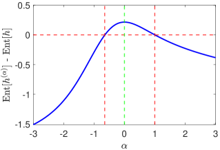
Figure 1: The entropy difference $E(\alpha)\coloneqq\operatorname*{{Ent}}h^{(\alpha)}(\bm{y})-\operatorname*{{Ent}}h(\bm{y})$ against $\alpha$; $h(\bm{y})$ is a randomly generated $10$-atom discrete distribution.

When $h(\bm{y})$ is continuous, a concrete example for Corollary 1 is as follows.

Example 8

Consider an one-dimensional zero-mean Gaussian density function $h(y)\propto e^{-\frac{1}{2}\frac{y^{2}}{\sigma^{2}}}$ where $\sigma^{2}$ is the variance. If $\alpha>0$, the $\alpha$-scaled distribution is $h^{(\alpha)}(y)\propto e^{-\frac{1}{2}\frac{y^{2}}{\sigma^{2}/\alpha}}$. Therefore, $h^{(\alpha)}(y)$ is a Gaussian density function with variance $\sigma^{2}/\alpha$. When $0<\alpha<1$, we have $\sigma^{2}/\alpha>\sigma^{2}$ and therefore $\operatorname*{{Ent}}h^{(\alpha)}(y)>\operatorname*{{Ent}}h(y)$; when $\alpha>1$, we have $\sigma^{2}/\alpha<\sigma^{2}$ and therefore $\operatorname*{{Ent}}h^{(\alpha)}(y)<\operatorname*{{Ent}}h(y)$. Note that $\operatorname*{{Ent}}h^{(\alpha)}(y)=\frac{1}{2}\ln(2\pi\sigma^{2}/\alpha)+\frac{1}{2}$, while $\operatorname*{{Ent}}h(y)=\frac{1}{2}\ln(2\pi\sigma^{2})+\frac{1}{2}$. $\square$

Theorem 2 and Corollary 1 collectively imply the following useful insight.

Insight 1 (Uncertainty Awareness in Posterior)

The $\alpha$-scaling operation controls the entropy (i.e., the uncertainty or our trust level) of $h^{(\alpha)}(\bm{y})$. Therefore, the $(\alpha,\beta)$-posterior $p_{g}(\bm{\theta}|\bm{y})\propto p^{\beta}(\bm{\theta})\cdot l^{\alpha}(\bm{\theta})$ balances the relative importance between the prior distribution $p(\bm{\theta})$ and the likelihood distribution $l(\bm{\theta})$. If we think that the likelihood (resp. prior) distribution is overly opportunistic, we use an $\alpha$ (resp. $\beta$) such that $\operatorname*{{Ent}}l^{(\alpha)}(\bm{\theta})$ [resp. $\operatorname*{{Ent}}p^{(\beta)}(\bm{\theta})$] is improved compared to $\operatorname*{{Ent}}l(\bm{\theta})$ [resp. $\operatorname*{{Ent}}p(\bm{\theta})$]; in contrast, if we think that the likelihood (resp. prior) distribution is overly conservative, we use an $\alpha$ (resp. $\beta$) such that $\operatorname*{{Ent}}l^{(\alpha)}(\bm{\theta})$ [resp. $\operatorname*{{Ent}}p^{(\beta)}(\bm{\theta})$] is reduced compared to $\operatorname*{{Ent}}l(\bm{\theta})$ [resp. $\operatorname*{{Ent}}p(\bm{\theta})$]. In addition, from the perspective of adjusting the trust level (i.e., the entropy) of a distribution, it suffices to consider only $\alpha\geq 0$ in practice. Therefore, if we do not trust much about the likelihood distribution (resp. the prior distribution), we use $0\leq\alpha<1$ (resp. $0\leq\beta<1$) if it is overly opportunistic, and use $\alpha>1$ (resp. $\beta>1$) if it is overly conservative. $\square$

Another reason to consider only $\alpha\geq 0$ in practice is due to the existence of the normalization factor $\int h^{\alpha}(\bm{y})\mathrm{d}\bm{y}$ in Definition 3. To be specific, for example, even for the popular Gaussian distributions, when $\alpha\leq 0$, the integral $\int h^{\alpha}(\bm{y})\mathrm{d}\bm{y}$ does not exist. However, in practice, $\alpha<0$ can provide additional flexibility in reshaping $h(\bm{y})$, beyond just adjusting its entropy (i.e., concentration); see, e.g., Fig. 3 later.

Next, we study the closeness to $h(\bm{y})$ from $h^{(\alpha)}(\bm{y})$.

Theorem 3

The closeness to $h(\bm{y})$ from $h^{(\alpha)}(\bm{y})$, i.e.,

$$\operatorname{KL}\left[{h(\bm{y})}\left\|{h^{(\alpha)}(\bm{y})}\right.\right],$$

is a monotonically increasing function if $1<\alpha<\infty$ and a monotonically decreasing function if $-\infty<\alpha<1$. In addition, it is a convex function in $\alpha$ on $(-\infty,\infty)$.

Proof:

See Appendix D. $\square$∎

A visual illustration of Theorem 3 when $h(\bm{y})$ is discrete is given in Fig. 2; note that in this case, $\alpha$ can be negative.

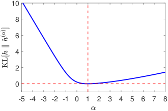
Figure 2: A visual illustration of the closeness $\operatorname{KL}\left[{h(\bm{y})}\left\|{h^{(\alpha)}(\bm{y})}\right.\right]$ to $h(\bm{y})$ from $h^{(\alpha)}(\bm{y})$; $h(\bm{y})$ is a randomly generated $10$-atom discrete distribution.

A concrete example for Theorem 3 when $h(\bm{y})$ is continuous is as follows.

Example 9

We continue studying the setup in Example 8. As a result, we have

$$\operatorname{KL}\left[{h(\bm{y})}\left\|{h^{(\alpha)}(\bm{y})}\right.\right]=-\frac{1}{2}\ln\left(\alpha\right)+\frac{\alpha}{2}-\frac{1}{2},~{}~{}~{}\alpha>0.$$

The derivative of $\operatorname{KL}\left[{h(\bm{y})}\left\|{h^{(\alpha)}(\bm{y})}\right.\right]$ with respect to $\alpha$ is $\frac{1}{2}(1-\frac{1}{\alpha})$, which is positive if $\alpha>1$ and negative if $0<\alpha<1$; the second-order derivative is $\frac{1}{2\alpha^{2}}>0$. Therefore, $\operatorname{KL}\left[{h(\bm{y})}\left\|{h^{(\alpha)}(\bm{y})}\right.\right]$ is monotonically decreasing when $0<\alpha<1$ and monotonically increasing when $\alpha>1$. In addition, $\operatorname{KL}\left[{h(\bm{y})}\left\|{h^{(\alpha)}(\bm{y})}\right.\right]$ is convex. $\square$

Theorem 3 implies the following useful insight.

Insight 2 (Level of Uncertainty)

The more $\alpha$ deviates from $1$, the farther to $h(\bm{y})$ from $h^{(\alpha)}(\bm{y})$. Therefore, in $(\alpha,\beta)$-posterior, the more we trust the prior distribution $p(\bm{\theta})$ [resp. the likelihood distribution $l(\bm{\theta})$], the closer the value of $\beta$ (resp. $\alpha$) should be to $1$. $\square$

Insights 1 and 2 collectively suggest the usage of the $(\alpha,\beta)$-posterior in practice.

II-C Outlier Treatment

With $0<\alpha<1$, the $\alpha$-scaled data distribution $p^{\alpha}(\bm{y}|\bm{\theta})$ has fatter tails than the unscaled data distribution $p(\bm{y}|\bm{\theta})$, and therefore, outliers in measurements can be accounted for. In addition to the $\alpha$-scaling operation, when outliers are present in measurements, outlier-unaware data distributions (e.g., Gaussian) can be modified to outlier-aware ones such as Student’s $t$ distributions, Laplace distributions, or $\varepsilon$-contamination and $\varepsilon$-normal distributions [12, p. 81 and p. 92], [19, Lems. 1 and 2]. In numerical operations when data distributions have no closed-form expressions, outlier treatment (including outlier rejection and outlier censoring) methods can be found in [16, Subsec. IV-C], [10, p. 88].

II-D Generalized Bayes’ Rule for Multiple Samples

When we have more than one, but i.i.d., sample (e.g., $n$ i.i.d. samples $\{\bm{y}_{1},\bm{y}_{2},\ldots,\bm{y}_{n}\}$), we can straightforwardly generalize (5) to

$$\begin{array}[]{l}\displaystyle\min_{q(\bm{\theta})}\alpha_{3}\operatorname*{{Ent}}q(\bm{\theta})+\alpha_{1}\operatorname{KL}\left[{q(\bm{\theta})}\left\|{p(\bm{\theta})}\right.\right]+\\ \quad\quad\quad\quad\displaystyle\frac{\alpha_{2}}{n}\sum^{n}_{i=1}\operatorname{KL}\left[{q(\bm{\theta})}\left\|{l_{\bm{y}_{i}}(\bm{\theta})}\right.\right].\end{array}$$ (24)

The solution of (24) is given in the corollary below.

Corollary 2 (Multi-sample Generalized Bayes’ Rule)

The generalized Bayes’ posterior solving (24) for $n$ i.i.d. samples is given by

$$p_{g}(\bm{\theta}|\bm{y}_{1},\ldots,\bm{y}_{n})\propto p^{\frac{\alpha_{1}}{1-2\alpha_{3}}}(\bm{\theta})\cdot\left[\prod^{n}_{i=1}l^{\frac{1}{n}}_{\bm{y}_{i}}(\bm{\theta})\right]^{\frac{\alpha_{2}}{1-2\alpha_{3}}},$$ (25)

if $\alpha_{3}\neq 1/2$, provided that the right-hand-side term is integrable on $\Theta$. When $\alpha_{3}=1/2$, $p_{g}(\bm{\theta}|\bm{y}_{1},\ldots,\bm{y}_{n})$ is an arbitrary distribution supported on the set $\Theta^{*}$ where

$$\Theta^{*}\coloneqq\operatorname*{argmax}_{\bm{\theta}}\alpha_{1}\ln p(\bm{\theta})+\alpha_{2}\cdot\frac{1}{n}\sum^{n}_{i=1}\ln l_{\bm{y}_{i}}(\bm{\theta})$$ (26)

is the weighted maximum posterior estimation; if further $\alpha_{1}=0$, (26) reduces to the maximum likelihood estimation. $\square$

The $(\alpha,\beta)$-posterior in Definition 2 under $n$ i.i.d. samples, induced by (25), can be rewritten as

$$p_{g}(\bm{\theta}|\bm{y}_{1},\ldots,\bm{y}_{n})\propto p^{\beta}(\bm{\theta})\cdot\prod^{n}_{i=1}l^{\frac{\alpha}{n}}_{\bm{y}_{i}}(\bm{\theta}),~{}~{}-\infty\leq\alpha,\beta\leq\infty.$$ (27)

Examples 1-7 can be restated accordingly; we do not repeat here.

As the data size increases (i.e., $n\uparrow\infty$), data-evidence becomes dominating and we can therefore let $\alpha_{1}$ depend on $n$ and $\alpha_{1,n}\to 0$ as $n\to\infty$. An example of $\alpha_{1,n}$ can be $\alpha_{1,n}\coloneqq 1/n$, or $1/n^{2}$ for a faster vanishing rate. As a result, $p_{g}(\bm{\theta}|\bm{y}_{1},\ldots,\bm{y}_{n})$ is asymptotically equal to an $\alpha$-scaled likelihood distribution; cf. Example 5.

II-E Examples of Application

The generalized (or uncertainty-aware) Bayes’ rule (9), i.e., the $(\alpha,\beta)$-posterior, has several potential applications in statistical signal processing and statistical machine learning.

First, we give an example of application in statistical signal processing.

Example 10 (Uncertainty-Aware Particle Filter)

Suppose that $\Theta$ is a finite discrete set containing $r$ points (each point is known as a particle): i.e., $\Theta\coloneqq\{\bm{\theta}_{1},\bm{\theta}_{2},\ldots,\bm{\theta}_{r}\}$. For each particle $\bm{\theta}_{i}$, $i\in[r]$, the likelihood evaluated at the measurement $\bm{y}$ is assumed to be $p(\bm{y}|\bm{\theta}_{i})$. Further, we suppose that the prior distribution is $\bm{p}\coloneqq[p_{1},p_{2},\ldots,p_{r}]$ and the $\bm{y}$-likelihood distribution (recall Definition 1) is $\bm{l}\coloneqq[l_{1},l_{2},\ldots,l_{r}]$. Then the generalized Bayes’ posterior, i.e., the $(\alpha,\beta)$-posterior, of particles is equal to

$$p_{g}(\bm{\theta}_{i}|\bm{y})\propto p^{\beta}_{i}\cdot l^{\alpha}_{i},~{}~{}~{}\forall i\in[r].$$

The above formula induces the uncertainty-aware particle filter for dynamic stochastic nonlinear systems. $\square$

Next, we give an example of application in statistical machine learning. It is shown that the uncertainty-aware Maximum A-Posteriori (MAP) estimation can lead to the popular ridge regression.

Example 11 (Uncertainty-Aware MAP Estimation)

We consider a nonlinear regression model $\mathrm{y}=f(\mathbf{x};\bm{\theta})+\mathrm{\epsilon}$ where $\mathrm{y}\in\mathbb{R}$ is the response, $\mathbf{x}\in\mathbb{R}^{m}$ is the feature vector, $\mathrm{\epsilon}\sim\mathcal{N}(0,1)$ is the regression error, and $\bm{\theta}$ is the parameter vector. Supposing the prior distribution of $\bm{\theta}$ is $\mathcal{N}(\bm{0},\bm{I}_{d})$, upon the collection of the data $(y,\bm{x})$, the MAP estimator of $\bm{\theta}$ is

$$\min_{\bm{\theta}\in\Theta}[y-f(\bm{x};\bm{\theta})]^{2}+\bm{\theta}^{\top}\bm{\theta}.$$

By using the $(\alpha,\beta)$-posterior rule, the uncertainty-aware MAP estimator of $\bm{\theta}$ can be written as

$$\min_{\bm{\theta}\in\Theta}{\alpha}[y-f(\bm{x};\bm{\theta})]^{2}+{\beta}\bm{\theta}^{\top}\bm{\theta}.$$

By letting $\lambda\coloneqq\beta/\alpha$, we have the $\lambda$-ridge regression

$$\min_{\bm{\theta}\in\Theta}[y-f(\bm{x};\bm{\theta})]^{2}+\lambda\bm{\theta}^{\top}\bm{\theta}.$$

Therefore, the popular ridge regression method in statistical machine learning can be interpreted as a consequence of uncertainty-aware MAP estimation. $\square$

II-F Illustration Examples

First, we visualize the $\alpha$-scaled distribution $h^{(\alpha)}(\bm{y})$ when $h(\bm{y})$ is discrete; see Fig. 3. From Fig. 3, we observe that the effect of a negative $\alpha$ is to reverse the relative importance of atoms. To clarify further, for example, suppose $\bm{h}\coloneqq[0.25,0.75]$. We have $\bm{h}^{(-1)}=[0.75,0.25]$; that is, the first atom, which has a smaller mass than the second before scaling, has a larger mass after scaling.

Figure 3: A $3$-atom discrete distribution $h(y)$ and induced $h^{(\alpha)}(y)$ with different $\alpha\in\{\pm 2,\pm 0.5\}$. Under $\alpha=\pm 0.5$, $\operatorname*{{Ent}}h^{(\alpha)}(y)>\operatorname*{{Ent}}h(y)$ (i.e., the former has more balanced masses, while the latter has more unbalanced masses). Under $\alpha=\pm 2$, $\operatorname*{{Ent}}h^{(\alpha)}(y)<\operatorname*{{Ent}}h(y)$. The effect of a negative $\alpha$ is to reverse the relative importance (i.e., probability mass) of atoms.

Next, we visualize the $(\alpha,\beta)$-posterior, compared with the conventional Bayes’ posterior. We focus on a mean estimation problem where $\theta_{0}$ is the true mean of the random variable $\mathrm{y}$. We suppose that the prior distribution is $p(\theta)\coloneqq\mathcal{N}(\theta;0,1)$. The likelihood function is $\theta\mapsto\mathcal{N}(y;\theta,1)$; if we assume that the measurement is $y\coloneqq 5$, the likelihood distribution is therefore $l(\theta)\coloneqq\mathcal{N}(\theta;5,1)$. The visualizations of the $(\alpha,\beta)$-posterior, under different value pairs of $(\alpha,\beta)$, are given in Fig. 4. As motivational examples, we only interpret the first three sub-figures. In Fig. 4(a), $\alpha=0$ means that the likelihood distribution is absolutely unreliable and the data evidence is completely ignored. Therefore, the $(0,2.5)$-posterior distribution tends to overlap with the prior distribution. Moreover, because $\beta=2.5>1$, the specified prior distribution is thought to be overly conservative and we propose to improve its concentration. In Fig. 4(b), $\alpha=\beta=0.5$ means that both the prior distribution and the posterior distribution are believed to be overly opportunistic, and therefore, we propose to reduce their concentration. As a result, the $(0.25,0.25)$-posterior distribution has larger entropy than the conventional Bayes’ posterior distribution. In Fig. 4(c), since $\alpha=0.25<0.5=\beta$, both the prior distribution and the likelihood distribution are thought to be opportunistic, but the prior distribution is thought to be less opportunistic than the likelihood distribution.

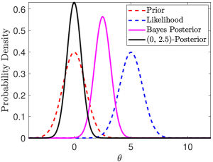
(a) $(0,2.5)$-posterior

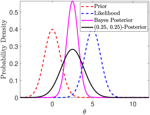
(b) $(0.25,0.25)$-posterior

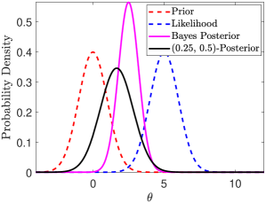
(c) $(0.25,0.5)$-posterior

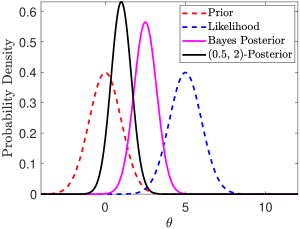
(d) $(0.5,2)$-posterior

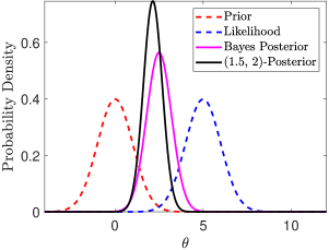
(e) $(1.5,2)$-posterior

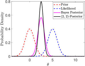
(f) $(2,2)$-posterior

Figure 4: Illustrative examples of $(\alpha,\beta)$-posterior. The prior distribution is $p(\theta)\coloneqq\mathcal{N}(\theta;0,1)$. The likelihood distribution is $l_{\bm{y}\coloneqq 5}(\theta)\coloneqq\mathcal{N}(\theta;5,1)$.

III Concrete Applications

The generalized (or uncertainty-aware) Bayes’ rule (9) can give birth to several Uncertainty-Aware Bayesian Signal Processing (UA-BSP) methods. As demonstrations and without loss of generality, in this section, we focus on state estimation (i.e., state filtering) problems of dynamic stochastic state-space systems. From the perspective of applied statistics, state estimation problems can be interpreted as sequential Bayesian inference. Briefly speaking, state estimation aims to estimate the unknown (i.e., unobservable) state vector $\mathbf{x}_{k}$ at the discrete time step $k$ using the known (i.e., observable) measurement set $\mathcal{Y}_{k}\coloneqq(\mathbf{y}_{1},\mathbf{y}_{2},\ldots,\mathbf{y}_{k})$ and the probabilistic model $p_{\mathbf{x}_{k},\mathcal{Y}_{k}}(\bm{x}_{k},\bm{Y}_{k})$; the probabilistic model $p_{\mathbf{x}_{k},\mathcal{Y}_{k}}(\bm{x}_{k},\bm{Y}_{k})$ is induced by the stochastic state-space models. The aim of state estimation is to obtain the posterior state distribution $p_{\mathbf{x}_{k}|\mathcal{Y}_{k}}(\bm{x}_{k}|\bm{Y}_{k})$ or the posterior mean $\mathbb{E}(\mathbf{x}_{k}|\mathcal{Y}_{k})$. All the source data and codes are available online at GitHub: https://github.com/Spratm-Asleaf/Bayes-Rule. The experimental results are obtained by a Lenovo laptop with 16G RAM and 11th Gen Intel(R) Core(TM) i5-11300H CPU @ 3.10GHz.

III-A Uncertainty-Aware Kalman Filter

We consider the state estimation problem of linear Gaussian state-space models [20, Chap. 3]

$$\left\{\begin{array}[]{rllll}\mathbf{x}_{k}&=\bm{F}_{k-1}\mathbf{x}_{k-1}+\bm{G}_{k-1}\mathbf{w}_{k-1},\\ \mathbf{y}_{k}&=\bm{H}_{k}\mathbf{x}_{k}+\mathbf{v}_{k},\end{array}\right.$$ (28)

where, for every time $k$, the system matrices $\bm{F}_{k}$, $\bm{G}_{k}$, and $\bm{H}_{k}$ are assumed to be known. The process noise vector and the measurement noise vector are denoted by $\mathbf{w}_{k}\sim\mathcal{N}(\bm{0},\bm{Q}_{k})$ and $\mathbf{v}_{k}\sim\mathcal{N}(\bm{0},\bm{R}_{k})$, respectively, and $\bm{Q}_{k}$ and $\bm{R}_{k}$ are assumed to be known, for every $k$. For this linear Gaussian system, under several uncorrelatedness assumptions among $\mathbf{x}_{0}$, $\{\mathbf{w}_{k}\}_{\forall k}$, and $\{\mathbf{v}_{k}\}_{\forall k}$ (see [20, p. 38]), the Kalman filter is the optimal state estimator in the sense of minimum mean-squared error.

Suppose that at time $k-1$, the posterior state distribution is

$$\hat{\mathbf{x}}_{k-1|k-1}\sim\mathcal{N}(\hat{\bm{x}}_{k-1|k-1},\bm{P}_{k-1|k-1}).$$

At time $k$, the prior state distribution is

$$\hat{\mathbf{x}}_{k|k-1}\sim\mathcal{N}(\hat{\bm{x}}_{k|k-1},\bm{P}_{k|k-1})$$

where $\bm{P}_{k|k-1}\coloneqq\bm{F}_{k-1}\bm{P}_{k-1|k-1}\bm{F}^{\top}_{k-1}+\bm{G}_{k-1}\bm{Q}_{k-1}\bm{G}^{\top}_{k-1}$ and $\hat{\bm{x}}_{k|k-1}\coloneqq\bm{F}_{k-1}\hat{\bm{x}}_{k-1|k-1}$; the measurement distribution conditioned on state $\mathbf{x}_{k}$ is

$$\mathbf{y}_{k}|\mathbf{x}_{k}\sim\mathcal{N}(\bm{H}_{k}\mathbf{x}_{k},\bm{R}_{k}).$$

Therefore, by applying the $(\alpha,\beta)$-posterior rule (9), the prior state distribution should be modified to

$$\hat{\mathbf{x}}_{k|k-1}\sim\mathcal{N}(\hat{\bm{x}}_{k|k-1},~{}\bm{P}_{k|k-1}/\beta)$$

and the conditional measurement distribution should be modified to

$$\mathbf{y}_{k}|\mathbf{x}_{k}\sim\mathcal{N}(\bm{H}_{k}\mathbf{x}_{k},~{}\bm{R}_{k}/\alpha).$$

Note that for a Gaussian distribution $\mathcal{N}(\bm{\mu},\bm{\Sigma})$, the $\alpha$-scaled version is equal to $\mathcal{N}(\bm{\mu},\bm{\Sigma}/\alpha)$. As a result, the $(\alpha,\beta)$-uncertainty-aware Kalman filter can be accordingly obtained by just applying the following two assignment operations in each Kalman iteration: $\bm{P}_{k|k-1}\leftarrow\bm{P}_{k|k-1}/\beta$ and $\bm{R}_{k}\leftarrow\bm{R}_{k}/\alpha$, for $\alpha,\beta>0$.

This modification rule is reminiscent of the distributionally robust state estimation (DRSE) method proposed in [21]; see also [10, p. 22, p. 53] for intuitive interpretations. Hence, when $0<\alpha,\beta\leq 1$, the $(\alpha,\beta)$-uncertainty-aware Kalman filter is equivalent to distributionally robust state estimation methods in [21, 19], provided that there are no outliers in measurements. Since $0<\alpha,\beta\leq 1$, $\bm{P}_{k|k-1}$ and $\bm{R}_{k}$ are assumed to be overly opportunistic, and therefore, they need to be inflated. When $\alpha,\beta\geq 1$, the values of $\bm{P}_{k|k-1}$ and $\bm{R}_{k}$ are reduced, which implies that $\bm{P}_{k|k-1}$ and $\bm{R}_{k}$ are assumed to be overly conservative. However, from the technical derivations of the DRSE method, the value reduction of $\bm{P}_{k|k-1}$ and $\bm{R}_{k}$ cannot be achieved in the DRSE method. In this sense, therefore, the $(\alpha,\beta)$-uncertainty-aware Kalman filter presented in this paper generalizes the DRSE method in [21, 19] when there are no measurement outliers: the former can handle not only opportunistic cases (by inflating covariances) but also conservative cases (by reducing covariances), while the latter can only address opportunistic cases. (NB: To combat opportunism is to introduce robustness/conservatism; i.e., robust methods innately cannot fight against conservatism.)

The experiments of the DRSE method in [10, Chap. 2] can sufficiently support the practical values of the $(\alpha,\beta)$-uncertainty-aware Kalman filter; just notice the mathematical equivalence to the DRSE method (when $0<\alpha,\beta\leq 1$). We do not repeat these experiments here.

III-B Uncertainty-Aware Particle Filter

The particle filter is standard to handle the state estimation problem of nonlinear systems [22]. By employing the $(\alpha,\beta)$-posterior in (9), the $(\alpha,\beta)$-uncertainty-aware particle filter can be straightforwardly obtained; see Example 10.

As an illustration, we specifically consider the state estimation problem of a one-dimensional nonlinear system model [23, 22, 16]

$$\left\{\begin{array}[]{cl}\mathrm{x}_{k}&=\displaystyle\frac{\mathrm{x}_{k-1}}{2}+\displaystyle\frac{25\mathrm{x}_{k-1}}{1+\mathrm{x}_{k-1}^{2}}+8\cos(1.2k)+\mathrm{w}_{k-1},\\ \mathrm{y}_{k}&=\displaystyle\frac{\mathrm{x}^{2}_{k}}{20}+0.5\sin(\mathrm{x}_{k})+\mathrm{v}_{k},\end{array}\right.$$ (29)

where for every $k$, $\mathrm{w}_{k}\sim\mathcal{N}(0,10)$ and $\mathrm{v}_{k}\sim\mathcal{N}(0,1)$; for every $k_{1}$ and $k_{2}$, $\mathrm{w}_{k_{1}}$ and $\mathrm{w}_{k_{2}}$ are uncorrelated, so are $\mathrm{v}_{k_{1}}$ and $\mathrm{v}_{k_{2}}$; for every $k$, $\mathrm{w}_{k}$ and $\mathrm{v}_{k}$ are uncorrelated. As in [16], we assume that the nominal measurement equation is

$$\mathrm{y}_{k}=\displaystyle\frac{\mathrm{x}^{2}_{k}}{20}+\mathrm{v}_{k},$$

which is slightly different from the true one in (29). Therefore, in this case, there is a modeling uncertainty in the measurement equation, i.e., in likelihood distributions at every $k$. As a result, to combat this model uncertainty and improve the filtering accuracy, we should use $\beta=1$ and $\alpha<1$.

For the purpose of experimental demonstration, we use $50$, $100$, and $200$ particles, respectively, to report the performance of the $(\alpha,1)$-uncertainty-aware particle filter. The systematic resampling method is adopted to address particle degeneracy, and the effective sample size is set to half the number of particles. Given the number of particles, the experiment is independently conducted with $500$ episodes and each episode contains $100$ time steps. The performance measure, in every episode, is the rooted time-averaged mean-squared error (RTAMSE) along $100$ time steps, i.e.,

$$\sqrt{\displaystyle\frac{1}{100}\sum_{k=1}^{100}(x_{k}-\hat{x}_{k})^{2}}$$

where $\hat{x}_{k}$ denotes the estimate of the true value $x_{k}$; the overall performance measure for a given number of particles is the averaged RTAMSEs of the $500$ episodes. The filtering result of the $(\alpha,1)$-uncertainty-aware particle filter is shown in Fig. 5, plotted against the value of $\alpha$.

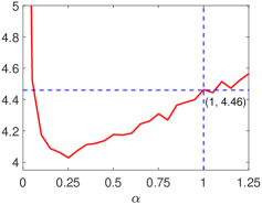
(a) 50 Particles

(b) 100 Particles

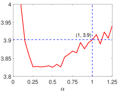
(c) 200 Particles

Figure 5: Averaged-RTAMSE performance of the $(\alpha,1)$-uncertainty-aware particle filter, against the value of $\alpha$. The larger the number of particles, the smaller the averaged RTAMSE. For a given number of particles, the $(\alpha,1)$-uncertainty-aware particle filter with $\alpha\approx 0.25$ works best.

As we can see from Fig. 5, when $\alpha<1$ but $\alpha$ is not close to zero, the $(\alpha,1)$-uncertainty-aware particle filter can outperform the conventional particle filter: This is because when there exists model uncertainty in the measurement equation, the likelihood distribution of particles at each time step tends to be unreliable, and therefore, we need to reduce the concentration (i.e., reduce the trust level and improve the entropy) of the likelihood distribution to cope with the uncertainty. In addition, the results suggest that the superiority of the $(\alpha,1)$-uncertainty-aware particle filter tends to be more significant as the number of particles decreases: This implies that the $(\alpha,1)$-uncertainty-aware particle filter has the innate ability to fight against the particle degeneracy issue. When $\alpha$ is overly small (i.e., close to zero), the $(\alpha,1)$-uncertainty-aware particle filter almost ignores information from the measurements, and therefore, the filter diverges: This indicates that uncertain information is at least better than no information.

III-C Uncertainty-Aware Interactive Multiple Model Filter

The interactive multiple model (IMM) filter is standard to handle the state estimation problem of jump linear systems [24, 25]. By employing the $(\alpha,\beta)$-posterior in (9), the $(\alpha,\beta)$-uncertainty-aware IMM filter can be straightforwardly obtained. One may just imagine the models’ prior weights as a prior distribution and the models’ likelihoods (evaluated at a given measurement) as a likelihood distribution; the aim is to infer the models’ posterior distribution and then compute the posterior state estimate.

As an illustration, we consider two real-world one-dimensional multi-model target tracking problems; as claimed in [26], focusing on only one coordinate does not lose the generality because the motions of a dynamic target in different coordinates can be independently tracked. Mathematically, it is a state estimation problem of a jump linear system model [27, 28, 29]

$$\left\{\begin{array}[]{l}\mathbf{x}_{k}=\left[\begin{array}[]{cc}1&T\\ 0&1\end{array}\right]\mathbf{x}_{k-1}+\left[\begin{array}[]{c}{T^{2}}/{2}\\ T\end{array}\right][\mathrm{a}_{\mathrm{j}_{k-1},k-1}+\mathrm{w}_{k-1}]\\ \mathrm{y}_{k}=\mathrm{p}_{k}+\mathrm{v}_{k},\end{array}\right.$$

where the state vector $\mathbf{x}_{k}$ is defined as $\mathbf{x}_{k}\coloneqq[\mathrm{p}_{k},\mathrm{s}_{k}]^{\top}$; $\mathrm{p}_{k}\in\mathbb{R}$ denotes the position, $\mathrm{s}_{k}\in\mathbb{R}$ the speed, and $\mathrm{a}_{\mathrm{j}_{k},k}\in\mathbb{R}$ the maneuvering acceleration of a moving target at time $k$; the positive-integer-valued discrete random variable $\mathrm{j}_{k}$ denotes the system’s operating mode at time $k$; $T>0$ is the sampling time between two discrete time indices; $\mathrm{w}_{k}\in\mathbb{R}$ is the acceleration modeling noise and $\mathrm{v}_{k}\in\mathbb{R}$ the sensor’s observation noise at time $k$. At time $k$, the maneuvering acceleration may randomly take any one of the following values

$$\mathrm{a}_{j_{k},k}=\left\{\begin{array}[]{ll}0,&j_{k}=1,\\ 10,&j_{k}=2,\\ -10,&j_{k}=3,\end{array}\right.$$ (30)

i.e., the random variable $\mathrm{j}_{k}$ randomly jumps; the diagonal elements of the transition probability matrix are set to $0.8$s and the non-diagonal ones are set to $0.1$s. Therefore, in state estimation for this jump linear system, at every time $k$, we need to jointly estimate the unknown state $\mathbf{x}_{k}$ and the system’s unknown operating mode $\mathrm{j}_{k}$ based on the past measurements $\{y_{1},y_{2},\ldots,y_{k}\}$.

We reuse the real-world data and experimental setups from [29]: In short, data from usual GPS are to be processed to obtain higher-accuracy target positions and velocities in real time, while data from RTK serve as ground truth. The RTAMSE, for the total $K$ time steps, is computed as

$$\sqrt{\frac{1}{K}\sum^{K}_{k=1}(p_{k}-\hat{p}_{k})^{2}+(s_{k}-\hat{s}_{k})^{2}},$$

where $p_{k}$ (resp. $s_{k}$) denotes the true value of position (resp. velocity) at the time $k$, and $\hat{p}_{k}$ (resp. $\hat{s}_{k}$) denotes its estimate. Note that $(p_{k},s_{k})$ for every $k$ is provided by RTK. (Some authors prefer to independently report the RTAMSEs of position estimates $\{\hat{p}_{k}\}_{\forall k\in[K]}$ and velocity estimates $\{\hat{s}_{k}\}_{\forall k\in[K]}$, respectively, because the two dimensions have different numerical scales. However, the author’s experiments suggest that it introduces no essential influence on the main claims of this paper. One may use the shared source codes to verify this point.)

III-C1 Track A Slowly-Maneuvering Car

We first track a slowly-maneuvering car that travels on a road in Beijing, China. The car and its trajectory are shown in Fig. 6.

(a) car

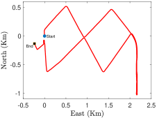
(b) trajectory on a road

Figure 6: Car and its trajectory (data credit: UniStrong Co., Ltd. and [29]).

The east axis (in the east-north-up coordinate) is investigated [29]. The RTAMSE performance against the values of $(\alpha,\beta)$ is shown in Fig. 7.

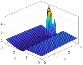
Figure 7: Averaged-RTAMSE performance of the $(\alpha,\beta)$-uncertainty-aware IMM filter, against the values of $(\alpha,\beta)$. The $(\alpha,\beta)$-uncertainty-aware IMM filter with $(\alpha,\beta)=(2,1.7)$ works best.

The results suggest that the $(\alpha,\beta)$-uncertainty-aware IMM (IMM-UA) filter with $(\alpha,\beta)=(2,1.7)$ works best, under which the tracking results (RTAMSE) are shown in Table I.

TABLE I: Tracking Results of The Car: $(\alpha,\beta)=(2,1.7)$

Filter	RTAMSE	Avg Time	Filter	RTAMSE	Avg Time
IMM	2.30	1.05e-05	IMM-UA	1.69	1.07e-05
Avg Time: Average Execution Time at each time step (unit: seconds).

From Table I, we can see that the value pair of $(\alpha,\beta)=(2,1.7)$ significantly reduces the tracking errors for the car. This value pair concentrates both the prior distribution (i.e., prior model weights) and the likelihood distribution (i.e., model likelihoods), which means that one of the three models in (30) dominates the rest two models most of the time. This implication coincides with our intuition from Fig. 6(b) that most of the time $k$, the model with $\mathrm{a}_{1,k}=0$ (i.e., constant velocity and straight-line trajectory) dominates the motion of the car.

III-C2 Track A Highly-Maneuvering Drone

We next track a highly-maneuvering drone that flies following round trajectories in the air over an open playground, with a flying speed of about $6$m/s during data collection. The drone and parts of its trajectory are shown in Fig. 8.

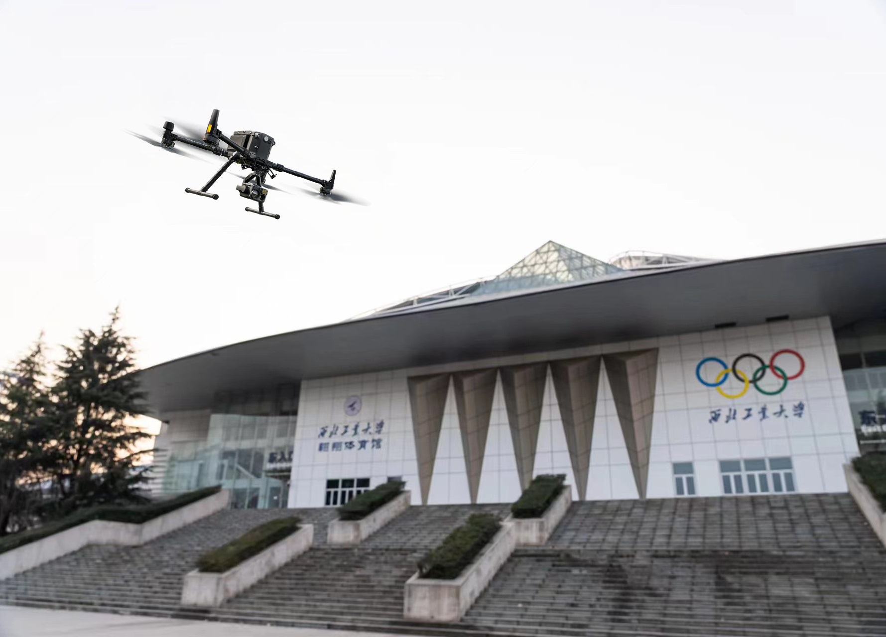
(a) drone

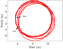
(b) trajectory (part)

Figure 8: Drone and its flying trajectory, starting from $10s$ and ending at $60s$ (data credit: Northwestern Polytechnical University and [29]).

The east axis (in the east-north-up coordinate) is investigated [29]. The RTAMSE performance against the values of $(\alpha,\beta)$ is shown in Fig. 9.

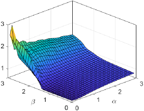
Figure 9: Averaged-RTAMSE performance of the $(\alpha,\beta)$-uncertainty-aware IMM filter, against the values of $(\alpha,\beta)$. The $(\alpha,\beta)$-uncertainty-aware IMM filter with $(\alpha,\beta)=(0.2,1.2)$ works best.

The results suggest that the $(\alpha,\beta)$-uncertainty-aware IMM filter with $(\alpha,\beta)=(0.2,1.2)$ works best, under which the tracking results (RTAMSE) are shown in Table II.

TABLE II: Tracking Results of The Drone: $(\alpha,\beta)=(0.2,1.2)$

Filter	RTAMSE	Avg Time	Filter	RTAMSE	Avg Time
IMM	0.77	2.71e-05	IMM-UA	0.60	2.85e-05
Avg Time: Average Execution Time at each time step (unit: seconds).

From Table II, we can see that the value pair of $(\alpha,\beta)=(0.2,1.2)$ significantly reduces the tracking errors for the drone. This value pair improves the entropy (i.e., the spread) of the likelihood distribution (i.e., the model likelihoods) and almost does not influence the prior distribution (i.e., the prior model weights because $\beta=1.2\approx 1$), which means that none of the three models in (30) dominates the rest two models and the model set in (30) is not complete (viz., more candidate values for $j_{k}$ and $\mathrm{a}_{j_{k},k}$ are expected; only three values are not sufficient). This implication coincides with our intuition from Fig. 8(b) that, since the drone highly maneuvers with acceleration quickly switching between positive values and negative values, there is no model that dominates the motion of the drone.

IV Conclusions

To combat the potential model misspecifications in prior distributions (i.e., prior belief) and/or data distributions (i.e., data evidence), this paper proposes to generalize the conventional Bayes’ rule to the uncertainty-aware Bayes’ rule. The uncertainty-aware Bayes’ rule balances the relative importance of the prior distribution and the likelihood distribution by simply taking the exponentiation of the prior distribution and the likelihood distribution. We show that this exponentiation operator essentially adjusts the entropy (i.e., the concentration, the spread) of the prior distribution and the likelihood distribution. Therefore, with different exponents, the prior distribution and/or the likelihood distribution can be upweighted (i.e., by reducing the entropy) or downweighted (i.e., by inflating the entropy) in computing the posterior. Compared to the existing maximum entropy scheme, the uncertainty-aware Bayes’ rule does not introduce much additional computational burden because the exponentiation operation is computationally light. In addition, compared to the existing maximum entropy scheme and $\alpha$-posterior scheme, the uncertainty-aware Bayes’ rule is able to combat the conservativeness (i.e., upweight the useful distributional information) of the employed prior distributions and the likelihood distributions. Simulated and real-world applications further advocate that both opportunism and conservatism are potentially useful in practice.

Future papers following this work are expected to investigate the posterior consistency and asymptotic properties (e.g., asymptotic normality or non-normality) of the derived uncertainty-aware Bayes’ rule, i.e., the $(\alpha,\beta)$-posterior; cf. [15, 6]. However, these problems are more mathematically statistical problems than theoretical signal processing problems, and therefore, we leave them to mathematical statisticians.

Appendix A Proof of Lemma 1

Proof:

According to the variational Bayesian interpretation of the posterior distribution $p(\bm{\theta}|\bm{y})$ in (1) (i.e., maximizing the evidence lower bound [30, p. 862]), $p(\bm{\theta}|\bm{y})$ solves

$$\min_{q(\bm{\theta})}\operatorname{KL}\left[{q(\bm{\theta})}\left\|{p(\bm{\theta})}\right.\right]+\mathbb{E}_{\bm{\theta}\sim q(\bm{\theta})}[-\ln{p(\bm{y}|\bm{\theta})}].$$

Let $C_{\bm{y}}\coloneqq\int p(\bm{y}|\bm{\theta})\mathrm{d}\bm{\theta}$. The above optimization problem is equivalent, in the sense of the same minimizer, to

$$\begin{array}[]{l}\displaystyle\min_{q(\bm{\theta})}\operatorname{KL}\left[{q(\bm{\theta})}\left\|{p(\bm{\theta})}\right.\right]+\mathbb{E}_{\bm{\theta}\sim q(\bm{\theta})}\left[-\ln\frac{p(\bm{y}|\bm{\theta})}{C_{\bm{y}}}\right],\\ \quad=\displaystyle\min_{q(\bm{\theta})}\operatorname{KL}\left[{q(\bm{\theta})}\left\|{p(\bm{\theta})}\right.\right]+\mathbb{E}_{\bm{\theta}\sim q(\bm{\theta})}[-\ln l(\bm{\theta})],\\ \quad=\displaystyle\min_{q(\bm{\theta})}\operatorname{KL}\left[{q(\bm{\theta})}\left\|{p(\bm{\theta})}\right.\right]+\operatorname{KL}\left[{q(\bm{\theta})}\left\|{l(\bm{\theta})}\right.\right]+\operatorname*{{Ent}}q(\bm{\theta}).\end{array}$$

This completes the proof. $\square$∎

Appendix B Proof of Theorem 1

Proof:

We have

$$\begin{array}[]{l}\displaystyle\min_{q(\bm{\theta})}\alpha_{1}\operatorname{KL}\left[{q(\bm{\theta})}\left\|{p(\bm{\theta})}\right.\right]+\alpha_{2}\operatorname{KL}\left[{q(\bm{\theta})}\left\|{l(\bm{\theta})}\right.\right]+\alpha_{3}\operatorname*{{Ent}}q(\bm{\theta})\\ \quad=\displaystyle\min_{q(\bm{\theta})}\int q(\bm{\theta})\ln\frac{q(\bm{\theta})}{p^{\alpha_{1}}(\bm{\theta})l^{\alpha_{2}}(\bm{\theta})q^{2\alpha_{3}}(\bm{\theta})}\mathrm{d}\bm{\theta}\\ \quad=\displaystyle\min_{q(\bm{\theta})}\int q(\bm{\theta})\ln\frac{q^{1-2\alpha_{3}}(\bm{\theta})}{p^{\alpha_{1}}(\bm{\theta})l^{\alpha_{2}}(\bm{\theta})}\mathrm{d}\bm{\theta}.\end{array}$$

When $\alpha_{3}=1/2$, any distribution supported on $\Theta^{*}$ solves the above optimization problem, where $\Theta^{*}$ contains all maximizers of $\ln[p^{\alpha_{1}}(\bm{\theta})l^{\alpha_{2}}(\bm{\theta})]$.

When $\alpha_{3}\neq 1/2$, the above optimization problem is equivalent to

$$(1-2\alpha_{3})\cdot\displaystyle\min_{q(\bm{\theta})}\int q(\bm{\theta})\ln\frac{q(\bm{\theta})}{p^{\frac{\alpha_{1}}{1-2\alpha_{3}}}(\bm{\theta})\cdot l^{\frac{\alpha_{2}}{1-2\alpha_{3}}}(\bm{\theta})}\mathrm{d}\bm{\theta},$$

which is further equivalent, in the sense of the same minimizer, to

$$\min_{q(\bm{\theta})}\operatorname{KL}\left[{q(\bm{\theta})}\left\|{\frac{p^{\frac{\alpha_{1}}{1-2\alpha_{3}}}(\bm{\theta})\cdot l^{\frac{\alpha_{2}}{1-2\alpha_{3}}}(\bm{\theta})}{C}}\right.\right],$$

where $C$ is the normalizer. This completes the proof. $\square$∎

Appendix C Proof of Theorem 2

Proof:

Let $C_{\alpha}\coloneqq\int h^{\alpha}(\bm{y})\mathrm{d}\bm{y}$. We have

$$\begin{array}[]{cl}\operatorname*{{Ent}}h^{(\alpha)}(\bm{y})&=\displaystyle\int\frac{h^{\alpha}(\bm{y})}{\int h^{\alpha}(\bm{y})\mathrm{d}\bm{y}}\cdot-\ln\frac{h^{\alpha}(\bm{y})}{\int h^{\alpha}(\bm{y})\mathrm{d}\bm{y}}\mathrm{d}\bm{y}\\ &=\displaystyle\frac{1}{C_{\alpha}}\int h^{\alpha}(\bm{y})\cdot\Big{[}-\ln h^{\alpha}(\bm{y})+\ln C_{\alpha}\Big{]}\mathrm{d}\bm{y}\\ &=\ln C_{\alpha}+\displaystyle\frac{\alpha}{C_{\alpha}}\int h^{\alpha}(\bm{y})\cdot-\ln h(\bm{y})\mathrm{d}\bm{y}.\end{array}$$

Therefore,

$$\begin{array}[]{l}\displaystyle\frac{\mathrm{d}\operatorname*{{Ent}}h^{(\alpha)}(\bm{y})}{\mathrm{d}\alpha}\propto\alpha\cdot\Bigg{\{}\left[\displaystyle\int h^{\alpha}(\bm{y})\ln h(\bm{y})\mathrm{d}\bm{y}\right]^{2}-\\ \quad\quad\quad\quad\quad\quad\displaystyle\int h^{\alpha}(\bm{y})\mathrm{d}\bm{y}\cdot\int h^{\alpha}(\bm{y})\ln h(\bm{y})\ln h(\bm{y})\mathrm{d}\bm{y}\Bigg{\}}.\end{array}$$

Since $h^{\alpha}(\bm{y})\geq 0$ for every $\alpha$ and $\bm{y}$, according to the Cauchy–Schwarz inequality, we have

$$\begin{array}[]{l}\displaystyle\int\left[\sqrt{h^{\alpha}(\bm{y})}\right]^{2}\mathrm{d}\bm{y}\int\left[\sqrt{h^{\alpha}(\bm{y})\cdot\ln h(\bm{y})\cdot\ln h(\bm{y})}\right]^{2}\mathrm{d}\bm{y}\\ \quad\quad\geq\left[\displaystyle\int\sqrt{h^{\alpha}(\bm{y})\cdot h^{\alpha}(\bm{y})\cdot\ln h(\bm{y})\cdot\ln h(\bm{y})}\mathrm{d}\bm{y}\right]^{2}\\ \quad\quad=\left[\displaystyle\int h^{\alpha}(\bm{y})\cdot\big{|}\ln h(\bm{y})\big{|}\mathrm{d}\bm{y}\right]^{2}\\ \quad\quad\geq\left[\displaystyle\int h^{\alpha}(\bm{y})\cdot\ln h(\bm{y})\mathrm{d}\bm{y}\right]^{2}.\end{array}$$

As a result,

$$\frac{\mathrm{d}\operatorname*{{Ent}}h^{(\alpha)}(\bm{y})}{\mathrm{d}\alpha}\begin{cases}\leq 0&\text{for }\alpha>0\\ \geq 0&\text{for }\alpha<0.\\ \end{cases}$$

The equality holds if and only if $h(\bm{y})$ is a uniform distribution. This completes the proof. $\square$∎

Appendix D Proof of Theorem 3

Before proving Theorem 3, we prepare with the following lemma. For discrete distributions, the statement of the lemma is obvious, but for continuous distributions, we need much more effort to prove it.

Lemma 2

If $\alpha>1$, then

$$\int h^{(\alpha)}(\bm{y})\ln h(\bm{y})\mathrm{d}\bm{y}-\int h(\bm{y})\ln h(\bm{y})\mathrm{d}\bm{y}>0;$$

if $\alpha<1$, then

$$\int h^{(\alpha)}(\bm{y})\ln h(\bm{y})\mathrm{d}\bm{y}-\int h(\bm{y})\ln h(\bm{y})\mathrm{d}\bm{y}<0.$$

Proof:

Let $C_{\alpha}\coloneqq\int h^{\alpha}(\bm{y})\mathrm{d}\bm{y}$. Jeffrey’s divergence (NB: it is symmetric) between ${h(\bm{y})}$ and ${h^{(\alpha)}(\bm{y})}$ can be given as

$$\begin{array}[]{l}\operatorname{KL}\left[{h^{(\alpha)}(\bm{y})}\left\|{h(\bm{y})}\right.\right]+\operatorname{KL}\left[{h(\bm{y})}\left\|{h^{(\alpha)}(\bm{y})}\right.\right]\\ \quad=\displaystyle\int\frac{h^{\alpha}(\bm{y})}{C_{\alpha}}\ln\frac{h^{\alpha}(\bm{y})}{C_{\alpha}\cdot h(\bm{y})}\mathrm{d}\bm{y}+\displaystyle\int h(\bm{y})\ln\frac{C_{\alpha}\cdot h(\bm{y})}{h^{\alpha}(\bm{y})}\mathrm{d}\bm{y}\\ \quad=\displaystyle\frac{1}{C_{\alpha}}\Big{[}\int h^{\alpha}(\bm{y})\ln h^{\alpha}(\bm{y})\mathrm{d}\bm{y}-\par\displaystyle\int h^{\alpha}(\bm{y})\ln C_{\alpha}\mathrm{d}\bm{y}-\\ \quad\quad\quad\displaystyle\int h^{\alpha}(\bm{y})\ln h(\bm{y})\mathrm{d}\bm{y}\par\Big{]}+\Big{[}\displaystyle\int h(\bm{y})\ln C_{\alpha}\mathrm{d}\bm{y}+\\ \quad\quad\quad\displaystyle\int h(\bm{y})\ln h(\bm{y})\mathrm{d}\bm{y}-\int h(\bm{y})\ln{h^{\alpha}(\bm{y})}\mathrm{d}\bm{y}\Big{]}\\ \quad=\displaystyle\frac{\alpha-1}{C_{\alpha}}\int h^{\alpha}(\bm{y})\ln h(\bm{y})\mathrm{d}\bm{y}-\ln C_{\alpha}+\ln C_{\alpha}+\\ \quad\quad\quad\displaystyle(1-\alpha)\int h(\bm{y})\ln h(\bm{y})\mathrm{d}\bm{y}\\ \quad=(\alpha-1)\Big{[}\displaystyle\displaystyle\int h^{(\alpha)}(\bm{y})\ln h(\bm{y})\mathrm{d}\bm{y}-\int h(\bm{y})\ln h(\bm{y})\mathrm{d}\bm{y}\Big{]}\\ \quad\geq 0.\end{array}$$

The equality holds if and only if $\alpha=1$. This completes the proof. $\square$∎

Now we proceed to the proof of Theorem 3.

Proof:

Let $C_{\alpha}\coloneqq\int h^{\alpha}(\bm{y})\mathrm{d}\bm{y}$. We have

$$\begin{array}[]{l}\operatorname{KL}\left[{h(\bm{y})}\left\|{h^{(\alpha)}(\bm{y})}\right.\right]\\ \quad\quad=\displaystyle\int h(\bm{y})\ln\frac{h(\bm{y})}{h^{(\alpha)}(\bm{y})}\mathrm{d}\bm{y}\\ \quad\quad=\displaystyle\int h(\bm{y})\ln\frac{C\cdot h(\bm{y})}{h^{\alpha}(\bm{y})}\mathrm{d}\bm{y}\\ \quad\quad=\ln C+(\alpha-1)\operatorname*{{Ent}}h(\bm{y}).\end{array}$$

Therefore,

$$\begin{array}[]{l}\displaystyle\frac{\mathrm{d}\operatorname{KL}\left[{h(\bm{y})}\left\|{h^{(\alpha)}(\bm{y})}\right.\right]}{\mathrm{d}\alpha}\\ \quad\quad=\displaystyle\int h^{(\alpha)}(\bm{y})\ln h(\bm{y})\mathrm{d}\bm{y}+\operatorname*{{Ent}}h(\bm{y})\\ \quad\quad=\displaystyle\int h^{(\alpha)}(\bm{y})\ln h(\bm{y})\mathrm{d}\bm{y}-\int h(\bm{y})\ln h(\bm{y})\mathrm{d}\bm{y}.\end{array}$$

Then, by Lemma 2, the monotonicity is immediate.

In addition,

$$\begin{array}[]{l}\displaystyle\frac{\mathrm{d}^{2}\operatorname{KL}\left[{h(\bm{y})}\left\|{h^{(\alpha)}(\bm{y})}\right.\right]}{\mathrm{d}^{2}\alpha}\\ \quad=\displaystyle\frac{1}{C^{2}_{\alpha}}\Bigg{\{}\displaystyle\int h^{\alpha}(\bm{y})\mathrm{d}\bm{y}\cdot\int h^{\alpha}(\bm{y})\ln h(\bm{y})\ln h(\bm{y})\mathrm{d}\bm{y}-\\ \quad\quad\quad\quad\quad\quad\left[\displaystyle\int h^{\alpha}(\bm{y})\ln h(\bm{y})\mathrm{d}\bm{y}\right]^{2}\Bigg{\}}\\ \quad\geq 0.\end{array}$$

The last inequality is due to the Cauchy–Schwarz inequality; see Appendix C. This completes the proof. $\square$∎

Dr. Shixiong Wang received the B.Eng. degree in detection, guidance, and control technology, and the M.Eng. degree in systems and control engineering from the School of Electronics and Information, Northwestern Polytechnical University, China, in 2016 and 2018, respectively. He received his Ph.D. degree from the Department of Industrial Systems Engineering and Management, National University of Singapore, Singapore, in 2022. He is currently a Postdoctoral Research Associate with the Intelligent Transmission and Processing Laboratory, Imperial College London, London, United Kingdom, from May 2023. He was a Postdoctoral Research Fellow with the Institute of Data Science, National University of Singapore, Singapore, from March 2022 to March 2023. His research interest includes statistics and optimization theories with applications in signal processing (especially optimal estimation theory), machine learning (especially generalization error theory), and control technology.

References

- [1] R. van de Schoot, S. Depaoli, R. King, B. Kramer, K. Märtens, M. G. Tadesse, M. Vannucci, A. Gelman, D. Veen, J. Willemsen et al., “Bayesian statistics and modelling,” Nature Reviews Methods Primers, vol. 1, no. 1, p. 1, 2021.
- [2] J. O. Berger, “An overview of robust Bayesian analysis,” Test, vol. 3, no. 1, pp. 5–124, 1994.
- [3] D. R. Insua and F. Ruggeri, Robust Bayesian Analysis. New York: Springer, 2000.
- [4] F. Ruggeri, D. R. Insua, and J. Martín, “Robust Bayesian analysis,” Handbook of Statistics, vol. 25, pp. 623–667, 2005.
- [5] A. Gelman, J. B. Carlin, H. S. Stern, and D. B. Rubin, Bayesian Data Analysis, 3rd ed. Chapman and Hall/CRC, 2013.
- [6] M. A. Medina, J. L. M. Olea, C. Rush, and A. Velez, “On the robustness to misspecification of -posteriors and their variational approximations,” The Journal of Machine Learning Research, vol. 23, no. 1, pp. 6579–6629, 2022.
- [7] I. R. Petersen and A. V. Savkin, Robust Kalman Filtering for Signals and Systems with Large Uncertainties. Springer Science & Business Media, 1999.
- [8] A. M. Zoubir, V. Koivunen, E. Ollila, and M. Muma, Robust Statistics for Signal Processing. Cambridge University Press, 2018.
- [9] Y. S. Shmaliy, F. Lehmann, S. Zhao, and C. K. Ahn, “Comparing Robustness of the Kalman, , and UFIR Filters,” IEEE Transactions on Signal Processing, vol. 66, no. 13, pp. 3447–3458, 2018.
- [10] S. Wang, “Distributionally Robust State Estimation,” Ph.D. dissertation, National University of Singapore, 2022.
- [11] P. J. Huber and E. M. Ronchetti, Robust Statistics, 2nd ed. John Wiley & Sons Hoboken, NJ, USA, 2009.
- [12] P. J. Huber, “Robust estimation of a location parameter,” The Annals of Mathematical Statistics, vol. 35, no. 1, pp. 73–101, 1964. [Online]. Available: http://www.jstor.org/stable/2238020
- [13] F. R. Hampel, “The influence curve and its role in robust estimation,” Journal of the American Statistical Association, vol. 69, no. 346, pp. 383–393, 1974.
- [14] S. Ghosal and A. Van der Vaart, Fundamentals of Nonparametric Bayesian inference. Cambridge University Press, 2017, vol. 44.
- [15] P. Alquier and J. Ridgway, “Concentration of tempered posteriors and of their variational approximations,” The Annals of Statistics, vol. 48, no. 3, pp. 1475–1497, 2020. [Online]. Available: https://doi.org/10.1214/19-AOS1855
- [16] S. Wang, “Distributionally robust state estimation for nonlinear systems,” IEEE Transactions on Signal Processing, vol. 70, pp. 4408–4423, 2022.
- [17] M. J. Rufo, J. Martín, and C. J. Pérez, “Log-Linear Pool to Combine Prior Distributions: A Suggestion for a Calibration-Based Approach,” Bayesian Analysis, vol. 7, no. 2, pp. 411 – 438, 2012. [Online]. Available: https://doi.org/10.1214/12-BA714
- [18] G. Koliander, Y. El-Laham, P. M. Djurić, and F. Hlawatsch, “Fusion of probability density functions,” Proceedings of the IEEE, vol. 110, no. 4, pp. 404–453, 2022.
- [19] S. Wang and Z.-S. Ye, “Distributionally robust state estimation for linear systems subject to uncertainty and outlier,” IEEE Transactions on Signal Processing, vol. 70, pp. 452–467, 2021.
- [20] B. D. Anderson and J. B. Moore, Optimal Filtering. Prentice-Hall, N.J., 1979.
- [21] S. Wang, Z. Wu, and A. Lim, “Robust state estimation for linear systems under distributional uncertainty,” IEEE Transactions on Signal Processing, vol. 69, pp. 5963–5978, 2021.
- [22] M. S. Arulampalam, S. Maskell, N. Gordon, and T. Clapp, “A tutorial on particle filters for online nonlinear/non-Gaussian Bayesian tracking,” IEEE Transactions on Signal Processing, vol. 50, no. 2, pp. 174–188, 2002.
- [23] B. P. Carlin, N. G. Polson, and D. S. Stoffer, “A monte carlo approach to nonnormal and nonlinear state-space modeling,” Journal of the American Statistical Association, vol. 87, no. 418, pp. 493–500, 1992.
- [24] H. A. Blom and Y. Bar-Shalom, “The interacting multiple model algorithm for systems with Markovian switching coefficients,” IEEE Transactions on Automatic Control, vol. 33, no. 8, pp. 780–783, 1988.
- [25] Y. Bar-Shalom, S. Challa, and H. A. Blom, “Imm estimator versus optimal estimator for hybrid systems,” IEEE Transactions on Aerospace and Electronic Systems, vol. 41, no. 3, pp. 986–991, 2005.
- [26] X. R. Li and V. P. Jilkov, “Survey of maneuvering target tracking. part i. dynamic models,” IEEE Transactions on Aerospace and Electronic Systems, vol. 39, no. 4, pp. 1333–1364, 2003.
- [27] V. P. Jilkov and X. R. Li, “Online Bayesian estimation of transition probabilities for markovian jump systems,” IEEE Transactions on Signal Processing, vol. 52, no. 6, pp. 1620–1630, 2004.
- [28] S. Zhao and F. Liu, “Recursive estimation for Markov jump linear systems with unknown transition probabilities: A compensation approach,” Journal of the Franklin Institute, vol. 353, no. 7, pp. 1494–1517, 2016.
- [29] S. Wang, “Distributionally robust state estimation for jump linear systems,” IEEE Transactions on Signal Processing, pp. 3835–3851, 2023.
- [30] D. M. Blei, A. Kucukelbir, and J. D. McAuliffe, “Variational inference: A review for statisticians,” Journal of the American Statistical Association, vol. 112, no. 518, pp. 859–877, 2017.