Conditional no-jump dynamics of non-interacting quantum chains

Michele Coppola michele.coppola@univ-lorraine.fr LPCT, Université de Lorraine, CNRS, F-54000 Nancy, France    Dragi Karevski dragi.karevski@univ-lorraine.fr LPCT, Université de Lorraine, CNRS, F-54000 Nancy, France    Gabriel T. Landi gabriel.landi@rochester.edu Department of Physics and Astronomy, University of Rochester, Rochester, New York 14627, USA
Abstract

We analyze the open dynamics of quantum systems conditioned on no jumps being detected. We first obtain general results relating the no-jump probability and the waiting-time distributions to the conditional evolution of specific system observables. These results are applied to single-qubit models, whose conditional dynamics is quite involved and shows a rich set of physical behaviors. Furthermore, we obtain general expressions for the no-jump dynamics of non-interacting fermionic-bosonic chains undergoing Gaussian-preserving dynamics. We show that the conditional dynamics is determined by a non-linear Riccati-type differential equation for the correlation matrix. Finally, we apply our results to chains of hopping particles under inhomogeneous jump rates and boundary driven systems in presence of pairing terms.

I Introduction

Non-equilibrium open quantum systems continue to raise many physical challenges. In this respect, we may quote the transport phenomena in driven quantum chains, where a non-unitary dynamics is generated by the coupling with external reservoirs (e.g. Lindblad baths)  landi2022nonequilibrium. The quantum trajectory techniques represent a simple tool to access the non-unitary evolution by stochastic averages over single trajectories evolving in time as pure states daley2014quantum; wiseman1996quantum; dalibard1992wave; gardiner1992wave; carollo2019unraveling. The evolution of any trajectory is generated by a non-Hermitian effective Hamiltonian, perturbed by the so-called quantum jumps appearing stochastically in time with characteristic rates. The complete statistics of jumps occurring in time, as well as their nature, is captured by the theory of Full Counting Statistics levitov1993charge; esposito2007fluctuation; esposito2009nonequilibrium; landi2023current. Connected to these concepts, the no-jump probabilities and the waiting-time distributions (WTDs) brandes2008waiting; landi2021waiting; landi2023current represent a powerful theoretical probe to investigate the interplay between non-Hermitian dynamics and jump events.

In Ref. landi2021waiting one of us approached the problem of computing the WTDs for boundary driven quadratic fermion chains, subject to single-particle gain-loss processes. In that case, quantum jumps may be pictorially seen as the action of some detectors monitoring the exchange of particles between the system and the external environment. In this paper we expand on those preliminary results in various ways. First, we generalize the boundary-driven setup by keeping the coupling with the bath(s) along all the sites of the chain, where the coupling amplitude is modulated by inhomogeneous jump rates. Second, we introduce non-ideal monitoring efficiencies, by assigning each jump channel j𝑗j a real coefficient Λj[0,1]subscriptΛ𝑗01\Lambda_{j}\in[0,1], with Λj=1subscriptΛ𝑗1\Lambda_{j}=1 for perfect efficiency and Λj=0subscriptΛ𝑗0\Lambda_{j}=0 when the channel is not monitored at all. Therefore, our setting reduces to the case studied into Ref. landi2021waiting for the specific choice Λj=1subscriptΛ𝑗1\Lambda_{j}=1. In other terms, we extend the view to the missed detection of some jump events due the intrinsic imperfection of the monitoring apparatus. This study is clearly useful for experimentalists, where the efficiency of the monitoring apparatus is not ideal and may change with the work conditions. The main purpose of this paper is to compute the conditional no-jump dynamics of the density operator, which is the time evolution conditioned on no jumps being detected. In this view, the waiting time distribution Wk(t)subscript𝑊𝑘𝑡W_{k}(t) is the probability distribution to detect the first jump in channel k𝑘k after time t𝑡t. Third, our efforts will also be addressed to the no-jump probability Pno(t)subscript𝑃no𝑡P_{\rm no}(t), which is the probability to detect the first jump at time t𝑡t. Fourth, we also derive results for particle non-conserving Hamiltonian operators and, fifth, we study both bosonic and fermionic cases. In conclusion, this work aims to be a complete study of the no-jump dynamics of non-interacting quantum chains.

In Sec. II we define the Lindblad evolution and the no-jump dynamics, characterized by damping rates and monitoring efficiencies. We introduce the no-jump probability and the WTDs, generalizing the definitions into Ref. landi2021waiting for non-ideal efficiencies. In Sec. III, we study two simple applications involving a single qubit, either incoherently or coherently driven. In Sec. IV we approach the many-body problem of a chain of hopping particles with single particle gain-loss processes. Thanks to the Gaussian ansatz, the no-jump dynamics turns to be governed by a Riccati-type differential equation for the correlation matrix. As an application (Sec. VI), we study a chain of hopping fermions with specific absorption-emission profiles. In Sec. VII and Sec. VIII, we also derive the no-jump dynamics for particle non-conserving Hamiltonians (pairing terms). As an example, we consider the no-jump dynamics of a 222-site boundary driven system (Sec. IX). Our main findings are summarized in Sec. X, where we draw some future perspectives. Several appendices contain technical details and background.

II General framework

Refer to caption
Figure 1: Example of a quantum jump trajectory, as viewed from the perspective of a pictorial system observable. Abrupt jumps occur at random times and, in between, the observable evolves smoothly, governed by the so-called no-jump conditional evolution.

Let ρ𝜌\rho be the density operator of a quantum system whose dynamics is generated by the Liouvillian (ρ)𝜌\mathcal{L}(\rho)

dρdt=(ρ)=i[H,ρ]+𝒟(ρ),𝑑𝜌𝑑𝑡𝜌𝑖𝐻𝜌𝒟𝜌\frac{d\rho}{dt}=\mathcal{L}(\rho)=-i[H,\rho]+\mathcal{D}(\rho), (II.1)

where H𝐻H denotes the Hamiltonian and 𝒟(ρ)𝒟𝜌\mathcal{D}(\rho) is the dissipator

𝒟(ρ)=kDρ[Lk]=k(LkρLk12{LkLk,ρ}),𝒟𝜌subscript𝑘subscript𝐷𝜌delimited-[]subscript𝐿𝑘subscript𝑘subscript𝐿𝑘𝜌superscriptsubscript𝐿𝑘12superscriptsubscript𝐿𝑘subscript𝐿𝑘𝜌\mathcal{D}(\rho)=\sum_{k}D_{\rho}[L_{k}]=\sum_{k}\left(L_{k}\rho L_{k}^{\dagger}-\frac{1}{2}\{L_{k}^{\dagger}L_{k},\rho\}\right), (II.2)

characterized by a generic set of Lindblad jump operators Lksubscript𝐿𝑘L_{k}.

In the quantum jump unravelling wiseman1996quantum the terms LkρLksubscript𝐿𝑘𝜌superscriptsubscript𝐿𝑘L_{k}\rho L_{k}^{\dagger} represent quantum jumps, so that the dynamics can be viewed as a series of discrete jumps, followed by a smooth no-jump evolution. (Fig. 1). Each Lindblad operator corresponds to a different channel where the jump might occur, which is signaled by a click in a classical detector. In this work, we assume that one can independently choose to measure each Lksubscript𝐿𝑘L_{k} with different efficiencies ΛksubscriptΛ𝑘\Lambda_{k}, with Λk=1subscriptΛ𝑘1\Lambda_{k}=1 being perfect monitoring and Λk=0subscriptΛ𝑘0\Lambda_{k}=0 meaning that channel is not monitored at all. We now split Eq. (II.1) as

=0+1,subscript0subscript1\mathcal{L}=\mathcal{L}_{0}+\mathcal{L}_{1}, (II.3)

where

1(ρ)subscript1𝜌\displaystyle\mathcal{L}_{1}(\rho) =k𝒥kρ=kΛkLkρLk,absentsubscript𝑘subscript𝒥𝑘𝜌subscript𝑘subscriptΛ𝑘subscript𝐿𝑘𝜌superscriptsubscript𝐿𝑘\displaystyle=\sum_{k}\mathcal{J}_{k}\rho=\sum_{k}\Lambda_{k}L_{k}\rho L_{k}^{\dagger}, (II.4)

with each jump channel specified by the super-operator 𝒥ksubscript𝒥𝑘\mathcal{J}_{k}. The conditional no-jump operator is

0(ρ)=i[H,ρ]+k[(1Λk)LkρLk12{LkLk,ρ}].subscript0𝜌𝑖𝐻𝜌subscript𝑘delimited-[]1subscriptΛ𝑘subscript𝐿𝑘𝜌superscriptsubscript𝐿𝑘12superscriptsubscript𝐿𝑘subscript𝐿𝑘𝜌\mathcal{L}_{0}(\rho)=-i[H,\rho]+\sum_{k}\left[(1-\Lambda_{k})L_{k}\rho L_{k}^{\dagger}-\frac{1}{2}\{L_{k}^{\dagger}L_{k},\rho\}\right]. (II.5)

If all jumps are perfectly monitored, Λk=1subscriptΛ𝑘1\Lambda_{k}=1 kfor-all𝑘\forall k, then 0subscript0\mathcal{L}_{0} can also be written as

0(ρ)=i(HeρρHe),subscript0𝜌𝑖subscript𝐻e𝜌𝜌superscriptsubscript𝐻e\mathcal{L}_{0}(\rho)=-i\Big{(}H_{\rm e}\rho-\rho H_{\rm e}^{\dagger}\Big{)}, (II.6)

where

He=Hi2kLkLk,subscript𝐻𝑒𝐻𝑖2subscript𝑘superscriptsubscript𝐿𝑘subscript𝐿𝑘H_{e}=H-\frac{i}{2}\sum_{k}L_{k}^{\dagger}L_{k}, (II.7)

is a kind of non-Hermitian Hamiltonian.

The solution ρ(t)=etρ0𝜌𝑡superscript𝑒𝑡subscript𝜌0\rho(t)=e^{\mathcal{L}t}\rho_{0}, called the unconditional dynamics (since it is ignorant about whether any jumps occurred or not) can be expanded in a Dyson series as

ρ(t)𝜌𝑡\displaystyle\rho(t) =e0tρ0+0t𝑑t1e0(tt1)1e0t1ρ0absentsuperscript𝑒subscript0𝑡subscript𝜌0superscriptsubscript0𝑡differential-dsubscript𝑡1superscript𝑒subscript0𝑡subscript𝑡1subscript1superscript𝑒subscript0subscript𝑡1subscript𝜌0\displaystyle=e^{\mathcal{L}_{0}t}\rho_{0}+\int\limits_{0}^{t}dt_{1}e^{\mathcal{L}_{0}(t-t_{1})}\mathcal{L}_{1}e^{\mathcal{L}_{0}t_{1}}\rho_{0}
+0t𝑑t20t2𝑑t1e0(tt2)1e0(t2t1)1e0t1ρ0+,superscriptsubscript0𝑡differential-dsubscript𝑡2superscriptsubscript0subscript𝑡2differential-dsubscript𝑡1superscript𝑒subscript0𝑡subscript𝑡2subscript1superscript𝑒subscript0subscript𝑡2subscript𝑡1subscript1superscript𝑒subscript0subscript𝑡1subscript𝜌0\displaystyle+\int\limits_{0}^{t}dt_{2}\int\limits_{0}^{t_{2}}dt_{1}e^{\mathcal{L}_{0}(t-t_{2})}\mathcal{L}_{1}e^{\mathcal{L}_{0}(t_{2}-t_{1})}\mathcal{L}_{1}e^{\mathcal{L}_{0}t_{1}}\rho_{0}+\ldots, (II.8)

where ρ(t=0)=ρ0𝜌𝑡0subscript𝜌0\rho(t=0)=\rho_{0}. The first term e0tρ0superscript𝑒subscript0𝑡subscript𝜌0e^{\mathcal{L}_{0}t}\rho_{0} is the evolution conditioned on having no jumps up to time t𝑡t, the second is conditioned on having exactly one jump at time t1subscript𝑡1t_{1}, etc plenio1998quantum; landi2022nonequilibrium. Let us focus on the first term, i.e. the no-jump conditional dynamics. Since 0subscript0\mathcal{L}_{0} is not a proper Liouvillian, the evolved state e0tρ0superscript𝑒subscript0𝑡subscript𝜌0e^{\mathcal{L}_{0}t}\rho_{0} is not normalized. We define the unnormalized density matrix

ρ~no(t)=e0tρ0,dρ~nodt=0(ρ~no).formulae-sequencesubscript~𝜌no𝑡superscript𝑒subscript0𝑡subscript𝜌0𝑑subscript~𝜌no𝑑𝑡subscript0subscript~𝜌no\tilde{\rho}_{\rm no}(t)=e^{\mathcal{L}_{0}t}\rho_{0},\qquad\frac{d\tilde{\rho}_{\rm no}}{dt}=\mathcal{L}_{0}(\tilde{\rho}_{\rm no}). (II.9)

If all channels are monitored (Λk=1subscriptΛ𝑘1\Lambda_{k}=1), this reduces to

ρ~no(t)=eiHetρ0eiHet,subscript~𝜌no𝑡superscript𝑒𝑖subscript𝐻𝑒𝑡subscript𝜌0superscript𝑒𝑖superscriptsubscript𝐻𝑒𝑡\tilde{\rho}_{\rm no}(t)=e^{-iH_{e}t}\rho_{0}e^{iH_{e}^{\dagger}t}, (II.10)

which represents a non-Hermitian dynamics. The conditional evolution is indeed a very natural way of implementing non-Hermitian physics Purkayastha2022. The trace of ρ~no(t)subscript~𝜌no𝑡\tilde{\rho}_{\rm no}(t) is precisely the probability that no jump occurs between [0,t]0𝑡[0,t]:

Pno(t)=trρ~no(t).subscript𝑃no𝑡tracesubscript~𝜌no𝑡P_{\rm no}(t)=\tr\leavevmode\nobreak\ \tilde{\rho}_{\rm no}(t). (II.11)

The corresponding normalized conditional state is

ρno(t)=ρ~no(t)Pno(t).subscript𝜌no𝑡subscript~𝜌no𝑡subscript𝑃no𝑡{\rho}_{\rm no}(t)=\frac{\tilde{\rho}_{\rm no}(t)}{P_{\rm no}(t)}. (II.12)

The probability Pno(t)subscript𝑃no𝑡P_{\rm no}(t) satisfies Pno(0)=1subscript𝑃no01P_{\rm no}(0)=1. In the limit t𝑡t\to\infty, it may either tend to zero or to a finite value. When Pno()=0subscript𝑃no0P_{\rm no}(\infty)=0 it means a jump must eventually occur. Conversely, Pno()0subscript𝑃no0P_{\rm no}(\infty)\neq 0 means it might never do. This happens when the system has a dark subspace, which is immune to the dissipator in (II.2).

The unconditional evolution of any system observable 𝒪𝒪\mathcal{O} can be obtained from Eq. (II.1) and reads

d𝒪dt=(𝒪),𝑑delimited-⟨⟩𝒪𝑑𝑡delimited-⟨⟩superscript𝒪\frac{d\langle\mathcal{O}\rangle}{dt}=\langle\mathcal{L}^{\dagger}(\mathcal{O})\rangle, (II.13)

where

(𝒪)=superscript𝒪absent\displaystyle\mathcal{L}^{\dagger}(\mathcal{O})= i[H,𝒪]+k[Lk𝒪Lk12{LkLk,𝒪}],𝑖𝐻𝒪subscript𝑘delimited-[]superscriptsubscript𝐿𝑘𝒪subscript𝐿𝑘12superscriptsubscript𝐿𝑘subscript𝐿𝑘𝒪\displaystyle i[H,\mathcal{O}]+\sum_{k}\left[L_{k}^{\dagger}\mathcal{O}L_{k}-\frac{1}{2}\{L_{k}^{\dagger}L_{k},\mathcal{O}\}\right], (II.14)

is the adjoint dissipator and delimited-⟨⟩\langle\ldots\rangle denotes the expectation value over the unconditional state ρ(t)𝜌𝑡\rho(t). We can also write down a similar evolution equation for the conditional expectation value

𝒪no:=tr(𝒪ρno(t))=tr(𝒪ρ~no(t))Pno(t),assignsubscriptdelimited-⟨⟩𝒪notrace𝒪subscript𝜌no𝑡trace𝒪subscript~𝜌no𝑡subscript𝑃no𝑡\langle\mathcal{O}\rangle_{\rm no}:=\tr(\mathcal{O}{\rho}_{\rm no}(t))=\frac{\tr(\mathcal{O}\tilde{\rho}_{\rm no}(t))}{P_{\rm no}(t)}, (II.15)

i.e., properly normalized. Using Eq. (II.5) and taking into account the time-dependence of Pno(t)subscript𝑃no𝑡P_{\rm no}(t), one finds

d𝒪nodt=𝑑subscriptdelimited-⟨⟩𝒪no𝑑𝑡absent\displaystyle\frac{d\langle\mathcal{O}\rangle_{\rm no}}{dt}= (𝒪)nosubscriptdelimited-⟨⟩superscript𝒪no\displaystyle\,\langle\mathcal{L}^{\dagger}(\mathcal{O})\rangle_{\rm no}
kΛk[Lk𝒪Lkno𝒪noLkLkno].subscript𝑘subscriptΛ𝑘delimited-[]subscriptdelimited-⟨⟩superscriptsubscript𝐿𝑘𝒪subscript𝐿𝑘nosubscriptdelimited-⟨⟩𝒪nosubscriptdelimited-⟨⟩superscriptsubscript𝐿𝑘subscript𝐿𝑘no\displaystyle-\sum_{k}\Lambda_{k}\left[\langle L_{k}^{\dagger}\mathcal{O}L_{k}\rangle_{\rm no}-\langle\mathcal{O}\rangle_{\rm no}\langle L_{k}^{\dagger}L_{k}\rangle_{\rm no}\right]. (II.16)

The first term is the same as in the unconditional evolution (II.13), while the others are new contributions stemming from monitoring the jumps.

Next we differentiate Eq. (II.11), substituting 0=1subscript0subscript1\mathcal{L}_{0}=\mathcal{L}-\mathcal{L}_{1}. Since \mathcal{L} is traceless, using Eq. (II.4) we find

dPnodt=β(t)Pno,𝑑subscript𝑃no𝑑𝑡𝛽𝑡subscript𝑃no\frac{d{P}_{\rm no}}{dt}=-\beta(t)\,P_{\rm no}, (II.17)

where

β(t):=tr(1(ρno))=kΛkLkLkno(t).assign𝛽𝑡tracesubscript1subscript𝜌nosubscript𝑘subscriptΛ𝑘subscriptdelimited-⟨⟩superscriptsubscript𝐿𝑘subscript𝐿𝑘no𝑡\beta(t):=\tr\left(\mathcal{L}_{1}(\rho_{\rm no})\right)=\sum_{k}\Lambda_{k}\langle L_{k}^{\dagger}L_{k}\rangle_{\rm no}(t). (II.18)

The solution of Eq. (II.17) is

Pno(t)=exp{0t𝑑tβ(t)}.subscript𝑃no𝑡superscriptsubscript0𝑡differential-dsuperscript𝑡𝛽superscript𝑡P_{\rm no}(t)=\exp\left\{-\int\limits_{0}^{t}dt^{\prime}\beta(t^{\prime})\right\}. (II.19)

This result relates the no-jump probability with the expectation values of the jump operators. It therefore shows that it is not necessary to compute the full state ρnosubscript𝜌no\rho_{\rm no} to obtain Pnosubscript𝑃noP_{\rm no}, but instead we only need LkLknosubscriptdelimited-⟨⟩superscriptsubscript𝐿𝑘subscript𝐿𝑘no\langle L_{k}^{\dagger}L_{k}\rangle_{\rm no}, which can be obtained from Eq. (II). Eq. (II.19) also establishes a criteria for the existence or not of a dark subspace. If β=limtβ(t)superscript𝛽subscript𝑡𝛽𝑡\beta^{\infty}=\lim_{t\to\infty}\beta(t) then, in the long-time limit, the no-jump probability behaves as Pno(t)exp(βt)similar-tosubscript𝑃no𝑡superscript𝛽𝑡P_{\rm no}(t)\sim\exp{-\beta^{\infty}t}. Thus, limtPno(t)=0subscript𝑡subscript𝑃no𝑡0\lim_{t\to\infty}P_{\rm no}(t)=0 if at least one term ΛkLkLkno0subscriptΛ𝑘superscriptsubscriptdelimited-⟨⟩superscriptsubscript𝐿𝑘subscript𝐿𝑘no0\Lambda_{k}\langle L_{k}^{\dagger}L_{k}\rangle_{\rm no}^{\infty}\neq 0. The existence of dark subspaces is thus not only a property of the master equation (II.1), but also of what is monitored (i.e., the ΛksubscriptΛ𝑘\Lambda_{k}). As a sanity check, if nothing is monitored (Λk=0ksubscriptΛ𝑘0for-all𝑘\Lambda_{k}=0\leavevmode\nobreak\ \forall k) we simply find Pno(t)=1subscript𝑃no𝑡1P_{\rm no}(t)=1.

Computing the no-jump probability Pno(t)subscript𝑃no𝑡P_{\rm no}(t) also plays a key role in the study of the WTDs. The waiting-time distribution Wk(t)subscript𝑊𝑘𝑡W_{k}(t) is defined as

Wk(t)subscript𝑊𝑘𝑡\displaystyle W_{k}(t) :=tr{𝒥ke0t(ρ0)},assignabsenttracesubscript𝒥𝑘superscript𝑒subscript0𝑡subscript𝜌0\displaystyle:=\tr\{\mathcal{J}_{k}e^{\mathcal{L}_{0}t}({\rho}_{0})\Big{\}},
=Pno(t)tr{𝒥kρno(t)}.absentsubscript𝑃no𝑡tracesubscript𝒥𝑘subscript𝜌no𝑡\displaystyle=P_{\rm no}(t)\tr\{\mathcal{J}_{k}\>{\rho}_{\rm no}(t)\Big{\}}. (II.20)
=ΛkPno(t)LkLkno(t).absentsubscriptΛ𝑘subscript𝑃no𝑡subscriptdelimited-⟨⟩superscriptsubscript𝐿𝑘subscript𝐿𝑘no𝑡\displaystyle=\Lambda_{k}P_{\rm no}(t)\langle L_{k}^{\dagger}L_{k}\rangle_{\rm no}(t). (II.21)

which is the probability distribution to detect the first jump in the channel k𝑘k at time t𝑡t. The WTDs are normalized as

k0Wk(t)𝑑t=1.subscript𝑘superscriptsubscript0subscript𝑊𝑘𝑡differential-d𝑡1\sum_{k}\int_{0}^{\infty}W_{k}(t)\>dt=1. (II.22)

From these results we therefore reach the conclusion that both Pno(t)subscript𝑃no𝑡P_{\rm no}(t) and Wk(t)subscript𝑊𝑘𝑡W_{k}(t) can be computed by the conditional evolution of the Lindblad jump operators LkLkno(t)subscriptdelimited-⟨⟩superscriptsubscript𝐿𝑘subscript𝐿𝑘no𝑡\langle L_{k}^{\dagger}L_{k}\rangle_{\rm no}(t).

III Qubit example

Consider a single qubit with Rabi drive H=Ω2σx𝐻Ω2subscript𝜎𝑥H=\frac{\Omega}{2}\sigma_{x} and Ω>0Ω0\Omega>0. Assume a single emission channel described by the Lindblad operator L=Γσ𝐿Γsubscript𝜎L=\sqrt{\Gamma}\sigma_{-}, with jump frequency ΓΓ\Gamma and monitoring efficiency ΛsuperscriptΛ\Lambda^{-}. The resulting unconditional dynamics is

(ρ)=iΩ2[σx,ρ]+Γ[σρσ+12{σ+σ,ρ}],𝜌𝑖Ω2subscript𝜎𝑥𝜌Γdelimited-[]subscript𝜎𝜌subscript𝜎12subscript𝜎subscript𝜎𝜌\mathcal{L}(\rho)=-i\frac{\Omega}{2}[\sigma_{x},\rho]+\Gamma\left[\sigma_{-}\rho\sigma_{+}-\frac{1}{2}\{\sigma_{+}\sigma_{-},\rho\}\right], (III.1)

where the σ𝜎\sigma’s are the Pauli matrices. We study the conditional dynamics by applying Eq. (II).
Refer to caption
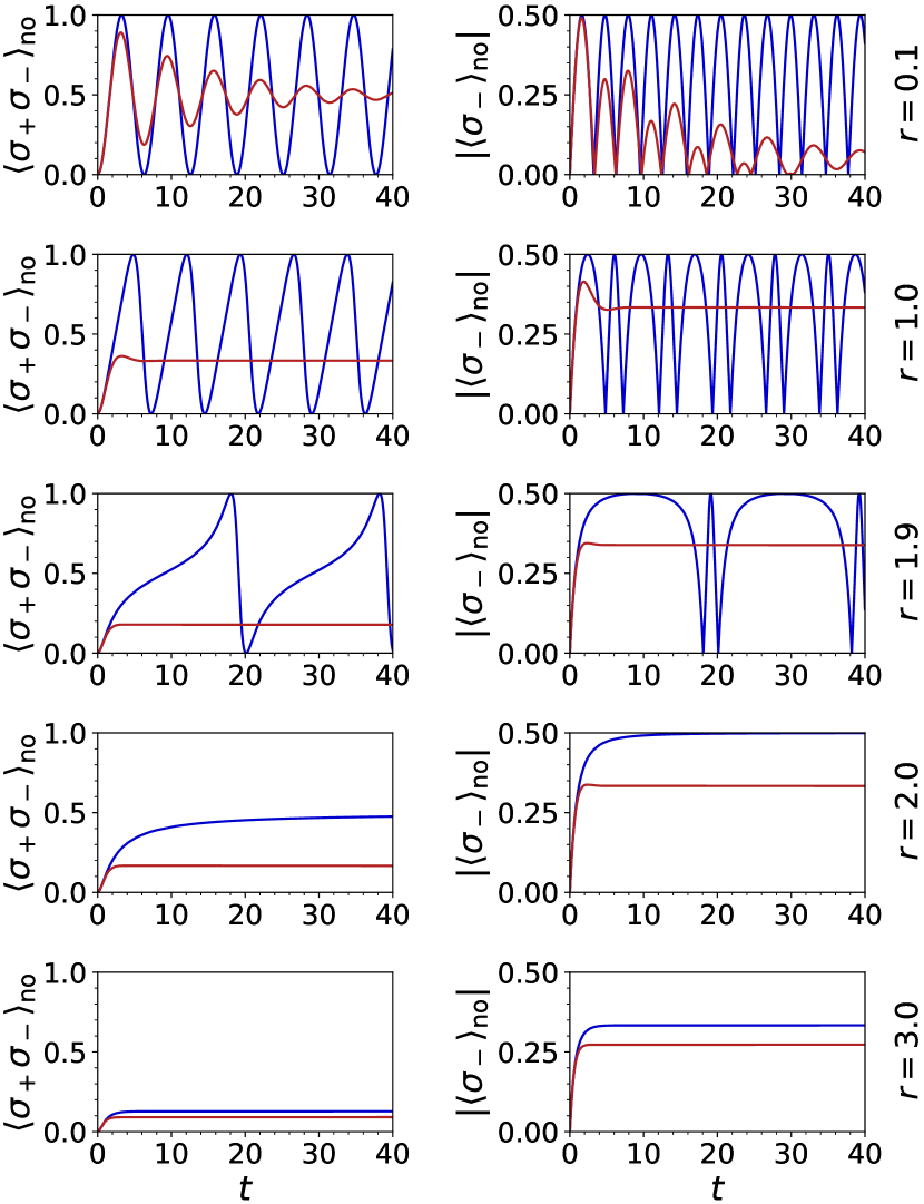
Figure 2: Conditional (Λ=1superscriptΛ1\Lambda^{-}=1; blue) and unconditional (Λ=0superscriptΛ0\Lambda^{-}=0; red) dynamics of a single qubit governed by the master equation (III.1). Left: population q=σ+σno𝑞subscriptdelimited-⟨⟩subscript𝜎subscript𝜎noq=\langle\sigma_{+}\sigma_{-}\rangle_{\rm no}. Right: coherence |c|=|σno|𝑐subscriptdelimited-⟨⟩subscript𝜎no|c|=|\langle\sigma_{-}\rangle_{\rm no}|. Each row is for Ω=1Ω1\Omega=1 and a different value of r=Γ/Ω=0.1,1.0,1.9,2.0,3.0formulae-sequence𝑟ΓΩ0.11.01.92.03.0r=\Gamma/\Omega=0.1,1.0,1.9,2.0,3.0 (from top to bottom).
Refer to caption
Figure 3: (a): Evolution of the no-jump probability Pnosubscript𝑃noP_{\rm no} for Λ=1.0superscriptΛ1.0\Lambda^{-}=1.0, resulting from Fig. 2 (we set Ω=1.0Ω1.0\Omega=1.0 and r=0.1,1.0,1.9,2.0,3.0𝑟0.11.01.92.03.0r=0.1,1.0,1.9,2.0,3.0). (b): Evolution of 1rtlnPno1𝑟𝑡subscript𝑃no-\frac{1}{rt}\ln P_{\rm no} as a function of time t𝑡t, which approaches a finite value for t𝑡t\to\infty. (c) The quantity α(r)/r𝛼𝑟𝑟\alpha(r)/r [Eq. (III.11)], representing the long-time behavior of Pnosubscript𝑃noP_{\rm no}.

The natural operators to consider are the population σ+σsubscript𝜎subscript𝜎\sigma_{+}\sigma_{-} and the coherence σsubscript𝜎\sigma_{-}. We thus define the conditional expectation values q=σ+σno𝑞subscriptdelimited-⟨⟩subscript𝜎subscript𝜎noq=\langle\sigma_{+}\sigma_{-}\rangle_{\rm no} and c=σno𝑐subscriptdelimited-⟨⟩subscript𝜎noc=\langle\sigma_{-}\rangle_{\rm no}. Eq. (II) then yields a system of two coupled non-linear equations

dqdt𝑑𝑞𝑑𝑡\displaystyle\frac{dq}{dt} =iΩ2(cc)Γq+ΓΛq2,absent𝑖Ω2𝑐superscript𝑐Γ𝑞ΓsuperscriptΛsuperscript𝑞2\displaystyle=\frac{i\Omega}{2}(c-c^{*})-\Gamma q+\Gamma\Lambda^{-}q^{2}, (III.2)
dcdt𝑑𝑐𝑑𝑡\displaystyle\frac{dc}{dt} =iΩ2(2q1)Γ2c+ΓΛcq.absent𝑖Ω22𝑞1Γ2𝑐ΓsuperscriptΛ𝑐𝑞\displaystyle=\frac{i\Omega}{2}(2q-1)-\frac{\Gamma}{2}c+\Gamma\Lambda^{-}cq. (III.3)

Once we have their solution, we immediately obtain the no-jump probability (II.19) with

β(t)=ΛΓq(t).𝛽𝑡superscriptΛΓ𝑞𝑡\beta(t)=\Lambda^{-}\Gamma q(t). (III.4)

We prepare the system in the state |zsubscriptket𝑧\ket{\downarrow}_{z} (corresponding to σz|z=|zsubscript𝜎𝑧subscriptket𝑧subscriptket𝑧\sigma_{z}\ket{\downarrow}_{z}=-\ket{\downarrow}_{z}). The parameters (Ω,Γ)ΩΓ(\Omega,\Gamma) affect the no-jump dynamics in a non-trivial way, but Eqs. (III.2), (III.3) clearly show that the steady-state is uniquely determined by the rate r=Γ/Ω>0𝑟ΓΩ0r=\Gamma/\Omega>0, if it exists.

Fig. 2 shows the evolution of q(t)𝑞𝑡q(t) (left) and |c(t)|𝑐𝑡|c(t)| (right) as a function of time for Ω=1Ω1\Omega=1 and different values of the rate r𝑟r. The unconditional dynamics (Λ=0superscriptΛ0\Lambda^{-}=0; no monitoring) shows the typical behavior of a damped oscillator and always relaxes to a steady-state,

qΛ=0=12+r2,|cΛ=0|=rqΛ=0.formulae-sequencesubscriptsuperscript𝑞superscriptΛ012superscript𝑟2subscriptsuperscript𝑐superscriptΛ0𝑟subscriptsuperscript𝑞superscriptΛ0q^{\infty}_{\Lambda^{-}=0}=\frac{1}{2+r^{2}},\qquad\absolutevalue{c^{\infty}_{\Lambda^{-}=0}}=rq^{\infty}_{\Lambda^{-}=0}. (III.5)

The general conditional case Λ(0,1)superscriptΛ01\Lambda^{-}\in(0,1) is more difficult but still shares the same features with the case Λ=0superscriptΛ0\Lambda^{-}=0. The oscillations are damped and qΛsubscriptsuperscript𝑞superscriptΛq^{\infty}_{\Lambda^{-}} is the real positive solution of the cubic equation

2r2(Λ)2(qΛ)33Λr2(qΛ)2+(r2+2)qΛ1=0,2superscript𝑟2superscriptsuperscriptΛ2superscriptsubscriptsuperscript𝑞superscriptΛ33superscriptΛsuperscript𝑟2superscriptsubscriptsuperscript𝑞superscriptΛ2superscript𝑟22subscriptsuperscript𝑞superscriptΛ102r^{2}(\Lambda^{-})^{2}(q^{\infty}_{\Lambda^{-}})^{3}-3\Lambda^{-}r^{2}(q^{\infty}_{\Lambda^{-}})^{2}+(r^{2}+2)q^{\infty}_{\Lambda^{-}}-1=0, (III.6)

with

|cΛ|=rqΛ(1ΛqΛ).subscriptsuperscript𝑐superscriptΛ𝑟subscriptsuperscript𝑞superscriptΛ1superscriptΛsubscriptsuperscript𝑞superscriptΛ\absolutevalue{c^{\infty}_{\Lambda^{-}}}=rq^{\infty}_{\Lambda^{-}}(1-\Lambda^{-}q^{\infty}_{\Lambda^{-}}). (III.7)

Conversely, the full monitoring case (Λ=1superscriptΛ1\Lambda^{-}=1) provides new physical insights. We can identify a critical rate rc=2subscript𝑟𝑐2r_{c}=2 which distinguishes two different regimes. If r<rc𝑟subscript𝑟𝑐r<r_{c}, q(t)𝑞𝑡q(t) and |c(t)|𝑐𝑡|c(t)| are periodic functions and show an oscillatory phase; if rrc𝑟subscript𝑟𝑐r\geq r_{c}, the oscillations are suppressed with an emerging asymptotic state,

qΛ=1subscriptsuperscript𝑞superscriptΛ1\displaystyle q^{\infty}_{\Lambda^{-}=1} =121214r2,absent121214superscript𝑟2\displaystyle=\frac{1}{2}-\frac{1}{2}\sqrt{1-\frac{4}{r^{2}}}, (III.8)
|cΛ=1|subscriptsuperscript𝑐superscriptΛ1\displaystyle\absolutevalue{c^{\infty}_{\Lambda^{-}=1}} =rqΛ=1(1qΛ=1).absent𝑟subscriptsuperscript𝑞superscriptΛ11subscriptsuperscript𝑞superscriptΛ1\displaystyle=rq^{\infty}_{\Lambda^{-}=1}(1-q^{\infty}_{\Lambda^{-}=1}). (III.9)

The insight is that this transition is associated to the spectrum of the non-Hermitian Hamiltonian (II.7)

He=Ω2σxiΓ2σ+σ=12(iΓΩΩ0).subscript𝐻𝑒Ω2subscript𝜎𝑥𝑖Γ2subscript𝜎subscript𝜎12matrix𝑖ΓΩΩ0H_{e}=\frac{\Omega}{2}\sigma_{x}-i\frac{\Gamma}{2}\sigma_{+}\sigma_{-}=\frac{1}{2}\begin{pmatrix}-i\Gamma&\Omega\\ \Omega&0\end{pmatrix}. (III.10)

The no-jump probability is plotted in Fig. 3 (a) for several values of r𝑟r and Ω=1Ω1\Omega=1, showcasing the differences between the oscillatory phase r<rc=2𝑟subscript𝑟𝑐2r<r_{c}=2 and the damped phase, r>rc𝑟subscript𝑟𝑐r>r_{c}. In the long-time limit the no-jump distribution behaves as

Pnoeα(r)t,α(r)={r/2r<rc,rqΛ=1rrc,formulae-sequencesimilar-tosubscript𝑃nosuperscript𝑒𝛼𝑟𝑡𝛼𝑟cases𝑟2𝑟subscript𝑟𝑐𝑟subscriptsuperscript𝑞Λ1𝑟subscript𝑟𝑐P_{\rm no}\sim e^{-\alpha(r)t},\qquad\alpha(r)=\begin{cases}r/2&r<r_{c},\\[5.69046pt] rq^{\infty}_{\Lambda=1}&r\geq r_{c},\end{cases} (III.11)

as shown in Fig. 3 (b), where we plot (rt)1lnPnosuperscript𝑟𝑡1subscript𝑃no-(rt)^{-1}\ln P_{\rm no} as a function of time t𝑡t. Finally, in Fig. 3 (c) we plot α(r)𝛼𝑟\alpha(r), which showcases the abrupt transition between the oscillatory and non-oscillatory phases.

III.1 Incoherent dynamics with emission and absorption

Next we consider a two-level system with trivial Hamiltonian H=Ω2σz𝐻Ω2subscript𝜎𝑧H=\frac{\Omega}{2}\sigma_{z}, interacting with a fermionic bath. The coupling is described by two jump operators L=Γσsubscript𝐿superscriptΓsubscript𝜎L_{-}=\sqrt{\Gamma^{-}}\sigma_{-} and L+=Γ+σ+subscript𝐿superscriptΓsubscript𝜎L_{+}=\sqrt{\Gamma^{+}}\sigma_{+}. L+subscript𝐿L_{+} and Lsubscript𝐿L_{-} determine, respectively, the emission and the absorption of an excitation. We shall adopt the following parametrization

Γ+=Γf,Γ=Γ(1f),formulae-sequencesuperscriptΓΓ𝑓superscriptΓΓ1𝑓\Gamma^{+}=\Gamma f,\qquad\Gamma^{-}=\Gamma(1-f), (III.12)

where Γ>0Γ0\Gamma>0 is the coupling strength to the reservoir and f=(eΩ/T+1)1[0,1]𝑓superscriptsuperscript𝑒Ω𝑇1101f=(e^{\Omega/T}+1)^{-1}\in[0,1] is the Fermi-Dirac distribution of the reservoir (with T𝑇T being the temperature and kB=1subscript𝑘𝐵1k_{B}=1). We again apply Eq. (II) to 𝒪=σ+σ𝒪subscript𝜎subscript𝜎\mathcal{O}=\sigma_{+}\sigma_{-}. Let ΛsuperscriptΛ\Lambda^{-} and Λ+superscriptΛ\Lambda^{+} be the monitoring efficiencies for emission and absorption, respectively. The qubit population conditioned on no jumps being detected, q=σ+σno𝑞subscriptdelimited-⟨⟩subscript𝜎subscript𝜎noq=\langle\sigma_{+}\sigma_{-}\rangle_{\rm no}, evolves according to the non-linear equation

1Γdqdt=fq+(1f)Λq2fΛ+(1q)2.1Γ𝑑𝑞𝑑𝑡𝑓𝑞1𝑓superscriptΛsuperscript𝑞2𝑓superscriptΛsuperscript1𝑞2\frac{1}{\Gamma}\frac{dq}{dt}=f-q+(1-f)\Lambda^{-}q^{2}-f\Lambda^{+}(1-q)^{2}. (III.13)

The first two terms are the same as in the unconditional dynamics, while the last two are the new contributions from monitoring. Plugging the solution in Eq. (II.19) also yields the no-jump probability in the form (II.19) with

β(t)=Γ(1f)Λq(t)+ΓfΛ+(1q(t)).𝛽𝑡Γ1𝑓superscriptΛ𝑞𝑡Γ𝑓superscriptΛ1𝑞𝑡\beta(t)=\Gamma(1-f)\Lambda^{-}q(t)+\Gamma f\Lambda^{+}(1-q(t)). (III.14)

Solving dqdt=0𝑑𝑞𝑑𝑡0\frac{dq}{dt}=0 we find the stationary solution of Eq. (III.13), which is

q=superscript𝑞absent\displaystyle q^{\infty}= (2fΛ+1)24f(1Λ+)(Λf(Λ+Λ+))2(fΛ+fΛ+Λ)\displaystyle\frac{\sqrt{\left(2f\Lambda^{+}-1\right){}^{2}-4f\left(1-\Lambda^{+}\right)\left(\Lambda^{-}-f(\Lambda^{-}+\Lambda^{+})\right)}}{2\left(f\Lambda^{-}+f\Lambda^{+}-\Lambda^{-}\right)}
+2fΛ+12(fΛ+fΛ+Λ).2𝑓superscriptΛ12𝑓superscriptΛ𝑓superscriptΛsuperscriptΛ\displaystyle+\frac{2f\Lambda^{+}-1}{2\left(f\Lambda^{-}+f\Lambda^{+}-\Lambda^{-}\right)}. (III.15)

The result is independent of ΓΓ\Gamma. The cases Λ+,Λ=0,1formulae-sequencesuperscriptΛsuperscriptΛ01\Lambda^{+},\Lambda^{-}=0,1 behave as follows (see also Fig. 4). If Λ+=Λ=0superscriptΛsuperscriptΛ0\Lambda^{+}=\Lambda^{-}=0 we get the unconditional steady-state q=fsuperscript𝑞𝑓q^{\infty}=f. If we only monitor emissions, but not absorptions (Λ=1superscriptΛ1\Lambda^{-}=1 and Λ+=0superscriptΛ0\Lambda^{+}=0) we get

q={f1ff<1/2,1f>1/2,superscript𝑞cases𝑓1𝑓𝑓121𝑓12q^{\infty}=\begin{cases}\frac{f}{1-f}&f<1/2,\\[5.69046pt] 1&f>1/2\end{cases}, (III.16)

which is the red curve in Fig. 4. The rationale is that, since the evolution is conditioned on no emission events having occurred, it is more likely that an excitation is present, leading to a population qfsuperscript𝑞𝑓q^{\infty}\geqslant f. In the opposite scenario (Λ+=1superscriptΛ1\Lambda^{+}=1 and Λ=0superscriptΛ0\Lambda^{-}=0) we get

q={0f<1/2,2f1ff>1/2,superscript𝑞cases0𝑓122𝑓1𝑓𝑓12q^{\infty}=\begin{cases}0&f<1/2,\\[5.69046pt] \frac{2f-1}{f}&f>1/2,\end{cases} (III.17)

which is the green curve in Fig. 4. Here the observer knows with certainty that no excitations are absorbed, and this leads to a population qfsuperscript𝑞𝑓q^{\infty}\leqslant f, i.e. smaller than in the unconditional case. Finally, if Λ=Λ+=1superscriptΛsuperscriptΛ1\Lambda^{-}=\Lambda^{+}=1, we get a step function (blue curve), which reflects the non-trivial interplay of conditioning on both channels.

Refer to caption
Figure 4: Steady-state population qsuperscript𝑞q^{\infty} of the conditional dynamics (III.13) as a function of the Fermi-Dirac occupation f𝑓f, for different choices of (Λ+,Λ)superscriptΛsuperscriptΛ(\Lambda^{+},\Lambda^{-}).

IV No-jump dynamics of non-interacting particles

The previous examples show that even for a single qubit the conditional no-jump dynamics is quite involved. In order to provide further analytical insights, we now specialize to the case of many-body one dimensional systems with Gaussian-preserving dynamics.

More specifically, we consider a chain with L𝐿L sites, each described by an annihilation operator cisubscript𝑐𝑖c_{i}, either bosonic or fermionic,

{ci,cj}subscript𝑐𝑖superscriptsubscript𝑐𝑗\displaystyle\{c_{i},c_{j}^{\dagger}\} =δij,{ci,cj}=0,fermionsformulae-sequenceabsentsubscript𝛿𝑖𝑗subscript𝑐𝑖subscript𝑐𝑗0fermions\displaystyle=\delta_{ij},\quad\{c_{i},c_{j}\}=0,\qquad\text{fermions} (IV.1)
[ci,cj]commutatorsubscript𝑐𝑖subscriptsuperscript𝑐𝑗\displaystyle\commutator{c_{i}}{c^{\dagger}_{j}} =δij,[ci,cj]=0.bosons\displaystyle=\delta_{ij},\quad\commutator{c_{i}}{c_{j}}=0.\qquad\quad\text{bosons} (IV.2)

The system is subject to the Lindblad master equation (II.1) with dissipator of the form

𝒟(ρ)=i=1L(ΓiDρ[Xi]+Γi+Dρ[Xi]).𝒟𝜌superscriptsubscript𝑖1𝐿superscriptsubscriptΓ𝑖subscript𝐷𝜌delimited-[]subscript𝑋𝑖superscriptsubscriptΓ𝑖subscript𝐷𝜌delimited-[]superscriptsubscript𝑋𝑖\mathcal{D}(\rho)=\sum_{i=1}^{L}\left(\Gamma_{i}^{-}D_{\rho}[X_{i}]+\Gamma_{i}^{+}D_{\rho}[X_{i}^{\dagger}]\right). (IV.3)

The dissipator (IV.3) consists of 2L2𝐿2L jump operators {ΓiXi,Γi+Xi}i{1,,L}subscriptsuperscriptΓ𝑖subscript𝑋𝑖subscriptsuperscriptΓ𝑖superscriptsubscript𝑋𝑖for-all𝑖1𝐿\left\{\sqrt{\Gamma^{-}_{i}}X_{i}\,,\,\sqrt{\Gamma^{+}_{i}}X_{i}^{\dagger}\right\}\,\,\forall i\in\{1,\dots,L\} and rates Γi±0superscriptsubscriptΓ𝑖plus-or-minus0\Gamma_{i}^{\pm}\geqslant 0. By hypothesis, the Lindblad operators are linear in the creation/annihilation operators; that is, 𝑿=𝜶𝒄𝑿superscript𝜶𝒄\bm{X}=\bm{\alpha}^{\dagger}\bm{c}, for 𝒄=(c1,,cL)superscript𝒄superscriptsubscript𝑐1superscriptsubscript𝑐𝐿\bm{c}^{\dagger}=(c_{1}^{\dagger},\dots,c_{L}^{\dagger}) and some unitary matrix 𝜶𝜶\bm{\alpha}. The form of the dissipator (IV.3) is thus {IEEEeqnarray}rCl D(ρ) &= ∑_ij=1^L (γ^-)_ij[ c_j ρ c_i^†- 12 {c_i^†c_j, ρ}]
+ ∑_ij=1^L (γ^+)_ij[ c_i^†ρ c_j - 12 {c_j c_i^†, ρ}]. where 𝜸=𝜶𝚪𝜶superscript𝜸𝜶superscript𝚪superscript𝜶\bm{\gamma}^{-}=\bm{\alpha}\bm{\Gamma}^{-}\bm{\alpha}^{\dagger} and 𝜸+=𝜶𝚪+𝜶superscript𝜸𝜶superscript𝚪superscript𝜶\bm{\gamma}^{+}=\bm{\alpha}\bm{\Gamma}^{+}\bm{\alpha}^{\dagger}. Similarly, if Λi+,Λi[0,1]subscriptsuperscriptΛ𝑖subscriptsuperscriptΛ𝑖01\Lambda^{+}_{i},\,\Lambda^{-}_{i}\in[0,1] are the monitoring efficiencies for Xi,Xisuperscriptsubscript𝑋𝑖subscript𝑋𝑖X_{i}^{\dagger},\,X_{i} then the superoperators 0subscript0\mathcal{L}_{0} and 1subscript1\mathcal{L}_{1} read {IEEEeqnarray}rCl L_0(ρ) &= -i [H,ρ] + ∑_ij=1^L [ [γ^-(1-λ^-)]_ij c_j ρ c_i^†- (γ-)ij2 {c_i^†c_j, ρ}]
+ ∑_ij=1^L [ [γ^+(1-λ^+)]_ij c_i^†ρ c_j - (γ+)ij2 {c_j c_i^†, ρ}],

1(ρ)=ij=1L(𝜸𝝀)ijcjρci+ij=1L(𝜸+𝝀+)ijciρcj,subscript1𝜌superscriptsubscript𝑖𝑗1𝐿subscriptsuperscript𝜸superscript𝝀𝑖𝑗subscript𝑐𝑗𝜌superscriptsubscript𝑐𝑖superscriptsubscript𝑖𝑗1𝐿subscriptsuperscript𝜸superscript𝝀𝑖𝑗superscriptsubscript𝑐𝑖𝜌subscript𝑐𝑗\mathcal{L}_{1}({\rho})=\sum\limits_{ij=1}^{L}\left(\bm{\gamma}^{-}\bm{\lambda}^{-}\right)_{ij}{c}_{j}{\rho}{c}_{i}^{\dagger}+\sum\limits_{ij=1}^{L}\left(\bm{\gamma}^{+}\bm{\lambda}^{+}\right)_{ij}{c}_{i}^{\dagger}{\rho}{c}_{j}, (IV.4)

where 𝝀+=𝜶𝚲+𝜶superscript𝝀𝜶superscript𝚲superscript𝜶\bm{\lambda}^{+}=\bm{\alpha}\bm{\Lambda}^{+}\bm{\alpha}^{\dagger}, 𝝀=𝜶𝚲𝜶superscript𝝀𝜶superscript𝚲superscript𝜶\bm{\lambda}^{-}=\bm{\alpha}\bm{\Lambda}^{-}\bm{\alpha}^{\dagger} and H𝐻H is the Hamiltonian of the system. By hypothesis, we assume that H𝐻H is quadratic in the creation and annihilation operators.

The aim of the next sections is to study the no-jump dynamics (IV.3) of non-interacting quantum chains, that means the evolved state ρ~no(t)=e0tρ0subscript~𝜌no𝑡superscript𝑒subscript0𝑡subscript𝜌0{\tilde{\rho}}_{\rm no}(t)=e^{\mathcal{L}_{0}t}\rho_{0} and the normalized state ρno(t)=ρ~no(t)/tr(ρ~no(t))subscript𝜌no𝑡subscript~𝜌no𝑡tracesubscript~𝜌no𝑡{\rho}_{\rm no}(t)={\tilde{\rho}}_{\rm no}(t)/\tr\left({\tilde{\rho}}_{\rm no}(t)\right). The two-point functions cicjno(t)=tr(cicjρno(t))subscriptdelimited-⟨⟩superscriptsubscript𝑐𝑖subscript𝑐𝑗no𝑡tracesuperscriptsubscript𝑐𝑖subscript𝑐𝑗subscript𝜌no𝑡\langle{c}_{i}^{\dagger}{c}_{j}\rangle_{\rm no}(t)=\tr\left({c}_{i}^{\dagger}{c}_{j}{\rho}_{\rm no}(t)\right) give access to the no-jump probability and the WTDs, according to Eqs. (II.17,II.18,II.21,IV.4).

We start studying the simplest case where H=ijhijcicj𝐻subscript𝑖𝑗subscript𝑖𝑗subscriptsuperscript𝑐𝑖subscript𝑐𝑗H=\sum_{ij}h_{ij}c^{\dagger}_{i}c_{j} and then we shall generalize to include pairing terms cicjsubscript𝑐𝑖subscript𝑐𝑗c_{i}c_{j}. As we shall see, the pair creation makes the no-jump dynamics more expensive in terms of computational resources.

V No-jump dynamics without pairing terms - fermionic and bosonic chains

In this section, we shall study the no-jump evolution (IV.3) with the quadratic Hamiltonian

H=𝒄𝒉𝒄,𝒉=𝒉.formulae-sequence𝐻superscript𝒄𝒉𝒄𝒉superscript𝒉H=\bm{c}^{\dagger}\bm{h}\bm{c},\qquad\bm{h}=\bm{h}^{\dagger}. (V.1)

For the moment, we do not include pair creation terms in Eq. (V.1), which will be discussed below, in Sec. VII and Sec. VIII.

V.1 Full monitoring

If each channel is perfectly monitored, 𝚲+=𝚲=𝟙superscript𝚲superscript𝚲1\bm{\Lambda}^{+}=\bm{\Lambda}^{-}=\mathds{1} and the no-jump Liouvillian (IV.3) reduces to

0(ρ)=i[H,ρ]12ij=1L(𝜸𝜸+)ij{cicj,ρ}tr(𝜸+)ρ.subscript0𝜌𝑖𝐻𝜌12superscriptsubscript𝑖𝑗1𝐿subscriptminus-or-plussuperscript𝜸superscript𝜸𝑖𝑗superscriptsubscript𝑐𝑖subscript𝑐𝑗𝜌tracesuperscript𝜸𝜌\mathcal{L}_{0}({\rho})=-i[{H},{\rho}]-\frac{1}{2}\sum_{ij=1}^{L}(\bm{\gamma}^{-}\mp\bm{\gamma}^{+})_{ij}\{{c}_{i}^{\dagger}{c}_{j},{\rho}\}-\tr(\bm{\gamma}^{+}){\rho}. (V.2)

Here the - sign is for fermions and ++ sign for bosons. Since we can study both fermionic and bosonic systems with minimal modifications, hereinafter the sign on top will refer to fermions and the one on bottom to bosons. This convention allows us to write formulas in compact form.

Eq. (V.2) is tantamount to Eq. (II.6) with the non-Hermitian Hamiltonian

He=ij=1L(𝒉e)ijcicjitr(𝜸+)/2,subscript𝐻esuperscriptsubscript𝑖𝑗1𝐿subscriptsubscript𝒉e𝑖𝑗superscriptsubscript𝑐𝑖subscript𝑐𝑗𝑖tracesuperscript𝜸2{H}_{\rm e}=\sum_{ij=1}^{L}(\bm{h}_{\rm e})_{ij}{c}_{i}^{\dagger}{c}_{j}-i\tr(\bm{\gamma}^{+})/2, (V.3)

where

𝒉e=𝒉i2(𝜸𝜸+),subscript𝒉e𝒉𝑖2minus-or-plussuperscript𝜸superscript𝜸\bm{h}_{\rm e}=\bm{h}-\frac{i}{2}(\bm{\gamma}^{-}\mp\bm{\gamma}^{+}), (V.4)

with - sign for fermions and ++ sign for bosons.

V.2 Dynamics under partial monitoring

Here we shall focus on the most general case, where all channels are not perfectly monitored 𝝀+,𝝀𝟙superscript𝝀superscript𝝀1\bm{\lambda}^{+},\bm{\lambda}^{-}\neq\mathds{1} and the no-jump Liouvillian takes the form (IV.3). Differently from the full monitoring case, in order to solve the dynamics, we need additional hypotheses on the initial states.

The evolution generated by the Lindbladian (II.1) with the Hamiltonian (V.1) and the dissipator (IV.3) is Gaussian preserving. Assuming the initial state ρ0subscript𝜌0\rho_{0} is Gaussian, the density operator at time t𝑡t is

ρ(t):=et(ρ0)=e𝒄𝑴t𝒄Zt,assign𝜌𝑡superscript𝑒𝑡subscript𝜌0superscript𝑒superscript𝒄subscript𝑴𝑡𝒄subscript𝑍𝑡{\rho}(t):=e^{\mathcal{L}t}({\rho}_{0})=\frac{e^{-{\bm{c}}^{\dagger}\cdot{\bm{M}}_{t}\cdot\bm{c}}}{Z_{t}}, (V.5)

where

Ztsubscript𝑍𝑡\displaystyle Z_{t} =tr(e𝒄𝑴t𝒄)=[det(𝟙±e𝑴t)]±1,absenttracesuperscript𝑒superscript𝒄subscript𝑴𝑡𝒄superscriptdelimited-[]detplus-or-minus1superscript𝑒subscript𝑴𝑡plus-or-minus1\displaystyle=\tr(e^{-{\bm{c}}^{\dagger}\cdot{\bm{M}}_{t}\cdot\bm{c}})=\left[{\rm det}\left(\mathds{1}\pm e^{-\bm{M}_{t}}\right)\right]^{\pm 1}, (V.6)
𝑴tsubscript𝑴𝑡\displaystyle\bm{M}_{t} =ln(𝟙𝑪𝑪missing),absentminus-or-plus1𝑪𝑪missing\displaystyle=\ln\bigg(\frac{\mathds{1}\mp\bm{C}}{\bm{C}}\bigg{missing}), (V.7)

and

𝑪(t)ij=tr{cjciρ(t)}=cjci(t),𝑪subscript𝑡𝑖𝑗tracesuperscriptsubscript𝑐𝑗subscript𝑐𝑖𝜌𝑡delimited-⟨⟩superscriptsubscript𝑐𝑗subscript𝑐𝑖𝑡\bm{C}(t)_{ij}=\tr\{{c}_{j}^{\dagger}{c}_{i}\leavevmode\nobreak\ {\rho}(t)\Big{\}}=\langle{c_{j}}^{\dagger}{c}_{i}\rangle(t), (V.8)

is the correlation matrix. The matrix 𝑪(t)𝑪𝑡\bm{C}(t) must satisfy specific Lyapunov equation for unconditional dynamics turkeshi2021diffusion; coppola2023wigner

d𝑪dt=(𝑾𝑪+𝑪𝑾)+𝜸+,𝑑𝑪𝑑𝑡𝑾𝑪𝑪superscript𝑾superscript𝜸\frac{d\bm{C}}{dt}=-(\bm{WC}+\bm{CW}^{\dagger})+\bm{\gamma}^{+}, (V.9)

with

𝑾=i𝒉+(𝜸±𝜸+)/2.𝑾𝑖𝒉plus-or-minussuperscript𝜸superscript𝜸2\bm{W}=i\bm{h}+(\bm{\gamma}^{-}\pm\bm{\gamma}^{+})/2. (V.10)

However, the goal is to solve the more general non trace-preserving dynamics (IV.3). Here we shall demonstrate that, if the system is propperly prepared in a Gaussian state at time t=0𝑡0t=0, the dynamics (IV.3) is solved by the Gaussian ansatz

ρ~no(t):=e0t(ρ0)=e𝒄𝑴tno𝒄ζt,assignsubscript~𝜌no𝑡superscript𝑒subscript0𝑡subscript𝜌0superscript𝑒superscript𝒄superscriptsubscript𝑴𝑡no𝒄subscript𝜁𝑡{\tilde{\rho}}_{\rm no}(t):=e^{\mathcal{L}_{0}t}({\rho}_{0})=\frac{e^{-{\bm{c}}^{\dagger}\cdot{\bm{M}}_{t}^{\rm no}\cdot\bm{c}}}{\zeta_{t}}, (V.11)

for some time-dependent matrix 𝑴tnosuperscriptsubscript𝑴𝑡no\bm{M}_{t}^{\rm no} and c𝑐c-number ζtsubscript𝜁𝑡\zeta_{t}, which must satisfy specific differential equations, to be determined. The properly normalized state is then

ρno(t)::subscript𝜌no𝑡absent\displaystyle{\rho}_{\rm no}(t): =ρ~no(t)Pno(t)=e𝒄𝑴tno𝒄Ztno,absentsubscript~𝜌no𝑡subscript𝑃no𝑡superscript𝑒superscript𝒄superscriptsubscript𝑴𝑡no𝒄superscriptsubscript𝑍𝑡no\displaystyle=\frac{{\tilde{\rho}}_{\rm no}(t)}{P_{\rm no}(t)}=\frac{e^{-{\bm{c}}^{\dagger}\cdot{\bm{M}}_{t}^{\rm no}\cdot\bm{c}}}{Z_{t}^{\rm no}}, (V.12)
Ztnosuperscriptsubscript𝑍𝑡no\displaystyle Z_{t}^{\rm no} =tr(e𝒄𝑴tno𝒄)=[det(𝟙±e𝑴tno)]±1.absenttracesuperscript𝑒superscript𝒄superscriptsubscript𝑴𝑡no𝒄superscriptdelimited-[]detplus-or-minus1superscript𝑒superscriptsubscript𝑴𝑡noplus-or-minus1\displaystyle=\tr(e^{-{\bm{c}}^{\dagger}\cdot{\bm{M}}_{t}^{\rm no}\cdot\bm{c}})=\left[{\rm det}\left(\mathds{1}\pm e^{-\bm{M}_{t}^{\rm no}}\right)\right]^{\pm 1}. (V.13)

The two-point functions

𝑪no(t)ijsubscript𝑪nosubscript𝑡𝑖𝑗\displaystyle\bm{C}_{\rm no}(t)_{ij} =tr{cjciρno(t)}=cjcino(t),absenttracesuperscriptsubscript𝑐𝑗subscript𝑐𝑖subscript𝜌no𝑡subscriptdelimited-⟨⟩superscriptsubscript𝑐𝑗subscript𝑐𝑖no𝑡\displaystyle=\tr\{{c}_{j}^{\dagger}{c}_{i}\leavevmode\nobreak\ {\rho}_{\rm no}(t)\Big{\}}=\langle c_{j}^{\dagger}{c}_{i}\rangle_{{\rm no}}(t), (V.14)
=[(e𝑴tno±𝟙)1]ij.absentsubscriptdelimited-[]superscriptplus-or-minussuperscript𝑒superscriptsubscript𝑴𝑡no11𝑖𝑗\displaystyle=[(e^{\bm{M}_{t}^{\rm no}}\pm\mathds{1})^{-1}]_{ij}. (V.15)

fully characterize the Gaussian state ρno(t)subscript𝜌no𝑡{\rho}_{\rm no}(t). In Appendix A, we show that the ansatz (V.11) solves the dynamical map (IV.3). In particular, we derive two independent differential equations for ζtsubscript𝜁𝑡\zeta_{t} and the conditional covariance matrix 𝑪no(t)subscript𝑪no𝑡\bm{C}_{\rm no}(t),

d𝑪nodt=𝑑subscript𝑪no𝑑𝑡absent\displaystyle\frac{d\bm{C}_{\rm no}}{dt}= (𝑾𝑪no+𝑪no𝑾)+𝜸+±𝑪no(𝜸𝝀)𝑪noplus-or-minus𝑾subscript𝑪nosubscript𝑪nosuperscript𝑾superscript𝜸subscript𝑪nosuperscript𝜸superscript𝝀subscript𝑪no\displaystyle-(\bm{W}\bm{C}_{\rm no}+\bm{C}_{\rm no}\bm{W}^{\dagger})+\bm{\gamma}^{+}\pm\bm{C}_{\rm no}(\bm{\gamma}^{-}\bm{\lambda}^{-})\bm{C}_{\rm no}
(𝟙𝑪no)(𝜸+𝝀+)(𝟙𝑪no),minus-or-plus1subscript𝑪nosuperscript𝜸superscript𝝀minus-or-plus1subscript𝑪no\displaystyle-(\mathds{1}\mp\bm{C}_{\rm no})(\bm{\gamma}^{+}\bm{\lambda}^{+})(\mathds{1}\mp\bm{C}_{\rm no}), (V.16)
ddtln(ζ)t=𝑑𝑑𝑡subscript𝜁𝑡absent\displaystyle\frac{d}{dt}\ln{\zeta}_{t}= tr{𝜸+𝜸(𝟙𝝀)𝑪no(t)𝟙𝑪no(t)},tracesuperscript𝜸superscript𝜸1superscript𝝀subscript𝑪no𝑡minus-or-plus1subscript𝑪no𝑡\displaystyle\tr\left\{\bm{\gamma}^{+}-\bm{\gamma}^{-}(\mathds{1}-\bm{\lambda}^{-})\frac{\bm{C}_{\rm no}(t)}{\mathds{1}\mp\bm{C}_{\rm no}(t)}\right\}, (V.17)

where 𝑾𝑾\bm{W} is the matrix into Eq. (V.10). Eq. (V.2) is a Riccati-type differential equation and represents one of the most important results of this work. The solution of Eq. (V.2) provides the conditional evolution under partial monitoring. If there is no monitoring, 𝚲+=𝚲=0superscript𝚲superscript𝚲0\bm{\Lambda}^{+}=\bm{\Lambda}^{-}=0, 𝑪no=𝑪subscript𝑪no𝑪\bm{C}_{\rm no}=\bm{C} and we recover the Lyapunov equation (V.9) for the unconditional dynamics. Conversely, monitoring introduces two extra terms. These are non-linear and individually positive semi-definite. In the language of quantum optics, they are called ’information matrices’, as they establish how our knowledge about the state of the system changes given the information that no jump occurred Genoni2016; Belenchia2022. If 𝚲+=𝚲=𝟙superscript𝚲superscript𝚲1\bm{\Lambda}^{+}=\bm{\Lambda}^{-}=\mathds{1}, the result can also be written more compactly as

d𝑪nodt=(𝑲𝑪no+𝑪no𝑲)𝑪no(𝜸+𝜸)𝑪no,𝑑subscript𝑪no𝑑𝑡𝑲subscript𝑪nosubscript𝑪nosuperscript𝑲subscript𝑪nominus-or-plussuperscript𝜸superscript𝜸subscript𝑪no\frac{d\bm{C}_{\rm no}}{dt}=-(\bm{K}\bm{C}_{\rm no}+\bm{C}_{\rm no}\bm{K}^{\dagger})-\bm{C}_{\rm no}(\bm{\gamma}^{+}\mp\bm{\gamma}^{-})\bm{C}_{\rm no}, (V.18)

where 𝑲=𝑾𝜸+=i𝒉+(𝜸𝜸+)/2𝑲minus-or-plus𝑾superscript𝜸𝑖𝒉minus-or-plussuperscript𝜸superscript𝜸2\bm{K}=\bm{W}\mp\bm{\gamma}^{+}=i\bm{h}+(\bm{\gamma}^{-}\mp\bm{\gamma}^{+})/2.

The evolution of the no-jump probability Pno(t)subscript𝑃no𝑡P_{\rm no}(t) is given by Eq. (II.19), where β(t)𝛽𝑡\beta(t) is specified by Eqs. (II.18,IV.4),

β(t)=tr[𝜸+𝝀+(𝟙𝑪no(t))+𝜸𝝀𝑪no(t)].𝛽𝑡tracesuperscript𝜸superscript𝝀minus-or-plus1subscript𝑪no𝑡superscript𝜸superscript𝝀subscript𝑪no𝑡\beta(t)=\tr[\bm{\gamma}^{+}\bm{\lambda}^{+}(\mathds{1}\mp\bm{C}_{\rm no}(t))+\bm{\gamma}^{-}\bm{\lambda}^{-}\bm{C}_{\rm no}(t)\Big{]}. (V.19)

At long time

β(t)tttr{𝜸+𝝀+(𝟙𝑪no)+𝜸𝝀𝑪no},superscriptsimilar-to-or-equalssimilar-to𝑡𝛽𝑡𝑡tracesuperscript𝜸superscript𝝀minus-or-plus1superscriptsubscript𝑪nosuperscript𝜸superscript𝝀superscriptsubscript𝑪no\beta(t)\stackrel{{\scriptstyle t\sim\infty}}{{\simeq}}t\leavevmode\nobreak\ \tr\{\bm{\gamma}^{+}\bm{\lambda}^{+}(\mathds{1}\mp\bm{C}_{\rm no}^{\infty})+\bm{\gamma}^{-}\bm{\lambda}^{-}\bm{C}_{\rm no}^{\infty}\Big{\}}, (V.20)

where 𝑪nosuperscriptsubscript𝑪no\bm{C}_{\rm no}^{\infty} is the stationary solution of Eq. (V.2). Whence, it follows that Pnosubscript𝑃noP_{\rm no} goes exponentially to 00 for large times.

The no-jump probability Pno(t)subscript𝑃no𝑡P_{\rm no}(t) therefore depends on the entire history of the conditional covariance matrix 𝑪nosubscript𝑪no\bm{C}_{\rm no}, weighed by the emission monitoring rates 𝜸𝝀superscript𝜸superscript𝝀\bm{\gamma}^{-}\bm{\lambda}^{-}, plus the entire history of the matrix (𝟙𝑪no)minus-or-plus1subscript𝑪no(\mathds{1}\mp\bm{C}_{\rm no}) weighed by the absorption monitoring rates 𝜸+𝝀+superscript𝜸superscript𝝀\bm{\gamma}^{+}\bm{\lambda}^{+}. For fermion chains with 𝜸+𝝀+=𝜸𝝀superscript𝜸superscript𝝀superscript𝜸superscript𝝀\bm{\gamma}^{+}\bm{\lambda}^{+}=\bm{\gamma}^{-}\bm{\lambda}^{-}, it is possible to talk about a universal behavior since the no-jump probability Pno(t)subscript𝑃no𝑡P_{\rm no}(t) does not depend on the initial state ρ0subscript𝜌0\rho_{0} or the Hamiltonian (V.1). The insight is that the no-jump probability is not sensitive to the kind of detected quantum jump, whether fermions are absorbed or lost. As an example, we could consider standard one-body gain-loss processes, i.e. 𝜸+𝝀+superscript𝜸superscript𝝀\bm{\gamma}^{+}\bm{\lambda}^{+} and 𝜸𝝀superscript𝜸superscript𝝀\bm{\gamma}^{-}\bm{\lambda}^{-} are diagonal. In such a scenario, the probability of absorbing a fermion on site j𝑗j at time t𝑡t is given by dt(𝜸+𝝀+)j(1cjcjno)𝑑𝑡subscriptsuperscript𝜸superscript𝝀𝑗1subscriptdelimited-⟨⟩subscriptsuperscript𝑐𝑗subscript𝑐𝑗nodt\,(\bm{\gamma}^{+}\bm{\lambda}^{+})_{j}\,(1-\langle c^{\dagger}_{j}c_{j}\rangle_{\rm no}), where dt(𝜸+𝝀+)j𝑑𝑡subscriptsuperscript𝜸superscript𝝀𝑗dt\,(\bm{\gamma}^{+}\bm{\lambda}^{+})_{j} is the probability of selecting the absorption channel j𝑗j and 1cjcjno1subscriptdelimited-⟨⟩subscriptsuperscript𝑐𝑗subscript𝑐𝑗no1-\langle c^{\dagger}_{j}c_{j}\rangle_{\rm no} is the probability that the site j𝑗j is empty; the probability of ejecting a fermion from site j𝑗j at time t𝑡t is given by dt(𝜸𝝀)jcjcjno𝑑𝑡subscriptsuperscript𝜸superscript𝝀𝑗subscriptdelimited-⟨⟩subscriptsuperscript𝑐𝑗subscript𝑐𝑗nodt\,(\bm{\gamma}^{-}\bm{\lambda}^{-})_{j}\,\langle c^{\dagger}_{j}c_{j}\rangle_{\rm no}, where dt(𝜸𝝀)j𝑑𝑡subscriptsuperscript𝜸superscript𝝀𝑗dt\,(\bm{\gamma}^{-}\bm{\lambda}^{-})_{j} is the probability of selecting the dissipative channel j𝑗j and cjcjnosubscriptdelimited-⟨⟩subscriptsuperscript𝑐𝑗subscript𝑐𝑗no\langle c^{\dagger}_{j}c_{j}\rangle_{\rm no} is the probability that the site j𝑗j is filled. Hence, the probability that a quantum jump occurs on site j𝑗j is the sum of the two probabilities. Therefore, when the gain and loss rates coincide, i.e. 𝜸+𝝀+=𝜸𝝀superscript𝜸superscript𝝀superscript𝜸superscript𝝀\bm{\gamma}^{+}\bm{\lambda}^{+}=\bm{\gamma}^{-}\bm{\lambda}^{-}, the probability is independent on the local density.

VI Example: tight-binding model

As an application, we consider a chain of hopping fermions with open boundary conditions (OBC) and Hamiltonian

H=i=1L1(cici+1+ci+1ci),𝐻superscriptsubscript𝑖1𝐿1superscriptsubscript𝑐𝑖subscript𝑐𝑖1superscriptsubscript𝑐𝑖1subscript𝑐𝑖H=-\sum\limits_{i=1}^{L-1}\left(c_{i}^{\dagger}c_{i+1}+c_{i+1}^{\dagger}c_{i}\right), (VI.1)

being a typical example of ballistic transport. To illustrate the interesting physics that may emerge, we consider the following non-standard configuration for the reservoirs. The first site is assumed to be coupled to an injection (gain) bath with jump operator c1superscriptsubscript𝑐1c_{1}^{\dagger} and rate Γ1+=ΓsuperscriptsubscriptΓ1Γ\Gamma_{1}^{+}=\Gamma. All other sites are connected to emission (loss) baths with jump operators cisubscript𝑐𝑖c_{i} and rates Γj=ΓsubscriptsuperscriptΓ𝑗Γ\Gamma^{-}_{j}=\Gamma j{2,,L}for-all𝑗2𝐿\forall j\in\{2,\dots,L\}. By hypothesis, we assume perfect monitoring on site 111 (i.e. Λ1+=1superscriptsubscriptΛ11\Lambda_{1}^{+}=1) and a non-ideal monitoring efficiency Λj=ΛsubscriptsuperscriptΛ𝑗superscriptΛ\Lambda^{-}_{j}=\Lambda^{-} j{2,,L}for-all𝑗2𝐿\forall j\in\{2,\dots,L\}. In this view, the no-jump conditional dynamics is given by

0(ρ)=subscript0𝜌absent\displaystyle\mathcal{L}_{0}({\rho})= i[H,ρ]Γ2{c1c1,ρ}𝑖𝐻𝜌Γ2subscript𝑐1superscriptsubscript𝑐1𝜌\displaystyle-i[{H},{\rho}]-\frac{\Gamma}{2}\{c_{1}c_{1}^{\dagger},\rho\}
+Γj=2L((1Λ)cjρcj12{cjcj,ρ}).Γsuperscriptsubscript𝑗2𝐿1superscriptΛsubscript𝑐𝑗𝜌superscriptsubscript𝑐𝑗12superscriptsubscript𝑐𝑗subscript𝑐𝑗𝜌\displaystyle+\Gamma\sum_{j=2}^{L}\left((1-\Lambda^{-}){c}_{j}{\rho}{c}_{j}^{\dagger}-\frac{1}{2}\{c_{j}^{\dagger}c_{j},{\rho}\}\right). (VI.2)

Suppose the system is prepared in the vacuum state |0ket0\ket{0} and undergoes a jump in the channel (1,+)1(1,+) at time t=0𝑡0t=0. ρ(0)=c1|00|c1𝜌0superscriptsubscript𝑐1ket0bra0subscript𝑐1\rho(0)={c}_{1}^{\dagger}\ket{0}\bra{0}c_{1} is still a Gaussian state and represents a paradigmatic example for transport protocols, where a wavepacket is inserted in an empty chain and one studies the propagation. According to the quasi-particle picture, an excitation on site 111 spreads ballistically to the RHS of the chain and is destroyed with rate ΓΓ\Gamma on all the other sites, eventually reaching the second boundary after time L/2𝐿2L/2 coppola2023wigner; castro2016emergent; ruggiero2020quantum; doyon2020lecture; bastianello2019generalized; capizzi2022domain; scopa2022exact; fagotti2017higher; scopa2021exact; dubail2017conformal; collura2018analytic; collura2020domain; alba2021generalized; bouchoule2022generalized; bulchandani2017solvable; bulchandani2018bethe; doyon2018soliton; schemmer2019generalized; malvania2021generalized; collura2012entangling; wendenbaum2013hydrodynamic; cao2019entanglement; jin2021interplay; bouchoule2020effect; dast2014quantum; alba2022noninteracting; alba2022hydrodynamics; carollo2022dissipative. In the meantime, any jump event which occurs on site 111 is automatically detected.

Since Λ1superscriptΛ1\Lambda^{-}\neq 1, not all emission clicks are detected; for this reason, we expect Pnosubscript𝑃noP_{\rm no} to decrease faster for larger efficiencies ΛsuperscriptΛ\Lambda^{-}. The no-jump probability always approaches exponentially 00 for large times. Since we are interested in the thermodynamic limit, we focus on the evolution in the time window [0,L/2]0𝐿2[0,L/2]. In this way, we avoid all the secondary processes due to the finite size effects, with the wavepackets moving back and forth multiple times within the chain.
Refer to caption
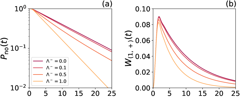
Figure 5: Conditional dynamics for a quantum chain of hopping fermions, Γ=0.1Γ0.1\Gamma=0.1 and several values of the monitoring efficiency Λ={0,0.1,0.5,1.0}superscriptΛ00.10.51.0\Lambda^{-}=\{0,0.1,0.5,1.0\}. (a) no-jump probability Pno(t)subscript𝑃no𝑡P_{\rm no}(t) as a function of time in semi-log scale; (b) waiting-time distribution W(1,+)(t)subscript𝑊1𝑡W_{(1,+)}(t) between two consecutive jumps in the channel (1,+)1(1,+).

In Fig. 5 (a), we plot the no-jump probability Pno(t)subscript𝑃no𝑡P_{\rm no}(t) for Γ=0.1Γ0.1\Gamma=0.1, system size L=50𝐿50L=50 and efficiency Λ={0,0.1,0.5,1.0}superscriptΛ00.10.51.0\Lambda^{-}=\{0,0.1,0.5,1.0\}. At time t=0𝑡0t=0, Pno(t)=1subscript𝑃no𝑡1P_{\rm no}(t)=1 as expected and, at early times, Pno(t)subscript𝑃no𝑡P_{\rm no}(t) is roughly independent of ΛsuperscriptΛ\Lambda^{-}. This phenomenon finds a simple explanation in generalized hydrodynamics. For the specific tight-binding Hamiltonian (VI.1), any particle located on site 111 needs at least Δt=0.5Δ𝑡0.5\Delta t=0.5 to reach the consecutive site and eventually be ejected. According to this rough picture, for t<0.5𝑡0.5t<0.5 the particle cannot be ejected, independently on the monitoring efficiency. At long time, Fig. 5 (a) clearly shows the exponential decay of Pnosubscript𝑃noP_{\rm no}, which is dominated by the parameter ΛsuperscriptΛ\Lambda^{-} and the steady-state 𝑪nosubscriptsuperscript𝑪no\bm{C}^{\infty}_{\rm no}.

In Fig. 5 (b) we plot the waiting-time distribution W(1,+)(t)subscript𝑊1𝑡W_{(1,+)}(t) between two consecutive jumps. In fact, W(1,+)(t)subscript𝑊1𝑡W_{(1,+)}(t) is the conditional probability distribution to observe the second injection on site 111 at time t𝑡t, known that one fermion has been absorbed on site 111 at time t=0𝑡0t=0. From Eq. (II.21), the waiting-time distribution W(1,+)(t)subscript𝑊1𝑡W_{(1,+)}(t) reads

W(1,+)(t)subscript𝑊1𝑡\displaystyle W_{(1,+)}(t) =ΓPno(t)(1𝑪no(t)11),absentΓsubscript𝑃no𝑡1subscript𝑪nosubscript𝑡11\displaystyle=\Gamma P_{\rm no}(t)\left(1-\bm{C}_{\rm no}(t)_{11}\right), (VI.3)

The behavior of W(1,+)(t)subscript𝑊1𝑡W_{(1,+)}(t) clearly reflects the fermionic nature (IV.1). In fact, due to the finite capacity, W(1,+)(t)subscript𝑊1𝑡W_{(1,+)}(t) is null at t=0𝑡0t=0 and then increases. As for the no-jump probability, W(1,+)(t)subscript𝑊1𝑡W_{(1,+)}(t) is also independent on ΛsuperscriptΛ\Lambda^{-} at early times.

Refer to caption
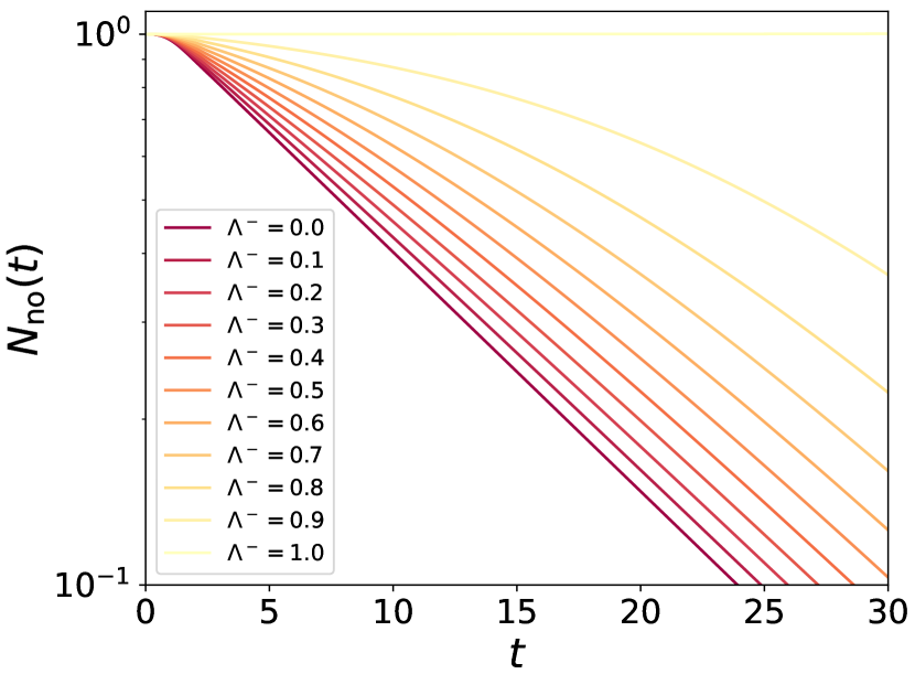
Figure 6: Conditional no-jump evolution of the number of particles Nno(t)=j=1Lcjcjno(t)subscript𝑁no𝑡superscriptsubscript𝑗1𝐿subscriptdelimited-⟨⟩superscriptsubscript𝑐𝑗subscript𝑐𝑗no𝑡N_{\rm no}(t)=\sum_{j=1}^{L}\langle c_{j}^{\dagger}c_{j}\rangle_{\rm no}(t) as a function of time t𝑡t in semi-log scale. Here the time evolution of Nno(t)subscript𝑁no𝑡N_{\rm no}(t) for several monitoring efficiencies Λ=0.1nn{0,,10}superscriptΛ0.1𝑛for-all𝑛010\Lambda^{-}=0.1n\,\,\,\,\forall n\in\{0,\dots,10\}.

In Fig. 6, we show the evolution of Nno(t)=j=1Lcjcjno(t)subscript𝑁no𝑡superscriptsubscript𝑗1𝐿subscriptdelimited-⟨⟩superscriptsubscript𝑐𝑗subscript𝑐𝑗no𝑡N_{\rm no}(t)=\sum_{j=1}^{L}\langle c_{j}^{\dagger}c_{j}\rangle_{\rm no}(t) as a function of time t𝑡t. For Λ=1superscriptΛ1\Lambda^{-}=1, Nno=1subscript𝑁no1N_{\rm no}=1 is a constant of motion because any occurred jump event is automatically detected thanks to the perfect efficiency of the monitoring apparatus. In the opposite case Λ=0superscriptΛ0\Lambda^{-}=0, once the particle leaves the site 111, the statistics of the emission events follows a Poisson distribution, with Nno(t)eΓtsimilar-to-or-equalssubscript𝑁no𝑡superscript𝑒Γ𝑡N_{\rm no}(t)\simeq e^{-\Gamma t} being the probability of finding the particle in the chain at time t𝑡t. In general, Nnosubscript𝑁noN_{\rm no} increases with the efficiency ΛsuperscriptΛ\Lambda^{-}, since for large values of ΛsuperscriptΛ\Lambda^{-} any particle loss is more likely detected. It is interesting to observe that, in the long time limit, Nno(t)eΓtproportional-tosubscript𝑁no𝑡superscript𝑒Γ𝑡N_{\rm no}(t)\propto e^{-\Gamma t} for any efficiency ΛsuperscriptΛ\Lambda^{-}, suggesting that a the monitoring efficiency may affect the dynamics of Nnosubscript𝑁noN_{\rm no} only at finite times.

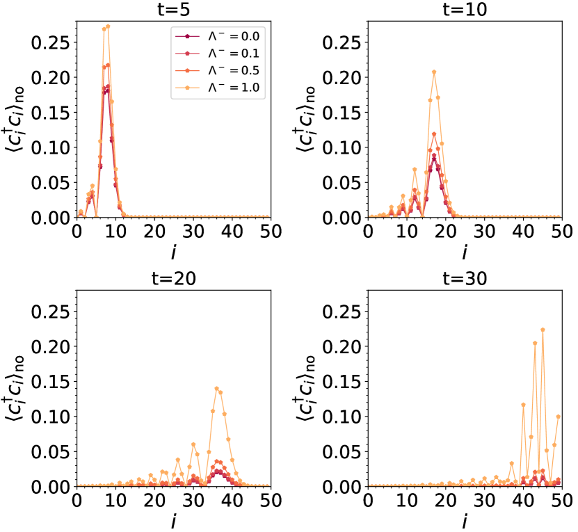
Fig. 7 shows the conditional time evolution of the local occupation cicinosubscriptdelimited-⟨⟩subscriptsuperscript𝑐𝑖subscript𝑐𝑖no\langle c^{\dagger}_{i}c_{i}\rangle_{\rm no}. At time t=0𝑡0t=0, we have c1c1no=1subscriptdelimited-⟨⟩subscriptsuperscript𝑐1subscript𝑐1no1\langle c^{\dagger}_{1}c_{1}\rangle_{\rm no}=1 since we inject a fermion on site 111. After quenching the state, the system evolves with the no-jump operator (VI). As expected, the higher the efficiency ΛsuperscriptΛ\Lambda^{-}, the bigger the local density since the missed detection of loss processes is less likely.
Refer to caption
Figure 7: Time evolution of the local occupation for Γ=0.1Γ0.1\Gamma=0.1 and monitoring efficiency Λ={0,0.1,0.5,1.0}superscriptΛ00.10.51.0\Lambda^{-}=\{0,0.1,0.5,1.0\}. As expected, the larger the efficiency the bigger the fermionic occupation, since any loss event cannot be detected in the time window [0,t]0𝑡[0,t]. Starting from t25similar-to𝑡25t\sim 25, we observe finite size effects and the front wave is reflected according to the open boundary conditions.

VII No-jump dynamics with pairing terms - fermionic chains

We now generalize the dynamics to include pairing terms cicjsubscript𝑐𝑖subscript𝑐𝑗{c}_{i}{c}_{j} in the Hamiltonian operator. For clarity, we prefer to treat the fermionic and bosonic cases in two different sections.

In this section, we shall focus on fermionic chains (IV.1). We introduce the 2L2𝐿2L Majorana operators

yn1=cn+cn,yn2=i(cncn).n=1,,L{y}_{n}^{1}={c}_{n}^{\dagger}+c_{n},\qquad{y}_{n}^{2}=i({c}_{n}^{\dagger}-{c}_{n}).\qquad n=1,\ldots,L (VII.1)

These operators are Hermitian (yk1=yk1superscriptsubscript𝑦𝑘1subscriptsuperscript𝑦1𝑘{y}_{k}^{1\dagger}={y}^{1}_{k}, yk2=yk2superscriptsubscript𝑦𝑘2subscriptsuperscript𝑦2𝑘{y}_{k}^{2\dagger}={y}^{2}_{k}) and satisfy the Clifford algebra

{yk1,y1}=2δk,{yk2,y2}=2δk,{yk1,y2}=0.formulae-sequencesubscriptsuperscript𝑦1𝑘subscriptsuperscript𝑦12subscript𝛿𝑘formulae-sequencesubscriptsuperscript𝑦2𝑘subscriptsuperscript𝑦22subscript𝛿𝑘subscriptsuperscript𝑦1𝑘subscriptsuperscript𝑦20\{{y}^{1}_{k},{y}^{1}_{\ell}\}=2\delta_{k\ell},\qquad\{{y}^{2}_{k},{y}^{2}_{\ell}\}=2\delta_{k\ell},\qquad\{{y}^{1}_{k},{y}^{2}_{\ell}\}=0. (VII.2)

From this it follows that (yk1)2=(yk2)2=𝟙superscriptsuperscriptsubscript𝑦𝑘12superscriptsuperscriptsubscript𝑦𝑘221({y}_{k}^{1})^{2}=({y}_{k}^{2})^{2}={\mathds{1}}. Below, we work with the vector 𝒀=(y11,,yL1,y12,,yL2)superscript𝒀superscriptsubscript𝑦11superscriptsubscript𝑦𝐿1superscriptsubscript𝑦12superscriptsubscript𝑦𝐿2{\bm{Y}}^{\dagger}=({y}_{1}^{1},\ldots,{y}_{L}^{1},{y}_{1}^{2},\ldots,{y}_{L}^{2}), which then satisfies

{Yi,Yj}=2δij,subscript𝑌𝑖subscript𝑌𝑗2subscript𝛿𝑖𝑗\{Y_{i},Y_{j}\}=2\delta_{ij}, (VII.3)

and 𝒀𝒀=2Lsuperscript𝒀𝒀2𝐿{\bm{Y}}^{\dagger}\cdot{\bm{Y}}=2L. The most general quadratic Hamiltonian is

H=14𝒀𝓣𝒀,𝐻14superscript𝒀𝓣𝒀H=\frac{1}{4}{\bm{Y}}^{\dagger}\cdot\bm{\mathcal{T}}\cdot{\bm{Y}}, (VII.4)

where 𝓣𝓣\bm{\mathcal{T}} is a 2L×2L2𝐿2𝐿2L\times 2L Hermitian matrix. In Appendix B we show that, without loss of generality, we can assume 𝓣𝓣\bm{\mathcal{T}} to be anti-symmetric. On the other hand, in Appendix C we prove that the dissipator (IV.3) may be put in the form

𝒟(ρ)=i,j=12LΥij[YiρYj12{YjYi,ρ}],𝒟𝜌superscriptsubscript𝑖𝑗12𝐿subscriptΥ𝑖𝑗delimited-[]subscript𝑌𝑖𝜌subscript𝑌𝑗12subscript𝑌𝑗subscript𝑌𝑖𝜌\mathcal{D}(\rho)=\sum\limits_{i,j=1}^{2L}\Upsilon_{ij}\left[Y_{i}\rho Y_{j}-\frac{1}{2}\{Y_{j}Y_{i},\rho\}\right], (VII.5)

where

𝚼=14(𝜸++(𝜸)Ti[𝜸+(𝜸)T]i[𝜸+(𝜸)T]𝜸++(𝜸)T).𝚼14matrixsuperscript𝜸superscriptsuperscript𝜸T𝑖delimited-[]superscript𝜸superscriptsuperscript𝜸T𝑖delimited-[]superscript𝜸superscriptsuperscript𝜸Tsuperscript𝜸superscriptsuperscript𝜸T\bm{\Upsilon}=\frac{1}{4}\begin{pmatrix}\bm{\gamma}^{+}+(\bm{\gamma}^{-})^{\text{T}}&i\Big{[}\bm{\gamma}^{+}-(\bm{\gamma}^{-})^{\text{T}}\Big{]}\\[5.69046pt] -i\Big{[}\bm{\gamma}^{+}-(\bm{\gamma}^{-})^{\text{T}}\Big{]}&\bm{\gamma}^{+}+(\bm{\gamma}^{-})^{\text{T}}\end{pmatrix}. (VII.6)

The same holds for the no-jump dynamics (IV.3),

0(ρ)=i[H,ρ]+i,j=12L[[𝚼𝚽]ijYiρYj(𝚼)ij2{YjYi,ρ}],subscript0𝜌𝑖𝐻𝜌superscriptsubscript𝑖𝑗12𝐿delimited-[]subscriptdelimited-[]𝚼𝚽𝑖𝑗subscript𝑌𝑖𝜌subscript𝑌𝑗subscript𝚼𝑖𝑗2subscript𝑌𝑗subscript𝑌𝑖𝜌\mathcal{L}_{0}({\rho})=-i[{H},{\rho}]+\sum\limits_{i,j=1}^{2L}\left[[\bm{\Upsilon}-\bm{\Phi}]_{ij}Y_{i}\rho Y_{j}-\frac{(\bm{\Upsilon})_{ij}}{2}\{Y_{j}Y_{i},\rho\}\right], (VII.7)

where

𝚽=14(𝜸+𝝀++(𝜸𝝀)Ti[𝜸+𝝀+(𝜸𝝀)T]i[𝜸+𝝀+(𝜸𝝀)T]𝜸+𝝀++(𝜸𝝀)T).𝚽14matrixsuperscript𝜸superscript𝝀superscriptsuperscript𝜸superscript𝝀T𝑖delimited-[]superscript𝜸superscript𝝀superscriptsuperscript𝜸superscript𝝀T𝑖delimited-[]superscript𝜸superscript𝝀superscriptsuperscript𝜸superscript𝝀Tsuperscript𝜸superscript𝝀superscriptsuperscript𝜸superscript𝝀T\bm{\Phi}=\frac{1}{4}\begin{pmatrix}\bm{\gamma}^{+}\bm{\lambda}^{+}+(\bm{\gamma}^{-}\bm{\lambda}^{-})^{\text{T}}&i\Big{[}\bm{\gamma}^{+}\bm{\lambda}^{+}-(\bm{\gamma}^{-}\bm{\lambda}^{-})^{\text{T}}\Big{]}\\[5.69046pt] -i\Big{[}\bm{\gamma}^{+}\bm{\lambda}^{+}-(\bm{\gamma}^{-}\bm{\lambda}^{-})^{\text{T}}\Big{]}&\bm{\gamma}^{+}\bm{\lambda}^{+}+(\bm{\gamma}^{-}\bm{\lambda}^{-})^{\text{T}}\end{pmatrix}. (VII.8)

Notice that, in general, 𝚼=𝚼superscript𝚼𝚼\bm{\Upsilon}^{\dagger}=\bm{\Upsilon}, 𝚽=𝚽superscript𝚽𝚽\bm{\Phi}^{\dagger}=\bm{\Phi}, but 𝚼T𝚼superscript𝚼T𝚼\bm{\Upsilon}^{\text{T}}\neq\bm{\Upsilon}, 𝚽T𝚽superscript𝚽T𝚽\bm{\Phi}^{\text{T}}\neq\bm{\Phi}.

VII.1 Full monitoring

When all channels are perfectly monitored, 𝚲+=𝚲=𝟙superscript𝚲superscript𝚲1\bm{\Lambda}^{+}=\bm{\Lambda}^{-}=\mathds{1} and 𝚼=𝚽𝚼𝚽\bm{\Upsilon}=\bm{\Phi}. The no-jump operator (VII.7) reduces to

0(ρ)=i[H,ρ]12i,j=12L(𝚼)ij{YjYi,ρ}.subscript0𝜌𝑖𝐻𝜌12superscriptsubscript𝑖𝑗12𝐿subscript𝚼𝑖𝑗subscript𝑌𝑗subscript𝑌𝑖𝜌\mathcal{L}_{0}({\rho})=-i[{H},{\rho}]-\frac{1}{2}\sum\limits_{i,j=1}^{2L}(\bm{\Upsilon})_{ij}\{Y_{j}Y_{i},\rho\}. (VII.9)

After some algebra, 0subscript0\mathcal{L}_{0} takes the form (II.6) with effective Hamiltonian

He=𝒀𝓣+i(𝚼𝚼T)4𝒀itr(𝚼)2.subscript𝐻𝑒superscript𝒀𝓣𝑖𝚼superscript𝚼T4𝒀𝑖trace𝚼2{H}_{e}={\bm{Y}}^{\dagger}\cdot\frac{\bm{\mathcal{T}}+i(\bm{\Upsilon}-\bm{\Upsilon}^{{}^{\text{T}}})}{4}\cdot{\bm{Y}}-i\frac{\tr(\bm{\Upsilon})}{2}. (VII.10)

VII.2 Dynamics under partial monitoring

We now derive the conditional dynamics under partial monitoring, following closely the calculations (and the notation) of Sec. V.2. We assume that the initial state is Gaussian. The unconditional dynamics (II.1) with the Hamiltonian (VII.4), the dissipator (VII.5) and the matrix (VII.6) is Gaussian preserving,

ρ(t):=et(ρ0)=e14𝒀𝓜t𝒀Zt,assign𝜌𝑡superscript𝑒𝑡subscript𝜌0superscript𝑒14superscript𝒀subscript𝓜𝑡𝒀subscript𝑍𝑡{\rho}(t):=e^{\mathcal{L}t}({\rho}_{0})=\frac{e^{\frac{1}{4}{{\bm{Y}}}^{\dagger}\cdot\bm{\mathcal{M}}_{t}\cdot{\bm{Y}}}}{Z_{t}}, (VII.11)

where 𝓜tsubscript𝓜𝑡\bm{\mathcal{M}}_{t} is Hermitian and anti-symmetric,

Ztsubscript𝑍𝑡\displaystyle Z_{t} =tr{e14𝒀𝓜t𝒀}=det(𝟙+e𝓜t),absenttracesuperscript𝑒14superscript𝒀subscript𝓜𝑡𝒀1superscript𝑒subscript𝓜𝑡\displaystyle=\tr\{e^{\frac{1}{4}{{\bm{Y}}}^{\dagger}\cdot\bm{\mathcal{M}}_{t}\cdot{\bm{Y}}}\Big{\}}=\sqrt{\det(\mathds{1}+e^{\bm{\mathcal{M}}_{t}})}, (VII.12)
𝓜tsubscript𝓜𝑡\displaystyle\bm{\mathcal{M}}_{t} =ln(𝟙𝚯𝟙+𝚯missing),absent1𝚯1𝚯missing\displaystyle=\ln\bigg(\frac{\mathds{1}-\bm{\Theta}}{\mathds{1}+\bm{\Theta}}\bigg{missing}), (VII.13)

and

𝚯(t)ij=12tr{[Yi,Yj]ρ(t)}=12[Yi,Yj](t),𝚯subscript𝑡𝑖𝑗12tracesubscript𝑌𝑖subscript𝑌𝑗𝜌𝑡12delimited-⟨⟩subscript𝑌𝑖subscript𝑌𝑗𝑡\bm{\Theta}(t)_{ij}=\frac{1}{2}\tr\{[Y_{i},Y_{j}]\rho(t)\Big{\}}=\frac{1}{2}\langle[Y_{i},Y_{j}]\rangle(t), (VII.14)

is the correlation matrix, which is Hermitian (𝚯=𝚯superscript𝚯𝚯\bm{\Theta}^{\dagger}=\bm{\Theta}) and anti-symmetric (𝚯T=𝚯superscript𝚯T𝚯\bm{\Theta}^{\text{T}}=-\bm{\Theta}) as well. The correlation matrix 𝚯𝚯\bm{\Theta} satisfies the Lyapunov differential equation Purkayastha2022

d𝚯dt=(𝓦𝚯+𝚯𝓦)+𝓕,𝑑𝚯𝑑𝑡𝓦𝚯𝚯superscript𝓦𝓕\frac{d\bm{\Theta}}{dt}=-\big{(}\bm{\mathcal{W}}\bm{\Theta}+\bm{\Theta}\bm{\mathcal{W}}^{\dagger}\big{)}+\bm{\mathcal{F}}, (VII.15)

with

𝓦𝓦\displaystyle\bm{\mathcal{W}} =i𝓣+𝚼+𝚼T,absent𝑖𝓣𝚼superscript𝚼T\displaystyle=i\bm{\mathcal{T}}+\bm{\Upsilon}+\bm{\Upsilon}^{\text{T}}, (VII.16)
𝓕𝓕\displaystyle\bm{\mathcal{F}} =2(𝚼T𝚼).absent2superscript𝚼T𝚼\displaystyle=2(\bm{\Upsilon}^{\text{T}}-\bm{\Upsilon}). (VII.17)

Here we show that the conditional no-jump dynamics (VII.7) is solved by the Gaussian ansatz

ρ~no(t):=e0t(ρ0)=e14𝒀𝓜tno𝒀ζt,assignsubscript~𝜌no𝑡superscript𝑒subscript0𝑡subscript𝜌0superscript𝑒14superscript𝒀superscriptsubscript𝓜𝑡no𝒀subscript𝜁𝑡{\tilde{\rho}}_{\rm no}(t):=e^{\mathcal{L}_{0}t}({\rho}_{0})=\frac{e^{\frac{1}{4}{{\bm{Y}}}^{\dagger}\cdot\bm{\mathcal{M}}_{t}^{\rm no}\cdot{\bm{Y}}}}{\zeta_{t}}, (VII.18)

for some time-dependent matrix 𝓜tnosuperscriptsubscript𝓜𝑡no\bm{\mathcal{M}}_{t}^{\rm no} and c𝑐c-number ζtsubscript𝜁𝑡\zeta_{t}, which must satisfy specific differential equations, to be determined. Again, the properly normalized state is

ρno(t)subscript𝜌no𝑡\displaystyle{\rho}_{\rm no}(t) :=ρ~no(t)Pno(t)=e14𝒀𝓜tno𝒀Ztno,assignabsentsubscript~𝜌no𝑡subscript𝑃no𝑡superscript𝑒14superscript𝒀superscriptsubscript𝓜𝑡no𝒀superscriptsubscript𝑍𝑡no\displaystyle:=\frac{{\tilde{\rho}}_{\rm no}(t)}{P_{\rm no}(t)}=\frac{e^{\frac{1}{4}{{\bm{Y}}}^{\dagger}\cdot\bm{\mathcal{M}}_{t}^{\rm no}\cdot{\bm{Y}}}}{Z_{t}^{\rm no}}, (VII.19)
Ztnosuperscriptsubscript𝑍𝑡no\displaystyle Z_{t}^{\rm no} =tr{e14𝒀𝓜tno𝒀}=det(𝟙+e𝓜tno).absenttracesuperscript𝑒14superscript𝒀superscriptsubscript𝓜𝑡no𝒀1superscript𝑒subscriptsuperscript𝓜no𝑡\displaystyle=\tr\{e^{\frac{1}{4}{{\bm{Y}}}^{\dagger}\cdot\bm{\mathcal{M}}_{t}^{\rm no}\cdot{\bm{Y}}}\Big{\}}=\sqrt{\det(\mathds{1}+e^{\bm{\mathcal{M}}^{\rm no}_{t}})}. (VII.20)

The correlation matrix

𝚯no(t)ijsubscript𝚯nosubscript𝑡𝑖𝑗\displaystyle\bm{\Theta}_{\rm no}(t)_{ij} =[tanh(𝓜tno/2)]ij=12[Yi,Yj]no(t),absentsubscriptdelimited-[]superscriptsubscript𝓜𝑡no2𝑖𝑗12subscriptdelimited-⟨⟩subscript𝑌𝑖subscript𝑌𝑗no𝑡\displaystyle=-[\tanh(\bm{\mathcal{M}}_{t}^{\rm no}/2)]_{ij}=\frac{1}{2}\langle[Y_{i},Y_{j}]\rangle_{\rm no}(t), (VII.21)

fully characterizes the state ρno(t)subscript𝜌no𝑡{\rho}_{\rm no}(t). The matrix 𝚯nosubscript𝚯no\bm{\Theta}_{\rm no} can also be put in the block form

𝚯no=(𝚯1,noi𝚯3,noi𝚯3,no𝚯2,no),subscript𝚯nomatrixsubscript𝚯1no𝑖subscript𝚯3no𝑖superscriptsubscript𝚯3nosubscript𝚯2no\displaystyle\bm{\Theta}_{\rm no}=\begin{pmatrix}\bm{\Theta}_{1,\rm no}&-i\bm{\Theta}_{3,\rm no}\\[5.69046pt] i\bm{\Theta}_{3,\rm no}^{\dagger}&\bm{\Theta}_{2,\rm no}\end{pmatrix}, (VII.22)

where

𝚯1,nosubscript𝚯1no\displaystyle\bm{\Theta}_{1,\rm no} =𝑪noT𝑪no𝑺no𝑺no,absentsuperscriptsubscript𝑪noTsubscript𝑪nosubscript𝑺nosuperscriptsubscript𝑺no\displaystyle=\bm{C}_{\rm no}^{\text{T}}-\bm{C}_{\rm no}-\bm{S}_{\rm no}-\bm{S}_{\rm no}^{\dagger}, (VII.23)
𝚯2,nosubscript𝚯2no\displaystyle\bm{\Theta}_{2,\rm no} =𝑪noT𝑪no+𝑺no+𝑺no,absentsuperscriptsubscript𝑪noTsubscript𝑪nosubscript𝑺nosuperscriptsubscript𝑺no\displaystyle=\bm{C}_{\rm no}^{\text{T}}-\bm{C}_{\rm no}+\bm{S}_{\rm no}+\bm{S}_{\rm no}^{\dagger}, (VII.24)
𝚯3,nosubscript𝚯3no\displaystyle\bm{\Theta}_{3,\rm no} =𝑪noT+𝑪no+𝑺no𝑺no𝟙,absentsuperscriptsubscript𝑪noTsubscript𝑪nosubscript𝑺nosuperscriptsubscript𝑺no1\displaystyle=\bm{C}_{\rm no}^{\text{T}}+\bm{C}_{\rm no}+\bm{S}_{\rm no}-\bm{S}_{\rm no}^{\dagger}-\mathds{1}, (VII.25)

and

𝑪no(t)ijsubscript𝑪nosubscript𝑡𝑖𝑗\displaystyle\bm{C}_{\rm no}(t)_{ij} =tr{cjciρno(t)}=cjcino(t),absenttracesuperscriptsubscript𝑐𝑗subscript𝑐𝑖subscript𝜌no𝑡subscriptdelimited-⟨⟩superscriptsubscript𝑐𝑗subscript𝑐𝑖no𝑡\displaystyle=\tr\{{c}_{j}^{\dagger}{c}_{i}\leavevmode\nobreak\ {\rho}_{\rm no}(t)\Big{\}}=\langle c_{j}^{\dagger}{c}_{i}\rangle_{{\rm no}}(t), (VII.26)
𝑺no(t)ijsubscript𝑺nosubscript𝑡𝑖𝑗\displaystyle\bm{S}_{\rm no}(t)_{ij} =tr{cjciρno(t)}=cjcino(t),absenttracesuperscriptsubscript𝑐𝑗superscriptsubscript𝑐𝑖subscript𝜌no𝑡subscriptdelimited-⟨⟩superscriptsubscript𝑐𝑗superscriptsubscript𝑐𝑖no𝑡\displaystyle=\tr\{{c}_{j}^{\dagger}{c}_{i}^{\dagger}\leavevmode\nobreak\ {\rho}_{\rm no}(t)\Big{\}}=\langle c_{j}^{\dagger}{c}_{i}^{\dagger}\rangle_{{\rm no}}(t), (VII.27)

are L×L𝐿𝐿L\times L matrices. Due to the fermionic rules (IV.1), 𝑪no=𝑪nosubscript𝑪nosuperscriptsubscript𝑪no\bm{C}_{\rm no}=\bm{C}_{\rm no}^{\dagger} and 𝑺no=𝑺noTsubscript𝑺nosuperscriptsubscript𝑺noT\bm{S}_{\rm no}=-\bm{S}_{\rm no}^{\text{T}}. As sanity check, we see that 𝚯no=𝚯nosubscript𝚯nosuperscriptsubscript𝚯no\bm{\Theta}_{\rm no}=\bm{\Theta}_{\rm no}^{\dagger} and 𝚯no=𝚯noTsubscript𝚯nosuperscriptsubscript𝚯noT\bm{\Theta}_{\rm no}=-\bm{\Theta}_{\rm no}^{\text{T}}.

In Appendix D, we show that Eq. (VII.18) solves the conditional no-jump dynamics (VII.7). We provide two independent differential equations for ζtsubscript𝜁𝑡\zeta_{t} and the covariance matrix 𝚯no(t)subscript𝚯no𝑡\bm{\Theta}_{\rm no}(t),

d𝚯nodt=𝑑subscript𝚯no𝑑𝑡absent\displaystyle\frac{d\bm{\Theta}_{\rm no}}{dt}= (𝓦𝚯no+𝚯no𝓦)+𝓕(𝟙𝚯no)𝚽T(𝟙𝚯no)𝓦subscript𝚯nosubscript𝚯nosuperscript𝓦𝓕1subscript𝚯nosuperscript𝚽T1subscript𝚯no\displaystyle-\big{(}\bm{\mathcal{W}}\bm{\Theta}_{\rm no}+\bm{\Theta}_{\rm no}\bm{\mathcal{W}}^{\dagger}\big{)}+\bm{\mathcal{F}}-(\mathds{1}-\bm{\Theta}_{\rm no})\bm{\Phi}^{\text{T}}(\mathds{1}-\bm{\Theta}_{\rm no})
+(𝟙+𝚯no)𝚽(𝟙+𝚯no),1subscript𝚯no𝚽1subscript𝚯no\displaystyle+(\mathds{1}+\bm{\Theta}_{\rm no})\bm{\Phi}(\mathds{1}+\bm{\Theta}_{\rm no}), (VII.28)
ddtln(ζ)t=𝑑𝑑𝑡subscript𝜁𝑡absent\displaystyle\frac{d}{dt}\ln{\zeta}_{t}= tr(𝚼[𝚼𝚽]𝟙+𝚯no𝟙𝚯nomissing),trace𝚼delimited-[]𝚼𝚽1subscript𝚯no1subscript𝚯nomissing\displaystyle\tr\bigg(\bm{\Upsilon}-[\bm{\Upsilon}-\bm{\Phi}]\frac{\mathds{1}+\bm{\Theta}_{\rm no}}{\mathds{1}-\bm{\Theta}_{\rm no}}\bigg{missing}), (VII.29)

where 𝓦𝓦\bm{\mathcal{W}} and 𝓕𝓕\bm{\mathcal{F}} are the matrices into Eqs. (VII.16,VII.17), while 𝚼𝚼\bm{\Upsilon} and 𝚽𝚽\bm{\Phi} are specified by Eqs. (VII.6,VII.8). Eq. (VII.2) is a Riccati-type equation and represents another important result of this work, which generalizes Eq. (V.2) for fermionic chains with particle non-conserving Hamiltonians. If there is no monitoring, 𝚲+=𝚲=0superscript𝚲superscript𝚲0\bm{\Lambda}^{+}=\bm{\Lambda}^{-}=0, 𝚯no=𝚯subscript𝚯no𝚯\bm{\Theta}_{\rm no}=\bm{\Theta} and we recover the Lyapunov equation (VII.15) for the unconditional dynamics. When 𝚲+=𝚲=𝟙superscript𝚲superscript𝚲1\bm{\Lambda}^{+}=\bm{\Lambda}^{-}=\mathds{1}, Eq. (VII.2) can also be written more compactly as

d𝚯nodt=i[𝓣,𝚯no]+12𝓕12𝚯no𝓕𝚯no.𝑑subscript𝚯no𝑑𝑡𝑖𝓣subscript𝚯no12𝓕12subscript𝚯no𝓕subscript𝚯no\frac{d\bm{\Theta}_{\rm no}}{dt}=-i[\bm{\mathcal{T}},\bm{\Theta}_{\rm no}]+\frac{1}{2}\bm{\mathcal{F}}-\frac{1}{2}\bm{\Theta}_{\rm no}\bm{\mathcal{F}}\bm{\Theta}_{\rm no}. (VII.30)

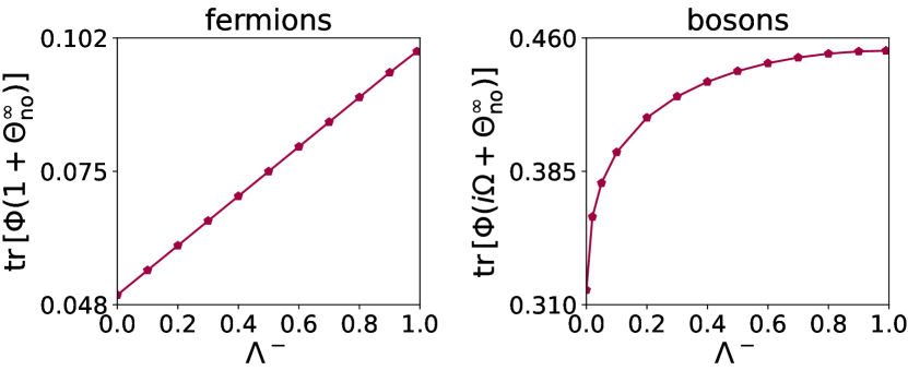
Again, the evolution of the no-jump probability Pno(t)subscript𝑃no𝑡P_{\rm no}(t) is given by Eq. (II.19), where β(t)𝛽𝑡\beta(t) is specified by Eq. (V.19) choosing the - sign. In Appendix D, we show that β(t)𝛽𝑡\beta(t) can also be rewritten in the compact form

β(t)=tr[𝚽(𝟙+𝚯no(t))].𝛽𝑡trace𝚽1subscript𝚯no𝑡\beta(t)=\tr[\bm{\Phi}(\mathds{1}+\bm{\Theta}_{\rm no}(t))\Big{]}. (VII.31)

In the long-time limit,

Pno(t)exp(tr[𝚽(𝟙+𝚯no)]t),t,formulae-sequencesimilar-tosubscript𝑃no𝑡trace𝚽1superscriptsubscript𝚯no𝑡similar-to𝑡P_{\rm no}(t)\sim\exp\left(-\tr\left[\bm{\Phi}(\mathds{1}+\bm{\Theta}_{\rm no}^{\infty})\right]t\right),\qquad t\sim\infty, (VII.32)

where 𝚯nosuperscriptsubscript𝚯no\bm{\Theta}_{\rm no}^{\infty} is the stationary solution of the Riccati equation (VII.2).

VIII No-jump dynamics with pairing terms - bosonic chains

In this section, we focus on the conditional no-jump dynamics of non-interacting bosons with particle non-conserving Hamiltonian operators, in analogy with Sec. VII.

Assuming the 𝒄𝒄\bm{c}’s to be bosonic operators (IV.2), we define the 2L2𝐿2L quadratures,

xn=cn+cn,pn=i(cncn).n=1,,L{x}_{n}={c}_{n}^{\dagger}+c_{n},\qquad{p}_{n}=i({c}_{n}^{\dagger}-{c}_{n}).\qquad n=1,\ldots,L (VIII.1)

which are Hermitian (xk=xksubscript𝑥𝑘superscriptsubscript𝑥𝑘x_{k}=x_{k}^{\dagger}, pk=pksubscript𝑝𝑘superscriptsubscript𝑝𝑘p_{k}=p_{k}^{\dagger}) and satisfy the algebra

[xk,p]=2iδk,[xk,x]=0,[pk,p]=0.formulae-sequencecommutatorsubscript𝑥𝑘subscript𝑝2𝑖subscript𝛿𝑘formulae-sequencecommutatorsubscript𝑥𝑘subscript𝑥0commutatorsubscript𝑝𝑘subscript𝑝0\commutator{x_{k}}{p_{\ell}}=2i\delta_{k\ell},\qquad\commutator{x_{k}}{x_{\ell}}=0,\qquad\commutator{p_{k}}{p_{\ell}}=0. (VIII.2)

Below, we work with the vector 𝑹=(x1,,xL,p1,,pL)superscript𝑹subscript𝑥1subscript𝑥𝐿subscript𝑝1subscript𝑝𝐿{\bm{R}}^{\dagger}=(x_{1},\ldots,x_{L},p_{1},\ldots,p_{L}), which then satisfies

[Ri,Rj]=2iΩij,commutatorsubscript𝑅𝑖subscript𝑅𝑗2𝑖subscriptΩ𝑖𝑗\commutator{R_{i}}{R_{j}}=2i\Omega_{ij}, (VIII.3)

where 𝛀𝛀\bm{\Omega} is the symplectic form

𝛀=(iσy)𝟙L=(0𝟙L𝟙L0),𝛀tensor-product𝑖subscript𝜎𝑦subscript1𝐿matrix0missing-subexpressionsubscript1𝐿missing-subexpressionsubscript1𝐿missing-subexpression0\bm{\Omega}=(i\sigma_{y})\otimes\mathds{1}_{L}=\begin{pmatrix}\mbox{\Large 0}&\vline&\mathds{1}_{L}\\ \hline\cr-\mathds{1}_{L}&\vline&\mbox{\Large 0}\end{pmatrix}, (VIII.4)

𝟙Lsubscript1𝐿\mathds{1}_{L} is the L×L𝐿𝐿L\times L identity matrix and (i𝛀)2=𝟙superscript𝑖𝛀21(i\bm{\Omega})^{2}=\mathds{1}. The most general quadratic Hamiltonian is

H=14𝑹𝓣𝑹,𝐻14superscript𝑹𝓣𝑹H=\frac{1}{4}{\bm{R}}^{\dagger}\cdot\bm{\mathcal{T}}\cdot{\bm{R}}, (VIII.5)

where 𝓣𝓣\bm{\mathcal{T}} is a 2L×2L2𝐿2𝐿2L\times 2L Hermitian matrix. In Appendix E we show that, without loss of generality, we can assume 𝓣𝓣\bm{\mathcal{T}} to be symmetric. Similarly to Appendix C, we can prove that the dissipator (IV.3) may be put in the form

𝒟(ρ)=i,j=12LΥij[RiρRj12{RjRi,ρ}].𝒟𝜌superscriptsubscript𝑖𝑗12𝐿subscriptΥ𝑖𝑗delimited-[]subscript𝑅𝑖𝜌subscript𝑅𝑗12subscript𝑅𝑗subscript𝑅𝑖𝜌\mathcal{D}(\rho)=\sum\limits_{i,j=1}^{2L}\Upsilon_{ij}\Big{[}R_{i}\rho R_{j}-\frac{1}{2}\{R_{j}R_{i},\rho\}\Big{]}. (VIII.6)

The same holds for the partial monitoring dynamics (IV.3),

0(ρ)=i[H,ρ]+i,j=12L[[𝚼𝚽]ijRiρRj(𝚼)ij2{RjRi,ρ}],subscript0𝜌𝑖𝐻𝜌superscriptsubscript𝑖𝑗12𝐿delimited-[]subscriptdelimited-[]𝚼𝚽𝑖𝑗subscript𝑅𝑖𝜌subscript𝑅𝑗subscript𝚼𝑖𝑗2subscript𝑅𝑗subscript𝑅𝑖𝜌\mathcal{L}_{0}({\rho})=-i[{H},{\rho}]+\sum\limits_{i,j=1}^{2L}\Big{[}[\bm{\Upsilon}-\bm{\Phi}]_{ij}R_{i}\rho R_{j}-\frac{(\bm{\Upsilon})_{ij}}{2}\{R_{j}R_{i},\rho\}\Big{]}, (VIII.7)

where 𝚼𝚼\bm{\Upsilon} and 𝚽𝚽\bm{\Phi} are given by Eqs. (VII.6,VII.8), since these matrices are not sensitive to bosonic or fermionic algebra.

VIII.1 Full monitoring

When all channels are perfectly monitored, 𝚲+=𝚲=𝟙superscript𝚲superscript𝚲1\bm{\Lambda}^{+}=\bm{\Lambda}^{-}=\mathds{1} and 𝚼=𝚽𝚼𝚽\bm{\Upsilon}=\bm{\Phi}. The no-jump Liouvillian reduces to

0(ρ)=i[H,ρ]12i,j=12L(𝚼)ij{RjRi,ρ},subscript0𝜌𝑖𝐻𝜌12superscriptsubscript𝑖𝑗12𝐿subscript𝚼𝑖𝑗subscript𝑅𝑗subscript𝑅𝑖𝜌\mathcal{L}_{0}({\rho})=-i[{H},{\rho}]-\frac{1}{2}\sum\limits_{i,j=1}^{2L}(\bm{\Upsilon})_{ij}\{R_{j}R_{i},\rho\}, (VIII.8)

After some algebra, 0subscript0\mathcal{L}_{0} takes the form (II.6) with effective Hamiltonian

He=𝑹𝓣i(𝚼+𝚼T)4𝑹i4tr(𝜸+𝜸).subscript𝐻𝑒superscript𝑹𝓣𝑖𝚼superscript𝚼T4𝑹𝑖4tracesuperscript𝜸superscript𝜸{H}_{e}={\bm{R}}^{\dagger}\cdot\frac{\bm{\mathcal{T}}-i(\bm{\Upsilon}+\bm{\Upsilon}^{{}^{\text{T}}})}{4}\cdot{\bm{R}}-\frac{i}{4}\tr(\bm{\gamma}^{+}-\bm{\gamma}^{-}). (VIII.9)

VIII.2 Dynamics under partial monitoring

We now derive the conditional dynamics under partial monitoring, following closely the calculations (and the notation) of Sec. VII.2. We assume that the initial state is Gaussian. The unconditional dynamics (II.1) with the quadratures (VIII.1), the Hamiltonian (VIII.5), the dissipator (VIII.6) and the matrix (VII.6) is Gaussian preserving, which means

ρ(t):=et(ρ0)=e14𝑹(i𝛀)𝓜t𝑹Zt,assign𝜌𝑡superscript𝑒𝑡subscript𝜌0superscript𝑒14superscript𝑹𝑖𝛀subscript𝓜𝑡𝑹subscript𝑍𝑡{\rho}(t):=e^{\mathcal{L}t}({\rho}_{0})=\frac{e^{\frac{1}{4}{{\bm{R}}}^{\dagger}\cdot(i\bm{\Omega})\bm{\mathcal{M}}_{t}\cdot{\bm{R}}}}{Z_{t}}, (VIII.10)

where (i𝛀)𝓜t𝑖𝛀subscript𝓜𝑡(i\bm{\Omega})\bm{\mathcal{M}}_{t} is Hermitian and symmetric,

Ztsubscript𝑍𝑡\displaystyle Z_{t} =tr{e14𝑹(i𝛀)𝓜t𝑹}=1det(𝟙e𝓜t),absenttracesuperscript𝑒14superscript𝑹𝑖𝛀subscript𝓜𝑡𝑹11superscript𝑒subscript𝓜𝑡\displaystyle=\tr\{e^{\frac{1}{4}{{\bm{R}}}^{\dagger}\cdot(i\bm{\Omega})\bm{\mathcal{M}}_{t}\cdot{\bm{R}}}\Big{\}}=\frac{1}{\sqrt{\det(\mathds{1}-e^{\bm{\mathcal{M}}_{t}})}}, (VIII.11)
e𝓜tsuperscript𝑒subscript𝓜𝑡\displaystyle e^{\bm{\mathcal{M}}_{t}} =𝚯(i𝛀)𝟙𝚯(i𝛀)+𝟙,absent𝚯𝑖𝛀1𝚯𝑖𝛀1\displaystyle=\frac{\bm{\Theta}(i\bm{\Omega})-\mathds{1}}{\bm{\Theta}(i\bm{\Omega})+\mathds{1}}, (VIII.12)

and

𝚯(t)ij𝚯subscript𝑡𝑖𝑗\displaystyle\bm{\Theta}(t)_{ij} =12tr{{Ri,Rj}ρ(t)}=12{Ri,Rj}(t),absent12tracesubscript𝑅𝑖subscript𝑅𝑗𝜌𝑡12delimited-⟨⟩subscript𝑅𝑖subscript𝑅𝑗𝑡\displaystyle=\frac{1}{2}\tr\{\{R_{i},R_{j}\}\rho(t)\Big{\}}=\frac{1}{2}\langle\{R_{i},R_{j}\}\rangle(t), (VIII.13)

is the correlation matrix. The matrix 𝚯𝚯\bm{\Theta} is Hermitian (𝚯=𝚯superscript𝚯𝚯\bm{\Theta}^{\dagger}=\bm{\Theta}) and symmetric (𝚯T=𝚯superscript𝚯T𝚯\bm{\Theta}^{\text{T}}=\bm{\Theta}) as well. It can be proved that the correlation matrix 𝚯𝚯\bm{\Theta} satisfies the Lyapunov differential equation

d𝚯dt=(𝓦𝚯+𝚯𝓦)+𝓕,𝑑𝚯𝑑𝑡𝓦𝚯𝚯superscript𝓦𝓕\frac{d\bm{\Theta}}{dt}=-\big{(}\bm{\mathcal{W}}\bm{\Theta}+\bm{\Theta}\bm{\mathcal{W}}^{\dagger}\big{)}+\bm{\mathcal{F}}, (VIII.14)

with

𝓦𝓦\displaystyle\bm{\mathcal{W}} =𝛀𝓣(i𝛀)(𝚼𝚼T),absent𝛀𝓣𝑖𝛀𝚼superscript𝚼T\displaystyle=-\bm{\Omega}\bm{\mathcal{T}}-(i\bm{\Omega})(\bm{\Upsilon}-\bm{\Upsilon}^{\text{T}}), (VIII.15)
𝓕𝓕\displaystyle\bm{\mathcal{F}} =2(i𝛀)(𝚼T+𝚼)(i𝛀).absent2𝑖𝛀superscript𝚼T𝚼𝑖𝛀\displaystyle=2(i\bm{\Omega})(\bm{\Upsilon}^{\text{T}}+\bm{\Upsilon})(i\bm{\Omega}). (VIII.16)

In Appendix F, we show that the conditional no-jump dynamics is solved by the Gaussian ansatz

ρ~no(t):=e0t(ρ0)=e14𝑹(i𝛀)𝓜tno𝑹ζt,assignsubscript~𝜌no𝑡superscript𝑒subscript0𝑡subscript𝜌0superscript𝑒14superscript𝑹𝑖𝛀superscriptsubscript𝓜𝑡no𝑹subscript𝜁𝑡{\tilde{\rho}}_{\rm no}(t):=e^{\mathcal{L}_{0}t}({\rho}_{0})=\frac{e^{\frac{1}{4}{{\bm{R}}}^{\dagger}\cdot(i\bm{\Omega})\bm{\mathcal{M}}_{t}^{\rm no}\cdot{\bm{R}}}}{\zeta_{t}}, (VIII.17)

for some matrix 𝓜tnosuperscriptsubscript𝓜𝑡no\bm{\mathcal{M}}_{t}^{\rm no} and some c𝑐c-number ζtsubscript𝜁𝑡\zeta_{t}, which must satisfy specific differential equations, to be determined. Again, the properly normalized state is

ρno(t)subscript𝜌no𝑡\displaystyle{\rho}_{\rm no}(t) :=ρ~no(t)Pno(t)=e14𝑹(i𝛀)𝓜tno𝑹Ztno,assignabsentsubscript~𝜌no𝑡subscript𝑃no𝑡superscript𝑒14superscript𝑹𝑖𝛀superscriptsubscript𝓜𝑡no𝑹superscriptsubscript𝑍𝑡no\displaystyle:=\frac{{\tilde{\rho}}_{\rm no}(t)}{P_{\rm no}(t)}=\frac{e^{\frac{1}{4}{{\bm{R}}}^{\dagger}\cdot(i\bm{\Omega})\bm{\mathcal{M}}_{t}^{\rm no}\cdot{\bm{R}}}}{Z_{t}^{\rm no}}, (VIII.18)
Ztnosuperscriptsubscript𝑍𝑡no\displaystyle Z_{t}^{\rm no} =tr(e14𝑹(i𝛀)𝓜tno𝑹)=1det(𝟙e𝓜tno).absenttracesuperscript𝑒14superscript𝑹𝑖𝛀superscriptsubscript𝓜𝑡no𝑹11superscript𝑒subscriptsuperscript𝓜no𝑡\displaystyle=\tr(e^{\frac{1}{4}{{\bm{R}}}^{\dagger}\cdot(i\bm{\Omega})\bm{\mathcal{M}}_{t}^{\rm no}\cdot{\bm{R}}})=\frac{1}{\sqrt{\det(\mathds{1}-e^{\bm{\mathcal{M}}^{\rm no}_{t}})}}. (VIII.19)

The correlation matrix

𝚯no(t)ij=[coth(𝓜tno/2)(i𝛀)]ij=12{Ri,Rj}no(t),subscript𝚯nosubscript𝑡𝑖𝑗subscriptdelimited-[]hyperbolic-cotangentsuperscriptsubscript𝓜𝑡no2𝑖𝛀𝑖𝑗12subscriptdelimited-⟨⟩subscript𝑅𝑖subscript𝑅𝑗no𝑡\bm{\Theta}_{\rm no}(t)_{ij}=-[\coth(\bm{\mathcal{M}}_{t}^{\rm no}/2)\,(i\bm{\Omega})]_{ij}=\frac{1}{2}\langle\{R_{i},R_{j}\}\rangle_{\rm no}(t), (VIII.20)

fully characterizes the normalized state ρno(t)subscript𝜌no𝑡{\rho}_{\rm no}(t). The matrix 𝚯nosubscript𝚯no\bm{\Theta}_{\rm no} can also be put in the same block form (VII.22) with

𝚯1,nosubscript𝚯1no\displaystyle\bm{\Theta}_{1,\rm no} =𝑪noT+𝑪no+𝑺no+𝑺no+𝟙,absentsuperscriptsubscript𝑪noTsubscript𝑪nosubscript𝑺nosuperscriptsubscript𝑺no1\displaystyle=\bm{C}_{\rm no}^{\text{T}}+\bm{C}_{\rm no}+\bm{S}_{\rm no}+\bm{S}_{\rm no}^{\dagger}+\mathds{1}, (VIII.21)
𝚯2,nosubscript𝚯2no\displaystyle\bm{\Theta}_{2,\rm no} =𝑪noT𝑪no𝑺no+𝑺no,absentsuperscriptsubscript𝑪noTsubscript𝑪nosubscript𝑺nosuperscriptsubscript𝑺no\displaystyle=\bm{C}_{\rm no}^{\text{T}}-\bm{C}_{\rm no}-\bm{S}_{\rm no}+\bm{S}_{\rm no}^{\dagger}, (VIII.22)
𝚯3,nosubscript𝚯3no\displaystyle\bm{\Theta}_{3,\rm no} =𝑪noT+𝑪no𝑺no𝑺no+𝟙,absentsuperscriptsubscript𝑪noTsubscript𝑪nosubscript𝑺nosuperscriptsubscript𝑺no1\displaystyle=\bm{C}_{\rm no}^{\text{T}}+\bm{C}_{\rm no}-\bm{S}_{\rm no}-\bm{S}_{\rm no}^{\dagger}+\mathds{1}, (VIII.23)

where

𝑪no(t)ijsubscript𝑪nosubscript𝑡𝑖𝑗\displaystyle\bm{C}_{\rm no}(t)_{ij} =tr{cjciρno(t)}=cjcino(t),absenttracesuperscriptsubscript𝑐𝑗subscript𝑐𝑖subscript𝜌no𝑡subscriptdelimited-⟨⟩superscriptsubscript𝑐𝑗subscript𝑐𝑖no𝑡\displaystyle=\tr\{{c}_{j}^{\dagger}{c}_{i}\leavevmode\nobreak\ {\rho}_{\rm no}(t)\Big{\}}=\langle c_{j}^{\dagger}{c}_{i}\rangle_{{\rm no}}(t), (VIII.24)
𝑺no(t)ijsubscript𝑺nosubscript𝑡𝑖𝑗\displaystyle\bm{S}_{\rm no}(t)_{ij} =tr{cjciρno(t)}=cjcino(t),absenttracesuperscriptsubscript𝑐𝑗superscriptsubscript𝑐𝑖subscript𝜌no𝑡subscriptdelimited-⟨⟩superscriptsubscript𝑐𝑗superscriptsubscript𝑐𝑖no𝑡\displaystyle=\tr\{{c}_{j}^{\dagger}{c}_{i}^{\dagger}\leavevmode\nobreak\ {\rho}_{\rm no}(t)\Big{\}}=\langle c_{j}^{\dagger}{c}_{i}^{\dagger}\rangle_{{\rm no}}(t), (VIII.25)

are L×L𝐿𝐿L\times L matrices. Due to the bosonic commutation rules (IV.2), 𝑪no=𝑪nosubscript𝑪nosuperscriptsubscript𝑪no\bm{C}_{\rm no}=\bm{C}_{\rm no}^{\dagger} and 𝑺no=𝑺noTsubscript𝑺nosuperscriptsubscript𝑺noT\bm{S}_{\rm no}=\bm{S}_{\rm no}^{\text{T}}. As sanity check, we see that 𝚯no=𝚯nosubscript𝚯nosuperscriptsubscript𝚯no\bm{\Theta}_{\rm no}=\bm{\Theta}_{\rm no}^{\dagger} and 𝚯no=𝚯noTsubscript𝚯nosuperscriptsubscript𝚯noT\bm{\Theta}_{\rm no}=\bm{\Theta}_{\rm no}^{\text{T}}.

In Appendix F, we provide two independent differential equations for ζtsubscript𝜁𝑡\zeta_{t} and the conditional covariance matrix 𝚯no(t)subscript𝚯no𝑡\bm{\Theta}_{\rm no}(t),

d𝚯nodt=𝑑subscript𝚯no𝑑𝑡absent\displaystyle\frac{d\bm{\Theta}_{\rm no}}{dt}= (𝓦𝚯no+𝚯no𝓦)+𝓕𝓦subscript𝚯nosubscript𝚯nosuperscript𝓦𝓕\displaystyle-\big{(}\bm{\mathcal{W}}\bm{\Theta}_{\rm no}+\bm{\Theta}_{\rm no}\bm{\mathcal{W}}^{\dagger}\big{)}+\bm{\mathcal{F}}
(i𝛀𝚯no)𝚽T(i𝛀𝚯no)𝑖𝛀subscript𝚯nosuperscript𝚽T𝑖𝛀subscript𝚯no\displaystyle-(i\bm{\Omega}-\bm{\Theta}_{\rm no})\,\bm{\Phi}^{\text{T}}\,(i\bm{\Omega}-\bm{\Theta}_{\rm no})
(i𝛀+𝚯no)𝚽(i𝛀+𝚯no),𝑖𝛀subscript𝚯no𝚽𝑖𝛀subscript𝚯no\displaystyle-(i\bm{\Omega}+\bm{\Theta}_{\rm no})\,\bm{\Phi}\,(i\bm{\Omega}+\bm{\Theta}_{\rm no}), (VIII.26)
ddtln(ζ)t=𝑑𝑑𝑡subscript𝜁𝑡absent\displaystyle\frac{d}{dt}\ln{\zeta}_{t}= tr(𝚼(i𝛀)+[𝚼𝚽]𝚯no(i𝛀)+𝟙𝚯no(i𝛀)𝟙(i𝛀)missing),trace𝚼𝑖𝛀delimited-[]𝚼𝚽subscript𝚯no𝑖𝛀1subscript𝚯no𝑖𝛀1𝑖𝛀missing\displaystyle\tr\bigg(\bm{\Upsilon}(i\bm{\Omega})+[\bm{\Upsilon}-\bm{\Phi}]\frac{\bm{\Theta}_{\rm no}(i\bm{\Omega})+\mathds{1}}{\bm{\Theta}_{\rm no}(i\bm{\Omega})-\mathds{1}}(i\bm{\Omega})\bigg{missing}), (VIII.27)

where 𝓦𝓦\bm{\mathcal{W}} and 𝓕𝓕\bm{\mathcal{F}} are the matrices into Eqs. (VIII.15,VIII.16), while 𝚼𝚼\bm{\Upsilon} and 𝚽𝚽\bm{\Phi} are specified by Eqs. (VII.6,VII.8). Eq. (VIII.2) is again a Riccati-type equation and represents another important result of this work. Eq. (VIII.2) generalizes Eq. (V.2) for bosonic chains with particle non-conserving Hamiltonians. If there is no monitoring, 𝚲+=𝚲=0superscript𝚲superscript𝚲0\bm{\Lambda}^{+}=\bm{\Lambda}^{-}=0, 𝚯no=𝚯subscript𝚯no𝚯\bm{\Theta}_{\rm no}=\bm{\Theta} and we recover the Lyapunov equation (VIII.14) for the unconditional dynamics.
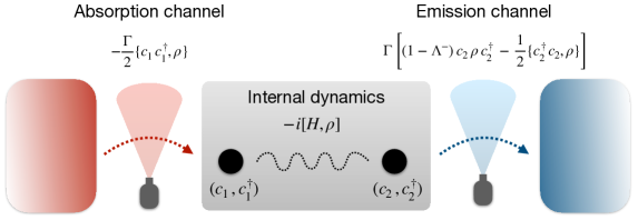
Refer to caption
Figure 8: Sketch of the 2-body problem: we study the no-jump dynamics (IX.1) for a boundary driven system, which undergoes a non-ideal measurement process on the emission channel, with monitoring efficiency ΛsuperscriptΛ\Lambda^{-}. The internal dynamics is generated by the Hamiltonian H𝐻H, which takes the form (IX.2) for fermions and the form (IX.3) for bosons.

When 𝚲+=𝚲=𝟙superscript𝚲superscript𝚲1\bm{\Lambda}^{+}=\bm{\Lambda}^{-}=\mathds{1}, Eq. (VIII.2) can also be written more compactly as

d𝚯nodt=𝚯no𝓣𝛀(𝓣𝛀)T𝚯no+12𝓕12𝚯no(i𝛀)𝓕(i𝛀)𝚯no.𝑑subscript𝚯no𝑑𝑡subscript𝚯no𝓣𝛀superscript𝓣𝛀Tsubscript𝚯no12𝓕12subscript𝚯no𝑖𝛀𝓕𝑖𝛀subscript𝚯no\frac{d\bm{\Theta}_{\rm no}}{dt}=-\bm{\Theta}_{\rm no}\bm{\mathcal{T}}\bm{\Omega}-(\bm{\mathcal{T}}\bm{\Omega})^{\text{T}}\bm{\Theta}_{\rm no}+\frac{1}{2}\bm{\mathcal{F}}-\frac{1}{2}\bm{\Theta}_{\rm no}(i\bm{\Omega})\bm{\mathcal{F}}(i\bm{\Omega})\bm{\Theta}_{\rm no}. (VIII.28)

The evolution of the no-jump probability Pno(t)subscript𝑃no𝑡P_{\rm no}(t) is given by Eq. (II.19), where β(t)𝛽𝑡\beta(t) is specified by Eq. (V.19) choosing the ++ sign. In Appendix F, we show that β(t)𝛽𝑡\beta(t) can also be rewritten in the compact form

β(t)=tr[𝚽(i𝛀+𝚯no(t))].𝛽𝑡trace𝚽𝑖𝛀subscript𝚯no𝑡\beta(t)=\tr[\bm{\Phi}(i\bm{\Omega}+\bm{\Theta}_{\rm no}(t))\Big{]}. (VIII.29)

In the long-time limit,

Pno(t)exp(tr[𝚽(i𝛀+𝚯no)]t),t,formulae-sequencesimilar-tosubscript𝑃no𝑡trace𝚽𝑖𝛀superscriptsubscript𝚯no𝑡similar-to𝑡P_{\rm no}(t)\sim\exp\left(-\tr\left[\bm{\Phi}(i\bm{\Omega}+\bm{\Theta}_{\rm no}^{\infty})\right]t\right),\qquad t\sim\infty, (VIII.30)

where 𝚯nosuperscriptsubscript𝚯no\bm{\Theta}_{\rm no}^{\infty} is the stationary solution of the Riccati equation (VIII.2).

Sec. VIII concludes the study of the conditional no-jump dynamics of non-interacting quantum chains. In the next section, we shall consider a specific setting where we all the analytical results provided in this work can be successfully applied.

IX Example: boundary driven system

As an application of the no-jump dynamics with pairing terms (see Sec. VII and Sec. VIII), we study a simple boundary driven system of bosons (B) and fermions (F). More specifically, we couple a 2-site system to two reservoirs, with an absorption channel on site 111 and an emission channel on site 222. We assume jump rates Γ1+=Γ2=ΓsubscriptsuperscriptΓ1subscriptsuperscriptΓ2Γ\Gamma^{+}_{1}=\Gamma^{-}_{2}=\Gamma and two local detectors for the particle exchange. In particular, we assume the detector on the hot bath to work with perfect efficiency Λ+=1superscriptΛ1\Lambda^{+}=1 and the other one on the cold reservoir with efficiency Λ(0,1)superscriptΛ01\Lambda^{-}\in(0,1). The goal is to study the no-jump dynamics generated by the dynamical map

0(ρ)=i[H,ρ]Γ2{c1c1,ρ}+Γ[(1Λ)c2ρc212{c2c2,ρ}],subscript0𝜌𝑖𝐻𝜌Γ2subscript𝑐1superscriptsubscript𝑐1𝜌Γdelimited-[]1superscriptΛsubscript𝑐2𝜌superscriptsubscript𝑐212superscriptsubscript𝑐2subscript𝑐2𝜌\mathcal{L}_{0}({\rho})=-i[{H},{\rho}]-\frac{\Gamma}{2}\{c_{1}c_{1}^{\dagger},\rho\}+\Gamma\left[(1-\Lambda^{-})\,c_{2}\rho c_{2}^{\dagger}-\frac{1}{2}\{c_{2}^{\dagger}c_{2},\rho\}\right], (IX.1)

where H𝐻H is the prototypical Hamiltonian

H=𝐻absent\displaystyle H= c1c2+c2c1+g(c1c2c1c2),(F)superscriptsubscript𝑐1subscript𝑐2superscriptsubscript𝑐2subscript𝑐1𝑔subscript𝑐1subscript𝑐2superscriptsubscript𝑐1superscriptsubscript𝑐2(F)\displaystyle\,c_{1}^{\dagger}c_{2}+c_{2}^{\dagger}c_{1}+g(c_{1}c_{2}-c_{1}^{\dagger}c_{2}^{\dagger}),\hskip 36.98866pt\text{(F)} (IX.2)
H=𝐻absent\displaystyle H= c1c2+c2c1+g(c1c2+c1c2),(B)superscriptsubscript𝑐1subscript𝑐2superscriptsubscript𝑐2subscript𝑐1𝑔subscript𝑐1subscript𝑐2superscriptsubscript𝑐1superscriptsubscript𝑐2(B)\displaystyle\,c_{1}^{\dagger}c_{2}+c_{2}^{\dagger}c_{1}+g(c_{1}c_{2}+c_{1}^{\dagger}c_{2}^{\dagger}),\hskip 36.98866pt\text{(B)} (IX.3)

and g𝑔g is the amplitude of the pairing terms. The full experimental setup is schematically represented in Fig. 8. As usual, we aim to compute the no-jump probability

Pno(t)={exp(0t𝑑str[𝚽(𝟙+𝚯no(s))]),(F)exp(0t𝑑str[𝚽(i𝛀+𝚯no(s))]),(B)subscript𝑃no𝑡casessuperscriptsubscript0𝑡differential-d𝑠trace𝚽1subscript𝚯no𝑠(F)otherwiseotherwiseotherwisesuperscriptsubscript0𝑡differential-d𝑠trace𝚽𝑖𝛀subscript𝚯no𝑠(B)otherwiseP_{\rm no}(t)=\begin{cases}\exp\left(-\int_{0}^{t}ds\,\tr[\bm{\Phi}\bigg{(}\mathds{1}+\bm{\Theta}_{\rm no}(s)\bigg{)}\,\bigg{]}\,\right),\hskip 42.67912pt\text{(F)}\\ \\ \exp\left(-\int_{0}^{t}ds\,\tr[\bm{\Phi}\bigg{(}i\bm{\Omega}+\bm{\Theta}_{\rm no}(s)\bigg{)}\,\bigg{]}\,\right),\hskip 36.98866pt\text{(B)}\end{cases} (IX.4)

and the WTDs

W(2,)(t)subscript𝑊2𝑡\displaystyle W_{(2,-)}(t) =ΓΛPno(t)c2c2no(t)absentΓsuperscriptΛsubscript𝑃no𝑡subscriptdelimited-⟨⟩superscriptsubscript𝑐2subscript𝑐2no𝑡\displaystyle=\Gamma\Lambda^{-}P_{\rm no}(t)\,\langle c_{2}^{\dagger}c_{2}\rangle_{\rm no}(t)
=ΓΛPno(t)×{12(1+i𝚯no(t)24),(F)14(𝚯no(t)22+𝚯no(t)442),(B)absentΓsuperscriptΛsubscript𝑃no𝑡cases121𝑖subscript𝚯nosubscript𝑡24(F)otherwiseotherwiseotherwise14subscript𝚯nosubscript𝑡22subscript𝚯nosubscript𝑡442(B)otherwise\displaystyle=\Gamma\Lambda^{-}P_{\rm no}(t)\times\begin{cases}\,\frac{1}{2}\left(1+i\bm{\Theta}_{\rm no}(t)_{24}\right),\hskip 51.21504pt\text{(F)}\\ \\ \,\frac{1}{4}\left(\bm{\Theta}_{\rm no}(t)_{22}+\bm{\Theta}_{\rm no}(t)_{44}-2\right),\hskip 9.95863pt\text{(B)}\end{cases} (IX.5)
W(1,+)(t)subscript𝑊1𝑡\displaystyle W_{(1,+)}(t) =ΓPno(t)c1c1no(t)absentΓsubscript𝑃no𝑡subscriptdelimited-⟨⟩subscript𝑐1superscriptsubscript𝑐1no𝑡\displaystyle=\Gamma P_{\rm no}(t)\,\langle c_{1}c_{1}^{\dagger}\rangle_{\rm no}(t)
=ΓPno(t)×{12(1i𝚯no(t)13),(F)14(𝚯no(t)11+𝚯no(t)33+2),(B)absentΓsubscript𝑃no𝑡cases121𝑖subscript𝚯nosubscript𝑡13(F)otherwiseotherwiseotherwise14subscript𝚯nosubscript𝑡11subscript𝚯nosubscript𝑡332(B)otherwise\displaystyle=\Gamma P_{\rm no}(t)\times\begin{cases}\,\frac{1}{2}\left(1-i\bm{\Theta}_{\rm no}(t)_{13}\right),\hskip 51.21504pt\text{(F)}\\ \\ \,\frac{1}{4}\left(\bm{\Theta}_{\rm no}(t)_{11}+\bm{\Theta}_{\rm no}(t)_{33}+2\right),\hskip 9.95863pt\text{(B)}\end{cases} (IX.6)

which are formulated in terms of the 4×4444\times 4 correlation matrix 𝚯𝚯\bm{\Theta}, whose definition and dynamics are given by Eqs. (VII.21,VII.2) for fermions and Eqs. (VIII.20,VIII.2) for bosons. We remember that Pno(t)subscript𝑃no𝑡P_{\rm no}(t) is the probability of not detecting any jump in [0,t]0𝑡[0,t], while W(2,)(t)subscript𝑊2𝑡W_{(2,-)}(t) and W(1,+)(t)subscript𝑊1𝑡W_{(1,+)}(t) are the probability distributions to observe the first jump in the channel (2,)2(2,-) and (1,+)1(1,+), respectively. Due to the normalization condition, the WTDs satisfy

0𝑑t(W(1,+)(t)+W(2,)(t))=1.superscriptsubscript0differential-d𝑡subscript𝑊1𝑡subscript𝑊2𝑡1\int_{0}^{\infty}dt\,\left(W_{(1,+)}(t)+W_{(2,-)}(t)\right)=1. (IX.7)

We assume the system is initially prepared in the vacuum state |00ket00\ket{00}, that is a Gaussian state and hence we can apply the theoretical results of Sec. VII and Sec. VIII.
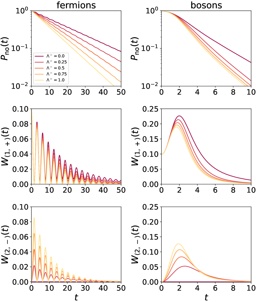
Refer to caption
Figure 9: Conditional dynamics (IX.1) for a quantum chain of non-interacting particles (fermionic and bosonic case), Γ=0.1Γ0.1\Gamma=0.1, g=1𝑔1g=1 and monitoring efficiency Λ={0,0.25,0.5,0.75,1}superscriptΛ00.250.50.751\Lambda^{-}=\{0,0.25,0.5,0.75,1\}. The no-jump probability and the WTDs always show an exponential decay.
Refer to caption
Figure 10: We show the coefficient governing the exponential decay of the no-jump probability (IX.4) and the WTDs (IX,IX), as a function of the monitoring efficiency ΛsuperscriptΛ\Lambda^{-} (bosonic and fermionic case).

In Fig. 9, we show the no-jump probability (IX.4) and the WTDs (IX,IX) for Γ=0.1Γ0.1\Gamma=0.1, g=1𝑔1g=1 and different values of the monitoring efficiency ΛsuperscriptΛ\Lambda^{-}. The two columns refer to the fermionic and bosonic dynamics, respectively. The no-jump probability is a decreasing function of ΛsuperscriptΛ\Lambda^{-}; the higher the monitoring efficiency, more likely particle loss events are detected. If the bosonic WTDs show a fast decay, revealing that the system quickly reaches a stationary regime where the pair creation-annihilation processes are balanced by the non-detected emissions, the fermionic WTDs exhibit a damped oscillatory behaviour with the same periodicity of the local occupation, with maxima and minima reflecting the back and forth motion of the particle along the system. The exponential decay of Pno(t)subscript𝑃no𝑡P_{\rm no}(t), as well as the decay of W(1,+)(t)subscript𝑊1𝑡W_{(1,+)}(t) and W(2,)(t)subscript𝑊2𝑡W_{(2,-)}(t), may be extrapolated from the stationary state, characterized by 𝚯nosuperscriptsubscript𝚯no\bm{\Theta}_{\rm no}^{\infty}, which always exists except for the fermionic case under perfect monitoring (Λ=1superscriptΛ1\Lambda^{-}=1). In addition, for the sake of completeness, Fig. 10 shows tr[𝚽(𝟙+𝚯no)]trace𝚽1superscriptsubscript𝚯no\tr[\bm{\Phi}\big{(}\mathds{1}+\bm{\Theta}_{\rm no}^{\infty}\big{)}\,\big{]} and tr[𝚽(i𝛀+𝚯no)]trace𝚽𝑖𝛀superscriptsubscript𝚯no\tr[\bm{\Phi}\big{(}i\bm{\Omega}+\bm{\Theta}_{\rm no}^{\infty}\big{)}\,\big{]} as a function of the parameter ΛsuperscriptΛ\Lambda^{-}, which are the coefficients governing the exponential decay of the fermionic and bosonic no-jump probabilities; since the results in Fig. 10 are the numerical solutions of highly nonlinear equations, the functions tr[𝚽(𝟙+𝚯no)]trace𝚽1superscriptsubscript𝚯no\tr[\bm{\Phi}\big{(}\mathds{1}+\bm{\Theta}_{\rm no}^{\infty}\big{)}\,\big{]} and tr[𝚽(i𝛀+𝚯no)]trace𝚽𝑖𝛀superscriptsubscript𝚯no\tr[\bm{\Phi}\big{(}i\bm{\Omega}+\bm{\Theta}_{\rm no}^{\infty}\big{)}\,\big{]} are difficult to handle. However, Fig. 10 apparently shows a linear growth for tr[𝚽(𝟙+𝚯no)]trace𝚽1superscriptsubscript𝚯no\tr[\bm{\Phi}\big{(}\mathds{1}+\bm{\Theta}_{\rm no}^{\infty}\big{)}\,\big{]} as a function of ΛsuperscriptΛ\Lambda^{-}. In any case, the decay coefficient is increasing with ΛsuperscriptΛ\Lambda^{-}, as we expect if approaching the ideal monitoring regime.

X Discussion and conclusion

This work aims to be a complete guide to the conditional no-jump dynamics of free particles, providing analytical results for the no-jump probability and the WTDs.

After presenting generic results, we computed the no-jump dynamics of single qubits, either incoherently or coherently driven, whose time evolution turns to be very involved.

As a main result, we successfully generalized the findings into Ref. landi2021waiting, deriving analytical results for the conditional no-jump dynamics of non-interacting chains under inhomogeneous one-body gain-loss processes. We also studied both bosonic and fermionic chains with particle non-conserving Hamiltonian operators. The hypothesis of Gaussianity is crucial to solve the no-jump dynamics, which turns to be governed by a Riccati-type differential equation for the correlation matrix. The solution of the Riccati equation gives access to the no-jump probability and the WTDs. As an example, we studied a tight-binding model with specific gain-loss profiles and finally we moved to boundary driven systems with pairing terms in the Hamiltonian operator. Generalizing the findings into Ref. landi2021waiting to non-interacting bosons also paves the way to quantum optics, with applications in optomechanical systems aspelmeyer2014cavity; bowen2015quantum.

Acknowledgments

The authors acknowledge the financial support the French ANR funding UNIOPEN (Grant No. ANR-22-CE30-0004-01). M.C. thanks the LUE for funding a travel grant (Aide à la mobilité internationale DrEAM).

Appendix A. No-jump dynamics without pairing terms: explicit solution

In this section, we assume the system is prepared in a Gaussian state and we solve the no-jump dynamics generated by (IV.3). To compute dρ~no/dt𝑑subscript~𝜌no𝑑𝑡d{\tilde{\rho}}_{\rm no}/dt we make use of the BCH formula

deK(t)dt={dKdt+12![K,dKdt]+13![K,[K,dKdt]]+}eK,𝑑superscript𝑒𝐾𝑡𝑑𝑡𝑑𝐾𝑑𝑡12𝐾𝑑𝐾𝑑𝑡13𝐾𝐾𝑑𝐾𝑑𝑡superscript𝑒𝐾\frac{de^{K(t)}}{dt}=\left\{\frac{dK}{dt}+\frac{1}{2!}\left[K,\frac{dK}{dt}\right]+\frac{1}{3!}\left[K,\left[K,\frac{dK}{dt}\right]\right]+\ldots\right\}e^{K}, (A.1)

for any Hilbert operator K𝐾K. Combining the BCH formula, the Gaussian ansatz (V.11) and the result

[𝒄𝑿𝒄,𝒄𝒀𝒄]=𝒄[𝑿,𝒀]𝒄.superscript𝒄𝑿𝒄superscript𝒄𝒀𝒄superscript𝒄𝑿𝒀𝒄[{{\bm{c}}}^{\dagger}\cdot\bm{X}\cdot{\bm{c}},\leavevmode\nobreak\ {{\bm{c}}}^{\dagger}\cdot\bm{Y}\cdot{\bm{c}}]={{\bm{c}}}^{\dagger}\cdot[\bm{X},\bm{Y}]\cdot{\bm{c}}. (A.2)

we get

ddte𝒄𝑴tno𝒄=𝒄(de𝑴tnodte𝑴tno)𝒄e𝒄𝑴tno𝒄.𝑑𝑑𝑡superscript𝑒superscript𝒄superscriptsubscript𝑴𝑡no𝒄superscript𝒄𝑑superscript𝑒subscriptsuperscript𝑴no𝑡𝑑𝑡superscript𝑒subscriptsuperscript𝑴no𝑡𝒄superscript𝑒superscript𝒄superscriptsubscript𝑴𝑡no𝒄\frac{d}{dt}e^{-{\bm{c}}^{\dagger}\cdot{\bm{M}}_{t}^{\rm no}\cdot\bm{c}}={{\bm{c}}}^{\dagger}\cdot\left(\frac{de^{-\bm{M}^{\rm no}_{t}}}{dt}e^{\bm{M}^{\rm no}_{t}}\right){\bm{c}}\leavevmode\nobreak\ e^{-{\bm{c}}^{\dagger}\cdot{\bm{M}}_{t}^{\rm no}\cdot\bm{c}}. (A.3)

Hence

dρ~nodt=[𝒄(de𝑴tnodte𝑴tno)𝒄ddtln(ζ)t]ρ~no.𝑑subscript~𝜌no𝑑𝑡delimited-[]superscript𝒄𝑑superscript𝑒subscriptsuperscript𝑴no𝑡𝑑𝑡superscript𝑒subscriptsuperscript𝑴no𝑡𝒄𝑑𝑑𝑡subscript𝜁𝑡subscript~𝜌no\frac{d{\tilde{\rho}}_{\rm no}}{dt}=\left[{\bm{c}}^{\dagger}\cdot\left(\frac{de^{-\bm{M}^{\rm no}_{t}}}{dt}e^{\bm{M}^{\rm no}_{t}}\right){\bm{c}}-\frac{d}{dt}\ln{\zeta}_{t}\right]{\tilde{\rho}}_{\rm no}. (A.4)

Next, we compute 0(ρ~no)subscript0subscript~𝜌no\mathcal{L}_{0}({\tilde{\rho}}_{\rm no}). We use the BCH formulas

e𝒄𝑴tno𝒄𝒄superscript𝑒superscript𝒄superscriptsubscript𝑴𝑡no𝒄𝒄\displaystyle e^{-{\bm{c}}^{\dagger}\cdot{\bm{M}}_{t}^{\rm no}\cdot\bm{c}}{\bm{c}} =(e𝑴tno𝒄)e𝒄𝑴tno𝒄,absentsuperscript𝑒subscriptsuperscript𝑴no𝑡𝒄superscript𝑒superscript𝒄superscriptsubscript𝑴𝑡no𝒄\displaystyle=(e^{\bm{M}^{\rm no}_{t}}{\bm{c}})\leavevmode\nobreak\ e^{-{\bm{c}}^{\dagger}\cdot{\bm{M}}_{t}^{\rm no}\cdot\bm{c}}, (A.5)
e𝒄𝑴tno𝒄𝒄superscript𝑒superscript𝒄superscriptsubscript𝑴𝑡no𝒄superscript𝒄\displaystyle e^{-{\bm{c}}^{\dagger}\cdot{\bm{M}}_{t}^{\rm no}\cdot\bm{c}}{\bm{c}}^{\dagger} =(𝒄e𝑴tno)e𝒄𝑴tno𝒄.absentsuperscript𝒄superscript𝑒subscriptsuperscript𝑴no𝑡superscript𝑒superscript𝒄superscriptsubscript𝑴𝑡no𝒄\displaystyle=({\bm{c}}^{\dagger}e^{-\bm{M}^{\rm no}_{t}})\leavevmode\nobreak\ e^{-{\bm{c}}^{\dagger}\cdot{\bm{M}}_{t}^{\rm no}\cdot\bm{c}}. (A.6)

to push the factors of e𝒄𝑴tno𝒄superscript𝑒superscript𝒄superscriptsubscript𝑴𝑡no𝒄e^{-{\bm{c}}^{\dagger}\cdot{\bm{M}}_{t}^{\rm no}\cdot\bm{c}} to the right. This leads to the following list of factors: {IEEEeqnarray}rCl [H, ~ρ_no] &= c^†⋅( h - e^-M^no_t h e^M^no_t)c   ~ρ_no,
∑_ij [γ^-(1-λ^-)]_ij c_j ~ρ_no c_i^†= ∓c^†⋅(e^-M^no_t γ^-(1-λ^-) )c  ~ρ_no +tr(γ^-(1-λ^-) e^-M^no_tmissing) ~ρ_no,
∑_ij (γ)_ij^- {c_i^†c_j , ~ρ_no} = c^†⋅[ γ^- + e^-M^no_t γ^- e^M^no_t ]c  ~ρ_no,
∑_ij [γ

Conversion to HTML had a Fatal error and exited abruptly. This document may be truncated or damaged.