Abstract
After 25 years of the prediction of the possibility of observations, and despite the many hundred of well studied transiting exoplanet systems, we are still waiting for the announcement of the first confirmed exomoon. Following the “cascade” structure of the Drake-equation, but applied to the existence of an observable exomoon instead the original scope of extraterrestrial intelligence. The scope of this paper is to reveal the structure of the problem, rather than giving a quantitative solution. We identify three important steps that can lead us to the discovery. The steps are the formation, the orbital dynamics and long-term stability, and the observability of a given exomoon in a given system. This way, the question will be closely related to questions of star formation, planet formation, 5 possible pathways of moon formation; long-term dynamics of evolved planet systems involving stellar and planetary rotation and internal structure; and the proper evaluation of the observed data, taken the correlated noise of stellar and instrumental origin and the sampling function also into account. This way, a successful exomoon observation and the interpretations of the expectable further measurements proves to be among the most complex and most interdisciplinary questions in astrophysics.
keywords:
planets and satellites: detection; planets and satellites: formation; techniques: photometric1 \issuenum1 \articlenumber0 \datereceived \daterevised \dateaccepted \datepublished \hreflinkhttps://doi.org/ \TitleThe “Drake equation” of exomoons – a cascade of formation, stability and detection \TitleCitationThe Drake equation of exomoons \AuthorGyula Szabó M. 1,2\orcidA, Jean Schneider 3 \orcidB, Zoltán Dencs1,2,4 and Szilárd Kálmán 2,5,6\orcidD \AuthorNamesGyula Szabó M. \AuthorCitationSzabó, Gy. M. \corresCorrespondence: szgy@gorhard.hu
1 Introduction
We would like to describe briefly the astronomical picture connected with the existence and the detection of an exomoon, which help us in our search for satellites in distant solar systems. The fast progress of exoplanet discoveries (Mayor and Queloz, 1995; Charbonneau et al., 2002; Moutou et al., 2013; Mullally et al., 2015; Ricker et al., 2015; Benz et al., 2021) has inspired a significant interest as to whether these planets can host a detectable moon Sartoretti and Schneider (1999); Szabó et al. (2006); Simon et al. (2007); Kipping (2009). Although no exomoon has been confirmed by date, the foreseeable observation of the exoplanets’ companions will be of high interest because of a few particular reasons:
-
•
They reveal the internal structure of protoplanetary disks during the planet formation and the secondary planetesimal formation scenarios is the protoplanetary disks
- •
- •
- •
The lack of any undoubtedly confirmed exomoon (a moon orbiting an exoplanet, e.g. Sartoretti and Schneider, 1999; Szabó et al., 2006; Simon et al., 2007; Kipping, 2009) to date appears as a confounding conundrum of exoplanet astronomy. The power of space telescopes would enable the detection of smaller bodies than Earth in transits (e.g. Kepler-42 b has a radius of 0.57R⊕, Muirhead et al., 2012), within the size range where moons surely exist – at least in our Solar System. Similarly large moons that seen in our Solar System can be regularly formed in extrasolar systems as well (Malamud et al., 2020), while we do have the appropriate instruments for their detection. The problem of the lacking known exomoons therefore requires a dedicated explanation.
An already propagating naming convention is that if a companion is so large that it is just a few factors smaller than the host planet, they can be named as “binary planets” as well Cabrera and Schneider (2007). There could also be moons orbiting free-floating exoplanets, as suggested by Roccetti et al. (2023); Sajadian and Sangtarash (2023).
In this paper, we review the complex processes that lead to a successful discovery of an exomoon. We interpret this detection as the result of an event cascade where every step must be accomplished successfully. The key steps in this sequence are:
-
1.
Formation of an enough large moon around a planet;
-
2.
Dynamical survival from its formation until our observation;
-
3.
Proper instrument and a verified search strategy that is decisive at the actual system parameters.
All these steps are extended fields to research in their own. However, they are related in a very specific manner, and the discovery of the first exomoon will fully integrate these disciplines. Therefore, it is timely to examine them in respect to their interrelations, and to present the structure of the problem.
In the analysis of this structure, we follow the methodology of describing the event cascade in multiplicative probability terms, just as in the case of the Drake-equation (Drake, 1961). Similarly to the Drake-problem, we do not want to quantitatively estimate the probability of a successful exomoon detection; we rather represent the actors in the problem, with the intention to show how the different steps has to be considered while planning exomoon-discovering strategies.
The paper is organized as follows. Section 2 exposes the cascade equation, and explains its terms and their domains. Section 3 reviews key points of our current understanding of the formation, survival and observation aspects in three subsections, while Section 4 discusses the results in the light of how a habitable moon can be discovered.
2 The cascade equation of the problem
To express our chances for a successful detection of a moon in an exoplanet system we sketch up the following equation:
| (1) |
where expresses the expectation number of our confirmed exomoon observations; is the exoplanets we observed with the appropriate technique (e.g. in transit if considering moon detection in transit light curves). The cascade terms are , which denotes the fraction of moons forming in planet systems in general; , expressing the fraction of moons surviving by the time of our observation; and , which is the probability of an observation of the system with our strategy – likely involving current state-of-the-art equipments.
Equation 1 has a similar structure to the Drake-equation: it builds up an event cascade leading to a successful discovery, consisting of conditional probabilities; and also assumes the independence of the consecutive factors. Another similarity is that the task of Equation 1 is to show the structure of the problem, in an epistemological context, and not the quantitative estimate itself directly. Eq. 1 assumes a reasonable event cascade leading to a moon detection, since the moon has to be formed first, then remain on stable orbit until the observations, and then the observation has to be performed: there is no way to observe a non-existing or an escaped moon. But the factors surely depend on several system parameters and on the search strategy, and hence, the factors are not independent either from each other.
Therefore, the different factors will be functions of various system parameters (parameters of the moon and the planet–star system), and is also a function of the observation strategy (instrument, methods, detection limits, etc.) applied to quest the exomoons in the general case.
Let’s denote the parameters of the star and the planet with , the parameters of the moon with , the parameters of the instrument and searching strategy with . We can now write:
| (2) |
Here the integration goes over a set of relevant system parameters , covering an integration volume of a range . This integral expresses how the three different fields of astrophysics and instrumentation are interrelated to each other. The enclosed integral is the estimator of a expectation number of an observable moon in a given system, and the summation outside the integral sums up for all the known systems. Because the set of known planet–moon systems will always be finite, we can consider the individual systems by each, take the relevant system parameters into account as the conditions within the integral, and then, sum up for all the known planets.
2.1 The parameter domain
In the general case, the parameter space is spanned by many variables, including the stellar mass, age, , metallicity, abundance of refractory elements, stellar rotation rate; the six orbital elements of the planet, the planet’s mass and radius, its tidal constant, its rotation period; which are known parameters (values with priors). The parameters related to the moon are also part of the parameter domain, but these are eventually unknowns, and the integral has to cover them within a wide range. These include six independent orbital elements of the moon, its mass and size. These are 24 independent variables, and the integral will run above at least 8 variables Simon et al. (2010).
For calculations covering a long time-span, e.g. when estimating the number of observable moons within an open cluster where even the exoplanets are not known (although we have priors for their occurrence), the complete 24 dimensional space Simon et al. (2010) has to be taken as parameters of integration in Eq. 2. Here, the orbital elements of the moon and the planet, and the rotation rate of all the three bodies will be a function of time, described by the equations of the general three-body problem involving tidal interactions (e.g. Sasaki et al., 2012)and the equations of Sasaki (REF), and has to be calculated as a solution of a set of differential equations for each simulations. Tidal constants of the star and the planet also evolve in time. In the most general case, we have a parameter set of 24 dimensions, and 14 of these parameters are time-dependent. Running full simulations are therefore almost impossible because of the too many dimensions, and the time dependencies.
The first question is the identification of the relevant subspace of . Also, the relevant volume where the integrand is non-zero can be well constrained: if one of the factors is for a range of parameters, it makes any further considerations irrelevant in that parameter range. A zeroed factor describes moons that cannot form, or/and cannot survive, or/and cannot be observed, and they do not offer any chance for a detection. This criterion filters out most of the known exoplanets for an exomoon discovery, which shows why we have not succeed in a confirmed discovery of an exomoon yet. This is the task of the present contribution.
3 The formation term
There are many formation scenarios known for how the moons can be formed. The suggested moon formation scenarios are very diverse, and most of the multifaceted scenarios entirely depend on the star formation and planet formation processes. The most important unsolved questions, related to the occurrence of observable moons nowadays, is the followings:
-
1.
What is the most effective way of moon formation? What is the maximum number of moons to form and their maximum possible size?
-
2.
What are the best initial conditions that maximize the later survival chance of the moons?
-
3.
What are the stellar and planet properties that are characteristic for an increased exomoon occurrence, especially the presence of large moons?
-
4.
All discussed scenarios have to be compatible to the presence of the moons in the Solar System, without assuming too specific circumstances during their formation (and hence, following the Copernican Principle).
3.1 Regular satellites
Regular moons form around the circumplanetary material before or slightly after the formation of the planet itself. The irregular moons can be formed in several other kind of moon formation scenarios, such as gravitational capture and secondary moon formation in rings. The possible mechanisms are well reviewed by Heller and Barnes (2013) and Heller et al. (2014), who consider the possible formation mechanisms to lead to regular and irregular satellites, and give a review of the potential habitability of these moons. Here we compare the possible scenaios in Table 1.
The formation of regular moons, similarly to the case of the planets, relies on two different scenarios of core accretion and hydrodynamical disk instabilities, or even, the mixture of both. Here, different pathways of formation have been recognized. During the core-accretion, gravitational perturbations between planet embryos imply a series of constructive impacts up to the formation of a fully grown planet. Three different main scenarios have been proposed to describe the details of this process.
3.1.1 Solids-enhanced subnebula model
This model assumes the formation of a subnebula Mosqueira and Estrada (2003); Estrada et al. (2009). This is composed by an optically thick inner region inside the planet’s centrifugal radius (where the specific angular momentum of the collapsing giant planet gaseous envelope achieves centrifugal balance, located at for Jupiter and for Saturn), and the gas-to-dust ratio, around 100/1, is compatible to what is “usually seen” at many places in the Universe. The subnebula appears at the early stages of planet formation. The outer region of the subnebula extends to a fraction of the Roche lobe, usually is assumed. Both regions can form large moons (e.g. Io, Europa and Ganymede is assumed to have formed in the inner region, while Callisto formed in the outer region). The formation is faster in the inner region. The environment is weakly turbulent in the case of both regions. At the beginning of the process, the moon forms mostly by coagulation, and when it exceeds km radius, the forming moon developes its dynamical “feeding zone” and very efficiently captures the material spiraling inwards the planet. Similarly to the planets’ migration, the forming moons also spiral inward in these processes, mostly due to the gas drag. The formation of a moon is quite fast, is in the order of years for Jupiter’s regular moons, and years for that of Saturn. When the circumplanetary disk disappears, the satellite system is stabilized on the short term. Applicating the description of planet formation to moons, especially by taking the ice line traps of the protoplanetary disk into account and the developments of gaps during the migration phases, Heller and Pudritz (2015a) discusses an elaborate scenario and concludes that “icy moons larger than the smallest known exoplanet can form at about 15–30 Jupiter radii around super-Jovian planets”, placing these moons in the observable region. The thermodynamics of the protoplanetary envelope is a dominant factor in moon formation, and here, four sources have to be taken into account as
-
•
viscous heating;
-
•
planetary illumination;
-
•
accretional heating of the disk;
-
•
stellar illumination.
Heller and Pudritz (2015b) finds that the water ice line is determining for the formation of massive regular moons, and in the lack of the water ice line, large moons cannot form regularly closer than cca. 4.5 AU to the star. But such planets, if they themselves formed behind the stellar water ice line and migrated towards the star later, can still have their regular moons so Mars-size moons can appear even closer to the star.
3.1.2 Gas-starved protosatellite disk model
An alternative scenario is the moon formation without a subnebula, where planet satellites accrete from the direct infall of gas and solids from heliocentric orbit, with the formation of a continuously replenished accretion disk around the satellites Mosqueira and Estrada (2003); Canup and Ward (2006, 2009). The formation times is in the order of years within this scenario. The accretion disk can be seen as a viscously evolving protosatellite disk, characterized by peak surface densities around g/cm3 Heller et al. (2014). Moons having been formed around giant planets during their growth in this environment have relative masses (expressing the moon mass in the unit of the planet’s mass) Canup and Ward (2006); Sasaki et al. (2010). Inside the protosatellite disk, the solid material is replenished from the surrounding protoplanetary disk. This solid material is expected to coagulate in the form of large satellites in a way similar to planets. The young satellites migrate inwards, but some of them finally survive the sink into the planet and will be stabilized as subplanetary companions.
3.1.3 Tidally spreading disk model
In this model, the moons are formed in a late, gas-free accretion disk that spreads out from below the Roche radius. The moons start forming where the outward spreding matter leaves the Roche radius the region where the aggregation is prevented by tidal forces from the planet Heller (2020). The protosatellites then continue moving outward under the combined effects of the planetary tides and the torque from the disk. The moons grow in mass during the migration, and their orbit will be eventually stabilized. This pathway is considered the sole way for regular moons around rocky planets.
In Crida and Charnoz (2012), the model assumes satellites forming after the planet formation phase in a relaxed system. The model is analytical, and it is applicable for systems with low-mass inner moons and high-mass outer moons in the same system. They also suggest that the Earth was formed this manner, in a fast spreading environment, which in general leads to the formation of one large satellite. (From the viewpoint of observations, the validity of this scenario in exoplanet systems would be “the jackpot”, because the a large and soliter moon at a large distance from the star has far the best chances to detect.)
In a dynamically more relaxed environment, characterized by slow spreading, “a retinue of satellites appear with masses increasing with distance to the Roche radius, in excellent agreement with Saturn’s, Uranus’, and Neptune’s satellite systems”. This structure can explain the moon structures around Jupiter and Saturn in the Solar System.
In the detailed calculations, the exolving moon was observed to cross over three dynamicall different regimes characterized by different growth scenarios. In the innermost, continuous regime, the satellite is fed directly from the disk. Then it relocates to the discrete regime and appears as a “real” moonlet, being hydrodynamically detached from the disk. Here the moonlets accrete the new moons appearing at the disk’s edge, while they are migrating outwards into the pyramidal regime. In this outmost regime, many moons accrete alltogether in a hierarchical order, and at the end of this “cannibalistic” evolution, massive dominant moons will be observed at a large distance from the planet.
3.1.4 Context to moon occurrence
The message of the various possible pathways of moon formation is about the large degree of complexity. For example, assumptions about the various heat sources lead to a multi-layer problem where all steps of star formation and planet formation act together, supporting a very complex environment for the moon formation. Here the time scales are important unknowns, and while the self-collapse of freshly forming planets is the main heat sources for moons far out beyond the stellar water ice line, the time evolution of the planetary accretion rate will be a dominant actor in the process. The complete scenario has to be put into the context of type I-II planetary migration, a complex and not completely solved problem in itself, which is just the background of the moon formation processes.
3.2 Irregular satellites
| Process | Planets | Era | Relative mass | |
|---|---|---|---|---|
| Regular | Subnebula | G + sE | in situ | |
| Protosatellite disk | G + sE | in situ | ||
| Spreading disk | All | post | ? | |
| \hdashline | Giant impact | R | post | ?? |
| Tidal capture | All | post | “no limit” |
![[Uncaptioned image]](/html/2311.05390/assets/x1.png)
3.2.1 Giant impact
Giant impacts have been the mainstream scenario suggested for the formation of the Earth’s Moon (Canup and Asphaug, 2001; Canup, 2004), and it is proposed as the possible path for producing very large moons around exoplanets.
In this process, a temporal circumplanetary debris disk is formed as the outcome of the giant impact. The disk properties influence how many moons are formed and they proportionally scale the mass of the dominant moon in the system. Higher-mass circumplanetary debris disks tend to form a single dominant moon (such as the “Luna” scenario, the formation of our Moon), while smaller-mass disks can form multiple moons Hyodo et al. (2015).
The possible largest mass of the moon forming in these processes is debated in the literature. Since the Solar System example suggests a possible relative moon/planet in the order of –, it is argued that the most massive moons can form after giant impacts. This high relative mass demonstrated by the Earth–Moon pair and the Pluto–Charon system may be an example as well (depending on whether Charon is a captured moon or was formed in an impact). However, Kokubo and Genda (2010) finds that roughly half of the giant impacts are followed by accretion, and they argue that a maximum mass of the debris disk, ranging in between 0.03–0.15 , and the limited effectiveness of the accretion (only 10–50 % of the disk mass coagulates to moons) implies a strong mass limit around 0.07 , and a radius around 0.15 .
Recent simulations have shown that collisional forming of currently detectable exomoons around super-Earths is “extremely difficult” when accounting for only one single giant impact Malamud et al. (2020). The authors also note that it “might be possible to form massive, detectable exomoons through several mergers of smaller exomoons, formed by multiple impacts” Malamud et al. (2020) – but this field, as the case of multiple large moons in general, is very rarely discussed in the literature and is way less understood than the case of a single moon.
A related mode of satellite formation is the moons forming in the satellite rings. These rings can be seen similarly to the “debris disks” due to the giant impacts, whereas in the case of the rings, the collision of former massive satellites have been proposed. This mode of satellite formation can be seen in the rings of Saturn nowadays (see e.g. Charnoz, 2009; Canup, 2012; Crida and Charnoz, 2012).
3.2.2 Tidal capture
Irregular satellites are often discussed as the possible way for massive warm planets to have a moon. Gravitational capture of massive moons Debes and Sigurdsson (2007) is often invoked, similarly to the case of Uranus’ and Neptune’s irregular satellites (Morbidelli et al., 2012; Szulágyi et al., 2018). Here the dynamical configuration has an important influence on the outcome. Because of the need to dissipate energy during the process, capturing a single major body to a stable orbit around a planet is difficult (but can happen through chaotic orbits, Astakhov et al. (2003)) and is considered to happen extremely rarely. Therefore in the baseline scenario, the capture from a former binary planet is considered. In this process, a close binary of rocky planets is broken up during a close encounter to a giant planet, resulting one of the rocky components being rebound to the giant planet and the other rocky planet leaves the dynamical collision with large kinetic energy. Massive binaries with large rotational velocities and small mass ratios are the most likely to undergo this process, leading to a captured moon around a giant planet Williams (2013). This scenario was proposed for Neptune’s Triton Agnor and Hamilton (2006), and is considered to be a common source of massive moons in extrasolar systems as well Heller (2018).
4 The stability term
The stability of the exomoons is regulated by two main distance scales, the Roche-radius and the Hill-radius. (The note can be added here that the Hill-radius was also first described by Édouard Albert Roche, while for unambiguous naming convention, it is usually called by the name of George William Hill, who studied the dynamics of the Hill radius in details.) Within the Roche radius, no equilibrium configuration exists for a homogeneous satellite because it will be disrupted by the tidal forces. while outside it, the satellite is held together, because self-gravity exceeds the tidal forces and resist against the breakup Chandrasekhar (1963). Inside the Roche radius, orbiting material disperses and forms rings, whereas outside the limit, material tends to aggregate, as it has already been invoked in Section 3. The Roche radius depends on the radius of the planet and the ratio of the densities and of the planet and the moon, respectively, in the form of
| (3) |
This can be converted to an alternative form Chandrasekhar (1963), expressing the orbital frequency at the Roche limit as the explicit function of as a single parameter as
| (4) |
The Hill-radius is the most distant stable orbital distance of the third body in the Circular Restricted Three-Body Problem, which has a distance of Hamilton and Burns (1992)
| (5) |
where and are the mass of the star and the planet, and are the semi-major axis of the planet and the eccentricity of the planet. In the realistic planet-moon systems, the satellites are in a complex perturbative environment of a solar system. Due to the perturbations from outside, the moon can already escape if it orbits close to the Hill radius, even if it is inside the Hill sphere. The actual stability criterion for moons is therefore most often rephrased with a downscaled Hill radius, in the for of
| (6) |
where the factor is in the range of to , based on the exact assumptions on the system (e.g. for prograde moons and 0.5 for retrograde moons in Holman and Wiegert (1999); Barnes and O’Brien (2002), and in Domingos et al. (2006)).
Within this framework, the dynamical history of an exomoon after formation can be simply formulated: the moon, starting its life from somewhere outside of the Roche radius, is constantly receding from the planet because of the tidal interactions; and at some point it reaches the limit. At this point, we can practically consider that the moon is gone from the system for ever. This is true if the moon initially orbits with a lower orbital frequency than the rotation frequency of the planet – but due to the basic celestial mechanics behind the formation of the moons, this assumption is very much plausible.
The process is discussed in deep details in term of a two-body interaction in Heller et al. (2011), where the differential equations are given in respect to the obliquity of both bodies, and the excentricity series goes up to the order of . These equations have been successfully applied to calculate the tidal erosion time scale of the obliquity parameter, discussing its effect on tidal heating, the atmosphere and the habitability. Because the tidal force is scaled by the 3rd power of the semi-major axis, the tidal evolution of the orbit is very fast close to the planet and slows down efficiently with the increasing radius. This means that the most close-in, “hot” planets can lose their moons in a time scale of 1000-10,000 years (!), which is way below the formation time scale of a moon – so practically, there is no space for moon formation or any stable orbit around the most close-in planets. The distant planets have a more distant Hill radius, giving the moon enough space for tidal receding, and to slowly evolve the semi-major axis in an area that safely is far from the planet. These planets can keep their moons up to the time scales of 1–10 Gyrs or even more. Still in this scenario, tidal forces heat both the planet and the moon, and convert the rotational energy of the planet to orbital energy of the moon and to tidal heat. The moon is synchronized with the planet’s orbital period, and its orbit will be circularized effectively.
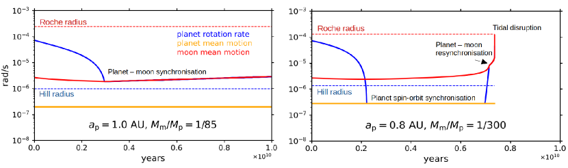
When we include the central star on the prize of neglecting the higher-order eccentricity terms and the obliquity parameter at all, we get to a differential equation system describing the time evolution of the rotation rates (stellar and planetary rotation), and the orbital frequencies (of the planet and the moon) which also describe the evolution of the orbital elements Sasaki et al. (2012). The behaviour of differential equation system also describes the tidal decay of the planetary rotation rate. This becomes important at the late stages of the planet–moon tidally locking (synchronization between the rotation of the planet and the mean motion of the moon); then the tidal decay of the planet’s rotation (both by forces from the star and from the moon) will reduce the planet’s rotation period to less than the moon’s orbital period. From this point, the tidal evolution of the moon’s semi-major axis reverts, and the moon starts gradually approaching the planet (left panel of Figure 2.
Needless to say that this is only possible if the moon does not escape for a long time, letting the planet’ rotation to slow down sufficiently. This is only possible for distant (warm and cold) planets, where the Hill radius is large, as we have already seen.
At this second, “approaching” evolution stage of the moon, an interesting feature was also been observed in simulations. The planet has initially two options to synchronize its rotation rate: it either synchronizes to the moon’s orbital rate (planet–moon locking), or to the planet’s orbital rate (planetary spin–orbit locking). This latter scenario is more possible if the moon has a lower mass and a more distant orbit, so the planet–star tidal interaction outperform the planet–moon tidal dynamics. In both cases, the moon starts approaching the planet from this point. When the moon gets close enough to the planet, the planet–moon tidal interactions will eventually supercede the star–planet interactions, when the planet’s rotation rate resynchronizes to the moon’s orbital rate. During this stage, a huge amount of energy dissipates and results in excess levels of tidal heating.
From this point, the disruption of the moon is unavoidable. The moon rapidly evolves to as close orbit as the Roche radius, being a catastrophic end of the body and spreading away in form of a dense ring around the planet. In some terminology this final stage is called as “collision to the planet”, which is a misleading term because collision does not happen at all, whereas the moon will be entirely exterminated.
The time scale of the tidal evolution is the most important key for an observable moon of a planet around an evolved star. In numerical experiments, simulating stochastically placed moon populations around all the known exoplanets by date, Dobos et al. (2021) concluded that in our currently known sample, only planets having an orbital period above 100-130 days have at least 50% chance for keeping a moon during 1 Gyr. This also confirms that the possible targets for “moon hunting” observation projects must include warm or cold, “normal” planets; while due to the signal-to-noise criterion of observations, the host star must be very bright. The shortage of the current exoplanet catalog in these possible targets and the further perspective for discovering a larger number of these will be discussed in Section 6.
5 The term for observability
5.1 Transiting exomoons
In the decades following the detection of the first extrasolar planet (Mayor and Queloz, 1995), the subfield of exoplanet science astronomy grew ever larger and more prominent in astronomy. This has led to the number of confirmed exoplanets surpassing 5000 in 2022111According to the NASA Exoplanet Archive, the number of known exoplanets is 5532 at the time of writing. A majority of these planets have been discovered by the so-called transit method, enabled by the use of space observatories such as Kepler (Borucki et al., 2010) and TESS (Ricker et al., 2015). The question of whether these planets can host a detectable moon arose almost naturally, following our knowledge of the Solar System. Several methods were put forward for the detection of exomoons. Most of these are applicable only when (at least) the host planet is found in a configuration leading to observable transits, including the direct modeling of planet plus moon transits (e.g. Szabó et al., 2006; Kipping, 2011), the analysis of Transit Timing Variations (of the host planet) (TTVs Simon et al., 2007; Kipping, 2009, 2009), or the Rossiter-McLaughlin effect Simon et al. (2010). Other methods, such as the detectability of radio emissions arising from the interaction between the moon and its host Noyola et al. (2014, 2016), direct imaging Kleisioti et al. (2023), and the thermal signatures of the moon Jäger and Szabó (2021) were also proposed.
Inspired by the success of the Mandel-Agol model (Mandel and Agol, 2002) used in the analysis of transit light curves of exoplanets, a number of models were proposed for the analysis of a planet–moon system, including: planetplanet (Luger et al., 2017; Kreidberg et al., 2019),
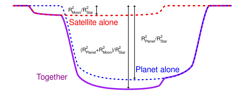
gefera (Gordon and Agol, 2022), Pandora (Hippke and Heller, 2022), the Photodynamic Agent of the Transit and Light Curve Modeler (TLCM, Csizmadia, 2020) (+ Kálmán et al, submitted), or the analytical model of Saha and Sengupta (2022) and the folding framework by Kipping (2021). Generally, these are based on two fully opaque, round bodies occulting a portion the stellar disk (Figure 2) or each other. Both the stability and the detectability terms have been taken into account in the “exomoon corridor” analysis by (Teachey, 2021) that can reveal dynamically stable moon with transit timing analysis, even considering muntiple-moon systems.
A full analytical formulation of transits and phase curves is published in Luger et al. (2022), which can handle spherical planets and moons, and also circular starspots; taken the mutual occultations (planet–moon, planet–starspot etc.) into account.
Heller et al. (2014) discusses the habitability of exomoons, in the light of their formation and observability, and concludes that natural satellites in the 0.1–0.5 R⊕ regime can be potentially habitable and observable. However, Szabó et al. (2011) and Simon et al. (2015) concludes that the detection limit for an exomoon in transit is roughly identical to that of the detectable planets, that is currently the size of Mars.
5.1.1 Proven false detections
At the time of writing, only a handful of exomoon candidates have been proposed. Dobos et al. (2022) compiled a potential target list for exomoon searches starting with all available planets to date, and found that the top 10 planets have more than 50% chance to be hosting a moon right now. Fox and Wiegert (2021) identified eight transiting exoplanets with TTVs in search of exomoons, while claiming that the observed signal in two of these systems is unlikely to have originated from an object orbiting the planet. Kipping (2020) suggested that the other six systems yield false positive signal as well. A dynamical analysis by Quarles et al. (2020) also implies that the KOIs-268.01, 303.01, 1888.01, 1925.01, 2728.01, 3320.01 could not host dynamically stable exomoons. Two perhaps more well-known examples of transiting exomoon candidates have also been put forward: Kepler-1625b-i (Teachey and Kipping, 2018) and Kepler-1708b-i (Kipping et al., 2022). Heller et al. (2019) provide an ‘alternative explanation’ for the observed signal in the former of these, suggesting that the combination of temporally correlated noise (in this case so-called ‘red noise’) and Bayesian inference can yield false positive detection. Kreidberg et al. (2019) show that by an independent extraction of the HST light curves of Teachey and Kipping (2018), light curve solutions without an exomoon are preferred. Both of these studies (Heller et al. 2019 and Kreidberg et al. 2019) suggest that the presence of red noise on the light curves can mimic a transit of an exomoon. As for the candidate exo-moon around the planet Kepler-1513 b, it has shown to be a false positive due to a second planet in the system Yahalomi et al. (2023).
The time-correlated noise can appear as a result of both instrumental and astrophysical noise sources, including pointing variations of the spacecraft, subpixel sensitivities, cosmis ray hits, stellar spots and oscillations, flares and microflares, granulation etc. The presence of these effects implies the need of a modeling tool with complex noise handling capabilities, such as the wavelet-formalism of Carter and Winn (2009), implemented into TLCM Csizmadia (2020). Rigorous testing of this algorithm suggests that it is effective in the removal of red noise from the light curves (Csizmadia et al., 2023), yielding stable parameters with correctly estimated uncertainties (Kálmán et al., 2023) for light curves of exoplanets. It is expected that the Photodynamic Agent update (Kálmán et al, in press) will also have similar success in the analysis of the transits of planet–moon systems. Furthermore, in Kálmán et al (in press) we also suggest that synthetic correlated nose models can quite easily mimic the transits of an exomoon, thus drawing attention to the possiblity of false positive detections. The tidal interactions can help the detection in the infrared by heating up the moon, even if the companion belongs to an otherwise cold planet, far from the host star (Jäger and Szabó, 2021).
5.2 Other detection methods than transit
In the followings we are summarizing the detection methods suggested for detecting a moon, besides the transit spectroscopy. While the baseline method remained the transit photometry, these alternative methods can be considered as possible ways to discovery with a specific instrument (e.g. when only spectroscopy is observed with a high performance space telescope), or independent opportunities to confirm a previously claimed detectionm using e.g. transit photometry.
5.2.1 Radial velocity of the parent planet
The extra radial velocity of a planet orbiting its parent star, induced by the gravitational perturbation by a moon, is given by
| (7) |
For instance, for a 1 Earth planet mass moon orbiting a 0.3 Saturn mass planet at au from the planet, the radial velocity wobble of the latter will be K = 1 km/sec, detectable with a ELT class telescope.
5.2.2 Rossitter-McLaughlin effect due to a moon
It has been suggested that moons around transiting exoplanets may cause an observable signal in the Rossiter-McLaughlin (RM) effect. In Simon et al. (2010), the possibility of the parameter reconstruction is demonstrated from the moon’s RM effect in a large variety of planet-moon configurations. The generic parameter space is of 20 dimensions with several degeneracies. The most promising parameter to reconstruct is the size of the moon, abd in some cases, there is also meaningful information on its orbital period. The angles of the orbital plane of the moon can only be derived if the transit time of the moon is exactly known, e.g. from earlier transit photometry.
5.2.3 Astrometry of the parent planet
The maximum angular deviation of a planet orbiting its parent star is given by
| (8) |
For a 1 Earth mass moon at 1 million km of a 0.1 Saturn mass planet at 5 pc, the maximum angular deviation is 0.3 mas. With a 8 m space telescope, the planet image at 400 nm is 10 mas wide. A Jupiter-sized planet at 1 au from a solar-type star at 5 pc gives, with a 30 m diameter telescope, N = photons reflected from the star in a 1 hour exposure in a 300 nm band. The astrometric precision on its position is then 10 mas / = 0.2 mas, sufficient to detect amplitude of the planet wobble due to the moon revolution.
5.2.4 Planet-moon mutual events
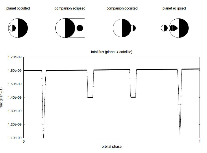
On average, in a direct image of the parent planet reflecting the parent star light, the moon reflects also the star light. But, for some parts of its orbit around the planet, it may partially mask the planet, either by transiting it or by projecting its shadow on the illuminated part of the planet. The moon is also totally eclipsed during a part of its revolution around the planet Figure 3 shows the resulting light curve of the planet + moon system reflecting the parent star.
5.2.5 Microlensing
When a background star passes through the Einstein radius of a foreground star, we can observe an excess peak on the light curve. The Einstein-radius is defined as:
| (9) |
When the foreground star has a planetary companion, there is a secondary peak created by the planet. When the planet itself has a moon, the background star light curve becomes mire complicated, revealing the presence of the moon, as has been suspected for OGLE-2015-BLG-1459L Hwang et al. (2018).
5.2.6 Direct detection
Extremely large ground based telescopes will reach a contrast, sufficient to detect an earth-sized planet. With diameters larger than 30 m they will have an angular resolution of 2.5 mas, sufficient to detect an Earth-sized moon at 0.01 au from a planet at 5 pc.
5.2.7 Transit spectroscopy of the exo-moon atmosphere
Transmission spectroscopy with JWST should be able to detect molecular species for the spectral retrieval of molecules in their atmosphere Kipping et al. (2010).
6 Discussion
6.1 The structure of the question
The “real” Drake-equation has a structure where the earlier terms are known better or can be better approximated, while the terms at the end are merely still unknown. Unlike this, the exomoon cascade equation has the opposite structure. The detection term at the end of the equation is the most tangible, because we see the instruments for the detection, even detailed tests can be extensively assessed. The first term, the formation is rather the most abstract in our cascade equation, because we have not seen an exomoon in formation (note here the possible exceptional case of PS70, Benisty et al. (2021)); while the orbital evolution of the moons can also be experienced via indirect observations, mostly the moon structures in our Solar System. The different methodological difficulties are seen in the timeline of the publications about the different aspects.
| Subfiled | Number of Papers | Number of Citatons | H-index | Tori-index |
|---|---|---|---|---|
| Formation | 180 | 5198 | 36 | 27.7 |
| Stability | 114 | 2461 | 27 | 21.5 |
| Detection | 384 | 11993 | 54 | 65.9 |
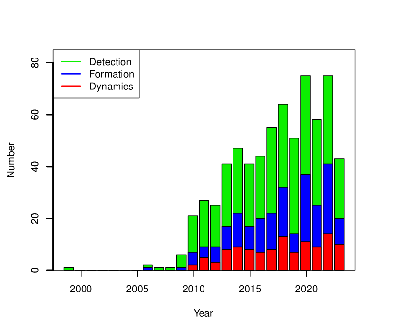
By now, all the the three fields of exomoon formation, orbital evolution and observability have been discussed in many publications, which are summarized in Table 2 and graphically shown in Figure 4. The earliest and the most widely studied question has been the observation. Here publications cover the theory of observations (suggested methods and data analysis tools; many of these papers have been mentioned in this review); and also feasibility studies, where injections are added to simulated observations with realistic noise (white and often correlated noise parts as well), sampling, gaps, outlier points etc., and they are finding the injection with blind solutions. The post-solution comparison of the best fit parameters to the injection parameters return with the reliability of the parameters and this process can determine the detection threshold, with the aim to guarantee that most alerts in actual observation will represent a true positive moon detection in fact. These studies are highly driven by the development of new instruments and the always renewing research programs that dedicate more and more efforts to exomoon search in the most appropriate approach.
The moon formation studies and the dynamics are usually studied in relation to the formation of solar systems in general, in interpreting the moon formation in our Solar System, or in respect to the search for habitable worlds. It has been discussed in this paper earlier how extremely multi-layered problem this is, often facing the research to challenges in the physical complexity of the appropriate models, and practical computation limits as well. These two fields together have about similar number of publications than the observation aspects. The study of these fields started a couple of years later than the observability studies, but after revealing the actual physical processes behind a moon, the results propagated efficiently in the community and the naive assumptions about exomoons disappeared from the data analysis works as well. (For example, no one hopes to find exomoons around hot Jupiters any more, hence no upper limits are derived for these, etc.)
6.2 The insufficiency of the catalogs
| Host star | No. planets d | Period [d] | G mag | Discovery |
|---|---|---|---|---|
| HD 136352 | 1 | 107.245 | 5.485 | Delrez et al. (2021) (2021) |
| GJ 414 A | 1 | 749.83 | 7.720 | Dedrick et al. (2021) (2021) |
| HD 114082 | 1 | 109.75 | 8.094 | Zakhozhay et al. (2022) (2022) |
| HIP 41378 | 3 | 278, 369, 542 † | 8.810 | Vanderburg et al. (2016) (2016) |
| HD 80606 | 1 | 111.436 | 8.820 | Pont et al. (2009) (2009) |
| TOI-2180 b | 1 | 260.79 | 9.011 | Dalba et al. (2022) (2022) |
| TIC 172900988 A | 1 | 188-204 ‡ | 10.048 | Kostov et al. (2021) (2021) |
| Kepler-126 | 1 | 100.283 | 10.454 | Rowe et al. (2014) (2014) |
| TOI-199 | 1 | 104.854 | 10.578 | Hobson et al. (2023) (2023) |
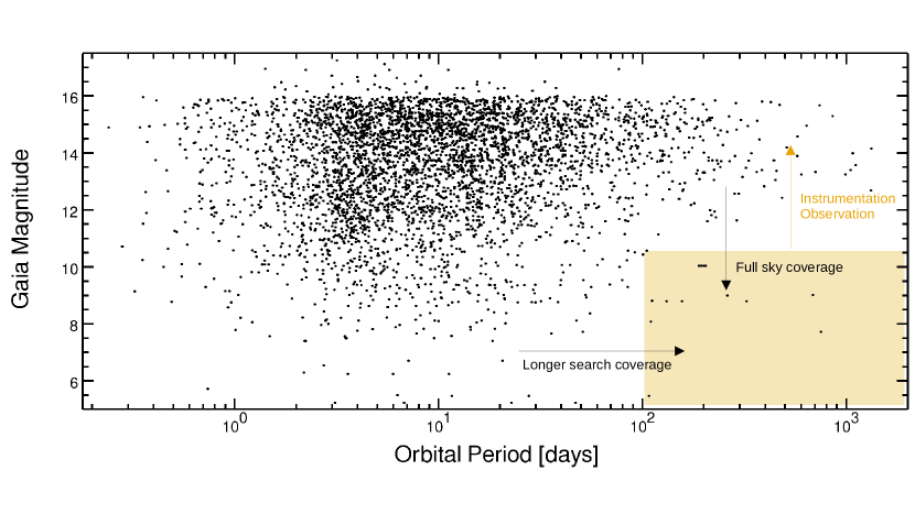
Due to the dynamical constraints, the exoplanet hosting stars can be characterized by day orbital period, and the longer the period the more chance an exomoon has to be on stable orbit. Also, the signal-to-noise criterion is very demanding when trying to detect the exomoons, because any photometric signal is inversely scaled by the 2nd power of the radius of the exomoon (proportional to the area of the moon’s disk in sky projection, much compressing the signal we wish to detect. Even so, any dynamical effect, e.g. transit timing variation is inversely scaled by the 3rd power of the relative radius (via the mass ratio). The resulting low signal levels demands extreme precision which is best suited by spaceborn instruments. Taking the actual performance into account, a reasonable limit of 10–11 magnitude can be considered for meter-category space telescopes, and the JWST may by efficient down to 13 magnitude.
Taken these constraints in mind, an “exomoon search region” can be defined as d, mag. Despite the more than 5500 confirmed exoplanets so far, we still have insufficient number of planets in the exmoon search region. Figure 5 shows the distribution of the confirmed exoplanets in the period–magnirude space, having the search region overplotted. There are a few planets within the region which is summarized in Table 3. Somewhat surprisingly, the number of promising targets in our search area has increased very significantly in the past few years, 6 of 9 systems were discovered in 2021 or later. This rapidly increasing rate of discoveries can be devoted to the long observation time basis for planet search (e.g. repeated TESS visits) and the evolution of the observation strategies (e.g. follow-up long-period TESS planet candidates to determine the accurate period, (e.g. Delrez et al., 2021; Ulmer-Moll et al., 2023; Garai et al., 2023; Osborn et al., 2023)), which help the precise characterisation of the long-period transiting planets. The chance of getting more and more appropriate candidates within the exomoon search region due to the longer time coverage of observations and also, better resolution of the full sky with the appropriately long and precise observations (as indicated by the arrows in Figure 5.
Most of the current and future space observatories have an exomoon program. The JWST is capable to detect super-Titans around isolated planetary-mass objects Limbach et al. (2021, 2022), and when the homogeneous surface temperature distribution is taken into account, Titan category exomoons can also be considered Jäger and Szabó (2021). CHEOPS Benz et al. (2021) has also attempted detecting large exomoons around long-period planets the large exomoons Ehrenreich et al. (2023), PLATO will be searching for exomoons from transit photometry Rauer et al. (2014), while Ariel will also have a program to detect exomoons and rings using the photometers in the optical and synthetic spectrophotometry in the infrared. Szabó et al. (2022).
6.3 Open questions
The exomoon studies had seen an intense development in the past years, and by now, the field has a long frontline that progresses into the unknown. The open questions addressed here are by no means considered to be comprehensive, rather they are selected aspects of the “exomoon chase” efforts which the authors consider to be especially important, and the role of this list is to propose further directions of research for the interested expert. The structure follows the formation – dynamics – observation arrangement.
-
1.
Formation
A central question concerning formation is how large exomoons we can hope to observe. Is there upper limit for a moon in mass or size? What is the best target we are hunting for?
What is the occurrence of moons around different types of planets, and what is the size dependence of the occurrence? Does the exomoon occurrence in general have some spatial dependence in the well observable parts of the Galaxy?
Are there observable diagnostics or proxy parameters belonging to an exomoon? Are there some special stellar and/or planetary parameters that, at least in a combination, can serve as a red light for a large exomoon? Understanding these aspects are just conceptual for the observation work.
Also, the validity of different formation pathways for moons is a debated question. Which of the suggested processes is acting in real systems, and what is the parameter preference of the different modes? There is still many aspects to understand about the possible formation ways of the Solar System moons as well.
-
2.
Dynamics
How well the current equations describe the orbital evolution of the moons? Tidal dynamics is a very complex process in itself, while in real systems, this will be embedded in the N-body problem of a whole solar system. Are we still missing some key aspect that can rearrange the entire picture of our current understanding here?
The tidal heating itself also has a wide horizon on the habitability studies and the search for the life-supporting environment. Here the key question is the actual eccentricity of the systems, the initial distribution of the eccentricity and the time scale and precision of the circularization processes.
-
3.
Observations
From the technical aspect, high-level signal reconstruction is required. Here the adaptive handling of possible known sources of systematics, such as data from telemetry and imaging and the less predictable sources like stellar noise is a central question that can help get rid of the several (very probably) false positive detections that have been already advertised. (Here we can remark that at the early stages of exoplanet discovery, there were also a meaningful number of false positives, representing inherent characteristic of very difficult observations.)
An open question for observations is that after the first discovered exomoons, how can we learn something about the internal structure of exomoons. Atmospheric spectroscopy and thermal photometry are two suggested pathways for the future to reveal the reality of these still unknown worlds.
One of the most exciting possibility is the imaging of exomoons. is a reasonable hope with future ground-based (like the E-ELT) or lunar very big instruments. For instance, 1) a 10x10 pixel image of an icy exo-moon with a lunar hypertelescope (Labeyrie et al. 2020 Lunar or space-based hypertelescope for direct high-resolution imaging Labeyrie et al. (2021) will reveal plumes, like for Europa 2) if the surface of the exo-moon is inhomogeneous, multiple subsequent images will tell if the moon is co-rotating with its parent planet (like our Moon); that will give another information of the moon internal structure.
7 Concluding remarks
In 2024, the study of exomoons Sartoretti and Schneider (1999) is seeing its 25th anniversary. During the phe past quater century, the true astrophysical and observational complexity of the task, and the actual impediments on the way to the first confirmed detection. The following years are very promising in this sense, because we are just in the position of discovering a favourable amount of long period planets around enough bright stars. By following the prediction methodology of 2019arXiv191112114H who predict 100,000 exoplanets by 2050, there is a reasonable hope to have many thousands of long-period planets that can host a moon physically; and if the detection rate will be in the order of a few percents, we can expect dozens, or maybe hundreds of confirmed exomoons by the 50th anniversary of the field.
Conceptualisation, writing, editing and publishing: Gy. M. Sz. General consulting, Sect. 5.2, 6.5 (3), Sect 1 paragraph 1: J. Sch. Structural idea and literature review for Sections 3 and 4: D. Z. Full elaboration of 5.1.: Sz. K.
SzK and GyMSz thank the PRODEX Experiment Agreement No. 4000137122 between the ELTE Eötvös Loránd University and the European Space Agency (ESA-D/SCI-LE-2021-0025). Project no. C1746651 has been implemented with the support provided by the Ministry of Culture and Innovation of Hungary from the National Research, Development and Innovation Fund, financed under the NVKDP-2021 funding scheme.
No new data is generated in relation to this study.
Acknowledgements.
Jean Schneider is grateful to Juan Cabrera for the Figure 2 \conflictsofinterestThe authors declare no conflict of interest. \abbreviationsAbbreviations The following abbreviations are used in this manuscript:\reftitleReferences \externalbibliographyyes
References
- Mayor and Queloz (1995) Mayor, M.; Queloz, D. A Jupiter-mass companion to a solar-type star. Nature 1995, 378, 355–359. https://doi.org/10.1038/378355a0.
- Charbonneau et al. (2002) Charbonneau, D.; Brown, T.M.; Noyes, R.W.; Gilliland, R.L. Detection of an Extrasolar Planet Atmosphere. ApJ 2002, 568, 377–384, [arXiv:astro-ph/astro-ph/0111544]. https://doi.org/10.1086/338770.
- Moutou et al. (2013) Moutou, C.; Deleuil, M.; Guillot, T.; Baglin, A.; Bordé, P.; Bouchy, F.; Cabrera, J.; Csizmadia, S.; Deeg, H.J. CoRoT: Harvest of the exoplanet program. Icarus 2013, 226, 1625–1634, [arXiv:astro-ph.EP/1306.0578]. https://doi.org/10.1016/j.icarus.2013.03.022.
- Mullally et al. (2015) Mullally, F.; Coughlin, J.L.; Thompson, S.E.; Rowe, J.; Burke, C.; Latham, D.W.; Batalha, N.M.; Bryson, S.T.; Christiansen, J.; Henze, C.E.; et al. Planetary Candidates Observed by Kepler. VI. Planet Sample from Q1–Q16 (47 Months). ApJS 2015, 217, 31, [arXiv:astro-ph.EP/1502.02038]. https://doi.org/10.1088/0067-0049/217/2/31.
- Ricker et al. (2015) Ricker, G.R.; Winn, J.N.; Vanderspek, R.; Latham, D.W.; Bakos, G.Á.; Bean, J.L.; Berta-Thompson, Z.K.; Brown, T.M.; Buchhave, L.; Butler, N.R.; et al. Transiting Exoplanet Survey Satellite (TESS). Journal of Astronomical Telescopes, Instruments, and Systems 2015, 1, 014003. https://doi.org/10.1117/1.JATIS.1.1.014003.
- Benz et al. (2021) Benz, W.; Broeg, C.; Fortier, A.; Rando, N.; Beck, T.; Beck, M.; Queloz, D.; Ehrenreich, D.; Maxted, P.F.L.; Isaak, K.G.; et al. The CHEOPS mission. Experimental Astronomy 2021, 51, 109–151, [arXiv:astro-ph.IM/2009.11633]. https://doi.org/10.1007/s10686-020-09679-4.
- Sartoretti and Schneider (1999) Sartoretti, P.; Schneider, J. On the detection of satellites of extrasolar planets with the method of transits. A&AS 1999, 134, 553–560. https://doi.org/10.1051/aas:1999148.
- Szabó et al. (2006) Szabó, G.M.; Szatmáry, K.; Divéki, Z.; Simon, A. Possibility of a photometric detection of “exomoons”. A&A 2006, 450, 395–398, [arXiv:astro-ph/astro-ph/0601186]. https://doi.org/10.1051/0004-6361:20054555.
- Simon et al. (2007) Simon, A.; Szatmáry, K.; Szabó, G.M. Determination of the size, mass, and density of “exomoons” from photometric transit timing variations. A&A 2007, 470, 727–731, [arXiv:astro-ph/0705.1046]. https://doi.org/10.1051/0004-6361:20066560.
- Kipping (2009) Kipping, D.M. Transit timing effects due to an exomoon. MNRAS 2009, 392, 181–189, [arXiv:astro-ph/0810.2243]. https://doi.org/10.1111/j.1365-2966.2008.13999.x.
- Ogilvie and Lin (2004) Ogilvie, G.I.; Lin, D.N.C. Tidal Dissipation in Rotating Giant Planets. ApJ 2004, 610, 477–509, [arXiv:astro-ph/astro-ph/0310218]. https://doi.org/10.1086/421454.
- Alvarado-Montes et al. (2017) Alvarado-Montes, J.A.; Zuluaga, J.I.; Sucerquia, M. The effect of close-in giant planets’ evolution on tidal-induced migration of exomoons. MNRAS 2017, 471, 3019–3027, [arXiv:astro-ph.EP/1707.02906]. https://doi.org/10.1093/mnras/stx1745.
- Dobos et al. (2021) Dobos, V.; Charnoz, S.; Pál, A.; Roque-Bernard, A.; Szabó, G.M. Survival of Exomoons Around Exoplanets. PASP 2021, 133, 094401, [arXiv:astro-ph.EP/2105.12040]. https://doi.org/10.1088/1538-3873/abfe04.
- Tokadjian and Piro (2023) Tokadjian, A.; Piro, A.L. Tidal Heating of Exomoons in Resonance and Implications for Detection. AJ 2023, 165, 173, [arXiv:astro-ph.EP/2206.11368]. https://doi.org/10.3847/1538-3881/acc254.
- Schneider et al. (2015) Schneider, J.; Lainey, V.; Cabrera, J. A next step in exoplanetology: exo-moons. International Journal of Astrobiology 2015, 14, 191–199. https://doi.org/10.1017/S1473550414000299.
- Muirhead et al. (2012) Muirhead, P.S.; Johnson, J.A.; Apps, K.; Carter, J.A.; Morton, T.D.; Fabrycky, D.C.; Pineda, J.S.; Bottom, M.; Rojas-Ayala, B.; Schlawin, E.; et al. Characterizing the Cool KOIs. III. KOI 961: A Small Star with Large Proper Motion and Three Small Planets. ApJ 2012, 747, 144, [arXiv:astro-ph.SR/1201.2189]. https://doi.org/10.1088/0004-637X/747/2/144.
- Malamud et al. (2020) Malamud, U.; Perets, H.B.; Schäfer, C.; Burger, C. Collisional formation of massive exomoons of superterrestrial exoplanets. MNRAS 2020, 492, 5089–5101, [arXiv:astro-ph.EP/1904.12854]. https://doi.org/10.1093/mnras/staa211.
- Cabrera and Schneider (2007) Cabrera, J.; Schneider, J. Detecting companions to extrasolar planets using mutual events. A&A 2007, 464, 1133–1138, [arXiv:astro-ph/astro-ph/0703609]. https://doi.org/10.1051/0004-6361:20066111.
- Roccetti et al. (2023) Roccetti, G.; Grassi, T.; Ercolano, B.; Molaverdikhani, K.; Crida, A.; Braun, D.; Chiavassa, A. Presence of liquid water during the evolution of exomoons orbiting ejected free-floating planets. International Journal of Astrobiology 2023, 22, 317–346, [arXiv:astro-ph.EP/2302.04946]. https://doi.org/10.1017/S1473550423000046.
- Sajadian and Sangtarash (2023) Sajadian, S.; Sangtarash, P. Microlensing due to free-floating moon-planet systems. MNRAS 2023, 520, 5613–5621, [arXiv:astro-ph.EP/2302.05230]. https://doi.org/10.1093/mnras/stad484.
- Drake (1961) Drake, F.D. Project Ozma. Physics Today 1961, 14, 40. https://doi.org/10.1063/1.3057500.
- Simon et al. (2010) Simon, A.E.; Szabó, G.M.; Szatmáry, K.; Kiss, L.L. Methods for exomoon characterization: combining transit photometry and the Rossiter-McLaughlin effect. MNRAS 2010, 406, 2038–2046, [arXiv:astro-ph.SR/1004.1143]. https://doi.org/10.1111/j.1365-2966.2010.16818.x.
- Sasaki et al. (2012) Sasaki, T.; Barnes, J.W.; O’Brien, D.P. Outcomes and Duration of Tidal Evolution in a Star-Planet-Moon System. ApJ 2012, 754, 51, [arXiv:astro-ph.EP/1206.0334]. https://doi.org/10.1088/0004-637X/754/1/51.
- Heller and Barnes (2013) Heller, R.; Barnes, R. Exomoon Habitability Constrained by Illumination and Tidal Heating. Astrobiology 2013, 13, 18–46, [arXiv:astro-ph.EP/1209.5323]. https://doi.org/10.1089/ast.2012.0859.
- Heller et al. (2014) Heller, R.; Williams, D.; Kipping, D.; Limbach, M.A.; Turner, E.; Greenberg, R.; Sasaki, T.; Bolmont, É.; Grasset, O.; Lewis, K.; et al. Formation, Habitability, and Detection of Extrasolar Moons. Astrobiology 2014, 14, 798–835, [arXiv:astro-ph.EP/1408.6164]. https://doi.org/10.1089/ast.2014.1147.
- Mosqueira and Estrada (2003) Mosqueira, I.; Estrada, P.R. Formation of the regular satellites of giant planets in an extended gaseous nebula I: subnebula model and accretion of satellites. Icarus 2003, 163, 198–231. https://doi.org/10.1016/S0019-1035(03)00076-9.
- Estrada et al. (2009) Estrada, P.R.; Mosqueira, I.; Lissauer, J.J.; D’Angelo, G.; Cruikshank, D.P. Formation of Jupiter and Conditions for Accretion of the Galilean Satellites. In Europa; Pappalardo, R.T.; McKinnon, W.B.; Khurana, K.K., Eds.; 2009; p. 27. https://doi.org/10.48550/arXiv.0809.1418.
- Heller and Pudritz (2015a) Heller, R.; Pudritz, R. Water Ice Lines and the Formation of Giant Moons around Super-Jovian Planets. ApJ 2015, 806, 181, [arXiv:astro-ph.EP/1410.5802]. https://doi.org/10.1088/0004-637X/806/2/181.
- Heller and Pudritz (2015b) Heller, R.; Pudritz, R. Conditions for water ice lines and Mars-mass exomoons around accreting super-Jovian planets at 1-20 AU from Sun-like stars. A&A 2015, 578, A19, [arXiv:astro-ph.EP/1504.01668]. https://doi.org/10.1051/0004-6361/201425487.
- Canup and Ward (2006) Canup, R.M.; Ward, W.R. A common mass scaling for satellite systems of gaseous planets. Nature 2006, 441, 834–839. https://doi.org/10.1038/nature04860.
- Canup and Ward (2009) Canup, R.M.; Ward, W.R. Origin of Europa and the Galilean Satellites. In Europa; Pappalardo, R.T.; McKinnon, W.B.; Khurana, K.K., Eds.; 2009; p. 59. https://doi.org/10.48550/arXiv.0812.4995.
- Sasaki et al. (2010) Sasaki, T.; Stewart, G.R.; Ida, S. Origin of the Different Architectures of the Jovian and Saturnian Satellite Systems. ApJ 2010, 714, 1052–1064, [arXiv:astro-ph.EP/1003.5737]. https://doi.org/10.1088/0004-637X/714/2/1052.
- Heller (2020) Heller, R. Astrophysical Simulations and Data Analyses on the Formation, Detection, and Habitability of Moons Around Extrasolar Planets. arXiv e-prints 2020, p. arXiv:2009.01881, [arXiv:astro-ph.EP/2009.01881]. https://doi.org/10.48550/arXiv.2009.01881.
- Crida and Charnoz (2012) Crida, A.; Charnoz, S. Formation of Regular Satellites from Ancient Massive Rings in the Solar System. Science 2012, 338, 1196, [arXiv:astro-ph.EP/1301.3808]. https://doi.org/10.1126/science.1226477.
- Canup and Asphaug (2001) Canup, R.M.; Asphaug, E. Origin of the Moon in a giant impact near the end of the Earth’s formation. Nature 2001, 412, 708–712.
- Canup (2004) Canup, R.M. Simulations of a late lunar-forming impact. Icarus 2004, 168, 433–456. https://doi.org/10.1016/j.icarus.2003.09.028.
- Hyodo et al. (2015) Hyodo, R.; Ohtsuki, K.; Takeda, T. Formation of Multiple-satellite Systems From Low-mass Circumplanetary Particle Disks. ApJ 2015, 799, 40, [arXiv:astro-ph.EP/1411.4336]. https://doi.org/10.1088/0004-637X/799/1/40.
- Kokubo and Genda (2010) Kokubo, E.; Genda, H. Formation of Terrestrial Planets from Protoplanets Under a Realistic Accretion Condition. ApJ 2010, 714, L21–L25, [arXiv:astro-ph.EP/1003.4384]. https://doi.org/10.1088/2041-8205/714/1/L21.
- Charnoz (2009) Charnoz, S. Physical collisions of moonlets and clumps with the Saturn’s F-ring core. Icarus 2009, 201, 191–197, [arXiv:astro-ph.EP/0901.0482]. https://doi.org/10.1016/j.icarus.2008.12.036.
- Canup (2012) Canup, R.M. Forming a Moon with an Earth-like Composition via a Giant Impact. Science 2012, 338, 1052. https://doi.org/10.1126/science.1226073.
- Debes and Sigurdsson (2007) Debes, J.H.; Sigurdsson, S. The Survival Rate of Ejected Terrestrial Planets with Moons. ApJ 2007, 668, L167–L170, [arXiv:astro-ph/0709.0945]. https://doi.org/10.1086/523103.
- Morbidelli et al. (2012) Morbidelli, A.; Tsiganis, K.; Batygin, K.; Crida, A.; Gomes, R. Explaining why the uranian satellites have equatorial prograde orbits despite the large planetary obliquity. Icarus 2012, 219, 737–740, [arXiv:astro-ph.EP/1208.4685]. https://doi.org/10.1016/j.icarus.2012.03.025.
- Szulágyi et al. (2018) Szulágyi, J.; Cilibrasi, M.; Mayer, L. In Situ Formation of Icy Moons of Uranus and Neptune. ApJ 2018, 868, L13, [arXiv:astro-ph.EP/1811.06574]. https://doi.org/10.3847/2041-8213/aaeed6.
- Astakhov et al. (2003) Astakhov, S.A.; Burbanks, A.D.; Wiggins, S.; Farrelly, D. Chaos-assisted capture of irregular moons. Nature 2003, 423, 264–267. https://doi.org/10.1038/nature01622.
- Williams (2013) Williams, D.M. Capture of Terrestrial-Sized Moons by Gas Giant Planets. Astrobiology 2013, 13, 315–323. https://doi.org/10.1089/ast.2012.0892.
- Agnor and Hamilton (2006) Agnor, C.B.; Hamilton, D.P. Neptune’s capture of its moon Triton in a binary-planet gravitational encounter. Nature 2006, 441, 192–194. https://doi.org/10.1038/nature04792.
- Heller (2018) Heller, R. The nature of the giant exomoon candidate Kepler-1625 b-i. A&A 2018, 610, A39, [arXiv:astro-ph.EP/1710.06209]. https://doi.org/10.1051/0004-6361/201731760.
- Chandrasekhar (1963) Chandrasekhar, S. The Equilibrium and the Stability of the Roche Ellipsoids. ApJ 1963, 138, 1182. https://doi.org/10.1086/147716.
- Hamilton and Burns (1992) Hamilton, D.P.; Burns, J.A. Orbital stability zones about asteroids II. The destabilizing effects of eccentric orbits and of solar radiation. Icarus 1992, 96, 43–64. https://doi.org/10.1016/0019-1035(92)90005-R.
- Holman and Wiegert (1999) Holman, M.J.; Wiegert, P.A. Long-Term Stability of Planets in Binary Systems. AJ 1999, 117, 621–628, [arXiv:astro-ph/astro-ph/9809315]. https://doi.org/10.1086/300695.
- Barnes and O’Brien (2002) Barnes, J.W.; O’Brien, D.P. Stability of Satellites around Close-in Extrasolar Giant Planets. ApJ 2002, 575, 1087–1093, [arXiv:astro-ph/astro-ph/0205035]. https://doi.org/10.1086/341477.
- Domingos et al. (2006) Domingos, R.C.; Winter, O.C.; Yokoyama, T. Stable satellites around extrasolar giant planets. MNRAS 2006, 373, 1227–1234. https://doi.org/10.1111/j.1365-2966.2006.11104.x.
- Heller et al. (2011) Heller, R.; Leconte, J.; Barnes, R. Tidal obliquity evolution of potentially habitable planets. A&A 2011, 528, A27, [arXiv:astro-ph.EP/1101.2156]. https://doi.org/10.1051/0004-6361/201015809.
- Borucki et al. (2010) Borucki, W.J.; Koch, D.; Basri, G.; Batalha, N.; Brown, T.; Caldwell, D.; Caldwell, J.; Christensen-Dalsgaard, J.; Cochran, W.D.; DeVore, E.; et al. Kepler Planet-Detection Mission: Introduction and First Results. Science 2010, 327, 977. https://doi.org/10.1126/science.1185402.
- Kipping (2011) Kipping, D.M. LUNA: A Transit Algorithm for Exomoons. In Proceedings of the AAS/Division for Extreme Solar Systems Abstracts, 2011, Vol. 2, AAS/Division for Extreme Solar Systems Abstracts, p. 19.02.
- Kipping (2009) Kipping, D.M. Transit timing effects due to an exomoon - II. MNRAS 2009, 396, 1797–1804, [arXiv:astro-ph.EP/0904.2565]. https://doi.org/10.1111/j.1365-2966.2009.14869.x.
- Noyola et al. (2014) Noyola, J.P.; Satyal, S.; Musielak, Z.E. Detection of Exomoons through Observation of Radio Emissions. ApJ 2014, 791, 25, [arXiv:astro-ph.EP/1308.4184]. https://doi.org/10.1088/0004-637X/791/1/25.
- Noyola et al. (2016) Noyola, J.P.; Satyal, S.; Musielak, Z.E. On the Radio Detection of Multiple-exomoon Systems due to Plasma Torus Sharing. ApJ 2016, 821, 97, [arXiv:astro-ph.EP/1603.01862]. https://doi.org/10.3847/0004-637X/821/2/97.
- Kleisioti et al. (2023) Kleisioti, E.; Dirkx, D.; Rovira-Navarro, M.; Kenworthy, M.A. Tidally heated exomoons around Eridani b: Observability and prospects for characterization. A&A 2023, 675, A57, [arXiv:astro-ph.EP/2305.03410]. https://doi.org/10.1051/0004-6361/202346082.
- Jäger and Szabó (2021) Jäger, Z.; Szabó, G.M. Enhanced thermal radiation from a tidally heated exomoon with a single hotspot. MNRAS 2021, 508, 5524–5537, [arXiv:astro-ph.EP/2110.05353]. https://doi.org/10.1093/mnras/stab2955.
- Mandel and Agol (2002) Mandel, K.; Agol, E. Analytic Light Curves for Planetary Transit Searches. ApJ 2002, 580, L171–L175, [arXiv:astro-ph/astro-ph/0210099]. https://doi.org/10.1086/345520.
- Luger et al. (2017) Luger, R.; Lustig-Yaeger, J.; Agol, E. Planet-Planet Occultations in TRAPPIST-1 and Other Exoplanet Systems. ApJ 2017, 851, 94, [arXiv:astro-ph.EP/1711.05739]. https://doi.org/10.3847/1538-4357/aa9c43.
- Kreidberg et al. (2019) Kreidberg, L.; Luger, R.; Bedell, M. No Evidence for Lunar Transit in New Analysis of Hubble Space Telescope Observations of the Kepler-1625 System. ApJ 2019, 877, L15, [arXiv:astro-ph.EP/1904.10618]. https://doi.org/10.3847/2041-8213/ab20c8.
- Gordon and Agol (2022) Gordon, T.A.; Agol, E. Analytic Light Curve for Mutual Transits of Two Bodies Across a Limb-darkened Star. AJ 2022, 164, 111, [arXiv:astro-ph.EP/2207.06024]. https://doi.org/10.3847/1538-3881/ac82b1.
- Hippke and Heller (2022) Hippke, M.; Heller, R. Pandora: A fast open-source exomoon transit detection algorithm. A&A 2022, 662, A37, [arXiv:astro-ph.EP/2205.09410]. https://doi.org/10.1051/0004-6361/202243129.
- Csizmadia (2020) Csizmadia, S. The Transit and Light Curve Modeller. MNRAS 2020, 496, 4442–4467. https://doi.org/10.1093/mnras/staa349.
- Saha and Sengupta (2022) Saha, S.; Sengupta, S. Transit Light Curves for Exomoons: Analytical Formalism. ApJ 2022, 936, 2, [arXiv:astro-ph.EP/2203.10881]. https://doi.org/10.3847/1538-4357/ac85a9.
- Kipping (2021) Kipping, D. Transit origami: a method to coherently fold exomoon transits in time series photometry. MNRAS 2021, 507, 4120–4131, [arXiv:astro-ph.EP/2108.02903]. https://doi.org/10.1093/mnras/stab2013.
- Teachey (2021) Teachey, A. The exomoon corridor for multiple moon systems. MNRAS 2021, 506, 2104–2121, [arXiv:astro-ph.EP/2106.13421]. https://doi.org/10.1093/mnras/stab1840.
- Luger et al. (2022) Luger, R.; Agol, E.; Bartolić, F.; Foreman-Mackey, D. Analytic Light Curves in Reflected Light: Phase Curves, Occultations, and Non-Lambertian Scattering for Spherical Planets and Moons. AJ 2022, 164, 4, [arXiv:astro-ph.EP/2103.06275]. https://doi.org/10.3847/1538-3881/ac4017.
- Szabó et al. (2011) Szabó, G.M.; Simon, A.E.; Kiss, L.L.; Regály, Z. Practical suggestions on detecting exomoons in exoplanet transit light curves. In Proceedings of the The Astrophysics of Planetary Systems: Formation, Structure, and Dynamical Evolution; Sozzetti, A.; Lattanzi, M.G.; Boss, A.P., Eds., 2011, Vol. 276, pp. 556–557, [arXiv:astro-ph.SR/1012.1560]. https://doi.org/10.1017/S174392131102120X.
- Simon et al. (2015) Simon, A.E.; Szabó, G.M.; Kiss, L.L.; Fortier, A.; Benz, W. CHEOPS Performance for Exomoons: The Detectability of Exomoons by Using Optimal Decision Algorithm. PASP 2015, 127, 1084, [arXiv:astro-ph.EP/1508.00321]. https://doi.org/10.1086/683392.
- Dobos et al. (2022) Dobos, V.; Haris, A.; Kamp, I.E.E.; van der Tak, F.F.S. A target list for searching for habitable exomoons. MNRAS 2022, 513, 5290–5298, [arXiv:astro-ph.EP/2204.11614]. https://doi.org/10.1093/mnras/stac1180.
- Fox and Wiegert (2021) Fox, C.; Wiegert, P. Exomoon candidates from transit timing variations: eight Kepler systems with TTVs explainable by photometrically unseen exomoons. MNRAS 2021, 501, 2378–2393, [arXiv:astro-ph.EP/2006.12997]. https://doi.org/10.1093/mnras/staa3743.
- Kipping (2020) Kipping, D. An Independent Analysis of the Six Recently Claimed Exomoon Candidates. ApJ 2020, 900, L44, [arXiv:astro-ph.EP/2008.03613]. https://doi.org/10.3847/2041-8213/abafa9.
- Quarles et al. (2020) Quarles, B.; Li, G.; Rosario-Franco, M. Application of Orbital Stability and Tidal Migration Constraints for Exomoon Candidates. ApJ 2020, 902, L20, [arXiv:astro-ph.EP/2009.14723]. https://doi.org/10.3847/2041-8213/abba36.
- Teachey and Kipping (2018) Teachey, A.; Kipping, D.M. Evidence for a large exomoon orbiting Kepler-1625b. Science Advances 2018, 4, eaav1784, [arXiv:astro-ph.EP/1810.02362]. https://doi.org/10.1126/sciadv.aav1784.
- Kipping et al. (2022) Kipping, D.; Bryson, S.; Burke, C.; Christiansen, J.; Hardegree-Ullman, K.; Quarles, B.; Hansen, B.; Szulágyi, J.; Teachey, A. An exomoon survey of 70 cool giant exoplanets and the new candidate Kepler-1708 b-i. Nature Astronomy 2022, 6, 367–380, [arXiv:astro-ph.EP/2201.04643]. https://doi.org/10.1038/s41550-021-01539-1.
- Heller et al. (2019) Heller, R.; Rodenbeck, K.; Bruno, G. An alternative interpretation of the exomoon candidate signal in the combined Kepler and Hubble data of Kepler-1625. A&A 2019, 624, A95, [arXiv:astro-ph.EP/1902.06018]. https://doi.org/10.1051/0004-6361/201834913.
- Yahalomi et al. (2023) Yahalomi, D.A.; Kipping, D.; Nesvorný, D.; Dalba, P.A.; Benni, P.; Cacho-Negrete, C.; Collins, K.; Earwicker, J.T.; Lewis, J.A.; McLeod, K.K.; et al. Not So Fast Kepler-1513: A perturbing planetary interloper in the exomoon corridor. MNRAS 2023. https://doi.org/10.1093/mnras/stad3070.
- Carter and Winn (2009) Carter, J.A.; Winn, J.N. Parameter Estimation from Time-series Data with Correlated Errors: A Wavelet-based Method and its Application to Transit Light Curves. ApJ 2009, 704, 51–67, [arXiv:astro-ph.EP/0909.0747]. https://doi.org/10.1088/0004-637X/704/1/51.
- Csizmadia et al. (2023) Csizmadia, S.; Smith, A.M.S.; Kálmán, S.; Cabrera, J.; Klagyivik, P.; Chaushev, A.; Lam, K.W.F. Power of wavelets in analyses of transit and phase curves in the presence of stellar variability and instrumental noise. I. Method and validation. A&A 2023, 675, A106, [arXiv:astro-ph.EP/2108.11822]. https://doi.org/10.1051/0004-6361/202141302.
- Kálmán et al. (2023) Kálmán, S.; Szabó, G.M.; Csizmadia, S. Power of wavelets in analyses of transit and phase curves in the presence of stellar variability and instrumental noise. II. Accuracy of the transit parameters. A&A 2023, 675, A107, [arXiv:astro-ph.EP/2208.01716]. https://doi.org/10.1051/0004-6361/202143017.
- Hwang et al. (2018) Hwang, K.H.; Udalski, A.; Bond, I.A.; Albrow, M.D.; Chung, S.J.; Gould, A.; Han, C.; Jung, Y.K.; Ryu, Y.H.; Shin, I.G.; et al. OGLE-2015-BLG-1459L: The Challenges of Exo-moon Microlensing. AJ 2018, 155, 259, [arXiv:astro-ph.EP/1711.09651]. https://doi.org/10.3847/1538-3881/aac2cb.
- Kipping et al. (2010) Kipping, D.M.; Fossey, S.J.; Campanella, G.; Schneider, J.; Tinetti, G. Pathways towards Habitable Moons. In Proceedings of the Pathways Towards Habitable Planets; Coudé du Foresto, V.; Gelino, D.M.; Ribas, I., Eds., 2010, Vol. 430, Astronomical Society of the Pacific Conference Series, p. 139, [arXiv:astro-ph.EP/0911.5170]. https://doi.org/10.48550/arXiv.0911.5170.
- Benisty et al. (2021) Benisty, M.; Bae, J.; Facchini, S.; Keppler, M.; Teague, R.; Isella, A.; Kurtovic, N.T.; Pérez, L.M.; Sierra, A.; Andrews, S.M.; et al. A Circumplanetary Disk around PDS70c. ApJ 2021, 916, L2, [arXiv:astro-ph.EP/2108.07123]. https://doi.org/10.3847/2041-8213/ac0f83.
- Delrez et al. (2021) Delrez, L.; Ehrenreich, D.; Alibert, Y.; Bonfanti, A.; Borsato, L.; Fossati, L.; Hooton, M.J.; Hoyer, S.; Pozuelos, F.J.; Salmon, S.; et al. Transit detection of the long-period volatile-rich super-Earth 2 Lupi d with CHEOPS. Nature Astronomy 2021, 5, 775–787, [arXiv:astro-ph.EP/2106.14491]. https://doi.org/10.1038/s41550-021-01381-5.
- Dedrick et al. (2021) Dedrick, C.M.; Fulton, B.J.; Knutson, H.A.; Howard, A.W.; Beatty, T.G.; Cargile, P.A.; Gaudi, B.S.; Hirsch, L.A.; Kuhn, R.B.; Lund, M.B.; et al. Two Planets Straddling the Habitable Zone of the Nearby K Dwarf Gl 414A. AJ 2021, 161, 86, [arXiv:astro-ph.EP/2009.06503]. https://doi.org/10.3847/1538-3881/abd0ef.
- Zakhozhay et al. (2022) Zakhozhay, O.V.; Launhardt, R.; Trifonov, T.; Kürster, M.; Reffert, S.; Henning, T.; Brahm, R.; Vinés, J.I.; Marleau, G.D.; Patel, J.A. Radial velocity survey for planets around young stars (RVSPY). A transiting warm super-Jovian planet around HD 114082, a young star with a debris disk. A&A 2022, 667, L14, [arXiv:astro-ph.EP/2211.08294]. https://doi.org/10.1051/0004-6361/202244747.
- Vanderburg et al. (2016) Vanderburg, A.; Becker, J.C.; Kristiansen, M.H.; Bieryla, A.; Duev, D.A.; Jensen-Clem, R.; Morton, T.D.; Latham, D.W.; Adams, F.C.; Baranec, C.; et al. Five Planets Transiting a Ninth Magnitude Star. ApJ 2016, 827, L10, [arXiv:astro-ph.EP/1606.08441]. https://doi.org/10.3847/2041-8205/827/1/L10.
- Pont et al. (2009) Pont, F.; Hébrard, G.; Irwin, J.M.; Bouchy, F.; Moutou, C.; Ehrenreich, D.; Guillot, T.; Aigrain, S.; Bonfils, X.; Berta, Z.; et al. Spin-orbit misalignment in the HD 80606 planetary system. A&A 2009, 502, 695–703, [arXiv:astro-ph.EP/0906.5605]. https://doi.org/10.1051/0004-6361/200912463.
- Dalba et al. (2022) Dalba, P.A.; Kane, S.R.; Dragomir, D.; Villanueva, S.; Collins, K.A.; Jacobs, T.L.; LaCourse, D.M.; Gagliano, R.; Kristiansen, M.H.; Omohundro, M.; et al. The TESS-Keck Survey. VIII. Confirmation of a Transiting Giant Planet on an Eccentric 261 Day Orbit with the Automated Planet Finder Telescope. AJ 2022, 163, 61, [arXiv:astro-ph.EP/2201.04146]. https://doi.org/10.3847/1538-3881/ac415b.
- Kostov et al. (2021) Kostov, V.B.; Powell, B.P.; Orosz, J.A.; Welsh, W.F.; Cochran, W.; Collins, K.A.; Endl, M.; Hellier, C.; Latham, D.W.; MacQueen, P.; et al. TIC 172900988: A Transiting Circumbinary Planet Detected in One Sector of TESS Data. AJ 2021, 162, 234, [arXiv:astro-ph.EP/2105.08614]. https://doi.org/10.3847/1538-3881/ac223a.
- Rowe et al. (2014) Rowe, J.F.; Bryson, S.T.; Marcy, G.W.; Lissauer, J.J.; Jontof-Hutter, D.; Mullally, F.; Gilliland, R.L.; Issacson, H.; Ford, E.; Howell, S.B.; et al. Validation of Kepler’s Multiple Planet Candidates. III. Light Curve Analysis and Announcement of Hundreds of New Multi-planet Systems. ApJ 2014, 784, 45, [arXiv:astro-ph.EP/1402.6534]. https://doi.org/10.1088/0004-637X/784/1/45.
- Hobson et al. (2023) Hobson, M.J.; Trifonov, T.; Henning, T.; Jordán, A.; Rojas, F.; Espinoza, N.; Brahm, R.; Eberhardt, J.; Jones, M.I.; Mekarnia, D.; et al. TOI-199 b: A well-characterized 100-day transiting warm giant planet with TTVs seen from Antarctica. arXiv e-prints 2023, p. arXiv:2309.14915, [arXiv:astro-ph.EP/2309.14915]. https://doi.org/10.48550/arXiv.2309.14915.
- Ulmer-Moll et al. (2023) Ulmer-Moll, S.; Osborn, H.P.; Tuson, A.; Egger, J.A.; Lendl, M.; Maxted, P.; Bekkelien, A.; Simon, A.E.; Olofsson, G.; Adibekyan, V.; et al. TOI-5678b: A 48-day transiting Neptune-mass planet characterized with CHEOPS and HARPS. A&A 2023, 674, A43, [arXiv:astro-ph.EP/2306.04295]. https://doi.org/10.1051/0004-6361/202245478.
- Garai et al. (2023) Garai, Z.; Osborn, H.P.; Gandolfi, D.; Brandeker, A.; Sousa, S.G.; Lendl, M.; Bekkelien, A.; Broeg, C.; Cameron, A.C.; Egger, J.A.; et al. Refined parameters of the HD 22946 planetary system and the true orbital period of planet d. A&A 2023, 674, A44, [arXiv:astro-ph.EP/2306.04468]. https://doi.org/10.1051/0004-6361/202345943.
- Osborn et al. (2023) Osborn, H.P.; Nowak, G.; Hébrard, G.; Masseron, T.; Lillo-Box, J.; Pallé, E.; Bekkelien, A.; Florén, H.G.; Guterman, P.; Simon, A.E.; et al. Two warm Neptunes transiting HIP 9618 revealed by TESS and Cheops. MNRAS 2023, 523, 3069–3089, [arXiv:astro-ph.EP/2306.04450]. https://doi.org/10.1093/mnras/stad1319.
- Limbach et al. (2021) Limbach, M.A.; Vos, J.M.; Winn, J.N.; Heller, R.; Mason, J.C.; Schneider, A.C.; Dai, F. On the Detection of Exomoons Transiting Isolated Planetary-mass Objects. ApJ 2021, 918, L25, [arXiv:astro-ph.EP/2108.08323]. https://doi.org/10.3847/2041-8213/ac1e2d.
- Limbach et al. (2022) Limbach, M.A.; Vos, J.M.; Soares-Furtado, M.; Vanderburg, A.; Heller, R.; Winn, J.N.; Schneider, A.C.; Cody, A.M.; Dai, F.; Hensley, B.; et al. Prospects for the Detection of Exomoons Transiting Planetary Mass Objects with Infrared Space-Based Observatories. In Proceedings of the Bulletin of the American Astronomical Society, 2022, Vol. 54, p. 102.183.
- Ehrenreich et al. (2023) Ehrenreich, D.; Delrez, L.; Akinsanmi, B.; Wilson, T.G.; Bonfanti, A.; Beck, M.; Benz, W.; Hoyer, S.; Queloz, D.; Alibert, Y.; et al. A full transit of v2 Lupi d and the search for an exomoon in its Hill sphere with CHEOPS. A&A 2023, 671, A154, [arXiv:astro-ph.EP/2302.01853]. https://doi.org/10.1051/0004-6361/202244790.
- Rauer et al. (2014) Rauer, H.; Catala, C.; Aerts, C.; Appourchaux, T.; Benz, W.; Brandeker, A.; Christensen-Dalsgaard, J.; Deleuil, M.; Gizon, L.; Goupil, M.J.; et al. The PLATO 2.0 mission. Experimental Astronomy 2014, 38, 249–330, [arXiv:astro-ph.EP/1310.0696]. https://doi.org/10.1007/s10686-014-9383-4.
- Szabó et al. (2022) Szabó, G.M.; Kálmán, S.; Pribulla, T.; Claret, A.; Mugnai, L.V.; Pascale, E.; Waltham, D.; Borsato, L.; Garai, Z.; Szabó, R. High-precision photometry with Ariel. Experimental Astronomy 2022, 53, 607–634. https://doi.org/10.1007/s10686-021-09777-x.
- Labeyrie et al. (2021) Labeyrie, A.; Mourard, D.; Schneider, J. Lunar or space-based hypertelescope for direct high-resolution imaging. Experimental Astronomy 2021, 51, 1003–1011. https://doi.org/10.1007/s10686-021-09747-3.