On the Fibonacci tiling and its modern ramifications

Michael Baake, Franz Gähler and Jan Mazáč

Fakultät für Mathematik, Universität Bielefeld, Postfach 100131, 33501 Bielefeld, Germany

  Abstract
In the last 30 years, the mathematical theory of aperiodic order has developed enormously. Many new tilings and properties have been discovered, few of which are covered or anticipated by the early papers and books. Here, we start from the well-known Fibonacci chain to explain some of them, with pointers to various generalisations as well as to higher-dimensional phenomena and results. This should give some entry points to the modern literature on the subject. Keywords: Mathematical quasicrystals, substitution and inflation, embedding method, model sets, Rauzy fractals, spectral theory, diffraction, topological aspects, dynamical systems  

1. Introduction

Let us begin with a rough sketch of the different perspectives on the field of aperiodic order, and how it developed. In mathematics, the origins of the field of aperiodic order are two-fold. One the one hand, the connection between non-decidability questions and the existence of aperiodic tile sets was instrumental to the investigation of aperiodic tilings. On the other hand, the theory of almost-periodic functions due to Harald Bohr [21] showed the existence of long-range order beyond periodicity, though this was little known or appreciated in the physical sciences.

In crystallography and physics, the detailed study of structural disorder and incommensurate phenomena slowly paved the ground for going beyond ordinary crystals, which clearly showed the need for an extension of classic solid state physics. Shechtman’s discovery [58] of icosahedral quasicrystals in 1982 then started a rapid development in many directions, both mathematical and physical.

Initially, the effort in mathematics and physics was largely synchronous, clearly driven by many open questions and the need for new tools to answer them. After a while, crystallography and physics became largely satisfied with the new toolbox, even though the connection between the theoretical and the more applied branches still seemed somewhat speculative in places.

In particular, despite the success of tilings of Penrose type in the description of quasiperiodic long-range order, no clear connection between aperiodic tile sets and real-world quasicrystals could be established. At the same time, mathematics wanted to explore these structures and their possibilities without any real-world constraints. Therefore, the mathematical and physical research directions gradually drifted apart and followed their own goals, as is often the case after a decade (or so) of joint effort.

Since the mid-1990s, the mathematical theory of aperiodic order really took off at an amazing pace, and rather little of the outcome was noticed in the physical sciences. Likewise, only some mathematicians kept an eye on new results in the quasicrystal world. Each side developed new methods and produced results relevant to the other one, but the impact on one another, unfortunately, was relatively small. This also concerned the connection between aperiodic tile sets and quasicrystals.

Some progress then came, quite unexpectedly, via a decorated hexagonal tile, originally due to Joan Taylor and then further analysed by Socolar and Taylor [64], which was a functional monotile (when one also admits its reflected version) and a mathematical quasicrystal; see [8, 51]. It had no purely geometric realisation with a disk-like tile though, but needed nearest and next-to-nearest neighbour information to encode perfect local (or matching) rules.

This situation recently changed with the discovery of the Hat family of monotiles [61]. Each of them enforces aperiodicity by a purely geometric face-to-face condition, yet also with the need to admit the reflected version. Soon after, the same author team constructed a chiral analogue, now known as the Spectre [62]. Both define aperiodic tilings with disk-like tiles in a purely geometric way, but they do not specify a unique LI class of tilings.

It was one declared goal of ICQ15 to bring the mathematical and physical sides together again. In mathematics, to which this little survey concentrates, two major directions were identified, namely topological structures and invariants on the one side [37] and diffraction and spectral theory on the other. Our main problem now is to summarise three decades of mathematical development in an introductory way that does not assume knowledge of all recent methods, which seems impossible. As a compromise, we attempt to start from the best-studied one-dimensional example, the Fibonacci chain, and describe as many aspects as possible on the basis of it. Amazingly, this connects to quite a few modern results, though we will often be sketchy and refer to the relevant literature for details. At least, this should give an entry point or even some stepping stones to the present state of the art.

On the other hand, the Fibonacci example is not always sufficient. For instance, the above-mentioned Hat and Spectre tilings are truly two-dimensional affairs. Nevertheless, even some aspects of them can be better understood with the tools and methods explainable for the Fibonacci chain. Using them, we show that they are examples of structures with pure point (or Bragg) diffraction and thus bring the original strands together — in an unexpected way.

This paper is organised as follows. We first set the scene, in Section 2, by recalling the basic steps to generate the Fibonacci chain and tiling, which is then followed by the projection description, where we show how the embedding is made from intrinsic data (Section 3). Some variations and complications are discussed in Section 4, before we sketch the equidistribution properties of the system in Section 5. This is often tacitly assumed, but far from trivial, and it is the basis for practically all ergodic arguments used in averaging over the (infinite) system. We then dive into various aspects of the pair correlations (Section 6), which have a nice dual interpretation — namely from the embedding picture and via an exact renormalisation scheme.

This is followed by a summary of the possible shape changes in Section 7, and how it can be understood in the projection approach. With this, we are prepared for a discussion of the diffraction properties of the Fibonacci chain and its variants (Section 8), which mimics the situation one has to face in the recently discovered monotile tilings. Finally, we sketch the dynamical systems approach in Section 9, which is instrumental in much if not most of the recent progress in the mathematics of aperiodic order. While we go along, we mention various extensions and higher-dimensional analogues, with references to recent or neglected papers.

2. Setting the scene

The binary Fibonacci substitution, say on the alphabet $\{a,b\}$, is arguably the most frequently studied one. It comes in two versions,

$$\rho_{1}\,=\,(ab,a)\quad\mbox{and}\quad\rho_{2}\,=\,(ba,a)\hskip 0.5pt,$$

which is a notation via the images of $a$ and $b$, respectively. The iteration of the legal seed $a|a$ under $\rho_{1}$ gives

$$\begin{split}a|a&\rightarrow ab|ab\rightarrow aba|aba\rightarrow abaab|abaab\\ &\rightarrow\cdots\rightarrow w\rightarrow w^{\prime}=\rho_{1}(w)\rightarrow w\rightarrow\cdots\end{split}$$

which leads to a 2-cycle of bi-infinite words. They differ only at the two positions immediately left of $|$, which read either $ab$ (in $w$, say) or $ba$ (in $w^{\prime}=\rho_{1}(w)$).

By taking the orbit under the shift action $S$ of $\hskip 0.5pt\mathbb{Z}$, as defined by

(1) $$(S^{k}w)_{n}\,\mathrel{\mathop{:}}=\,w_{n+k}\qquad\mbox{with}\ k,n\in\hskip 0.5pt\mathbb{Z}\hskip 0.5pt,$$

and then taking the closure in the product topology (see below for more), one obtains the discrete or symbolic hull of the substitution, $\mathbb{X}_{0}$. Here, it does not matter whether one starts with $w$, or with $w^{\prime}$, which are locally indistinguishable, or LI for short, (every subword of $w$ occurs in $w^{\prime}$ and vice versa). In fact, any two elements of $\mathbb{X}_{0}$ are LI, and $\mathbb{X}_{0}$ is the LI class defined by $\rho_{1}$. Doing the analogous exercise with $\rho_{2}$ instead gives a different $2$-cycle (with the reflected versions of $w$ and $w^{\prime}$), but the same LI class, $\mathbb{X}_{0}$.

At this point, we recall that $w$ and $w^{\prime}$ are equal to the right of $|$ (the marker for the origin), but differ to the left. Such a singular pair is called proximal (in fact, asymptotic), and its existence in one LI class immediately implies the non-periodicity of $w$, hence also of all elements of $\mathbb{X}_{0}$, and thus aperiodicity. Here, a bi-infinite sequence is called aperiodic when no element of its hull has any non-trivial period, see [8, Secs.  3.1 and 4.2] for a more detailed discussion of why this is important to be distinguished from mere nonperiodicity.

Generally, the hull of a sequence is the closure of its shift orbit in the product topology,

$$\mathbb{X}\,=\,\mathbb{X}(w)\,=\,\overline{\{S^{k}w:k\in\hskip 0.5pt\mathbb{Z}\}}\hskip 0.5pt.$$

A hull is called minimal, when it consists of a single LI class, as in the case of our Fibonacci example. Minimality of $\mathbb{X}(w)$ is equivalent to $w$ being repetitive, which means that every subword of $w$ occurs repeatedly in $w$, with bounded gaps.

The Fibonacci sequence is also Sturmian, which refers to repetitive bi-infinite words that have $n+1$ distinct subwords of length $n$ for every $n\in\mathbb{N}$. They are binary aperiodic sequences of minimal complexity and, thus, in this sense, the simplest aperiodic sequences to study.

Via Eq. (1), we have an action of the group $\hskip 0.5pt\mathbb{Z}$, via the shift $S$ on $\mathbb{X}_{0}$, which is continuous in the product topology, and the pair $(\mathbb{X}_{0},\hskip 0.5pt\mathbb{Z})$ is then a topological dynamical system. It is worth noting that $\mathbb{X}_{0}$ is inversion symmetric, in line with our previous statement that $\rho_{1}$ and $\rho_{2}$ both define $\mathbb{X}_{0}$. This need not be the case, as one can see for the substitution $(aab,ba)$ where we get an enantiomorphic pair, the reflected version being generated by $(baa,ab)$. We shall return to this example a little later.

A powerful quantity attached to a substitution rule $\rho$ is its substitution matrix $M_{\rho}=\bigl{(}m_{ij}\bigr{)}$, where $m_{ij}$ is the number of letters of type $i$ in a superword of type $j$, i.e., in $\rho(j)$ (after fixing a numbering of the alphabet). Both Fibonacci substitutions, $\rho_{1}$ and $\rho_{2}$, share the matrix

(2) $$M\,=\,\begin{pmatrix}1&1\\ 1&0\end{pmatrix},$$

with eigenvalues $\lambda_{\pm}=\tfrac{1\pm\sqrt{5}}{2}$. The leading one is the Perron–Frobenius (PF) eigenvalue (the golden ratio $\tau$ in this case). The corresponding left and right eigenvectors are

$$\langle u|\,=\,(\tau,1)\quad\text{and}\quad|v\rangle\,=\,(\tau^{-1},\tau^{-2})^{\top},$$

which are suitably normalised according to their meaning. The entries of $|v\rangle$ encode the relative frequencies of the letters $a$ and $b$ in the (bi-)infinite Fibonacci words, while those of $\langle u|$ give the natural tile lengths in the induced (geometric) inflation rule, where stretched versions of the intervals (tiles) are subdivided according to the substitution rule as illustrated in Figure 1. In this version, we have $\langle u\hskip 0.5pt|\hskip 0.5ptv\rangle=3-\tau=\sqrt{5}/\tau$, which is the average length of an interval in our Fibonacci tiling.

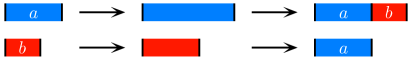
Figure 1. The geometric inflation rule for the Fibonacci chain, with natural tile lengths.

This way, one creates tilings $\mathcal{T}$ of the real line that give rise to a tiling space or hull

$$\mathbb{Y}\,=\,\overline{\{t+\mathcal{T}:t\in\mathbb{R}\}}\hskip 0.5pt,$$

where the closure is taken in the local topology. Here, two tilings are $\varepsilon$-close if they agree on the interval $\bigl{[}-\tfrac{1}{\varepsilon},\tfrac{1}{\varepsilon}\bigr{]}$, possibly after a small translation of one of them by at most $\varepsilon$. This gives the topological dynamical system $(\mathbb{Y},\mathbb{R})$, which is the continuous counterpart of the shift space $(\mathbb{X}_{0},\hskip 0.5pt\mathbb{Z})$ from above.

Any such tiling can be turned into a Delone set (a point set that is both uniformly discrete and relatively dense, see [8] for details) in many ways, perhaps the most common one emerging from taking the left endpoints of the intervals. They can be coloured if tiles of equal length have to be distinguished, as happens in all examples with degeneracies in the left PF eigenvector.

The tiling and the (possibly coloured) Delone set are locally equivalent in the sense that a strictly local rule exists to turn them into one another. They are thus mutually locally derivable (MLD). Such rules commute with the translation action and constitute an important subclass of topological conjugacies, which are homeomorphisms of the hull that commute with the translation action but need not stem from a local rule. This distinction will become important in the context of shape changes.

3. Embedding method

Returning to our guiding example, now in the form of a Fibonacci tiling (or point set), we look at the important set of translations that shift a tile (or a patch of tiles) to another occurrence within the same tiling, the so-called return vectors. Due to the inflation structure, we can do this for patches of arbitrary size in one step. Now, also taking all integer linear combinations of return vectors complete them into the return module, which is

$$\hskip 0.5pt\mathbb{Z}[\tau]\,=\,\{m+n\tau:m,n\in\hskip 0.5pt\mathbb{Z}\}\,=\,\hskip 0.5pt\mathbb{Z}\oplus\tau\hskip 0.5pt\mathbb{Z}$$

for our Fibonacci example. This is a $\hskip 0.5pt\mathbb{Z}$-module of rank $2$ that is a dense subset of $\mathbb{R}$. It can be seen as a projection of a lattice in $\mathbb{R}^{2}$ in many ways. A particularly natural one emerges from the Minkowski embedding as follows. Recall that algebraic conjugation in the quadratic field $\mathbb{Q}(\sqrt{5})$ is given by sending $\sqrt{5}$ to $-\sqrt{5}$. Denoting the corresponding mapping by $(.)^{\star}$, we can consider

$$\begin{split}\mathcal{L}\,&=\,\{(x,x^{\star}):x\in\hskip 0.5pt\mathbb{Z}[\tau]\}\\ &=\,\hskip 0.5pt\mathbb{Z}(1,1)\oplus\hskip 0.5pt\mathbb{Z}(\tau,1-\tau)\hskip 0.5pt,\end{split}$$

which is the lattice shown in Figure 2.

Figure 2. The Minkowski embedding of $\hskip 0.5pt\mathbb{Z}[\tau]$ as a planar lattice, where the projections are illustrated for the lattice point $(x,x^{\star})$ with $x=4+\tau$. The horizontal (vertical) axis represents the physical (internal) space.

Note that this lattice is neither a square nor a rectangular lattice, but by construction satisfies that its projection to the horizontal axis (the first coordinate) is $\hskip 0.5pt\mathbb{Z}[\tau]$. If one insists, a rescaling of the second coordinate can be used to turn $\mathcal{L}$ into a square lattice, compare [8, Rem. 3.4], but this brings no particular advantage. This just reflects the fact that the scale of internal space relative to physical space is arbitrary, and not a physically meaningful quantity.

The significant aspect of the return module and its embedding is the alternative description of the Fibonacci point set as a lattice projection set. If $\varLambda$ and $\varLambda^{\prime}$ are the Delone sets of the Fibonacci 2-cycle for $\rho_{1}$, one finds

$$\varLambda^{(\prime)}\,=\,\{x\in\hskip 0.5pt\mathbb{Z}[\tau]:x^{\star}\in W^{(\prime)}\}$$

where $W=(-1,\tau-1]$ and $W^{\prime}=[-1,\tau-1)$; see [8] for details. The difference between $\varLambda$ and $\varLambda^{\prime}$ consists in only two points, namely $-1$ (which belongs to $\varLambda^{\prime}$ but not to $\varLambda$) and $-\tau$ (which lies in $\varLambda$ but not in $\varLambda^{\prime}$). The union $\varLambda\cup\varLambda^{\prime}$ is coded by the closed interval $[-1,\tau-1]$ as window, and the existence of such two-sided asymptotic pairs is an essential feature for aperiodic, repetitive tilings. In fact, they are the reason why Bohr’s theory of almost periodic functions needs to be extended to cover these examples, as explained in some detail in [42].

There are several equivalent ways to view and interpret this projection approach. Here, a Euclidean cut-and-project scheme (CPS) is a triple $(\mathbb{R}^{n},\mathbb{R}^{m},\mathcal{L})$ with a lattice $\mathcal{L}\subset\mathbb{R}^{n+m}$ and two natural projections $\pi:\mathbb{R}^{n+m}\rightarrow\mathbb{R}^{n}$ and $\pi_{\text{int}}:\mathbb{R}^{n+m}\rightarrow\mathbb{R}^{m}$ satisfying that $\pi\bigl{|}_{\mathcal{L}}$ is injective and $\pi_{\text{int}}(\mathcal{L})$ is dense in $\mathbb{R}^{m}$. Since the projection $\pi$ restricted to the lattice $\mathcal{L}$ provides a bijection between the lattice $\mathcal{L}$ and $L=\pi(\mathcal{L})$, one defines the star map $\star:\mathbb{R}^{n}\rightarrow\mathbb{R}^{m}$ as

$$x\mapsto x^{\star}\mathrel{\mathop{:}}=\pi_{\text{int}}\bigl{(}\bigl{(}\pi\bigl{|}_{\mathcal{L}}\bigr{)}^{-1}(x)\bigr{)}.$$

This gives a rather natural connection between the physical space $\mathbb{R}^{n}$ and the internal space $\mathbb{R}^{m}$.

In our example, we have the following Euclidean CPS.

$$\begin{array}[]{ccccc@{}l}\mathbb{R}&\xleftarrow{\;\;\;\pi\;\;\;}&\mathbb{R}\times\mathbb{R}&\xrightarrow{\;\>\pi_{\text{int}}\;\>}&\mathbb{R}&\\ \cup&&\cup&&\cup&\raisebox{1.0pt}{\text{\scriptsize dense}}\\ \pi(\mathcal{L})&\xleftarrow{\;\hskip 0.5pt1-1\;\hskip 0.5pt}&\mathcal{L}&\xrightarrow{\qquad}&\pi_{\text{int}}(\mathcal{L})&\\ \|&&&&\|&\\ \,L=\hskip 0.5pt\mathbb{Z}[\tau]&\lx@intercol\hfil\xrightarrow{\qquad\qquad\;\,\star\;\,\qquad\qquad}\hfil\lx@intercol&\,{L}^{\star}=\hskip 0.5pt\mathbb{Z}[\tau]&\end{array}$$

Note that a CPS can be defined in the more general setting of $\sigma$-compact locally compact Abelian groups (and beyond) for both physical and internal space; see [8, 50, 60] for more.

One of the simplest examples that needs this more general type of CPS is the period doubling substitution $\varrho_{\mathrm{pd}}=(ab,aa)$. It is of constant length and has a coincidence (in the first position). It thus has pure point spectrum by Dekking’s criterion [27]. The corresponding CPS works with $\mathbb{R}$ as direct (or physical) space, as our guiding Fibonacci example. However, the internal space now is $\hskip 0.5pt\mathbb{Z}_{2}$, the 2-adic integers; see [8, Ex. 7.4] or [15] for more, and for an explicit diffraction formula.

A classic inflation rule over a ternary alphabet with a cubic inflation factor is given by the Tribonacci rule $\varrho_{\mathrm{Tri}}=(ab,ac,a)$, which also has a twisted version, namely $\varrho^{\prime}_{\mathrm{Tri}}=(ba,ac,a)$. Here, we need $\mathbb{R}$ as direct and $\mathbb{R}^{2}$ as internal space, where the windows are now Rauzy fractals, which are topologically regular sets (meaning that each is the closure of its interior); see [10, Fig. 1], and [53, 59, 60] for general background.

At this point, one might ask what happens if one extends the alphabet to an infinite one. Like in the case of Markov chains, things get more involved, but in the topological setting of compact alphabets, some systematic answers are possible; see [45] and references therein for an introduction. One important insight is that such a step produces many new phenomena, the perhaps most spectacular of which is the occurrence of inflation factors that need not be an algebraic integer, and can even be transcendental [32]. However, no analogue of the projection approach is known for this generalisation.

Figure 3. Diffraction of the visible lattice points. They have pure point (or Bragg) diffraction. The Bragg peaks are represented by disks whose area is the height (or intensity) of the peak, located at the centre of the disk; see [8, Thm. 10.5] for more.

An example of a totally different kind is provided by the square-free integers,

$$V_{2}\,=\,\Bigl{\{}x\in\hskip 0.5pt\mathbb{Z}:\mbox{\small\begin{tabular}[]{cc}$x$ is not divisible by the\\ square of any prime\end{tabular} }\Bigr{\}}.$$

It has holes of arbitrary size, but still pure point (or Bragg) diffraction [15]. Amazingly, it can also be described as a cut-and-project set, this time with a compact Abelian group $H$ as internal space. The corresponding window is a compact subset of $H$ that has no interior, but otherwise almost everything works as usual [55]. A planar counterpart is the set of visible lattice points of $\hskip 0.5pt\mathbb{Z}^{2}$, that is

$$V\,=\,\{(m,n)\in\hskip 0.5pt\mathbb{Z}^{2}:\gcd(m,n)=1\}\hskip 0.5pt.$$

It also admits a description via a suitable CPS, and leads to the diffraction image of Figure 3. For the details, see [8, Sec. 10.4.] as well as [15, 60] and references given there.

4. Variations and complications

Both $\rho_{1}$ and $\rho_{2}$ possess the substitution matrix $M$ from (2), and they are the only ones compatible with $M$. This is deceptively simple, as we can see from

$$M^{2}\,=\,\begin{pmatrix}2&1\\ 1&1\end{pmatrix}.$$

This matrix is compatible with precisely six substitution rules, namely

$${\rho_{1}}^{2}=(aba,ab), {\rho_{2}}^{2}=(aba,ba),$$

$$\rho_{1}\rho_{2}=(aab,ab), \rho_{2}\rho_{1}=(baa,ba),$$

which again define the Fibonacci system, together with the two previously mentioned rules

$$(aab,ba)\quad\mbox{and}\quad(baa,ab)\hskip 0.5pt.$$

They define an enantiomorphic pair of different systems (they both contain $bb$, unlike Fibonacci). Obviously, they are then no longer Sturmian, and hence more complex. Still, they admit self-similar tilings with the same intervals as used for the Fibonacci case, and thus with the same return module and the same CPS as in Eq. (3). Miraculously, they are also regular model sets, but with a much more complicated window. It is a natural question which condition would guarantee that the window is an interval. This has been studied extensively, and we refer readers to [19, 20, 22].

Considering $(aab,ba)$ one finds a particular window pair $W_{a},W_{b}$ of (genuine) Rauzy fractals with a fractal boundary, here of Hausdorff dimension

$$d_{\mathrm{H}}\,=\,\frac{\log(1+\sqrt{2})}{2\log(\tau)}\,\approx\,0,915{\hskip 0.5pt}785{\hskip 0.5pt}46\dots$$

Its partner system has windows $\widetilde{W}_{i}$ that are translates of the reflected windows, $-W_{i}$, as expected. A simple calculation reveals

$$\widetilde{W}_{a}\,=\,\tau-1-W_{a},\qquad\widetilde{W}_{b}\,=\,-1-W_{b}\hskip 0.5pt.$$

One can now imagine how this kind of complication might grow with the size of the matrix elements of the substitution matrix and even more so with the size of the alphabet. This is one of the reasons why the Pisot substitution conjecture for alphabets with more than two letters is still open [1]. Another reason is the unavoidability of Rauzy fractals even for the simplest inflations once the PF eigenvalue is an algebraic integer of degree three or higher; see [52, Prop. 2.35].

Let us briefly explore what else can happen as soon as we look for tilings of the plane. The direct product of two Fibonacci inflations can be encoded as shown in Figure 4, and nothing unexpected happens.

Figure 4. The Fibonacci direct product inflation rule in the Euclidean plane. Using the lower left corners as control points, one can extend the projection description of the Fibonacci chain to this case by doubling all dimensions and taking direct products of the 1D windows as the new windows here; see [3] for details.

But this is only the simplest of altogether $48$ possibilities to define a self-similar inflation with these tile shapes (and this inflation factor), but variations in the internal decomposition. As it turns out [3, 6], all of them are regular model sets, though some have windows of Rauzy fractal type, by which we mean that they have a fractal boundary. This adds another layer of complications one has to deal with, and the understanding of the possible windows with fractal boundary is far from complete. This kind of analysis opens the study of higher-dimensional inflation tilings. Clearly, there are also several variants of the famous Pisot conjecture [1], but a better understanding of the geometric constraints is required for future progress.

Further variations and generalisations of the Fibonacci tiling use another, very general approach to substitution tilings and their relatives, which is called fusion; see [31] for a detailed introduction. In the same paper, the scrambled Fibonacci tiling was introduced. This tiling still shares a lot of properties with the usual Fibonacci tiling, but it also serves as a counterintuitive example of pure-point diffractive structure which is not a Meyer set, as shown in [38]. Also, multi-scale variants have been considered, as well as concatenations of different rules (under the name $S$-adic substitutions); we refer to [45] and references therein for more.

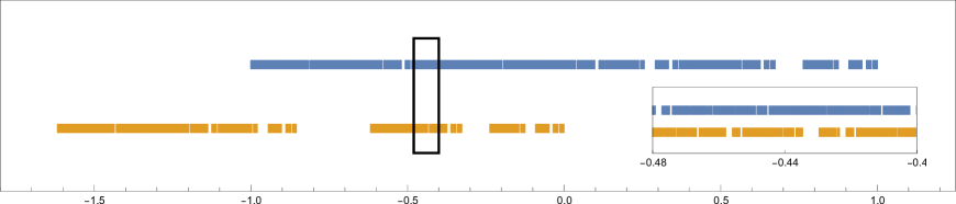
Figure 5. The two windows (blue/top for control points of type $a$ and yellow/bottom for type $b$) for the tiling given by the substitution $(aab,ba)$. The inlay shows a stretched view of the marked region. We emphasise that the sets $W_{a}$ and $W_{b}$ are measure-theoretically disjoint, see for example [60, Cor. 6.66], even though this is difficult to illustrate due to the high Hausdorff dimension of the boundaries.

Yet another direction was opened by random substitutions and inflations. The simplest example is based on the Fibonacci rules and can be given as

$$\varrho_{p}\,=\,(w_{p},a)\quad\mbox{with}\ w_{p}\,=\,\begin{cases}ab,&\mbox{with prob. }p,\\ ba,&\mbox{with prob. }1-p,\end{cases}$$

where the choice between $ab$ and $ba$ is randomly made at every step and position. This was introduced in [34], but largely neglected for a long time. A typical realisation of this rule, again with intervals of length $\tau$ and 1 as before, leads to a diffraction measure of mixed type, with pure point and absolutely continuous contributions; see [48] for further details and illustrations. Higher-dimensional examples are harder to find, due to geometric constraints, but have also been analysed (some already in [34]), and later systematically searched for in [33].

5. Equidistribution and ergodic aspects

Now, we ask what benefit we get from knowing that the Fibonacci point set $\varLambda$ is a model set, $\varLambda=\scalebox{1.3}{$\curlywedge$}(W)$ say with $W=[-1,\tau-1)$. The crucial observation is that $\varLambda^{\star}$ is uniformly distributed in $W$. To make sense of this statement, one has to turn the point set $\varLambda$ into a natural sequence, which is usually done by numbering its elements according to their distance from $0$, so we write $\varLambda=\{x_{n}\,:\,n\in\mathbb{N}\}$ with $|x_{n}|\leqslant|x_{n+1}|$ for all $n\in\mathbb{N}$. Then, the sequence $(x^{\star}_{n})_{n\in\mathbb{N}}$ is uniformly distributed in $W\!$, meaning that

$$\frac{\raisebox{-2.0pt}{$1$}}{\raisebox{0.5pt}{$N$}}\sum_{n=1}^{N}\mathbf{1}_{U}(x_{n})\,\xrightarrow{\hskip 0.5ptN\to\infty\hskip 0.5pt}\,\mathrm{vol}(U)$$

holds for every Borel subset $U\subseteq W\!$. The remaining freedom to arrange $\varLambda$ (when two elements have the same absolute value) is immaterial. The corresponding property holds for $\varLambda_{a}$ and $\varLambda_{b}$, where $\varLambda=\varLambda_{a}\,\dot{\cup}\,\varLambda_{b}$, relative to the windows $W_{a}$ and $W_{b}$; see [49] for a general account and further references, and [40] for a systematic treatment of equidistribution.

This property permits the determination of many frequencies coming from averages by calculating simple integrals. In other words, we have ergodicity. In almost all early papers, this property was tacitly assumed, though a proof came much later [57, 49], and these days is a consequence of some dynamical systems theory. The simplest application is the determination of the relative frequencies of points in $\varLambda$ of type $a$ and $b$, which gives $\tfrac{\mathrm{vol}(W_{a})}{\mathrm{vol}(W)}=\tau-1$ and $\tfrac{\mathrm{vol}(W_{B})}{\mathrm{vol}(W)}=2-\tau$, respectively. Clearly, we know this already from the PF right eigenvector of $M$, which seems equally easy. However, as soon as one proceeds to the calculation of general patch frequencies, the inflation method gets tedious, while the uniform distribution approach often remains straightforward and easily computable.

Let us explain this in some more detail for the Fibonacci tiling, formulated in terms of tiles (intervals) with their left endpoints as control points. They are all of the form

$$[m+n\tau,m+(n+1)\tau) \quad\mbox{for type}\ a,$$

$$[m+n\tau,m+1+n\tau) \quad\mbox{for type}\ b,$$

with $m,n\in\hskip 0.5pt\mathbb{Z}$, because $\varLambda\subset\hskip 0.5pt\mathbb{Z}[\tau]$ by construction (and every other Fibonacci tiling is a translate of one with this property). Now, each such interval has its own window in the internal space (as also shown in Figure 7), namely

(3) $$\begin{split}m+n(1-\tau)&+(1-\tau,\,2-\tau],\\ m+n(1-\tau)&+(2-\tau,\,1].\end{split}$$

So, if we are given a finite set of intervals (adjacent or not), we can decide on their joint legality in a Fibonacci point set within $\hskip 0.5pt\mathbb{Z}[\tau]$, and also determine the relative patch frequency as follows. Let $T_{1},\dots\,,T_{n}$ be these tiles, and $V_{1},\dots\,,V_{n}$ their windows according to (3). Then, we consider $V_{1}\cap\cdots\cap V_{n}$, and obtain

$$\mathrm{freq}\,(T_{1},\dots\,,T_{n})\,=\,\frac{\raisebox{-2.0pt}{$\mathrm{vol}(V_{1}\cap\cdots\cap V_{n})$}}{\raisebox{0.5pt}{$\mathrm{vol}(W)$}}\hskip 0.5pt,$$

which is $0$ whenever the patch is illegal (in the sense that it cannot occur in a single Fibonacci point set). With $V_{i}=(\alpha_{i},\beta_{i}]$, we simply get

$$\mathrm{vol}(V_{1}\cap\cdots\cap V_{n})\,=\,\min_{i}(\beta_{i})-\max_{j}(\alpha_{j})\hskip 0.5pt,$$

which is easy to implement.

This approach has analogues in higher dimensions, where the inflation method is quickly becoming impractical. In [47], based upon the dualisation method from [13, 39], the procedure is explained for the rhombic Penrose tiling and for the Ammann–Beenker tiling, where exact results are derived also for several large patches. The patch frequencies obtained this way have interesting applications in the theory of (discrete) Schrödinger operators on those tilings [26], in particular in connection with the support of localised eigenstates.

The frequency module of the Fibonacci tiling, which is $\hskip 0.5pt\mathbb{Z}[\tau]$, is the $\hskip 0.5pt\mathbb{Z}$-module of rank $2$ generated by the relative frequencies of words of length $2$ in the infinite Fibonacci word. It is not only helpful for patch frequencies, but also appears in the theory of one-dimensional aperiodic and ergodic Schrödinger operators. Indeed, consider the self-adjoint operator defined by

$$\bigl{(}H\psi\bigr{)}(n)\,=\,\psi(n+1)+\psi(n-1)+V(n)\,\psi(n)$$

on the Hilbert space $\ell^{2}(\hskip 0.5pt\mathbb{Z})$, with a potential function $V$ that takes two values according to the Fibonacci chain; see [25] for a detailed survey of the Fibonacci Hamiltonian. Then, its integrated density of states (IDS) is a devil’s staircase with plateaux where the IDS takes values from the frequency module. This is a topologically rigid structure that can be understood by Bellissard’s gap labeling theorem; see [17, 16, 11, 36] for details. Many open questions exist around this and related topological quantum numbers; see [37] for a survey.

6. Pair correlations

After this fairly general description of frequencies, let us look into the pair correlations in more detail. For this, let $\nu_{\alpha\beta}(z)$ be the relative frequency of a tile (or point) of type $\alpha$ and one of type $\beta$ occurring at distance $z\in\mathbb{R}$ within $\varLambda$. Clearly, this can only be non-zero for $z\in\varLambda-\varLambda\subset\hskip 0.5pt\mathbb{Z}[\tau]$, where

$$A-B=\{x-y\ :\ x\in A,\,y\in B\}$$

is the Minkowski difference of $A$ and $B$. In fact, $\nu_{\alpha\beta}(z)$ is positive if and only if $z\in\varLambda_{\alpha}-\varLambda_{\beta}$, and vanishes otherwise. This is a consequence of $\varLambda$ being a repetitive Delone set.

One can now use the method explained above. It can be simplified by observing that $z\in\varLambda_{\alpha}-\varLambda_{\beta}$ is equivalent to $z\in\hskip 0.5pt\mathbb{Z}[\tau]$ together with $z^{\star}\in W_{\alpha}-W_{\beta}$. Calculating the frequencies leads to

$$\nu_{\alpha\beta}(z)\,=\,g_{\alpha\beta}(z^{\star})$$

for $z\in\hskip 0.5pt\mathbb{Z}[\tau]$, with $g_{\alpha\beta}$ the simple continuous functions shown in Figure 6. Explicitly, the functions read

$$g_{aa}(y) =\max\bigl{(}\tfrac{1-|y|}{\tau},0\bigr{)},$$

$$g_{ba}(y) =\begin{cases}\frac{y}{\tau},&\mbox{if }0\leqslant y\leqslant\tau-1,\\ \frac{1}{\tau^{2}},&\mbox{if }\tau-1\leqslant y\leqslant 1,\\ 1-\frac{y}{\tau},&\mbox{if }1\leqslant y\leqslant\tau,\\ 0,&\mbox{otherwise,}\end{cases}$$

$$g_{bb}(y) =\max\bigl{(}\tfrac{1-\tau\hskip 0.5pt|y|}{\tau^{2}},0\bigr{)},$$

together with $g_{ab}(y)=g_{ba}(-y)$.

Figure 6. The continuous functions $g_{\alpha\beta}$ describing the pair correlations in internal space.

The total pair correlation (also known as the autocorrelation of $\varLambda$) is

(4) $$\nu(z)\,=\sum_{\alpha,\beta}\nu_{\alpha\beta}(z)\,=\,g(z^{\star}).$$

Here, $g(y)=\frac{1}{\tau}\bigl{(}\mathbf{1}_{-W}\ast\mathbf{1}_{W}\bigr{)}(y)$ is the covariogram of the total window, and similar representations hold for the $\nu_{\alpha\beta}$, namely

$$\nu_{\alpha\beta}(z)\,=\,\frac{\raisebox{-2.0pt}{$1$}}{\raisebox{0.5pt}{$\tau$}}\bigl{(}\mathbf{1}_{-W_{\alpha}}\ast\mathbf{1}_{W_{\beta}}\bigr{)}(z^{\star})\hskip 0.5pt,$$

which explains the result shown in Figure 6.

How is all this reflected in the inflation picture? As recently shown in [4, 5], the correlation coefficients satisfy the exact renormalisation relations

(5) $$\begin{split}\nu_{aa}(z)&=\tfrac{1}{\tau}\big{(}\nu_{aa}\big{(}\tfrac{z}{\tau}\big{)}+\nu_{ab}\big{(}\tfrac{z}{\tau}\big{)}\\ &\qquad\quad+\nu_{ba}\big{(}\tfrac{z}{\tau}\big{)}+\nu_{bb}\big{(}\tfrac{z}{\tau}\big{)}\big{)},\\ \nu_{ab}(z)&=\tfrac{1}{\tau}\big{(}\nu_{aa}\big{(}\tfrac{z}{\tau}-1\big{)}+\nu_{ba}\big{(}\tfrac{z}{\tau}-1\big{)}\big{)},\\ \nu_{ba}(z)&=\tfrac{1}{\tau}\big{(}\nu_{aa}\big{(}\tfrac{z}{\tau}+1\big{)}+\nu_{ab}\big{(}\tfrac{z}{\tau}+1\big{)}\big{)},\\ \nu_{bb}(z)&=\tfrac{1}{\tau}\nu_{aa}\big{(}\tfrac{z}{\tau}\big{)},\end{split}$$

with $z\in\varLambda-\varLambda$.

This is an infinite set of linear equations. A finite subset of them closes, namely the ones with $|z|\leqslant\tau$ on the left side. Subject to the constraints on the possible $z\in\varLambda-\varLambda$, this subset has a one-dimensional solution space, while all remaining coefficients are recursively determined from the ones of this subset. Specifying $\nu_{aa}(0)+\nu_{bb}(0)=1$ then gives the solution described above.

No similarly simple renormalisation seems to exist for $\nu(z)$. But one can use (4) together with (5) iteratively to derive the relation

$$\nu(z)\, =\,\frac{\raisebox{-2.0pt}{$1$}}{\raisebox{0.5pt}{$\tau^{2}$}}\,\nu\Bigl{(}\frac{\raisebox{-2.0pt}{$1$}}{\raisebox{0.5pt}{$\tau^{2}$}}\Bigr{)}\,+$$

$$\sum_{n\in\hskip 0.5pt\mathbb{Z}}\frac{\raisebox{-2.0pt}{$1$}}{\raisebox{0.5pt}{$\tau^{|n|+1}$}}\,\nu\biggl{(}\frac{\raisebox{-2.0pt}{$z+\mathrm{sgn}(n)\bigl{(}({-}\tau)^{|n|}-1\bigr{)}$}}{\raisebox{0.5pt}{$\tau^{|n|+1}$}}\biggr{)}$$

which can be interpreted in terms of the functions $g_{\alpha\beta}$ and rescaled/translated versions of them.

Now that we know the correlation coefficients for the self-similar Fibonacci tiling, it is an obvious question whether (and how) one can also get them for modified versions, in particular for the case that we use intervals of two arbitrary lengths. This is possible as long as the average interval length is $\tfrac{\sqrt{5}}{\tau}$, which is the one from our self-similar case. Other situations can be obtained from here by a simple global rescaling; see [46] for more.

7. Shape changes

To illustrate the effect of changing the relative tile lengths of the Fibonacci tiling, it is most convenient to view it as a section through a periodic array of atomic hypersurfaces (see Figure 7). This is equivalent to the cut-and-project construction, as explained in detail in [8, Sec. 7.5.1]. If we shear these atomic hypersurfaces parallel to the cut direction, maintaining the lattice sites at which they are attached, no vertices appear or disappear, nor change their type. Also, the periodicity of the array of hypersurfaces remains the same. The only effect is a change in the relative tile lengths. In Figure 7, we illustrate the change from original tile lengths (left) to all tile lengths equal (right). In the middle, both the sheared and unsheared hypersurfaces are displayed. As one can see, the deformed tiling is obtained by projecting the same lattice sites, which fall into the same window, along a new projection direction parallel to the sheared atomic hypersurfaces.

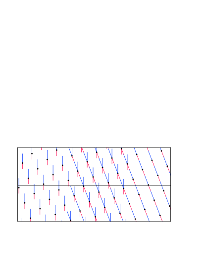
Figure 7. Original and sheared Fibonacci tiling, obtained as a section through a periodic array of atomic hypersurfaces.

The amount by which a vertex is moved depends non-locally on its environment. This length change is thus not locally derivable from the undeformed tiling, but it still induces a (non-local) topological conjugacy of the dynamical system, because it preserves the higher-dimensional lattice, and thus commutes with the translation action. In other words: the deformation does not mess up the aperiodic translational order. In fact, one can show [23, 24] that, as long as the overall scale is maintained, the Fibonacci tiling does not admit length changes which affect the dynamical system in a relevant way, which is a topological property of the Fibonacci hull; see [2, 56] for background on the topological methods applied here.

In the Hat and the Spectre tiling, the very same mechanism is at work. Both are obtained as shape changes from a cut-and-project tiling (with suitable control points), with copies of $\mathbb{R}^{2}$ as physical and internal spaces, and a four-dimensional lattice [7]. This explains their pure point diffraction property (which was numerically calculated in [63]), and their role as mathematical quasicrystals. The interesting feature in comparison to previous aperiodic monotiles is that they are quasiperiodic rather than limit-periodic (both in the sense of mean almost periodicity). It will be interesting to see which other tilings of this kind will be discovered, in particular in more than two dimensions.

8. Diffraction

Let us put all $\nu(z)$ in one object,

$$\gamma\,\mathrel{\mathop{:}}=\sum_{z\in\varLambda-\varLambda}\nu(z)\,\delta_{z}\hskip 0.5pt,$$

where $\delta_{z}$ is the Dirac measure (or distribution) at $z$. It is defined by $\delta_{z}(\phi)=\phi(z)$ for any function that is continuous at $z$. Here, $\gamma$ is a measure, and it is the natural autocorrelation measure of

$$\omega\,=\,\delta_{\!\varLambda}\,\mathrel{\mathop{:}}=\sum_{x\in\varLambda}\delta_{x}\hskip 0.5pt,$$

the Dirac comb of the point set $\varLambda$. It is usually defined as

$$\gamma\,=\lim_{n\to\infty}\frac{\raisebox{-2.0pt}{$1$}}{\raisebox{0.5pt}{$2n$}}\sum_{x,y\in\varLambda^{(n)}}\delta_{x-y}\hskip 0.5pt,$$

with $\varLambda^{(n)}=\varLambda\cap[-n,n]$. The existence of the limit is a consequence of the underlying ergodic properties of $\varLambda$. Here, $\gamma$ is a strongly almost periodic measure with Fourier transform

$$\widehat{\gamma}\,=\sum_{k\in L^{\circledast}}I(k)\,\delta_{k}$$

which is the diffraction measure of $\omega$. The supporting set is $L^{\circledast}=\hskip 0.5pt\mathbb{Z}[\tau]/\sqrt{5}$, also known as the dynamical or the Fourier–Bohr spectrum; see Section 9 for further details. It satisfies $L^{\circledast}=\pi(\mathcal{L}^{*})$, where $\mathcal{L}^{*}$ is the dual of the embedding lattice $\mathcal{L}$. The intensities at $k\in L^{\circledast}$ are given by $I(k)=|A(k)|^{2}$ with the amplitudes (or Fourier–Bohr coefficients)

$$A(k)\, =\lim_{n\to\infty}\frac{\raisebox{-2.0pt}{$1$}}{\raisebox{0.5pt}{$2n$}}\sum_{x\in\varLambda^{(n)}}\hskip 0.5pt\mathrm{e}^{-2\pi\hskip 0.5pt\mathrm{i}kx}$$

(6) $$=\,\begin{cases}\frac{\raisebox{-2.0pt}{$\mathrm{dens}(\varLambda)$}}{\raisebox{0.5pt}{$\mathrm{vol}(W)$}}\;\widehat{\mathbf{1}_{W}}(-k^{\star}),&\mbox{if}\ k\in L^{\circledast},\\ 0,\ &\mbox{otherwise},\end{cases}$$

where the limit always exists; see [12] for an elementary proof of this formula.

The importance of the FB coefficients can hardly be overstated. They are also instrumental in the recent classification of pure point diffraction via almost periodicity [42, 43], and they play an important role in the dynamical systems approach to aperiodic order, as we shall see in Section 9.

More generally, one is interested in weighted Fibonacci combs, such as

$$\omega\,=\,h_{a}\hskip 0.5pt\delta_{\!\varLambda_{a}}+h_{b}\hskip 0.5pt\delta_{\!\varLambda_{b}}\hskip 0.5pt,$$

which gives scattering strength $h_{\alpha}$ to points of type $\alpha$. Now, the autocorrelation becomes

$$\gamma\, \,=|h_{a}|^{2}\,\gamma_{aa}+h_{a}\,\overline{h_{b}}\,\gamma_{ab}$$

$$\qquad+\overline{h_{a}}\,h_{b}\,\gamma_{ba}+|h_{b}|^{2}\,\gamma_{bb}$$

with diffraction

$$\widehat{\gamma}\,=\sum_{k\in L^{\circledast}}\bigl{|}h_{a}A_{a}(k)+h_{b}A_{b}(k)\bigr{|}^{2}\,\delta_{k}\hskip 0.5pt,$$

where $A_{\alpha}(k)$ is the FB coefficient of $\delta_{\!\varLambda_{\alpha}}$ at $k$. The formula reflects the phase consistency property as proved in [5, 42]. More general weighting schemes can be considered, as outlined in [66].

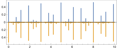
Figure 8. The diffraction image for the Fibonacci tiling (yellow, bottom) and for the reshuffled Fibonacci (blue, top) for $0\leqslant k\leqslant 10$. The intensity of every Bragg peak (the absolute square of the Fourier–Bohr coefficient) is given by the height of the bar. The intensity of the central peak at $0$ is $(\tau+1)/5\approx 0.5236$.

In Figure 8, we show the diffraction of the Fibonacci chain in comparison to the one from the reshuffled version. The latter has the much more complicated windows from Figure 5 with their fractal boundaries. In fact, calculating the FB coefficients for them requires a method from [10] to calculate $\widehat{\mathbf{1}_{W}}$, which is based on the Fourier matrix cocycle. Note that a numerical approach via the Fourier transform of large finite patches converges in principle, but rather slowly.

This is actually a typical situation, which is not restricted to windows in one dimension. It also arises in the case of the (twisted) Tribonacci inflation $\varrho^{(\prime)}_{\mathrm{Tri}}$ mentioned earlier, where the windows are two-dimensional Rauzy fractals. In the standard case, the windows are simply connected, and the numerical approach still works reasonably well, while it fails rather badly for the twisted case, where the windows are ‘spongy’. This was studied in more details for the plastic number inflation in [9], which has windows of a similar type. Also, the difficulty of a reliable (numerical) calculation increases with the Hausdorff dimension of the boundary.

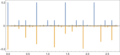
Figure 9. Diffraction of the symbolic Fibonacci chain with equal tile lengths of $\sqrt{5}/\tau$ and weights $h_{a}=1$, $h_{b}=0$ (blue, top) and in comparison to its geometric realization with natural tile lengths $\tau$ and $1$ (yellow, bottom). The intensity of the central peak at $0$ is $1/5$ and the peaks are shown for wave numbers in $[0,2\sqrt{5}/\tau)$, which corresponds to two fundamental cells of the average lattice underneath the symbolic case.

Let us also mention that the embedding formalism also permits to calculate the diffraction of the Fibonacci chain under the shape changes illustrated in Figure 7. This results in deformed model sets, compare [8, Ex. 9.9] for a related example and [18] for a general discussion, which still leads to a closed formula for the diffraction. Figure 9 illustrates the result for the extreme case that the interval lengths become equal. The aperiodicity is still present (via two differend weights for the point types) and clearly visible from the peaks, despite the fact that the (coloured) points now live on a lattice. In this case, in line with [8, Thm. 10.3], the diffraction measure is periodic. The analogous situation occurs for the Hat tiling [7], then with a hexagonal lattice.

In two dimensions, among the most prominent examples are the rhombic Penrose, the Ammann–Beenker (AB), and the square-triangle tiling due to Schlottmann [8, Sec. 6.3.1], with $10$-, $8$- and $12$-fold symmetry, respectively. The CPS is simplest for the AB tiling, producing for instance the symmetric patch and the diffraction image of Figure 10. This is based on the lattice $\hskip 0.5pt\mathbb{Z}^{4}$ in $\mathbb{R}^{4}$; see [8, Ex. 7.8] for details. The vertices of the rhombic Penrose tiling fall into four distinct translation classes, as analysed in detail in [13], thus completing the pioneering work by de Bruijn [29]. The square-triangle tiling is the most difficult of these three, because it has a window with twelvefold symmetry but fractal boundary. This is unavoidable for square-triangle tilings, and one inflation tiling of this kind, due to Schlottmann, is described in detail in [8, Sec. 6.3.1 and Fig. 7.10].

Figure 10. The left panel shows a finite, eightfold symmetric patch of the Ammann–Beenker tiling. The vertex points can be obtained as a model set via the hypercubic lattice and a regular octagon as window in internal space. The right panel displays the diffraction of the (infinite) Ammann–Beenker model set. Bragg peaks are again represented as disks, as in Figure 3

9. Dynamical systems approach

The dynamical systems mentioned earlier have always been important objects of mathematical research, but their importance was hardly recognised in physics. This changed in the context of aperiodic order, where they bring important insight. Let us explain this with the Fibonacci tiling dynamical system $(\mathbb{Y},\mathbb{R})$ from Section 2. Since $\mathbb{Y}$ is compact, there exists (by general arguments) at least one probability measure that is invariant under the translation action. In fact, in this example, there is precisely one such measure, $\mu_{{}_{\mathrm{F}}}$, and this turns the topological dynamical system $(\mathbb{Y},\mathbb{R})$ into a measure-theoretical one, denoted by $(\mathbb{Y},\mathbb{R},\mu_{{}_{\mathrm{F}}})$.

The measure $\mu_{{}_{\mathrm{F}}}$ is ergodic (every invariant subset of $\mathbb{Y}$ has either measure 0 or 1), and all averages along Fibonacci chains can be written as integrals over $\mathbb{Y}$ with respect to $\mu_{{}_{\mathrm{F}}}$. Another connection concerns the spectral theory of the Fibonacci chain. Given $\mathbb{Y}$ and $\mu_{{}_{\mathrm{F}}}$, one can define the Hilbert space $L^{2}(\mathbb{Y},\mu_{{}_{\mathrm{F}}})$ of square-integrable functions $f:\mathbb{Y}\rightarrow\mathbb{C}$, where the inner product is given by

$$\langle g\hskip 0.5pt\hskip 0.5pt|\hskip 0.5ptf\rangle\,\mathrel{\mathop{:}}=\int_{\mathbb{Y}}\,\overline{g(Y)}f(Y)\,\mathrm{d}\hskip 0.5pt\mu_{{}_{\mathrm{F}}}(Y)\hskip 0.5pt.$$

The crucial observation, due to Koopman, now is that the translation action on the tiling space induces a family of unitary operators $T_{t}$ on $L^{2}(\mathbb{Y},\mu_{{}_{\mathrm{F}}})$ via $(T_{t}f)(Y)\mathrel{\mathop{:}}=f(Y\!{-}\hskip 0.5ptt)$, where $Y\in\mathbb{Y}$ is a tiling and $Y\!{-}\hskip 0.5ptt$ its translate. Indeed, for arbitrary $f,g\in L^{2}(\mathbb{Y},\mu_{{}_{\mathrm{F}}})$, one gets

$$\begin{split}\langle T_{t}g\hskip 0.5pt\hskip 0.5pt|\hskip 0.5ptT_{t}f\rangle\,&=\int_{\mathbb{Y}}\,\overline{g(Y\!{-}\hskip 0.5ptt)}f(Y\!{-}\hskip 0.5ptt)\,\mathrm{d}\hskip 0.5pt\mu_{{}_{\mathrm{F}}}(Y)\\[2.84526pt] &=\int_{\mathbb{Y}}\,\overline{g(Y)}f(Y)\,\mathrm{d}\hskip 0.5pt\mu_{{}_{\mathrm{F}}}(Y)\,=\,\langle g\hskip 0.5pt\hskip 0.5pt|\hskip 0.5ptf\rangle,\end{split}$$

where the second step follows by a change of variable transform and the translation invariance of $\mu_{{}_{\mathrm{F}}}$.

Since the $T_{t}$ commute with one another for all $t\in\mathbb{R}$, the operators possess simultaneous eigenfunctions (if any), and the remarkable property here is that there is a (countable) set of eigenfunctions which span $L^{2}(\mathbb{Y},\mu_{{}_{\mathrm{F}}})$. One then says that $(\mathbb{Y},\mathbb{R},\mu_{{}_{\mathrm{F}}})$ has pure point dynamical spectrum. The theory of such systems was developed by Halmos and von Neumann [35], and is a cornerstone of dynamical systems theory. Here, the connection can be made more concrete, which gives a link to diffraction theory; see [65, 54, 14] and references therein.

Let us select a Fibonacci point set $\varLambda$, the point set of a tiling $Y\in\mathbb{Y}$, and consider the corresponding Fourier–Bohr coefficient $A_{\!\varLambda}(k)=A(k)$ as defined in Eq. (6) for arbitrary $k\in\mathbb{R}$, often called the wave number. In physics, this is the (complex) amplitude of the structure. The strong ergodicity of $\mu_{{}_{\mathrm{F}}}$ implies that the limit always exists, and one obtains the formula given in (6), with $W=[-1,\tau-1)$ if $\varLambda$ is our Fibonacci point set from above and ^⋆ is the star map. In diffraction, as explained earlier, we get the intensity of the Bragg peak at $k$ as $I(k)=|A_{\!\varLambda}(k)|^{2}$.

The connection to dynamics now comes from the observation how $A_{\!\varLambda}(k)$ behaves under translations of $\varLambda$, where we get

$$A_{t+\varLambda}(k)\,=\,\hskip 0.5pt\mathrm{e}^{-2\pi\hskip 0.5pt\mathrm{i}kt}A_{\!\varLambda}(k)\hskip 0.5pt,$$

for all $k\in\mathbb{R}$. When $A_{\!\varLambda}(k)\neq 0$, which is true unless we hit an exceptional extinction point, this can be considered as an eigenfunction equation with eigenvalue $\hskip 0.5pt\mathrm{e}^{-2\pi\hskip 0.5pt\mathrm{i}kt}$. To avoid the appearance of extinctions, one can consider a Dirac comb with different weights for points of type $a$ and $b$, and define the FB coefficients accordingly. Then, generically, there are no extinctions, and one obtains a complete set of eigenfunctions. In our guiding example, they turn out to be continuous on $\mathbb{Y}$, and are thus called topological eigenvalues; see [37] for interesting connections with topological invariants.

Since $\mathbb{R}$ is a continuous group, it is advantageous to use the wave numbers $k$ to label the eigenvalues. Thus, $L^{\circledast}=\hskip 0.5pt\mathbb{Z}[\tau]/\sqrt{5}$ is called the dynamical spectrum of $(\mathbb{Y},\mathbb{R},\mu_{{}_{\mathrm{F}}})$ in additive notation.

A fundamental insight (based on Dworkin’s argument [30, 28]) now is that a Delone dynamical system (such as our Fibonacci model set) has pure point dynamical spectrum if and only if the diffraction measure of a typical element of the tiling hull has pure point (or Bragg) diffraction [14, 41, 44]. In good cases (such as our guiding example), every element is typical, in others (such as the visible lattice points), one has to make the correct choice. This connection is also instrumental in the recent analysis of pure point diffraction via averaged versions of almost periodicity; see [42] and references therein for more.

References

- [1] S. Akiyama, M. Barge, V. Berthé, J.-Y. Lee and A. Siegel, On the Pisot substitution conjecture, in Mathematics of Aperiodic Order, eds. J. Kellendonk, D. Lenz and J. Savinien, Birkhäuser, Basel (2015), pp. 33–72.
- [2] J.E. Anderson and I.F. Putnam, Topological invariants for substitution tilings and their associated -algebras, Ergod. Th. Dynam. Syst. 18 (1998), 509–537.
- [3] M. Baake, N.P. Frank and U. Grimm, Three variations on a theme by Fibonacci, Stoch. Dyn. 21 (2021), 2140001:1–23; arXiv:1910.00988.
-
[4]
M. Baake and F. Gähler,
Pair correlations of aperiodic inflation rules via renormalisation:
Some interesting examples,
Topol. Appl. 205 (2016), 4–27;
arXiv:1511.00885. - [5] M. Baake, F. Gähler and N. Mañibo, Renormalisation of pair correlation measures for primitive inflation rules and absence of absolutely continuous diffraction, Commun. Math. Phys. 370 (2019), 591–635; arXiv:1805.09650.
- [6] M. Baake, F. Gähler and J. Mazáč, Fibonacci direct product tiling variations J. Math. Phys. 63 (2022), 082702:1–13; arXiv:2203.07743 .
-
[7]
M. Baake, F. Gähler and L. Sadun,
Dynamics and topology of the Hat family of tilings,
preprint;
arXiv:2305.05639. - [8] M. Baake and U. Grimm, Aperiodic Order. Vol. 1: A Mathematical Invitation, Cambridge University Press, Cambridge (2013).
- [9] M. Baake and U. Grimm, Diffraction of a model set with complex windows, J. Phys.: Conf. Ser. 1458 (2020), 012006:1–6; arXiv:1904.08285.
- [10] M. Baake and U. Grimm, Fourier transform of Rauzy fractals and point spectrum of 1D Pisot inflation tilings, Docum. Math. 25 (2020), 2303–2337; arXiv:1907.11012.
- [11] M. Baake, U. Grimm and D. Joseph, Trace maps, invariants, and some of their applications, Int. J. Mod. Phys. B 7 (1993), 1527–1550; arXiv:math-ph/9904025.
- [12] M. Baake and A. Haynes, Convergence of Fourier–Bohr coefficients for regular Euclidean model sets, preprint; arXiv:2308.07105.
- [13] M. Baake, P. Kramer, M. Schlottmann and D. Zeidler, Planar patterns with fivefold symmetry as sections of periodic structures in 4-space, Int. J. Mod. Phys. B 4 (1990), 2217–2268.
- [14] M. Baake and D. Lenz, Dynamical systems on translation bounded measures: Pure point dynamical and diffraction spectra, Ergod. Th. Dynam. Syst. 24 (2004), 1867–1893; arXiv:math.DS/0302061.
- [15] M. Baake, R.V. Moody and P.A.B. Pleasants, Diffraction or visible lattice points and th power free integers, Discr. Math. 221 (2000), 3–42; arXiv:math.MG/9906132.
- [16] J.V. Bellissard, A. Bovier and J. M. Ghez, Gap labelling theorems for one-dimensional discrete Schrödinger operators, Rev. Math. Phys. 4 (1992), 1–37.
-
[17]
J.V. Bellissard, B. Iochum, E. Scoppola and D. Testard,
Spectral properties of one-dimensional quasi-crystals,
Commun. Math. Phys. 125 (1989), 527–543. - [18] G. Bernuau and M. Dunau, Fourier analysis of deformed model sets, in Directions in Mathematical Quasicrystals, eds. M. Baake and R. V. Moody, Fields Institute Monographs, vol. 13, Amer. Math. Society, Providence, RI (2000), pp. 43–60.
- [19] V. Berthé, H. Ei, S. Ito and H. Rao, On substitution invariant Sturmian words: An application of Rauzy fractals, RAIRO – Theor. Inform. Appl. 41 (2007), 329–349.
- [20] V. Berthé, D. Frettlöh and V. Sirvent, Selfdual substitutions in dimension one, Eur. J. Comb. 33 (2012), 981–1000; arXiv:1108.5053.
- [21] H. Bohr, Almost Periodic Functions, reprint, Chelsea, New York (1947).
- [22] V. Canterini, Connectedness of geometric representation of substitutions of Pisot type, Bull. Belg. Math. Soc. Simon Stevin 10 (2003), 77–89.
-
[23]
A. Clark and L. Sadun,
When size matters,
Ergod. Th. Dynam. Syst. 23 (2003), 1043–1057;
arXiv:math.DS/0201152. - [24] A. Clark and L. Sadun, When shape matters, Ergod. Th. Dynam. Syst. 26 (2006), 69–86; arXiv:math.DS/0306214.
- [25] D. Damanik, A. Gorodetski and W. Yessen, The Fibonacci Hamiltonian, Inv. Math. 206 (2016), 629–692; arXiv:1403.7823.
- [26] D. Damanik, M. Embree, J. Fillman and M. Mei, Discontinuities of the integrated density of states for Laplacians associated with Penrose and Ammann–Beenker tilings, Exp. Math. (2023), 1–23; arXiv:2209.01443.
- [27] F.M. Dekking, The spectrum of dynamical systems arising from substitutions of constant length, Z. Wahrscheinlichkeitsth. Verw. Geb. 41 (1978), 221–239.
- [28] X. Deng and R.V. Moody, Dworkin’s argument revisited: point processes, dynamics, diffraction, and correlations J. Geom. Phys. 58 (2008), 506–541.
- [29] N.G. de Bruijn, Algebraic theory of Penrose’s non-periodic tilings of the plane, I & II, Kon. Nederl. Akad. Wetensch. Proc. Ser. A 84 (1981), 39–52 and 53–66.
- [30] S.Dworkin, Spectral theory and X-ray diffraction, J. Math. Phys. 34 (1993), 2965–2967.
- [31] N.P. Frank and L. Sadun, Fusion: a general framework for hierarchical tilings of , Geom. Dedicata 171 (2014), 149–186; arXiv:1101.4930.
-
[32]
D. Frettlöh, A. Garber, N. Mañibo,
Substitution tilings with transcendental inflation factor,
Discr. Anal., to appear;
arXiv:2208.01327. - [33] F. Gähler, E.E. Kwan, G.R. Maloney, A computer search for planar substitution tilings with -fold rotational symmetry, Discr. Comput. Geom. 53 (2015), 445–465; arXiv:1404.5193.
- [34] C. Godrèche and J.M. Luck, Quasiperiodicity and randomness in tilings of the plane, J. Stat. Phys. 55 (1989), 1–28.
- [35] P.R. Halmos and J. von Neumann, Operator methods in classical mechanics. II. Ann. Math. 43 (1944), 332-350.
- [36] J. Kellendonk, Noncommutative geometry of tilings and gap labelling, Rev. Math. Phys. 7 (1995), 1133–1180; arXiv:cond-mat/9403065.
- [37] J. Kellendonk, Topological quantum numbers in quasicrystals, preprint, this issue.
- [38] J. Kellendonk and L. Sadun, Meyer sets, topological eigenvalues, and Cantor fiber bundles, J. London Math. Soc. 89 (2014), 114–130; arXiv:1211.2250.
- [39] P. Kramer and M. Schlottmann, Dualisation of Voronoi domains and klotz construction: a general method for the generation of proper space fillings, J. Phys. A: Math. Gen. 22 (1989), L1097–L1102.
- [40] L. Kuipers and H. Niederreiter, Uniform Distribution of Sequences, reprint, Dover, New York (2006).
- [41] J.-Y. Lee, R.V. Moody and B. Solomyak, Pure point dynamical and diffraction spectra, Ann. H. Poincaré 2 (2002), 1003–1018; arXiv:0910.4809.
- [42] D. Lenz, T. Spindeler and N. Strungaru, Pure point spectrum for dynamical systems and mean almost periodicity, preprint; arXiv:2006.10825.
- [43] D. Lenz, T. Spindeler and N. Strungaru, Almost periodicity and pure point diffraction, preprint, this issue.
-
[44]
D. Lenz and N. Strungaru,
Pure point spectrum for measure dynamical systems on locally
compact Abelian groups,
J. Math. Pures Appl. 92 (2009), 323–341;
arXiv:0704.2498. - [45] N. Mañibo, Substitutions and generalisations, preprint, this issue.
- [46] J. Mazáč, PhD thesis, in preparation.
- [47] J. Mazáč, Patch frequencies in Penrose rhombic tilings, Acta Cryst. A 79 (2023), 399–411; arXiv:2212.09406.
- [48] M. Moll, On a Family of Random Noble Means Substitutions, PhD thesis (Bielefeld University, 2013); available electronically at urn:nbn:de:hbz:361-26378078.
- [49] R.V. Moody, Uniform distribution in model sets, Can. Math. Bull. 45 (2002), 123–130.
- [50] R.V. Moody, Model sets: a survey, in From Quasicrystals to More Complex Systems, eds. F. Axel, F. Dénoyer and J.P. Gazeau, Springer, Berlin (2000), pp. 145–166; arXiv:math.MG/0002020.
- [51] R.V. Moody and J.-Y. Lee, Taylor–Socolar hexagonal tilings as model sets, Symmetry 5 (2013), 1–46; arXiv:1207.6237.
- [52] P.A.B. Pleasants, Designer quasicrystals: cut-and-project sets with pre-assigned properties, in Directions in Mathematical Quasicrystals, eds. M. Baake and R. V. Moody, Fields Institute Monographs, vol. 13, Amer. Math. Society, Providence, RI (2000), pp. 95–141.
- [53] N. Pytheas Fogg, Substitutions in Dynamics, Arithmetics and Combinatorics, eds. V. Berthé, S. Ferenczi, C. Mauduit and A. Siegel, LNM 1794, Springer, Berlin (2002).
- [54] M. Queffélec, Substitution Dynamical Systems: Spectral Analysis, 2nd ed., LNM 1294, Springer, Berlin (2010).
- [55] C. Richard and N. Strungaru, Pure point diffraction and Poisson summation, Ann. Henri Poincaré 18 (2017), 3903–3931; arXiv:1512.00912
- [56] L. Sadun, Topology of Tiling Spaces, Amer. Math. Society, Providence, RI (2008).
- [57] M. Schlottmann, Cut-and-project sets in locally compact Abelian groups, in Quasicrystals and Discrete Geometry, ed. J. Patera, Fields Institute Monographs, vol. 10, Amer. Math. Society, Providence, RI (1998), pp. 247–264.
- [58] D. Shechtman, I. Blech, D. Gratias and J.W. Cahn, Metallic phase with long-range orientational order and no translational symmetry, Phys. Rev. Lett. 53 (1984), 1951–1953.
- [59] A. Siegel, J.M. Thuswaldner, Topological properties of Rauzy fractals, Les Mémoires de la SMF 118 (2009).
- [60] B. Sing, Pisot Substitutions and Beyond, PhD thesis (Bielefeld University, 2007); available electronically at urn:nbn:de:hbz:361-11555.
-
[61]
D. Smith, J.S. Myers, C.S. Kaplan and C. Goodman-Strauss,
An aperiodic monotile, preprint;
arXiv:2303.10798. -
[62]
D. Smith, J.S. Myers, C.S. Kaplan and C. Goodman-Strauss,
A chiral aperiodic monotile, preprint;
arXiv:2305.17743. - [63] J.E.S. Socolar, Quasicrystalline structure of the Smith monotile tilings, preprint; arXiv:2305.01174.
-
[64]
J.E.S. Socolar and J.M. Taylor,
An aperiodic hexagonal tile,
J. Comb. Th. A 118 (2011), 2207–2231;
arXiv:1003.4279. - [65] B. Solomyak, Dynamics of self-similar tilings, Ergod. Th. Dynam. Syst. 17 (1997), 695–738 and Ergod. Th. Dynam. Syst. 19 (1999), 1685 (erratum).
-
[66]
N. Strungaru,
Almost periodic pure point measures, in
Aperiodic Order. Vol. 2: Crystallography and
Almost Periodicity, eds. M. Baake and U. Grimm,
Cambridge University Press, Cambridge (2017), pp. 271–342;
arXiv:1501.00945.