Splitting the Conditional Gradient Algorithm

Abstract

We propose a novel generalization of the conditional gradient (CG / Frank-Wolfe) algorithm for minimizing a smooth function $f$ under an intersection of compact convex sets, using a first-order oracle for $\nabla f$ and linear minimization oracles (LMOs) for the individual sets. Although this computational framework presents many advantages, there are only a small number of algorithms which require one LMO evaluation per set per iteration; furthermore, these algorithms require $f$ to be convex. Our algorithm appears to be the first in this class which is proven to also converge in the nonconvex setting. Our approach combines a penalty method and a product-space relaxation. We show that one conditional gradient step is a sufficient subroutine for our penalty method to converge, and we provide several analytical results on the product-space relaxation’s properties and connections to other problems in optimization. We prove that our average Frank-Wolfe gap converges at a rate of $\mathcal{O}(\ln t/\sqrt{t})$, – only a log factor worse than the vanilla CG algorithm with one set.

Keywords. Conditional gradient, splitting, nonconvex, Frank-Wolfe, projection free

MSC Classification. 46N10, 65K10, 90C25, 90C26, 90C30

1 Introduction

Given a smooth function $f$ which maps from a real Hilbert space $\mathcal{H}$ to $\mathbb{R}$ and a finite collection of $m$ nonempty compact convex subsets $(C_{i})_{i\in I}$ of $\mathcal{H}$, we seek to solve the following:

$$\text{minimize}\;\;f(x)\quad\text{subject to}\quad x\in\bigcap_{i\in I}C_{i},$$ (1)

which has many applications in imaging, signal processing, and data science [1, 2, 3]. Classical projection-based algorithms can be used to solve (1) if given access to the operator $\text{\rm Proj}\,_{\bigcap_{i\in I}C_{i}}$. However, in practice, computing a projection onto $\bigcap_{i\in I}C_{i}$ is either impossible or numerically costly, and utilizing the individual projection operators $(\text{\rm Proj}\,_{C_{i}})_{i\in I}$ is more tractable. This issue has given rise to the advent of splitting algorithms, which seek to solve (1) by utilizing operators associated with the individual sets – not their intersection. Projection-based splitting algorithms – which use the collection of operators $(\text{\rm Proj}\,_{C_{i}})_{i\in I}$ instead of $\text{\rm Proj}\,_{\bigcap_{i\in I}C_{i}}$ – have made previously-intractable problems of the form (1) solvable with simpler tools on a larger scale [1, 3, 4].

While splitting methods have successfully been applied to projection-based algorithms, relatively little has been done for the splitting of conditional gradient (CG / Frank-Wolfe) algorithms. Standard CG algorithms minimize a smooth function $f\colon\mathbb{R}^{n}\to\mathbb{R}$ over one closed convex constraint set $C\subset\mathbb{R}^{n}$. While the iterates of this algorithm do not converge in general [5], at iteration $t\in\mathbb{N}$, the average Frank-Wolfe gap (which is closely related to showing Clarke stationarity [6]) converges at a rate of $\mathcal{O}(1/\sqrt{t})$, and the primal gap converges at a rate of $\mathcal{O}(1/t)$ when $f$ is convex [7]. A key ingredient of these algorithms is the linear minimization oracle, $\operatorname{LMO}_{C}$, which computes for a linear objective $c\in\mathbb{R}^{n}$ a point in ${\text{\rm Argmin}}\,_{x\in C}\langle c\,,\,x\rangle$. Similarly to traditional projection-based methods, computing $\operatorname{LMO}_{\bigcap_{i\in I}C_{i}}$ is often prohibitively costly, so an algorithm which relies on the individual operators $(\operatorname{LMO}_{C_{i}})_{i\in I}$ would be more tractable.

In principle, if two sets $C_{1}$ and $C_{2}$ are polytopes, one could compute $\operatorname{LMO}_{C_{1}\cap C_{2}}$ by solving a linear program which incorporates the LP formulations of both $C_{1}$ and $C_{2}$. However, since the number of inequalities in an LP formulation can scale exponentially with dimension [8, 6], LPs are usually only used to implement a polyhedral LMO if there are no alternatives. In reality, many polyhedra used in applications, e.g., the Birkhoff polytope and the $\ell_{1}$ ball, have highly specialized algorithms for computing their LMO which are faster than using a linear program [9]. Hence, splitting algorithms which rely on evaluating the specialized algorithms for $(\operatorname{LMO}_{C_{i}})_{i\in I}$ gain the favorable scalability of existing LMO implementations.

Conditional gradient methods have seen a resurgence in popularity since, particularly for high-dimensional settings, LMOs can be more computationally efficient than projections. For instance, a common constraint in matrix completion problems is the spectrahedron

$$S=\{x\in\mathbb{S}^{n}_{+}\,|\,\text{Trace}(x)=1\},$$ (2)

where $\mathbb{S}_{+}^{n}$ is the set of positive semidefinite $n\times n$ matrices. Evaluating $\text{\rm Proj}\,_{S}$ requires a full eigendecomposition, while computing $\operatorname{LMO}_{S}$ only requires determining a dominant eigenpair [10]. Clearly, there are high-dimensional settings where evaluating $\operatorname{LMO}_{S}$ is possible while $\text{\rm Proj}\,_{S}$ is too costly [9]. Thus, we are particularly motivated by high-dimensional problems in data science (e.g., cluster analysis, graph refinement, and matrix decomposition) with these LMO-advantaged constraints, e.g., the nuclear norm ball, the Birkhoff polytope of doubly stochastic matrices, and the $\ell_{1}$ ball [6, 10, 11, 12, 13, 14, 15].

Inexact proximal splitting methods are a natural choice for solving (1) in our computational setting, since LMO-based subroutines can approximate a projection. In the convex case, this approach appears in [16, 17, 18, 19]. However, there is often no bound on the number of LMO calls required to meet the relative error tolerance required of the subroutine, e.g., in [19]. Methods which require increasingly-accurate approximations can drive the number of LMO calls in each subroutine to infinity [18], and even if a bound on the number of LMO calls exists, it often depends on the conditioning of the projection subproblem.

We are interested in algorithms with low iteration complexity, since they are more tractable on large-scale problems. It appears that, for this computational setting, the lowest iteration complexity currently requires one LMO per set per iteration [20, 2, 12, 21, 22, 23]. To the best of our knowledge, all algorithms in this class are restricted to the convex setting. The case when $f=0$ is addressed by [20], the case when $(C_{i})_{i\in I}$ have additional structure is addressed in [21], and a matrix recovery problem is addressed in [22]. The approaches in [2, 12, 23] essentially show that one CG step is a sufficient subroutine for an inexact augmented Lagrangian (AL) approach. These methods prove convergence of different optimality criteria at various rates, e.g., arbitrarily close to $\mathcal{O}(t^{-1/3})$ [2], $\mathcal{O}(1/\sqrt{t})$ [23, 21], and (under restrictions on $m$ or $(C_{i})_{i\in I}$) $\mathcal{O}(1/t)$ [12, 22, 20]. All of these methods, similarly to many projection-based splitting algorithms, achieve approximate feasibility in the sense that a point in the intersection $\bigcap_{i\in I}C_{i}$ is only found asymptotically.

Our contributions are as follows. We propose a new algorithm in this class for solving (1) which requires one LMO per set per iteration. Our algorithm generalizes the vanilla CG algorithm in the sense that, when $m=1$, both algorithms are identical. It appears that our algorithm is the first in this class possessing convergence guarantees for solving (1) in the setting when $f$ is nonconvex. As is standard in the CG literature, we analyze convergence of the average of Frank-Wolfe gaps, and we prove a rate of $\mathcal{O}(\ln t/\sqrt{t})$ – only a log factor slower than the rate for nonconvex CG over a single constraint ($m=1$) [7]. We also prove primal gap convergence for the convex case. Our theory deviates from the AL approach and shows convergence with direct CG analysis, without imposing additional structure on our problem. By recasting (1) in a product space, we derive a penalized relaxation which is tractable with the vanilla CG algorithm. At each step of our algorithm, we perform one vanilla CG step on our product space relaxation; then, we update the objective function via a penalty. We provide an analytical and geometric exploration about the properties of this subproblem as its penalty changes, as well as its relationships to (1) and related optimization problems. In particular, we show that for any sequence of penalty parameters which approach $\infty$, our subproblems converge (in several ways) to the original problem.

Our method combines two classical tools from optimization: a product-space reformulation and a penalty method. Penalty methods with CG-based subroutines received some attention several decades ago [24, 25]. Our algorithm is related the Regularized Frank-Wolfe algorithm of [24], however their requirements do not apply in our setting.

In the remainder of this section, we introduce notation, background, and standing assumptions. In Section 2, we demonstrate our product space approach and we establish analytical results. In Section 3, we introduce our algorithm and prove it converges.

1.1 Notation, standing assumptions, and auxiliary results

Let $\mathcal{H}$ be a real Hilbert space with inner product ${\langle{{\cdot}\mid{\cdot}}\rangle}$ and identity operator Id. A closed ball centered at $x\in\mathcal{H}$ of radius $\varepsilon>0$ is denoted $B(x;\varepsilon)$. Let $m\in\mathbb{N}$, set $I=\{1,\ldots,m\}$, and let $\{\omega_{i}\}_{i\in I}\subset\left]0,1\right]$ satisfy $\sum_{i\in I}\omega_{i}=1$ (e.g., $\omega_{i}\equiv 1/m$).

$$\boldsymbol{\mathcal{H}}=\mathcal{H}^{m} {\langle{{\cdot}\mid{\cdot}}\rangle}_{\boldsymbol{\mathcal{H}}}=\sum_{i\in I}\omega_{i}{\langle{{\cdot}\mid{\cdot}}\rangle}_{\mathcal{H}}$$ is the real Hilbert space with inner product . (3)

We use bold to denote points $\boldsymbol{x}$ in $\boldsymbol{\mathcal{H}}$, and their subcomponents are $\boldsymbol{x}=(\boldsymbol{x}^{1},\boldsymbol{x}^{2},\ldots,\boldsymbol{x}^{m})\in\boldsymbol{\mathcal{H}}$. We call $\boldsymbol{D}=\big{\{}{\boldsymbol{x}\in\boldsymbol{\mathcal{H}}}~{}\big{|}~{}{\boldsymbol{x}^{1}=\boldsymbol{x}^{2}=\ldots=\boldsymbol{x}^{m}}\big{\}}$ the diagonal subspace of $\boldsymbol{\mathcal{H}}$. The block averaging operation and its adjoint are

$$A\colon\boldsymbol{\mathcal{H}}\to\mathcal{H}\colon\boldsymbol{x}\mapsto\sum_{i\in I}\omega_{i}\boldsymbol{x}^{i}\quad\text{and}\quad A^{*}\colon\mathcal{H}\to\boldsymbol{\mathcal{H}}\colon x\mapsto(x,\ldots,x).$$ (4)

The projection operator onto a closed convex set $C\subset\mathcal{H}$ is denoted $\text{\rm Proj}\,_{C}\colon\mathcal{H}\to\mathcal{H}\colon x\mapsto{\text{\rm Argmin}}\,_{c\in C}\|x-c\|$. The distance and indicator functions of the set $\boldsymbol{D}$ are denoted

$$\text{\rm dist}\,_{\boldsymbol{D}}\colon\boldsymbol{\mathcal{H}}\to\mathbb{R}\colon\boldsymbol{x}\mapsto\inf_{\boldsymbol{z}\in D}\|\boldsymbol{x}-\boldsymbol{z}\|\quad\text{and}\quad\iota_{D}\colon\boldsymbol{\mathcal{H}}\to\left[0,+\infty\right]\colon\boldsymbol{x}\mapsto\begin{cases}0&\text{if}\;\boldsymbol{x}\in\boldsymbol{D}\\ +\infty&\text{if}\;\boldsymbol{x}\not\in\boldsymbol{D}.\end{cases}$$ (5)

Note $\|A\|\leq 1$ and the identities

$$A^{*}A=\text{\rm Proj}\,_{\boldsymbol{D}},\quad\ \frac{1}{2}\text{\rm dist}\,_{\boldsymbol{D}}^{2}(\boldsymbol{x})=\frac{1}{2}\sum_{i\in I}\omega_{i}\|A\boldsymbol{x}-\boldsymbol{x}^{i}\|^{2},\text{ and}\quad\nabla\frac{1}{2}\text{\rm dist}\,_{\boldsymbol{D}}^{2}=\text{Id}-\text{\rm Proj}\,_{\boldsymbol{D}}.$$ (6)

Unless otherwise stated, let $(C_{i})_{i\in I}$ be a collection of nonempty compact convex subsets of $\mathcal{H}$, let $L_{f}>0$, and let $f\colon\mathcal{H}\to\mathbb{R}$ be a Gâteaux differentiable function which is $L_{f}$-smooth,

$$(\forall(x,y)\in\mathcal{H}^{2})\quad f(y)-f(x)\leq{\langle{{\nabla f(x)}\mid{y-x}}\rangle}+\dfrac{L_{f}}{2}\|y-x\|^{2}$$ (7)

and, when restricted to Section 3.1, also convex,

$$(\forall(x,y)\in\mathcal{H}^{2})\quad{\langle{{\nabla f(x)}\mid{y-x}}\rangle}\leq f(y)-f(x).$$ (8)

Fact 1.1

Since $\nabla\text{\rm dist}\,_{\boldsymbol{D}}^{2}/2=\text{Id}-\text{\rm Proj}\,_{\boldsymbol{D}}=\text{\rm Proj}\,_{\boldsymbol{D}^{\perp}}$ is a projection operator onto a nonempty closed convex set, it is $1$-Lipschitz continuous and therefore $\text{\rm dist}\,_{\boldsymbol{D}}^{2}/2$ is $1$-smooth.

For every $i\in I$ and every $x\in\mathcal{H}$, the operation $\operatorname{LMO}_{i}$ returns a point in ${\text{\rm Argmin}}\,_{z\in C_{i}}{\langle{{x}\mid{z}}\rangle}$. The Frank-Wolfe gap (F-W gap) of $f$ over a compact convex set $C\subset\mathcal{H}$ at $x\in\mathcal{H}$ is $G_{f,C}(x):=\sup_{v\in C}{\langle{{\nabla f(x)}\mid{x-v}}\rangle}={\langle{{\nabla f(x)}\mid{x-\operatorname{LMO}_{C}(\nabla f(x))}}\rangle}$. Note that, for every $x\in\mathcal{H}$,

$$x\text{ is a stationary point of }\;\;\underset{x\in C}{\textrm{minimize}\,\,f(x)}\quad\Leftrightarrow\quad\begin{cases}x\in C\\ G_{f,C}(x)\leq 0.\end{cases}$$ (9)

Note that if $x\in C$, we always have $G_{f,C}(x)\geq 0$.

Lemma 1.2

Let $f$ and $h$ be real-valued functions on a nonempty set $C\subset\mathcal{H}$, let $\lambda,\Delta>0$, and suppose that

$$x\in\underset{x\in C}{{\text{\rm Argmin}}\,}f(x)+\lambda h(x)\quad\text{and}\quad z\in\underset{z\in C}{{\text{\rm Argmin}}\,}f(z)+(\lambda+\Delta)h(z).$$

Then $f(x)\leq f(z)$ and $h(z)\leq h(x)$.

Proof. Since $x$ and $z$ are optimal solutions, we have $f(x)+\lambda h(x)\leq f(z)+\lambda h(z)$ and $f(z)+(\lambda+\Delta)h(z)\leq f(x)+(\lambda+\Delta)h(x)$, so in particular,

$$(\lambda+\Delta)(h(z)-h(x))\leq f(x)-f(z)\leq\lambda(h(z)-h(x)).$$ (10)

Subtracting $\lambda(h(z)-h(x))$ from (10) implies that $h(z)-h(x)\leq 0$ which, in view of (10), yields $f(x)-f(z)\leq 0$. $\square$

We assume the ability to compute $\nabla f$, $(\operatorname{LMO}_{i})_{i\in I}$, and basic linear algebra operations, e.g., those in (4). Let $f\colon\mathcal{H}\to\left]-\infty,+\infty\right]$. The subdifferential of $f$ at $x\in\mathcal{H}$ is given by $\partial f(x)=\big{\{}{u\in\mathcal{H}}~{}\big{|}~{}{(\forall y\in\mathcal{H})\quad f(x)+{\langle{{u}\mid{y-x}}\rangle}\leq f(y)}\big{\}}$. The epigraph of $f$ is $\text{\rm epi}\,f=\big{\{}{(x,\eta)\in\mathcal{H}\times\mathbb{R}}~{}\big{|}~{}{f(x)\leq\eta}\big{\}}$. The graph of an operator $M\colon\mathcal{H}\to 2^{\mathcal{H}}$ is $\text{\rm gra}\,M=\big{\{}{(x,u)\in\mathcal{H}^{2}}~{}\big{|}~{}{u\in M(x)}\big{\}}$. Some of our analytical results rely on the theory of convergence of sets and set-valued operators; for a broad review, see [26].

Definition 1.3

Let $(C_{n})_{n\in\mathbb{N}}$ be a sequence of subsets of $\mathbb{R}^{n}$, and let $(f_{n})_{n\in\mathbb{N}}$ be functions on $\mathbb{R}^{n}$. The outer limit of $(C_{n})_{n\in\mathbb{N}}$ is $\lim\sup_{n\in\mathbb{N}}(C_{n})_{n\in\mathbb{N}}=\big{\{}{x\in\mathbb{R}^{n}}~{}\big{|}~{}{\lim\sup_{n\to+\infty}\text{\rm dist}\,_{C_{n}}(x)=0}\big{\}}$; the inner limit of $(C_{n})_{n\in\mathbb{N}}$ is $\lim\inf_{n\in\mathbb{N}}(C_{n})_{n\in\mathbb{N}}=\big{\{}{x\in\mathbb{R}^{n}}~{}\big{|}~{}{\lim\inf_{n\to+\infty}\text{\rm dist}\,_{C_{n}}(x)=0}\big{\}}$ [26, Ex. 4.2]. If both limits exist and coincide, this set is the limit of $(C_{n})_{n\in\mathbb{N}}$. The sequence $(f_{n})_{n\in\mathbb{N}}$ converges epigraphically to a function $f$ on $\mathbb{R}^{n}$ if the sequence of epigraphs $(\text{\rm epi}\,f_{n})_{n\in\mathbb{N}}$ converge to $\text{\rm epi}\,f$. The sequence $(\partial f_{n})_{n\in\mathbb{N}}$ converges graphically to $\partial f$ if $(\text{\rm gra}\,\partial f_{n})_{n\in\mathbb{N}}$ converges to $\text{\rm gra}\,\partial f$.

2 Splitting constraints with a product space

This section outlines our algorithm and provides additional analysis relating our approach to similar problems in optimization.

2.1 Algorithm design

The vanilla conditional gradient algorithm solves

$$\underset{x\in C}{\text{minimize}}\;\;f(x)$$ (11)

using $\operatorname{LMO}_{C}$ and gradients of $f$. However, one of the central hurdles in designing a tractable CG-based splitting algorithm is finding a way to enforce membership in the constraint $\bigcap_{i\in I}C_{i}$ without access to its projection or LMO. Our approach to solving this issue comes from the following construction on the product space $\boldsymbol{\mathcal{H}}$ (see Section 1.1 for notation).

Proposition 2.1

Let $(C_{i})_{i\in I}$ be a collection of nonempty subsets of $\mathcal{H}$, and let $\boldsymbol{D}\subset\boldsymbol{\mathcal{H}}$ denote the diagonal subspace. Then

$$(\forall x\in\mathcal{H})\quad(x,\ldots,x)\in\boldsymbol{D}\cap\bigtimes_{i\in I}C_{i}\quad \Leftrightarrow\quad x\in\bigcap_{i\in I}C_{i}$$ (12)

$$(\forall\boldsymbol{x}\in\boldsymbol{\mathcal{H}})\quad\quad\boldsymbol{x}\in\boldsymbol{D}\cap\bigtimes_{i\in I}C_{i}\quad \Leftrightarrow\quad(\exists\,x\in\mathcal{H})\quad\begin{cases}\boldsymbol{x}=(x,\ldots,x)\\ x\in\bigcap_{i\in I}C_{i},\end{cases}$$ (13)

Proof. Clear from construction. $\square$

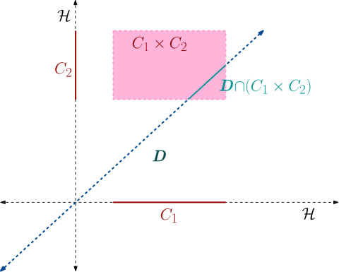
Fig. 1: Visualization of the product space for $\mathcal{H}=\mathbb{R}$ and $m=2$. Our algorithm produces iterates $\boldsymbol{x}_{t}$ which are always inside the shaded constraint set, and their averages $A^{*}A\boldsymbol{x}_{t}$ are always on the diagonal subspace $\boldsymbol{D}$. The solid segment where $C_{1}\times C_{2}$ and $\boldsymbol{D}$ intersect corresponds precisely to our split feasibility constraint via Proposition 2.1.

Proposition 2.1 provides a decomposition of the split feasibility constraint $\bigcap_{i\in I}C_{i}$ in terms of two simpler sets $\boldsymbol{D}$ and $\bigtimes_{i\in I}C_{i}$. This yields a product space reformulation of (1)

$$\underset{\boldsymbol{x}\in\bigtimes_{i\in I}C_{i}}{\text{minimize}}\;\;f(A\boldsymbol{x})+\iota_{\boldsymbol{D}}(\boldsymbol{x}).$$ (14)

The constraints $\boldsymbol{D}$ and $\bigtimes_{i\in I}C_{i}$ are simpler in the sense that, even in our restricted computational setting, we can compute operators to enforce them. In particular, the projection onto $\boldsymbol{D}$ is computed by simply repeating the average of all components in every component $\text{\rm Proj}\,_{\boldsymbol{D}}\boldsymbol{x}=A^{*}(\sum_{i\in I}\omega_{i}\boldsymbol{x}^{i})$. Critically, this operation is cheap, so one can actually evaluate the gradient $\nabla\text{\rm dist}\,_{\boldsymbol{D}}^{2}/2=\text{Id}-\text{\rm Proj}\,_{D}$ even though it involves a projection. The constraint $\bigtimes_{i\in I}C_{i}$ is readily processed using the following property.

Fact 2.2

Let $(C_{i})_{i\in I}$ be a collection of nonempty compact convex subsets of $\mathcal{H}$. Then

$$(\forall\boldsymbol{x}\in\boldsymbol{\mathcal{H}})\quad\operatorname{LMO}_{(\bigtimes_{i\in I}C_{i})}(\boldsymbol{x})=(\operatorname{LMO}_{C_{1}}\boldsymbol{x}^{1},\ldots,\operatorname{LMO}_{C_{m}}\boldsymbol{x}^{m}).$$ (15)

In particular, to evaluate an LMO for the product $\bigtimes_{i\in I}C_{i}$, it suffices to evaluate the individual operators $(\operatorname{LMO}_{i})_{i\in I}$ once.

With these ideas in mind, let us introduce the penalized function

$$F_{\lambda}\colon\boldsymbol{\mathcal{H}}\to\mathbb{R}\colon\boldsymbol{x}\mapsto f(A\boldsymbol{x})+\lambda\frac{1}{2}\text{\rm dist}\,_{\boldsymbol{D}}^{2}(\boldsymbol{x}),$$ (16)

which, for every $\lambda\geq 0$, is $(L_{f}+\lambda)$-smooth (cf. Fact 1.1). We observe that for every penalty parameter $\lambda_{t}\geq 0$, even under our restricted computational setting, the following relaxation of (14) is still tractable with the vanilla CG algorithm

$$\underset{\boldsymbol{x}\in\bigtimes_{i\in I}C_{i}}{\text{minimize}}\;\;F_{\lambda_{t}}(\boldsymbol{x}).$$ (17)

Indeed, vanilla CG requires the ability to compute the gradient of the objective function and the LMO of the constraint. Computing $\nabla F_{\lambda}=\nabla f+\lambda(\text{Id}-\text{\rm Proj}\,_{\boldsymbol{D}})$ amounts to one evaluation of $\nabla f$, computing one average, and some algebraic manipulations. By promoting membership of $\boldsymbol{D}$ via the objective function, we are left with the LMO-amenable constraint $\bigtimes_{i\in I}C_{i}$.

The core idea of our algorithm is, at each iteration $t\in\mathbb{N}$, to perform one Frank-Wolfe step to the relaxed subproblem (17). Then, between iterations, we update the objective function in (17) via $\lambda_{t}$ to promote feasibility. Although (17) is a relaxation of the intractable problem (14), taking $\lambda_{t}\to\infty$ suffices to show convergence in F-W gap (and primal gap, in the convex case) to solutions of (14) and hence (1); this is substantiated in Sections 2.2.2 and 3. For every $\boldsymbol{x}\in\boldsymbol{\mathcal{H}}$, the $i$th component of the gradient is given by $\nabla F_{\lambda}(\boldsymbol{x})^{i}=\nabla f(A\boldsymbol{x})+\lambda(\boldsymbol{x}^{i}-A\boldsymbol{x})$. So, a CG step applied to (17) yields Algorithm 1. While Section 3 contains the precise schedules for Lines 3 and 4, the parameters behave like $(\lambda_{t},\gamma_{t})=(\mathcal{O}(\ln t),\mathcal{O}(1/\sqrt{t}))$.

Algorithm 1 Split conditional gradient (SCG) algorithm

0:  Smooth function $f$, weights $\{\omega_{i}\}_{i\in I}\subset\left]0,1\right]$ such that $\sum_{i\in I}\omega_{i}=1$, point $\boldsymbol{x}_{0}\in\bigtimes_{i\in I}C_{i}$

1:  $x_{0}\leftarrow\sum_{i\in I}\omega_{i}\boldsymbol{x}_{0}^{i}$

2:  for $t=0,1$ to $\dotsc$ do

3:     Choose penalty parameter $\lambda_{t}\in\left]0,+\infty\right[$

4:     Choose step size $\gamma_{t}\in\left]0,1\right]$

5:     $g_{t}\leftarrow\nabla f(x_{t})$ # COMMENTStore $\nabla f(A\boldsymbol{x}_{t})$ for CG step on (17)

6:     for $i=1$ to $m$ do

7:        $\boldsymbol{v}_{t}^{i}\leftarrow\operatorname{LMO}_{i}(g_{t}+\lambda_{t}(\boldsymbol{x}_{t}^{i}-x_{t}))$ # COMMENTLMO applied to $\nabla F_{\lambda_{t}}(\boldsymbol{x}_{t})^{i}$

8:        $\boldsymbol{x}_{t+1}^{i}\leftarrow\boldsymbol{x}_{t}^{i}+\gamma_{t}(\boldsymbol{v}_{t}^{i}-\boldsymbol{x}_{t}^{i})$ # COMMENTCG step in $i$th component

9:     end for

10:     $x_{t+1}\leftarrow\sum_{i\in I}\omega_{i}\boldsymbol{x}_{t+1}^{i}$ # COMMENTApproximate solution by averaging

11:  end for

CG-based algorithms possess the advantage that, at every iteration, the iterates are feasible (i.e., for (11), $x_{t}\in C$). Our approach inherits this familiar property; however, since we solve a product space relaxation, $\boldsymbol{x}_{t}\in\bigtimes_{i\in I}C_{i}$ and hence, for every $i\in I$, the $i$th component of our sequence is feasible for the $i$th constraint, i.e., $(\boldsymbol{x}_{t}^{i})_{t\in\mathbb{N}}\in C_{i}$. Importantly, this does not guarantee that any subcomponent $\boldsymbol{x}_{t}^{i}$ resides in $\bigcap_{i\in I}C_{i}$, so they are not feasible for the splitting problem (1); feasibility in $\bigcap_{i\in I}C_{i}$ is acquired “in the limit”, by showing that $\boldsymbol{x}_{t}\in\bigtimes_{i\in I}C_{i}$ and $\text{\rm dist}\,_{\boldsymbol{D}}(\boldsymbol{x}_{t})\to 0$ (proven in Section 3).

In practice, one needs a route to construct an approximate solution to (1) in $\mathcal{H}$ from an iterate of Algorithm 1 in the product space $\boldsymbol{\mathcal{H}}$. Instead of taking a component, we use the average computed in Line 10 as our approximate solution, since

$$(\forall\boldsymbol{x}\in\boldsymbol{\mathcal{H}})\quad\quad\boldsymbol{x}\in\boldsymbol{D}\cap\bigtimes_{i\in I}C_{i}\quad\Rightarrow\quad A\boldsymbol{x}\in\bigcap_{i\in I}C_{i}$$ (18)

is a strict implication. Hence the condition $A\boldsymbol{x}\in\bigcap_{i\in I}C_{i}$ is easier to satisfy than $\boldsymbol{x}\in\boldsymbol{D}\cap\bigtimes_{i\in I}C_{i}$ (see also Sec. 2.2.1).

Remark 2.3

If we have only $m=1$ set constraint, then $A=\text{Id}$, and $\mathcal{H}=\boldsymbol{\mathcal{H}}=\boldsymbol{D}$, so at every iteration $t\in\mathbb{N}$, $F_{\lambda_{t}}=f(x)$. Therefore, the classical CG algorithm is a special case of Algorithm 1.

2.2 Analysis

Here we gather analytical results pertaining to our algorithm, the geometry of our product-space construction, and how our relaxed problem relates to other classical problems in optimization. While these results are interesting in their own right, many are also used to show convergence in Section 3.

2.2.1 Geometry (and tractability) of penalty functions on the Cartesian product

As seen in Section 2.1, Algorithm 1 promotes split feasibility by, at every iteration $t\in\mathbb{N}$, requiring that $\boldsymbol{x}_{t}\in\bigtimes_{i\in I}C_{i}$ and penalizing the distance from $\boldsymbol{x}_{t}$ to $\boldsymbol{D}$. However, as seen in (18), $\text{\rm dist}\,_{\boldsymbol{D}}(\boldsymbol{x}_{t})=0$ is a sufficient (but not necessary) condition to acquire a feasible average $A\boldsymbol{x}_{t}\in\bigcap_{i\in I}C_{i}$; see Fig. 2. In this section, we present a penalty function which precisely characterizes this condition. Via a simple geometric argument based on the projection theorem, we guarantee that although utilizing this penalty is not computationally tractable, it is nonetheless minimized when $\text{\rm dist}\,_{\boldsymbol{D}}$ vanishes. These results also further substantiate the claim that $\boldsymbol{x}\in\boldsymbol{D}\cap\bigtimes_{i\in I}C_{i}$ is a stricter condition than $A\boldsymbol{x}\in\bigcap_{i\in I}C_{i}$, which is our motivation to use the average in Line 10 of Algorithm 1 as our approximate solution to (1).

Proposition 2.4

Let $(C_{i})_{i\in I}$ be a collection of nonempty closed convex subsets of $\mathcal{H}$, let $\boldsymbol{D}\subset\boldsymbol{\mathcal{H}}$ denote the diagonal subspace, and set

$$d\colon\boldsymbol{\mathcal{H}}\to\left]-\infty,+\infty\right]\colon\boldsymbol{x}\mapsto\sum_{i\in I}\omega_{i}\text{\rm dist}\,^{2}_{C_{i}}(A\boldsymbol{x}).$$ (19)

Then, for every $\boldsymbol{x}\in\boldsymbol{\mathcal{H}}$, the following are equivalent.

1. $d(\boldsymbol{x})=0$.

2. $A\boldsymbol{x}\in\bigcap_{i\in I}C_{i}$.

3. $\text{\rm Proj}\,_{\boldsymbol{D}}(\boldsymbol{x})\in\bigtimes_{i\in I}C_{i}$.

Proof. (i)$\Rightarrow$(ii): For every $i\in I$, $0\leq\omega_{i}\text{\rm dist}\,^{2}_{C_{i}}(A\boldsymbol{x})\leq d(\boldsymbol{x})=0$. Since $\omega_{i}>0$, it follows that $\text{\rm dist}\,^{2}_{C_{i}}(A\boldsymbol{x})=0$ and hence $A\boldsymbol{x}\in C_{i}$.

(ii)$\Rightarrow$(iii): By applying $A^{*}$ to the inclusion (ii), (6) implies that

$$\text{\rm Proj}\,_{\boldsymbol{D}}\boldsymbol{x}=A^{*}A\boldsymbol{x}\in A^{*}\bigcap_{i\in I}C_{i}=\left\{{(x,\ldots,x)\in\boldsymbol{\mathcal{H}}}~{}\left|~{}{x\in\bigcap_{i\in I}C_{i}}\right.\right\}.$$ (20)

So, by Proposition 2.1, $\text{\rm Proj}\,_{\boldsymbol{D}}\boldsymbol{x}\in\left\{{\boldsymbol{x}\in\boldsymbol{\mathcal{H}}}~{}\left|~{}{\boldsymbol{x}\in\boldsymbol{D}\cap\bigtimes_{i\in I}C_{i}}\right.\right\}\subset\bigtimes_{i\in I}C_{i}$.

(iii)$\Rightarrow$(i): We begin by observing that

$$\text{\rm Proj}\,_{\bigtimes_{i\in I}C_{i}}(\text{\rm Proj}\,_{\boldsymbol{D}}\boldsymbol{x})=\underset{\boldsymbol{c}\in\bigtimes_{i\in I}C_{i}}{{\text{\rm Argmin}}\,}\|\boldsymbol{c}-A^{*}A\boldsymbol{x}\|_{\boldsymbol{\mathcal{H}}}^{2}=\underset{\boldsymbol{c}\in\bigtimes_{i\in I}C_{i}}{{\text{\rm Argmin}}\,}\sum_{i\in I}\omega_{i}\|\boldsymbol{c}^{i}-A\boldsymbol{x}\|_{\mathcal{H}}^{2}$$ (21)

is a separable problem whose solution is $\left(\text{\rm Proj}\,_{C_{1}}(A\boldsymbol{x}),\ldots,\text{\rm Proj}\,_{C_{m}}(A\boldsymbol{x})\right)$. Therefore,

$$d(\boldsymbol{x})=\sum_{i\in I}\omega_{i}\|A\boldsymbol{x}-\text{\rm Proj}\,_{C_{i}}(A\boldsymbol{x})\|_{\mathcal{H}}^{2}=\|\text{\rm Proj}\,_{\boldsymbol{D}}\boldsymbol{x}-\text{\rm Proj}\,_{\bigtimes_{i\in I}C_{i}}(\text{\rm Proj}\,_{\boldsymbol{D}}\boldsymbol{x})\|_{\boldsymbol{\mathcal{H}}}^{2}.$$ (22)

Since $\text{\rm Proj}\,_{\boldsymbol{D}}(\boldsymbol{x})=\text{\rm Proj}\,_{\bigtimes_{i\in I}C_{i}}(\text{\rm Proj}\,_{\boldsymbol{D}}\boldsymbol{x})$, we conclude $d(\boldsymbol{x})=0$. $\square$

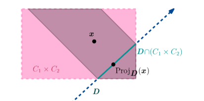
Fig. 2: Zoomed view of Fig. 1. The darker shaded area is the collection of points $\boldsymbol{x}\in\bigtimes_{i\in I}C_{i}$ for which $\text{\rm Proj}\,_{\boldsymbol{D}}(\boldsymbol{x})$ remains in $\bigtimes_{i\in I}C_{i}$. By Proposition 2.4, this is the set of points satisfying $A\boldsymbol{x}\in\bigcap_{i\in I}C_{i}$. This exemplifies that the implication (18) is strict.

Since we do not assume the ability to project onto the sets $(C_{i})_{i\in I}$, evaluating $\nabla d=2\sum_{i\in I}\omega_{i}(\text{Id}-\text{\rm Proj}\,_{C_{i}})$ is not possible. Therefore, replacing $F_{\lambda}$ in (17) with the composite function $f(A\boldsymbol{x})+\lambda d(\boldsymbol{x})$ is not tractable with a vanilla CG-based approach. However, $d$ is closely related to our penalty function $\text{\rm dist}\,^{2}_{\boldsymbol{D}}$ via the following result.

Corollary 2.5

In the setting of Proposition 2.4, let $\boldsymbol{x}\in\bigtimes_{i\in I}C_{i}$, set $\boldsymbol{y}=\text{\rm Proj}\,_{\boldsymbol{D}}\boldsymbol{x}$ and set $\boldsymbol{p}=\text{\rm Proj}\,_{(\bigtimes_{i\in I}C_{i})}(\boldsymbol{y})$. Then

$$d(\boldsymbol{x})=\text{\rm dist}\,_{\boldsymbol{D}}^{2}(\boldsymbol{x})-\|\boldsymbol{x}-\boldsymbol{p}\|^{2}+2\underbrace{{\langle{{\boldsymbol{x}-\boldsymbol{p}}\mid{\boldsymbol{y}-\boldsymbol{p}}}\rangle}}_{\leq 0}.$$ (23)

In consequence, $0\leq d(\boldsymbol{x})\leq\text{\rm dist}\,_{\boldsymbol{D}}^{2}(\boldsymbol{x})$.

Proof. Follows from Lemma 2.12 and Theorem 3.16 of [28]. $\square$

Since the iterates of Algorithm 1 always reside in $\bigtimes_{i\in I}C_{i}$, Corollary 2.5 reinforces our choice of $A\boldsymbol{x}_{t}$ as our approximate solution of (1). Firstly, its implication that $\text{\rm dist}\,^{2}_{\boldsymbol{D}}(\boldsymbol{x})=0\Rightarrow d(\boldsymbol{x})=0$ underlines the observation from (18) that $A\boldsymbol{x}_{t}\in\bigcap_{i\in I}C_{i}$ is easier to satisfy than $\boldsymbol{x}\in\boldsymbol{D}\cap\bigtimes_{i\in I}C_{i}$. Furthermore, by characterizing the gap between $d$ and $\text{\rm dist}\,_{\boldsymbol{D}}^{2}$, we see that there are plenty of points for which the inequality between $d$ and $\text{\rm dist}\,_{\boldsymbol{D}}^{2}$ is strict, e.g., those $\boldsymbol{x}\in\bigtimes_{i\in I}C_{i}$ for which $\boldsymbol{x}\neq\boldsymbol{p}$ (see also Fig. 2). Due to this strictness, $d(\boldsymbol{x}_{t})$ may vanish far before $\text{\rm dist}\,_{\boldsymbol{D}}^{2}(\boldsymbol{x}_{t})$ vanishes over the iterations of Algorithm 1. This is consistent with our preliminary numerical observations that $A\boldsymbol{x}_{t}\in\bigcap_{i\in I}C_{i}$ often occurs before $\text{\rm dist}\,^{2}_{\boldsymbol{D}}(\boldsymbol{x}_{t})$ vanishes.

Remark 2.6

The function $g\colon\boldsymbol{x}\mapsto\text{\rm dist}\,_{\bigcap_{i\in I}C_{i}}^{2}(A\boldsymbol{x})=\|\text{\rm Proj}\,_{\boldsymbol{D}}\boldsymbol{x}-\text{\rm Proj}\,_{\boldsymbol{D}\cap(C_{1}\times C_{2})}\boldsymbol{x}\|^{2}$ is also a natural penalty to consider, although evaluating $\nabla g=2A^{*}(\text{Id}-\text{\rm Proj}\,_{\bigcap_{i\in I}C_{i}})(A\boldsymbol{x})$ involves computing an intractable projection. While, for every $\boldsymbol{x}\in\mathcal{H}$, $g$ and $d$ (see (19)) have the order

$$d(\boldsymbol{x})=\sum_{i\in I}\omega_{i}\inf_{c\in C_{i}}\|A\boldsymbol{x}-c\|^{2}\leq\sum_{i\in I}\omega_{i}\inf_{c\in\bigcap_{i\in I}C_{i}}\|A\boldsymbol{x}-c\|^{2}=g(\boldsymbol{x}),$$ (24)

there is no general ordering between $g$ and our penalty $\text{\rm dist}\,_{\boldsymbol{D}}^{2}$ for $\dim(\mathcal{H})\geq 2$. However, they are related in the following geometric sense

$$g(\boldsymbol{x})+\text{\rm dist}\,_{\boldsymbol{D}}^{2}(\boldsymbol{x})=\sum_{i\in I}\omega_{i}\|x^{i}-P_{\bigcap_{i\in I}C_{i}}(Ax)\|^{2}+\underbrace{2{\langle{{A^{*}P_{\bigcap_{i\in I}C_{i}}(Ax)-A^{*}Ax}\mid{x-A^{*}Ax}}\rangle}}_{=0}.$$ (25)

Since the lefthand and righthand vectors in the scalar product are in $\boldsymbol{D}$ and $\boldsymbol{D}^{\perp}$ respectively, $g$ and $\text{\rm dist}\,_{\boldsymbol{D}}^{2}$ describe the squared magnitude of two orthogonal vectors.

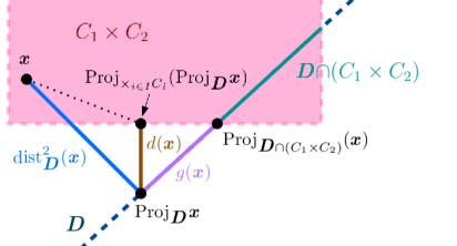
Fig. 3: Zoomed view of Fig. 1 displaying geometric relationships between $\text{\rm dist}\,_{\boldsymbol{D}}^{2}$, $d$, and $g$ (see (22) and Remark 2.6). This shows a feasible point $\boldsymbol{x}\in\bigtimes_{i\in I}C_{i}$ and several vectors whose squared magnitude are equal to the given labels. Corollary 2.5 describes the relative magnitude of $\text{\rm dist}\,^{2}_{\boldsymbol{D}}$ and $d$, as well as the obtuse angle between $\boldsymbol{x}$, $\text{\rm Proj}\,_{\bigtimes_{i\in I}C_{i}}(\text{\rm Proj}\,_{\boldsymbol{D}}\boldsymbol{x})$, and $\text{\rm Proj}\,_{\boldsymbol{D}}$. Remark 2.6 describes the orthogonality seen in the angle between $\boldsymbol{x}$, $\text{\rm Proj}\,_{\boldsymbol{D}}\boldsymbol{x}$, and $\text{\rm Proj}\,_{\boldsymbol{D}\cap\bigtimes_{i\in I}C_{i}}(\boldsymbol{x})$. We also see $\text{\rm Proj}\,_{\boldsymbol{D}\cap\bigtimes_{i\in I}C_{i}}\boldsymbol{x}=\text{\rm Proj}\,_{\boldsymbol{D}\cap\bigtimes_{i\in I}C_{i}}(\text{\rm Proj}\,_{\boldsymbol{D}}\boldsymbol{x})$, which holds in general [28, Prop. 24.18].

2.2.2 Interpolating constraints: From the Minkowski sum to the intersection

This section presents an analysis of how our subproblem (17) changes with the parameter $\lambda$. In addition to their utility in Section 3 to prove that our sequence of relaxations (17) actually solves the correct problem (14), the results in this section show that (17) connects two classical problems in optimization.

From a certain perspective, (17) “interpolates” from the following problem (when $\lambda=0$) over the Minkowski sum

$$\underset{x\in\sum_{i\in I}\omega_{i}C_{i}}{\text{minimize}}\;\;f(x),\quad\text{where}\quad\sum_{i\in I}\omega_{i}C_{i}=\left\{{\sum_{i\in I}\omega_{i}c^{i}}~{}\left|~{}{(\forall i\in I)\;\;c^{i}\in C_{i}}\right.\right\},$$ (26)

to the splitting problem (1) (when $\lambda\nearrow+\infty$). We shall make this latter observation precise via several notions of convergence in Proposition 2.12.

Remark 2.7

While this article is predominantly focused on (1), it is worth noting that, when $\lambda=0$, the problems (17) and (26) coincide in the sense that, for every solution $\boldsymbol{x}^{*}$ of (17), $A\boldsymbol{x}^{*}$ solves (26) (and for every solution $\sum_{i\in I}\omega_{i}x^{i}$ of (26), $(x^{i})_{i\in I}$ solves (17)). Therefore, Fact 2.2 leads to a Frank-Wolfe approach to solving (26). The Minkowski sum constraint arises in Bayesian learning, placement problems, and robot motion planning [29, 30, 31, 32].

We begin with the following observations about how $F_{\lambda}$ relates as $\lambda$ varies.

Lemma 2.8

Let $f\colon\mathcal{H}\to\mathbb{R}$, let $\lambda,\Delta\in\mathbb{R}$, let $\boldsymbol{D}\subset\boldsymbol{\mathcal{H}}$ be nonempty, and set $F_{\lambda}\colon\boldsymbol{x}\mapsto f(A\boldsymbol{x})+\lambda\text{\rm dist}\,_{\boldsymbol{D}}^{2}(\boldsymbol{x})/2$. Then,

$$(\forall\boldsymbol{x}\in\boldsymbol{\mathcal{H}})\quad F_{\lambda}(\boldsymbol{x})=F_{\lambda+\Delta}(\boldsymbol{x})-\Delta\frac{1}{2}\text{\rm dist}\,_{\boldsymbol{D}}^{2}(\boldsymbol{x}).$$ (27)

In consequence, if $\Delta\geq 0$, then $F_{\lambda}(\boldsymbol{x})\leq F_{\lambda+\Delta}(\boldsymbol{x})$ and $\inf F_{\lambda}(\bigtimes_{i\in I}C_{i})\leq\inf F_{\lambda+\Delta}(\bigtimes_{i\in I}C_{i})$.

Proof. $F_{\lambda}(\boldsymbol{x})=f(A\boldsymbol{x})+(\lambda+\Delta)\text{\rm dist}\,_{\boldsymbol{D}}^{2}(\boldsymbol{x})/2-\Delta\text{\rm dist}\,_{\boldsymbol{D}}^{2}(\boldsymbol{x})/2=F_{\lambda+\Delta}(\boldsymbol{x})-\Delta\text{\rm dist}\,_{\boldsymbol{D}}^{2}(\boldsymbol{x})/2$. $\square$

Next, we show that the optimal value of (17) is sandwiched between that of the splitting problem (1) and the Minkowski sum problem (26).

Proposition 2.9

Let $f\colon\mathcal{H}\to\mathbb{R}$, let $\lambda\geq 0$, let $\boldsymbol{D}\subset\boldsymbol{\mathcal{H}}$ be nonempty, set $F_{\lambda}\colon\boldsymbol{x}\mapsto f(A\boldsymbol{x})+\lambda\text{\rm dist}\,_{\boldsymbol{D}}^{2}(\boldsymbol{x})/2$, and let $(C_{i})_{i\in I}$ be a collection of nonempty compact convex subsets of $\mathcal{H}$ such that $\bigcap_{i\in I}C_{i}\neq\varnothing$. Then

$$\inf_{x\in\bigcap_{i\in I}C_{i}}f(x)\geq\inf_{\boldsymbol{x}\in\bigtimes_{i\in I}C_{i}}F_{\lambda}\geq\inf_{x\in\sum_{i\in I}\omega_{i}C_{i}}f(x).$$ (28)

Proof. To show the first inequality, we note that for every $\boldsymbol{x}\in\boldsymbol{D}$, $\text{\rm dist}\,_{\boldsymbol{D}}^{2}(\boldsymbol{x})=0$, so using the product space formulation (14) of (1),

$$\inf_{x\in\bigcap_{i\in I}C_{i}}f(x)=\inf_{\boldsymbol{x}\in\boldsymbol{D}\cap\bigtimes_{i\in I}C_{i}}f(A\boldsymbol{x})+\frac{\lambda}{2}\text{\rm dist}\,_{\boldsymbol{D}}^{2}(\boldsymbol{x})\geq\inf_{\boldsymbol{x}\in\bigtimes_{i\in I}C_{i}}F_{\lambda}(\boldsymbol{x}).$$ (29)

The second inequality follows from the observation that (26) coincides with $\inf_{\boldsymbol{x}\in\bigtimes_{i\in I}C_{i}}F_{0}(\boldsymbol{x})$, so by Lemma 2.8 we have $\inf_{\boldsymbol{x}\in\bigtimes_{i\in I}C_{i}}F_{\lambda}(\boldsymbol{x})\geq\inf_{\boldsymbol{x}\in\bigtimes_{i\in I}C_{i}}F_{0}(\boldsymbol{x})$. $\square$

It turns out that, for an increasing sequence of penalty parameters $(\lambda_{n})_{n\in\mathbb{N}}$, the ordering of Proposition 2.9 is preserved if we only consider the optimal values of $f$ (instead of $F_{\lambda}$). Intuitively, the order is reversed when we compare optimal values of the penalty $\text{\rm dist}\,_{\boldsymbol{D}}^{2}$.

Corollary 2.10

Let $f\colon\mathcal{H}\to\mathbb{R}$, let $\boldsymbol{D}\subset\boldsymbol{\mathcal{H}}$ be nonempty, set $F_{\lambda}\colon\boldsymbol{x}\mapsto f(A\boldsymbol{x})+\lambda\text{\rm dist}\,_{\boldsymbol{D}}^{2}(\boldsymbol{x})/2$, and let $(C_{i})_{i\in I}$ be a collection of nonempty compact convex subsets of $\mathcal{H}$ such that $\bigcap_{i\in I}C_{i}\neq\varnothing$. Suppose that $(\lambda_{t})_{t\in\mathbb{N}}$ is an increasing sequence of real numbers and, for every $t\in\mathbb{N}$, let $\boldsymbol{x}_{t}^{*}$ be a minimizer of $F_{\lambda_{t}}$ over $\bigtimes_{i\in I}C_{i}$. Then

$$\inf_{x\in\bigcap_{i\in I}C_{i}}f(x)\geq f\left(A\boldsymbol{x}_{t+1}^{*}\right)\geq f\left(A\boldsymbol{x}_{t}^{*}\right)\geq\inf_{x\in\sum_{i\in I}\omega_{i}C_{i}}f\left(x\right).$$ (30)

If $\boldsymbol{z}\in{\text{\rm Argmin}}\,_{\boldsymbol{x}\in\bigtimes_{i\in I}C_{i}}f\left(A\boldsymbol{x}\right)$ (i.e., $A\boldsymbol{z}$ solves (26)), then

$$0\leq\text{\rm dist}\,_{\boldsymbol{D}}^{2}(\boldsymbol{x}_{t+1}^{*})\leq\text{\rm dist}\,_{\boldsymbol{D}}^{2}(\boldsymbol{x}_{t}^{*})\leq\text{\rm dist}\,_{\boldsymbol{D}}^{2}(\boldsymbol{z}).$$ (31)

Proof. Follows from Lemma 1.2 and Proposition 2.9. $\square$

The following example demonstrates that the penalty sequence $(\lambda_{t})_{t\in\mathbb{N}}$ may need to tend to $+\infty$ in order for the solutions of (17) and (1) to coincide.

Example 2.11

Set $\mathcal{H}=\mathbb{R}$, set $f=\|x\|^{2}/2$, let $z\geq 0$, set $C_{1}=\{z\}$, and set $C_{2}=[-z-1,z+1]$. Clearly, $z={\text{\rm Argmin}}\,_{x\in C_{1}\cap C_{2}}f(x)$. However, it is straightforward to verify that, for every $\lambda\geq 0$, $\boldsymbol{x}^{*}_{\lambda}=((\lambda-1)z/(1+\lambda),z)$ is the unique minimizer of $F_{\lambda}$ over $C_{1}\times C_{2}$. Since $A\boldsymbol{x}^{*}_{\lambda}=\lambda z/(1+\lambda)\neq z$, the solutions of (17) and (1) (via (14)) do not coincide for finite $\lambda$; taking $\lambda\to+\infty$ implies $A\boldsymbol{x}^{*}_{\lambda}\to z$.

The following result establishes three notions of convergence (see Definition 1.3) relating the problems (17) and (1) (via its equivalent product space formulation (14)). For this result, we rely on the fact that every constrained optimization problem can be described using a single objective function via the use of indicator functions.

Proposition 2.12

Let $f\colon\mathcal{H}\to\mathbb{R}$, let $(C_{i})_{i\in I}$ be a collection of nonempty compact convex subsets of $\mathcal{H}$ such that $\bigcap_{i\in I}C_{i}\neq\varnothing$, and let $\boldsymbol{D}$ denote the diagonal subspace of $\boldsymbol{\mathcal{H}}$. Suppose that $(\lambda_{t})_{t\in\mathbb{N}}\to+\infty$ and, for every $t\in\mathbb{N}$, set $\boldsymbol{f}_{t}=f\circ A+\lambda_{t}\text{\rm dist}\,_{\boldsymbol{D}}^{2}/2+\iota_{\bigtimes_{i\in I}C_{i}}$. Then the following hold.

1. $\boldsymbol{f}_{t}$ converges pointwise to $f\circ A+\iota_{\boldsymbol{D}\cap\bigtimes_{i\in I}C_{i}}$.

2. Suppose $\mathcal{H}=\mathbb{R}^{n}$. Then $\boldsymbol{f}_{t}$ converges epigraphically to $f\circ A+\iota_{\boldsymbol{D}\cap\bigtimes_{i\in I}C_{i}}$.

3. Suppose $\mathcal{H}=\mathbb{R}^{n}$ and $f$ is convex. Then $\partial\boldsymbol{f}_{n}$ converges graphically to $\partial(f\circ A+\iota_{\boldsymbol{D}\cap\bigtimes_{i\in I}C_{i}})$.

Proof. Since

$$\iota_{\bigtimes_{i\in I}C_{i}}+\iota_{D}=\iota_{D\cap\bigtimes_{i\in I}C_{i}},$$ (32)

it suffices to show that $\lambda_{t}\text{\rm dist}\,_{\boldsymbol{D}}^{2}/2$ converges to $\iota_{D}$ under each notion of convergence.
(i): Let $\boldsymbol{x}\in\boldsymbol{\mathcal{H}}$. If $\boldsymbol{x}\in\boldsymbol{D}$, then for every $n\in\mathbb{N}$, $\lambda_{t}\text{\rm dist}\,_{\boldsymbol{D}}^{2}(\boldsymbol{x})/2=0=\iota_{\boldsymbol{D}}(\boldsymbol{x})$. On the other hand, if $\boldsymbol{x}\not\in\boldsymbol{D}$, then $0<\lambda_{t}\text{\rm dist}\,_{\boldsymbol{D}}^{2}(\boldsymbol{x})/2\to+\infty=\iota_{D}(\boldsymbol{x})$.
(ii): Let $\boldsymbol{x}\in\boldsymbol{\mathcal{H}}$. By [26, Proposition 7.2], it suffices to show both of the following.

$$\text{For some sequence}\;(\boldsymbol{x}_{t})_{t\in\mathbb{N}}\text{ converging to } \boldsymbol{x},\quad\lim\sup_{t\in\mathbb{N}}\frac{\lambda_{t}}{2}\text{\rm dist}\,_{\boldsymbol{D}}^{2}(\boldsymbol{x}_{t})\leq\iota_{\boldsymbol{D}}(\boldsymbol{x}).$$ (33)

$$\text{For every sequence}\;(\boldsymbol{x}_{t})_{t\in\mathbb{N}}\text{ converging to } \boldsymbol{x},\quad\lim\inf_{t\in\mathbb{N}}\frac{\lambda_{t}}{2}\text{\rm dist}\,_{\boldsymbol{D}}^{2}(\boldsymbol{x}_{t})\geq\iota_{\boldsymbol{D}}(\boldsymbol{x}).$$ (34)

To realize (33), we consider the constant sequence $(\boldsymbol{x}_{t})_{t\in\mathbb{N}}\equiv\boldsymbol{x}$. By (i),

$$\lim\sup_{t\in\mathbb{N}}\lambda_{t}\text{\rm dist}\,_{\boldsymbol{D}}^{2}(\boldsymbol{x}_{t})/2=\lim_{t\in\mathbb{N}}\lambda_{t}\text{\rm dist}\,_{\boldsymbol{D}}^{2}(\boldsymbol{x})/2=\iota_{\boldsymbol{D}}(\boldsymbol{x}),$$ (35)

so this is always satisfied with equality. To show (34), let $(\boldsymbol{x}_{t})_{t\in\mathbb{N}}$ be a sequence converging to $\boldsymbol{x}$. If $\boldsymbol{x}\in\boldsymbol{D}$, then since $\text{\rm dist}\,_{\boldsymbol{D}}^{2}\geq 0$ and $\iota_{\boldsymbol{D}}(\boldsymbol{x})=0$, (34) holds. Otherwise, if $\boldsymbol{x}\not\in\boldsymbol{D}$, then there exists a radius $\varepsilon>0$ such that $B(\boldsymbol{x};\varepsilon)\cap\boldsymbol{D}=\varnothing$. Since $\text{\rm dist}\,_{\boldsymbol{D}}^{2}$ is continuous and only vanishes on $\boldsymbol{D}$, we know $\eta:=\inf_{\boldsymbol{y}\in B(\boldsymbol{x};\varepsilon/2)}\text{\rm dist}\,_{\boldsymbol{D}}^{2}(\boldsymbol{y})/2>0$. Therefore, since $\boldsymbol{x}_{t}\to\boldsymbol{x}$, we have that, for some $N\in\mathbb{N}$, $n>N$ implies that $\boldsymbol{x}_{t}\in B(\boldsymbol{x};\varepsilon/2)$, hence

$$\frac{\lambda_{t}}{2}\text{\rm dist}\,_{\boldsymbol{D}}^{2}(\boldsymbol{x}_{t})\geq\lambda_{t}\eta\to+\infty.$$ (36)

In particular, $\lim_{t\in\mathbb{N}}\lambda_{t}\text{\rm dist}\,_{\boldsymbol{D}}^{2}(\boldsymbol{x}_{t})/2=+\infty=\iota_{\boldsymbol{D}}(\boldsymbol{x})$ so we are done.
(iii): Follows from (ii) and Attouch’s Theorem [26, Theorem 12.35]. $\square$

In general, the functions in Proposition 2.12 do not converge uniformly. In spite of this, it turns out that one can nonetheless commute the limit with an infimum, hence showing that the optimal values of our subproblems (17) converge to the optimal value of (1).

Proposition 2.13

Let $f\colon\mathcal{H}\to\mathbb{R}$, let $(C_{i})_{i\in I}$ be a collection of nonempty compact convex subsets of $\mathcal{H}$, let $\boldsymbol{D}$ denote the diagonal subspace of $\boldsymbol{\mathcal{H}}$, and for every $\lambda\geq 0$, set $F_{\lambda}\colon\boldsymbol{x}\mapsto f(A\boldsymbol{x})+\lambda\text{\rm dist}\,_{\boldsymbol{D}}^{2}(\boldsymbol{x})/2$. Suppose that $(\lambda_{n})_{n\in\mathbb{N}}\nearrow+\infty$. Then

$$\lim_{t\to+\infty}\left(\inf_{\boldsymbol{x}\in\bigtimes_{i\in I}C_{i}}F_{\lambda_{t}}(\boldsymbol{x})\right)\to\inf_{\boldsymbol{x}\in\bigtimes_{i\in I}C_{i}}\left(\lim_{t\to\infty}F_{\lambda_{t}}(\boldsymbol{x})\right)=\inf_{x\in\bigcap_{i\in I}C_{i}}f(x).$$ (37)

Proof. First, we point out that the equality in (37) follows from Proposition 2.12 and the fact that the minimal values of (1) and (14) coincide. Let $\mu<\inf_{x\in\bigcap_{i\in I}C_{i}}f(x)=\inf_{\boldsymbol{x}\in\bigtimes_{i\in I}C_{i}}f(A\boldsymbol{x})+\iota_{\boldsymbol{D}}(\boldsymbol{x})$. By Proposition 2.12, for every $\boldsymbol{x}\in\bigtimes_{i\in I}C_{i}$, $\lim_{t\to\infty}F_{\lambda_{t}}(\boldsymbol{x})=f(A\boldsymbol{x})+\iota_{\boldsymbol{D}}(\boldsymbol{x})>\mu$. Since $\bigtimes_{i\in I}C_{i}$ is compact, for $t\in\mathbb{N}$ sufficiently large, $\inf_{\boldsymbol{x}\in\bigtimes_{i\in I}C_{i}}F_{\lambda_{t}}(\boldsymbol{x})\geq\mu$, which implies (via Proposition 2.9 for the second inequality)

$$\mu\leq\lim_{t\to\infty}\left(\inf_{\boldsymbol{x}\in\bigtimes_{i\in I}C_{i}}F_{\lambda_{t}}(\boldsymbol{x})\right)\leq\inf_{x\in\bigcap_{i\in I}C_{i}}f(x).$$ (38)

Taking $\mu\uparrow\inf_{x\in\bigcap_{i\in I}C_{i}}f(x)$ completes the result. $\square$

3 Convergence of Algorithm 1

We first prove that Algorithm 1 converges in function value when $f$ is convex (Section 3.1). Then, we establish guarantees for stationarity in general (Section 3.2). We begin with an estimate which is used for both settings.

Lemma 3.1

Let $(C_{i})_{i\in I}$ be a finite collection of nonempty compact convex subsets of $\mathcal{H}$ with diameters $\{R_{i}\}_{i\in I}\subset\left[0,+\infty\right[$, and let $\boldsymbol{D}$ denote the diagonal subspace of $\boldsymbol{\mathcal{H}}$. Suppose that $\bigcap_{i\in I}C_{i}\neq\varnothing$. Then

$$\left(\forall\boldsymbol{x},\boldsymbol{y}\in\bigtimes_{i\in I}C_{i}\right)\quad\text{\rm dist}\,_{\boldsymbol{D}}^{2}(\boldsymbol{x})\leq\sum_{i\in I}\omega_{i}R_{i}^{2}\quad\text{and}\quad\|\boldsymbol{x}-\boldsymbol{y}\|^{2}\leq\sum_{i\in I}\omega_{i}R_{i}^{2}.$$ (39)

Proof. Since, for every $i\in I$, $\text{\rm Proj}\,_{\bigcap_{i\in I}C_{i}}(A\boldsymbol{x})\in C_{i}$, (25) yields the upper bound

$$\text{\rm dist}\,_{\boldsymbol{D}}^{2}(\boldsymbol{x})\leq\sum_{i\in I}\omega_{i}\|\boldsymbol{x}^{i}-\text{\rm Proj}\,_{\bigcap_{i\in I}C_{i}}(A\boldsymbol{x})\|^{2}\leq\sum_{i\in I}\omega_{i}R_{i}^{2}.$$ (40)

For the second bound, $\|\boldsymbol{x}-\boldsymbol{y}\|^{2}=\sum_{i\in I}\omega_{i}\|\boldsymbol{x}^{i}-\boldsymbol{y}^{i}\|^{2}\leq\sum_{i\in I}\omega_{i}R_{i}^{2}$. $\square$

3.1 Convex setting

Here we show that, if $f$ is convex, Algorithm 1 achieves an $\mathcal{O}(\ln t/\sqrt{t})$ convergence rate in terms of the primal value gap of our subproblems (17). In tandem with Proposition 2.12, this establishes function value convergence. Unlike the Augmented Lagrangian approaches [23, 12, 2], our analysis does not require further assumptions concerning the relative interiors of $(C_{i})_{i\in I}$, making it consistent with traditional Frank-Wolfe theory [6, Section 2.1].

Lemma 3.2

Let $f$ be convex and $L_{f}$-smooth, let $\boldsymbol{D}$ denote the diagonal subspace of $\boldsymbol{\mathcal{H}}$, let $(C_{i})_{i\in I}$ be a finite collection of nonempty compact convex subsets of $\mathcal{H}$ with diameters $\{R_{i}\}_{i\in I}\subset\left[0,+\infty\right[$ such that $\bigcap_{i\in I}C_{i}\neq\varnothing$, and for every $\lambda\geq 0$, set $F_{\lambda}\colon\boldsymbol{\mathcal{H}}\to\left]-\infty,+\infty\right]\colon\boldsymbol{x}\mapsto f(A\boldsymbol{x})+\lambda\text{\rm dist}\,_{\boldsymbol{D}}^{2}(\boldsymbol{x})/2$, set $\boldsymbol{x}_{t}^{*}\in{\text{\rm Argmin}}\,_{\boldsymbol{x}\in\bigtimes_{i\in I}C_{i}}F_{\lambda_{t}}(\boldsymbol{x})$, and set $H_{t}=F_{\lambda_{t}}(\boldsymbol{x}_{t})-F_{\lambda_{t}}(\boldsymbol{x}_{t}^{*})$. Suppose that $(\lambda_{t})_{t\in\mathbb{N}}$ is an increasing sequence. Then the iterates of Algorithm 1 satisfy

$$H_{t+1}\leq(1-\gamma_{t})H_{t}+\frac{(\lambda_{t+1}-\lambda_{t})}{2}\sum_{i\in I}\omega_{i}R_{i}^{2}+\gamma_{t}^{2}\frac{(\lambda_{t}+L_{f})}{2}\sum_{i\in I}\omega_{i}R_{i}^{2}.$$ (41)

Proof. Let us begin by observing that $F_{\lambda_{t}}$ is convex and $L_{f}+\lambda_{t}$-smooth (cf. Fact 1.1). Since Algorithm 1 performs one step of the vanilla CG algorithm to (17), a standard CG argument [6] (relying on smoothness (7), Line 7 and Fact 2.2, then convexity (8)) shows

$$F_{\lambda_{t}}(\boldsymbol{x}_{t+1})-F_{\lambda_{t}}(\boldsymbol{x}_{t}) \leq\gamma_{t}\Big{(}F_{\lambda_{t}}(\boldsymbol{x}_{t}^{*})-F_{\lambda_{t}}(\boldsymbol{x}_{t})\Big{)}+\gamma_{t}^{2}\frac{L_{f}+\lambda_{t}}{2}\sum_{i\in I}\omega_{i}R_{i}^{2}.$$ (42)

Using Lemma 2.8, then adding $F_{\lambda_{t}}(\boldsymbol{x}_{t})-F_{\lambda_{t}}(\boldsymbol{x}_{t}^{*})$ to both sides of (42) reveals

$$H_{t+1} \leq F_{\lambda_{t+1}}(\boldsymbol{x}_{t+1})-F_{\lambda_{t}}(\boldsymbol{x}_{t}^{*})$$ (43)

$$=F_{\lambda_{t}}(\boldsymbol{x}_{t+1})-F_{\lambda_{t}}(\boldsymbol{x}_{t}^{*})+\frac{\lambda_{t+1}-\lambda_{t}}{2}\text{\rm dist}\,_{\boldsymbol{D}}^{2}(\boldsymbol{x}_{t+1})$$ (44)

$$\leq(1-\gamma_{t})H_{t}+\frac{\lambda_{t+1}-\lambda_{t}}{2}\text{\rm dist}\,_{\boldsymbol{D}}^{2}(\boldsymbol{x}_{t+1})+\gamma_{t}^{2}\frac{L_{f}+\lambda_{t}}{2}\sum_{i\in I}\omega_{i}R_{i}^{2}.$$ (45)

Finally, Lemma 3.1 finishes the result. $\square$

Theorem 3.3

In the setting of Lemma 3.2, for every $t\geq 0$ set $\gamma_{t}=2/(\sqrt{t}+2)$. Let $\lambda_{0}>0$ and for every $t\geq 1$ set $\lambda_{t+1}=\lambda_{t}+\lambda_{0}(\sqrt{t}+2)^{-2}$. Then, for every $t\in\mathbb{N}$, the iterates of Algorithm 1 satisfy

$$0\leq H_{t}\leq 2\sum_{i\in I}\omega_{i}R_{i}^{2}\left(\frac{\lambda_{0}(2\ln(\sqrt{t}+2)+\frac{1}{4})+L_{f}}{\sqrt{t}+2}+\frac{4\lambda_{0}}{(\sqrt{t}+2)^{2}}\right).$$ (46)

In particular, $F_{\lambda_{t}}(\boldsymbol{x}_{t})\to\inf_{x\in\bigcap_{i\in I}C_{i}}f(x)$ and $\text{\rm dist}\,_{\boldsymbol{D}}(\boldsymbol{x}_{t})\to 0$. Furthermore, every accumulation point $\boldsymbol{x}_{\infty}$ of $(\boldsymbol{x}_{t})_{t\in\mathbb{N}}$ produces a solution $A\boldsymbol{x}_{\infty}\in\bigcap_{i\in I}C_{i}$ such that $f(A\boldsymbol{x}_{\infty})=\inf_{x\in\bigcap_{i\in I}C_{i}}f(x)$.

Proof. For notational convenience, set $R=\sum_{i\in I}\omega_{i}R_{i}^{2}$ and $\xi\colon\mathbb{R}\to\mathbb{R}\colon s\mapsto 2\ln(\sqrt{s}+2)+4/(\sqrt{s}+2)$. By calculus, for every $t\in\mathbb{N}$ such that $t\geq 1$, $\lambda_{t}-\lambda_{0}\leq\lambda_{0}\xi(t-1)-\lambda_{0}\xi(1)$, so $\lambda_{t}\leq\lambda_{0}\xi(t-1)$. We shall proceed by induction. The base case for $t=0$ follows from (7), (9), and Lemma 3.1. Next, we suppose that (46) holds for $t\in\mathbb{N}$. Our inductive hypothesis, bound on $\lambda_{t}$, and (41) yield

$$H_{t+1} \leq(1-\gamma_{t})\left(2R\frac{\lambda_{0}\xi(t)+L_{f}+\frac{\lambda_{0}}{4}}{\sqrt{t}+2}\right)+\frac{\lambda_{t+1}-\lambda_{t}}{2}R+\gamma_{t}^{2}\frac{(L_{f}+\lambda_{0}\xi(t-1))R}{2}$$ (47)

$$=\frac{\sqrt{t}}{\sqrt{t}+2}\left(2R\frac{\lambda_{0}\xi(t)+L_{f}+\frac{\lambda_{0}}{4}}{\sqrt{t}+2}\right)+2R\left(\frac{L_{f}+\frac{\lambda_{0}}{4}}{(\sqrt{t}+2)^{2}}+\frac{\lambda_{0}\xi(t-1)}{(\sqrt{t}+2)^{2}}\right)$$ (48)

$$\leq\frac{\sqrt{t}+1}{(\sqrt{t}+2)^{2}}\big{(}2R(L_{f}+\frac{\lambda_{0}}{4}+\lambda_{0}\xi(t+1))\big{)}$$ (49)

$$\leq\frac{1}{\sqrt{t+1}+2}\left(2R(L_{f}+\frac{\lambda_{0}}{4}+\lambda_{0}\xi(t+1))\right),$$ (50)

where (49) is because $\xi$ is increasing and (50) is because and $(\sqrt{t}+1)(\sqrt{t+1}+2)\leq(\sqrt{t}+2)^{2}$. Having shown (46), we point out that Proposition 2.13 implies $\lim_{t\to\infty}F_{\lambda_{t}}(\boldsymbol{x}_{t}^{*})=\inf_{x\in\bigcap_{i\in I}C_{i}}f(x)$. Hence $\lim_{t\to\infty}F_{\lambda_{t}}(\boldsymbol{x}_{t})$ exists and, via (46), is equal to $\inf_{x\in\bigcap_{i\in I}C_{i}}f(x)$. Since $\lambda_{t}\to\infty$, it must be that $\text{\rm dist}\,_{\boldsymbol{D}}^{2}(\boldsymbol{x}_{t})\to 0$. Therefore, every accumulation point $x_{\infty}\in\bigtimes_{i\in I}C_{i}$ must also reside in $\boldsymbol{D}$, so $A\boldsymbol{x}_{\infty}\in\bigcap_{i\in I}C_{i}$. Passing to a subsequence, since $f$ is continuous we have

$$\inf_{x\in\bigcap_{i\in I}C_{i}}f(x)\leq f(A\boldsymbol{x}_{\infty})=\lim_{k\to\infty}f(A\boldsymbol{x}_{t_{k}})\leq\lim_{k\to\infty}F_{\lambda_{t_{k}}}(\boldsymbol{x}_{t_{k}})=\inf_{x\in\bigcap_{i\in I}C_{i}}f(x).$$ (51)

$\square$

Note that, although Theorem 3.3 shows convergence of the primal gaps of the subproblem (17), these gaps are never actually computed in practice, since $\boldsymbol{x}_{t}^{*}$ is inaccessible. We also point out that, for the choice of $\lambda_{0}=L_{f}$, our convergence rate becomes scale-invariant.

The convergence rate in Theorem 3.3 is atypical of CG algorithms with convex objective functions, because they usually have an $\mathcal{O}(1/t)$ convergence rate. This was achieved in the split-LMO setting under the condition $m=2$ in [20, 22] and with a Slater-type condition in [12] by choosing stepsizes of magnitude $\gamma_{t}=\mathcal{O}(1/t)$. However, in order to achieve convergence in the proof of Theorem 3.3 with this larger stepsize, this would necessitate that $\lambda_{t+1}-\lambda_{t}\leq\mathcal{O}(1/t^{2})$, i.e., $\lambda_{t}\not\to\infty$. Since Example 2.11 establishes that $\lambda_{t}\to\infty$ can be necessary (supported also by Proposition 2.12), we would no longer be able to show that the sequence of relaxed subproblems (17) converges to the original splitting problem (1). So, using a faster stepsize schedule would still yield a convergent algorithm, but it would not necessarily solve (1). We shall consider the topic of achieving a faster rate with extra assumptions in future work.

Remark 3.4

Without additional assumptions, Algorithm 1 does not guarantee iterate convergence of $(x_{t})_{t\in\mathbb{N}}$, which is consistent with other CG methods [5]. If, for instance, $f$ is also $\mu$-strongly convex, then Theorem 3.3 can be strengthened to provide convergence of the averages, because $A\boldsymbol{x}_{t}^{*}$ converges to the unique solution $x^{*}$ of (1) and $0\leq\mu\|A\boldsymbol{x}_{t}-A\boldsymbol{x}_{t}^{*}\|/2\leq F_{\lambda_{t}}(\boldsymbol{x}_{t})-F_{\lambda_{t}}(\boldsymbol{x}_{t}^{*})\to 0$, so $A\boldsymbol{x}_{t}\to x^{*}$ as well.

3.2 Nonconvex setting

For CG methods which address (11) in the case when $f$ is nonconvex, it is standard to show that the Frank-Wolfe gap at $x\in\mathcal{H}$, $G_{f,C}(x):=\sup_{v\in C}{\langle{{\nabla f(x)}\mid{x-v}}\rangle}$, converges to zero, because $f$ is stationary at $x\in C$ whenever the F-W gap vanishes (9) [6]. Since F-W gaps are highly variable between iterations, convergence rates are typically derived for the average of F-W gaps. In this section, we consider the F-W gaps for our subproblems (17) which converge to (1) (in the sense of Proposition 2.12).

We begin by connecting the F-W gaps of our subproblems (17) to that of the original problem (1). In particular, for every $\lambda\geq 0$ the Frank-Wolfe gaps of our subproblems at $\boldsymbol{x}\in\bigtimes_{i\in I}C_{i}$ provide an upper bound to both the penalty $\lambda\text{\rm dist}\,_{\boldsymbol{D}}^{2}$ and the F-W gap of the original problem (1) at $A\boldsymbol{x}$. Interestingly, although $G_{F_{\lambda},\bigtimes_{i\in I}C_{i}}(\boldsymbol{x}_{t})\geq 0$ is guaranteed, the F-W gap for the splitting problem (1), namely $G_{f,\bigcap_{i\in I}C_{i}}(A\boldsymbol{x}_{t})$, may actually be negative since $A\boldsymbol{x}_{t}$ is not guaranteed to reside in $\bigcap_{i\in I}C_{i}$ after a finite number of iterations.

Lemma 3.5

Let $f$ be smooth, set $\beta_{f}=\sup_{\boldsymbol{x}\in\bigtimes_{i\in I}C_{i}}\|\nabla f(\boldsymbol{x})\|$, let $\boldsymbol{D}\subset\boldsymbol{\mathcal{H}}$ denote the diagonal subspace of $\boldsymbol{\mathcal{H}}$, let $(C_{i})_{i\in I}$ be a finite collection of nonempty compact convex subsets of $\mathcal{H}$ with diameters $\{R_{i}\}_{i\in I}\subset\left[0,+\infty\right[$ such that $\bigcap_{i\in I}C_{i}\neq\varnothing$, and for every $\lambda\geq 0$, set $F_{\lambda}\colon\boldsymbol{\mathcal{H}}\to\left]-\infty,+\infty\right]\colon\boldsymbol{x}\mapsto f(A\boldsymbol{x})+\lambda\text{\rm dist}\,_{\boldsymbol{D}}^{2}(\boldsymbol{x})/2$. Then, for every $\boldsymbol{x}\in\boldsymbol{\mathcal{H}}$,

$$\sup_{\boldsymbol{v}\in\bigtimes_{i\in I}C_{i}}{\langle{{\nabla F_{\lambda}(\boldsymbol{x})}\mid{\boldsymbol{x}-\boldsymbol{v}}}\rangle}\geq\sup_{v\in\bigcap_{i\in I}C_{i}}{\langle{{\nabla f(A\boldsymbol{x})}\mid{A\boldsymbol{x}-v}}\rangle}+\lambda\text{\rm dist}\,_{\boldsymbol{D}}^{2}(\boldsymbol{x})\geq-\beta_{f}\sum_{i\in I}\omega_{i}R_{i}.$$ (52)

Proof. First, by infimizing over a subset of $\bigtimes_{i\in I}C_{i}$, we find

$$\inf_{\boldsymbol{v}\in\bigtimes_{i\in I}C_{i}}{\langle{{\nabla F_{\lambda}(\boldsymbol{x})}\mid{\boldsymbol{v}-\boldsymbol{x}}}\rangle} =\inf_{\boldsymbol{v}\in\bigtimes_{i\in I}C_{i}}{\langle{{A^{*}\nabla f(A\boldsymbol{x})+\lambda(\boldsymbol{x}-A^{*}A\boldsymbol{x})}\mid{\boldsymbol{v}-\boldsymbol{x}}}\rangle}$$ (53)

$$\leq\inf_{\boldsymbol{v}\in\boldsymbol{D}\cap\bigtimes_{i\in I}C_{i}}{\langle{{\nabla f(A\boldsymbol{x})}\mid{A\boldsymbol{v}-A\boldsymbol{x}}}\rangle}+\lambda{\langle{{\boldsymbol{x}-A^{*}A\boldsymbol{x}}\mid{\boldsymbol{v}-\boldsymbol{x}}}\rangle}.$$ (54)

Since $\boldsymbol{x}-A^{*}A\boldsymbol{x}\in\boldsymbol{D}^{\perp}$ and $A^{*}A\boldsymbol{x}\in\boldsymbol{D}$, we have the following identity for every $\boldsymbol{v}\in\boldsymbol{D}$

$${\langle{{\boldsymbol{x}-A^{*}A\boldsymbol{x}}\mid{\boldsymbol{v}-\boldsymbol{x}}}\rangle}={\langle{{\boldsymbol{x}-A^{*}A\boldsymbol{x}}\mid{-A^{*}A\boldsymbol{x}-(\boldsymbol{x}-A^{*}A\boldsymbol{x})}}\rangle}=-\|\boldsymbol{x}-A^{*}A\boldsymbol{x}\|^{2}.$$ (55)

So, using Proposition 2.1 for a change of variables, we set set $p=\text{\rm Proj}\,_{\bigcap_{i\in I}C_{i}}(A\boldsymbol{x})$ to find that

$$\inf_{\boldsymbol{v}\in\bigtimes_{i\in I}C_{i}}{\langle{{\nabla F_{\lambda}(\boldsymbol{x})}\mid{\boldsymbol{v}-\boldsymbol{x}}}\rangle} \leq\inf_{v\in\bigcap_{i\in I}C_{i}}{\langle{{\nabla f(A\boldsymbol{x})}\mid{v-A\boldsymbol{x}}}\rangle}-\lambda\text{\rm dist}\,_{\boldsymbol{D}}^{2}(\boldsymbol{x})$$ (56)

$$\leq{\langle{{\nabla f(A\boldsymbol{x})}\mid{p-A\boldsymbol{x}}}\rangle}-\lambda\text{\rm dist}\,_{\boldsymbol{D}}^{2}(\boldsymbol{x})$$ (57)

$$\leq\beta_{f}\text{\rm dist}\,_{\bigcap_{i\in I}C_{i}}(A\boldsymbol{x})-\lambda\text{\rm dist}\,_{\boldsymbol{D}}^{2}(\boldsymbol{x})$$ (58)

$$\leq\beta_{f}\sum_{i\in I}\omega_{i}R_{i},$$ (59)

since $\text{\rm dist}\,_{\bigcap_{i\in I}C_{i}}(A\boldsymbol{x})=\|\sum_{i\in I}\omega_{i}(\boldsymbol{x}^{i}-p)\|\leq\sum_{i\in I}\omega_{i}R_{i}$. Finally, negation yields (52). $\square$

With these results in-hand, we can now prove our main result.

Theorem 3.6

Let $f$ be $L_{f}$-smooth, let $\boldsymbol{D}\subset\boldsymbol{\mathcal{H}}$ denote the diagonal subspace of $\boldsymbol{\mathcal{H}}$, let $(C_{i})_{i\in I}$ be a finite collection of nonempty compact convex subsets of $\mathcal{H}$ with diameters $\{R_{i}\}_{i\in I}\subset\left[0,+\infty\right[$ such that $\bigcap_{i\in I}C_{i}\neq\varnothing$, and for every $\lambda\geq 0$, set $F_{\lambda}\colon\boldsymbol{\mathcal{H}}\to\left]-\infty,+\infty\right]\colon\boldsymbol{x}\mapsto f(A\boldsymbol{x})+\lambda\text{\rm dist}\,_{\boldsymbol{D}}^{2}(\boldsymbol{x})/2$. Set $\gamma_{t}=1/\sqrt{t+1}$, let $\lambda_{0}>0$, and for every $t\geq 1$, set $\lambda_{t}=\lambda_{0}\sum_{k=0}^{t-1}1/(k+1)$. Then, for every $t\geq 1$, the iterates of Algorithm 1 satisfy

$$0\leq\frac{1}{t}\sum_{k=0}^{t-1}\sup_{\boldsymbol{v}\in\bigtimes_{i\in I}C_{i}}\big{\langle}{\nabla F_{\lambda_{k}}(\boldsymbol{x}_{k})}\;\big{|}\>{\boldsymbol{x}_{k}-\boldsymbol{v}}\big{\rangle}\leq\mathcal{O}\left(\frac{\ln t}{\sqrt{t}}+\frac{1}{\sqrt{t}}\right).$$ (60)

In particular, there exists a subsequence $(t_{k})_{k\in\mathbb{N}}$ such that $({\langle{{\nabla F_{\lambda_{t_{k}}}(\boldsymbol{x}_{t_{k}})}\mid{\boldsymbol{x}_{t_{k}}-\boldsymbol{v}_{t_{k}}}}\rangle})_{k\in\mathbb{N}}\to 0$. Furthermore, every accumulation point $\boldsymbol{x}_{\infty}$ of $(\boldsymbol{x}_{t_{k}})_{k\in\mathbb{N}}$ yields a stationary point $A\boldsymbol{x}_{\infty}\in\bigcap_{i\in I}C_{i}$ of the problem (1).

Proof. We begin by setting $\boldsymbol{v}_{t}=(\boldsymbol{v}_{t}^{i})_{i\in I}\in\bigtimes_{i\in I}C_{i}$ and recalling that $F_{\lambda_{t}}$ is $(L_{f}+\lambda_{t})$-smooth. For every $t\in\mathbb{N}$, let $\boldsymbol{x}_{t}^{*}$ be a minimizer of $F_{\lambda_{t}}$ over $\bigtimes_{i\in I}C_{i}$. For notational convenience, set $H_{t}=F_{\lambda_{t}}(\boldsymbol{x}_{t})-F_{\lambda_{t}}(\boldsymbol{x}_{t}^{*})$, $R=\sum_{i\in I}\omega_{i}R_{i}^{2}$, $R_{A}=\sum_{i\in I}\omega_{i}R_{i}$, and $B=\max\{\beta_{p}\sqrt{R},R\}$. By the optimality of $\boldsymbol{v}_{t}$ (Fact 2.2 and Line 7) and the smoothness inequality (7),

$$0\leq\gamma_{t}{\langle{{\nabla F_{\lambda_{t}}(\boldsymbol{x}_{t})}\mid{\boldsymbol{x}_{t}-\boldsymbol{v}_{t}}}\rangle}\leq F_{\lambda_{t}}(\boldsymbol{x}_{t})-F_{\lambda_{t}}(\boldsymbol{x}_{t+1})+\gamma_{t}^{2}\frac{L_{f}+\lambda_{t}}{2}\|\boldsymbol{v}_{t}-\boldsymbol{x}_{t}\|^{2}.$$ (61)

So, using Lemma 2.8 and Lemma 3.1 twice,

$$0 \leq{\langle{{\nabla F_{\lambda_{t}}(\boldsymbol{x}_{t})}\mid{\boldsymbol{x}_{t}-\boldsymbol{v}_{t}}}\rangle}$$ (62)

$$\leq\frac{F_{\lambda_{t}}(\boldsymbol{x}_{t})-F_{\lambda_{t+1}}(\boldsymbol{x}_{t+1})}{\gamma_{t}}+\frac{\lambda_{t+1}-\lambda_{t}}{\gamma_{t}}\text{\rm dist}\,_{\boldsymbol{D}}^{2}(\boldsymbol{x}_{t+1})+\gamma_{t}\frac{L_{f}+\lambda_{t}}{2}R$$ (63)

$$\leq\frac{F_{\lambda_{t}}(\boldsymbol{x}_{t})-F_{\lambda_{t+1}}(\boldsymbol{x}_{t+1})}{\gamma_{t}}+\frac{\lambda_{t+1}-\lambda_{t}}{\gamma_{t}}R+\gamma_{t}\frac{L_{f}+\lambda_{t}}{2}R.$$ (64)

Furthermore, since $f$ and $\text{\rm dist}\,_{\boldsymbol{D}}^{2}/2$ are smooth and $\sum_{i\in I}\omega_{i}C_{i}$ and $\bigtimes_{i\in I}C_{i}$ are compact, it follows that their gradients are bounded. Hence, $f$ and $\text{\rm dist}\,_{\boldsymbol{D}}^{2}/2$ are Lipschitz continuous on these sets, with constants $\beta_{f}:=\sup_{c\in\sum_{i\in I}\omega_{i}C_{i}}\|\nabla f(c)\|$ and $\beta_{p}:=\sup_{\boldsymbol{c}\in\bigtimes_{i\in I}C_{i}}\|\nabla\text{\rm dist}\,_{\boldsymbol{D}}^{2}(\boldsymbol{c})/2\|$ respectively. Therefore, we find that by Jensen’s inequality and Lemma 3.1,

$$H_{t}\leq\beta_{f}\|A\boldsymbol{x}_{t}-A\boldsymbol{x}_{t}^{*}\|+\lambda_{t}\beta_{p}\|\boldsymbol{x}_{t}-\boldsymbol{x}_{t}^{*}\|\leq\beta_{f}\sum_{i\in I}\omega_{i}R_{i}+\lambda_{t}\beta_{p}\sqrt{\sum_{i\in I}\omega_{i}R_{i}^{2}}=\beta_{f}R_{A}+\lambda_{t}\beta_{p}\sqrt{R}.$$ (65)

By Lemma 2.8, we have $\gamma_{t}^{-1}(F_{\lambda_{t+1}}(\boldsymbol{x}_{t+1}^{*})-F_{\lambda_{t}}(\boldsymbol{x}_{t}^{*}))\geq 0$. Combining all of these facts, we find

$$0 \leq\sum_{k=0}^{t-1}\bigg{\langle}{\nabla F_{\lambda_{k}}(\boldsymbol{x}_{k})}\;\bigg{|}\>{\boldsymbol{x}_{k}-\boldsymbol{v}_{k}}\bigg{\rangle}$$ (66)

$$\leq\sum_{k=0}^{t-1}\left(\frac{F_{\lambda_{k}}(\boldsymbol{x}_{k})-F_{\lambda_{k+1}}(\boldsymbol{x}_{k+1})}{\gamma_{k}}+\frac{\lambda_{k+1}-\lambda_{k}}{\gamma_{k}}R+\gamma_{k}\frac{L_{f}+\lambda_{k}}{2}R\right)$$ (67)

$$\leq\sum_{k=0}^{t-1}\left(\frac{H_{k}-H_{k+1}}{\gamma_{k}}+\frac{\lambda_{k+1}-\lambda_{k}}{\gamma_{k}}R+\gamma_{k}\frac{L_{f}+\lambda_{k}}{2}R\right)$$ (68)

$$=\frac{H_{0}}{\gamma_{0}}-\frac{H_{t}}{\gamma_{t-1}}+\sum_{k=1}^{t-1}\left(\frac{1}{\gamma_{k}}-\frac{1}{\gamma_{k-1}}\right)H_{k}+\sum_{k=0}^{t-1}\left(\frac{\lambda_{k+1}-\lambda_{k}}{\gamma_{k}}R+\gamma_{k}\frac{L_{f}+\lambda_{k}}{2}R\right)$$ (69)

$$\begin{multlined}\leq\frac{\beta_{f}R_{A}+\lambda_{0}\beta_{p}\sqrt{R}}{\gamma_{0}}+\sum_{k=1}^{t-1}\left(\frac{1}{\gamma_{k}}-\frac{1}{\gamma_{k-1}}\right)\left(\beta_{f}R_{A}+\lambda_{k}\beta_{p}\sqrt{R}\right)\\ +\sum_{k=0}^{t-1}\left(\frac{\lambda_{k+1}-\lambda_{k}}{\gamma_{k}}R+\gamma_{k}\frac{L_{f}+\lambda_{k}}{2}R\right)\end{multlined}\leq\frac{\beta_{f}R_{A}+\lambda_{0}\beta_{p}\sqrt{R}}{\gamma_{0}}+\sum_{k=1}^{t-1}\left(\frac{1}{\gamma_{k}}-\frac{1}{\gamma_{k-1}}\right)\left(\beta_{f}R_{A}+\lambda_{k}\beta_{p}\sqrt{R}\right)\\ +\sum_{k=0}^{t-1}\left(\frac{\lambda_{k+1}-\lambda_{k}}{\gamma_{k}}R+\gamma_{k}\frac{L_{f}+\lambda_{k}}{2}R\right)$$ (72)

$$\begin{multlined}\leq\frac{\beta_{f}R_{A}+\lambda_{0}B}{\gamma_{0}}+\sum_{k=1}^{t-1}\left(\frac{1}{\gamma_{k}}-\frac{1}{\gamma_{k-1}}\right)\left(\beta_{f}R_{A}+\lambda_{k}B\right)+\sum_{k=0}^{t-1}\frac{\lambda_{k+1}-\lambda_{k}}{\gamma_{k}}B\\ +\sum_{k=0}^{t-1}\gamma_{k}\frac{L_{f}+\lambda_{k}}{2}R\end{multlined}\leq\frac{\beta_{f}R_{A}+\lambda_{0}B}{\gamma_{0}}+\sum_{k=1}^{t-1}\left(\frac{1}{\gamma_{k}}-\frac{1}{\gamma_{k-1}}\right)\left(\beta_{f}R_{A}+\lambda_{k}B\right)+\sum_{k=0}^{t-1}\frac{\lambda_{k+1}-\lambda_{k}}{\gamma_{k}}B\\ +\sum_{k=0}^{t-1}\gamma_{k}\frac{L_{f}+\lambda_{k}}{2}R$$ (75)

$$=\frac{\beta_{f}R_{A}+\lambda_{t}B}{\gamma_{t-1}}+\sum_{k=0}^{t-1}\gamma_{k}\frac{L_{f}+\lambda_{k}}{2}R,$$ (76)

where we use Lemma 2.8 in (68), drop a negative term and use (65) in (72), and simplify in (76). Next, we note that $\sum_{k=0}^{t-1}\gamma_{k}\leq 2\sqrt{t}$ and $\lambda_{t}\leq\lambda_{0}(\ln(t+1)+1)$, so

$$0 \leq\frac{1}{t}\sum_{k=0}^{t-1}\bigg{\langle}{\nabla F_{\lambda_{k}}(\boldsymbol{x}_{k})}\;\bigg{|}\>{\boldsymbol{x}_{k}-\boldsymbol{v}_{k}}\bigg{\rangle}$$ (77)

$$\leq\frac{\beta_{f}R_{A}+\lambda_{t}B}{\sqrt{t}}+\frac{1}{t}\sum_{k=0}^{t-1}\gamma_{k}\frac{L_{f}+\lambda_{k}}{2}R$$ (78)

$$\leq\frac{\beta_{f}R_{A}+\lambda_{t}B}{\sqrt{t}}+\frac{1}{t}(L_{f}+\lambda_{t-1})\sum_{k=0}^{t-1}\gamma_{k}\frac{1}{2}R$$ (79)

$$\leq\frac{\beta_{f}R_{A}+\lambda_{0}(\ln(t+1)+1)B}{\sqrt{t}}+\frac{1}{\sqrt{t}}(L_{f}+\lambda_{0}(\ln(t)+1))R$$ (80)

$$\leq\frac{1}{\sqrt{t}}\Big{(}\beta_{f}\sum_{i\in I}\omega_{i}R_{i}+(L_{f}+\lambda_{0})\sum_{i\in I}\omega_{i}R_{i}^{2}+\lambda_{0}B\Big{)}+\frac{\ln(t+1)}{\sqrt{t}}\lambda_{0}\Big{(}\sum_{i\in I}\omega_{i}R_{i}^{2}+B\Big{)},$$ (81)

which establishes (60). Since the Frank-Wolfe gaps $({\langle{{\nabla F_{\lambda_{t}}(\boldsymbol{x}_{t})}\mid{\boldsymbol{x}_{t}-\boldsymbol{v}_{t}}}\rangle})_{t\in\mathbb{N}}$ are positive and the sequence of averages goes to zero, the existence of a subsequence $(t_{k})_{k\in\mathbb{N}}$ such that ${\langle{{\nabla F_{\lambda_{t}}(\boldsymbol{x}_{t_{k}})}\mid{\boldsymbol{x}_{t_{k}}-\boldsymbol{v}_{t_{k}}}}\rangle}\to 0$ follows. Lemma 3.5 implies that

$$\left(\sup_{v\in\bigcap_{i\in I}C_{i}}{\langle{{\nabla f(A\boldsymbol{x}_{t_{k}})}\mid{A\boldsymbol{x}_{t_{k}}-v}}\rangle}+\lambda_{t_{k}}\text{\rm dist}\,_{\boldsymbol{D}}^{2}(\boldsymbol{x}_{t_{k}})\right)_{k\in\mathbb{N}}$$ (82)

is bounded. So, since $\lambda_{t_{k}}\to\infty$, we must have $\text{\rm dist}\,_{\boldsymbol{D}}^{2}(\boldsymbol{x}_{t_{k}})\to 0$. Therefore, for every accumulation point $\boldsymbol{x}_{\infty}$ of $(\boldsymbol{x}_{t_{k}})_{k\in\mathbb{N}}$, $\boldsymbol{x}_{\infty}\in\boldsymbol{D}\cap\bigtimes_{i\in I}C_{i}$, so $A\boldsymbol{x}_{\infty}\in\bigcap_{i\in I}C_{i}$ and

$$0\leq\sup_{v\in\bigcap_{i\in I}C_{i}}{\langle{{\nabla f(A\boldsymbol{x}_{\infty})}\mid{A\boldsymbol{x}_{\infty}-\boldsymbol{v}}}\rangle}.$$ (83)

Finally, we can bound the gap above using continuity and Lemma 3.5:

$$\sup_{v\in\bigcap_{i\in I}C_{i}}{\langle{{\nabla f(A\boldsymbol{x}_{\infty})}\mid{A\boldsymbol{x}_{\infty}-\boldsymbol{v}}}\rangle} \leq\limsup_{k\to\infty}\left(\sup_{v\in\bigcap_{i\in I}C_{i}}{\langle{{\nabla f(A\boldsymbol{x}_{t_{k}})}\mid{A\boldsymbol{x}_{t_{k}}-\boldsymbol{v}}}\rangle}\right)$$ (84)

$$\leq\limsup_{k\to\infty}\left({\langle{{\nabla F_{\lambda_{t_{k}}}(\boldsymbol{x}_{t_{k}})}\mid{\boldsymbol{x}_{t_{k}}-\boldsymbol{v}_{t_{k}}}}\rangle}\right)$$ (85)

$$=0.$$ (86)

Since $G_{f,\bigcap_{i\in I}C_{i}}(A\boldsymbol{x}_{\infty})=0$, we conclude from (9) that $A\boldsymbol{x}_{\infty}$ is a stationary point. $\square$

Remark 3.7

We emphasize that, for the cost of one extra inner product, the Frank-Wolfe gap ${\langle{{\nabla F_{\lambda_{t}}(\boldsymbol{x}_{t})}\mid{\boldsymbol{x}_{t}-\boldsymbol{v}_{t}}}\rangle}$ can be computed while Algorithm 1 is running. So, checking for stationarity in the subproblems (17) is tractable in practice. Also, similarly to the convex-case, the choice of $\lambda_{0}=L_{f}$ makes our convergence rate in (81) scale-invariant.

4 Conclusion and Future Work

Theorem 3.6 appears to be the first convergence guarantee for solving (1) in the nonconvex split-LMO setting. Furthermore, our rate of convergence is only one log factor less than the rate of CG for one constraint ($m=1$) [7]. While it is unclear if this log factor can be removed for the nonconvex setting, we believe that the analysis for the convex rate can be improved since typically the nonconvex average-F-W-gap rate is quadratically slower than the convex primal gap rate [7]. This speed-up has been achieved in some settings with algorithms which require one LMO call per iteration [12, 22], but it appears that the question of whether or not $\mathcal{O}(1/t)$ convergence is possible in the split-LMO setting without additional assumptions remains open.

In addition to the question above, there are several interesting theoretical and numerical investigations to be performed. One topic is the use of alternative stepsizes and penalty parameter schedules. The proofs of Theorems 3.3 and 3.6 can easily be extended to a short-step selection for $\gamma_{t}$ similar to [7] by minimizing the upper bound arising from (7). Another direction is investigating Algorithm 1 under additional assumptions on the objective or constraints. For instance, CG algorithms possess accelerated convergence rates when the objective function or constraints are strongly convex [33, 34]; extending this analysis to Algorithm 1 is also a topic of future interest. Many projection-based splitting methods have an advantage of being block-iterative, i.e., instead of requiring a computation for all constraints indexed by $I$ (as is required in the for loop in Algorithm 1, Line 6) at every iteration $t$, only a subset $I_{t}\subset I$ of updates are performed. This can significantly reduce the computational load per iteration, and block-iterative projection methods enjoy convergence under very mild assumptions on the blocks $(I_{t})_{t\in\mathbb{N}}$ [3, 4]. It is worth noting that the inner loop of Algorithm 1 can be parallelized, and a block-iterative capability would further improve the per-iteration cost. Several LMO-based block-iterative algorithms have been proposed for solving problems like the relaxation (17) [35, 36], but extending them to solve (1) remains to be done.

Acknowledgements
The work for this article has been supported by MODAL-Synlab, and took place on the Research Campus MODAL funded by the German Federal Ministry of Education and Research (BMBF) (fund numbers 05M14ZAM, 05M20ZBM). This research was also supported by the DFG Cluster of Excellence MATH+ (EXC-2046/1, project ID 390685689) funded by the Deutsche Forschungsgemeinschaft (DFG).

We thank Kamiar Asgari, Gábor Braun, Mathieu Besançon, Ibrahim Ozaslan, Christophe Roux, Antonio Silveti-Falls, David Martínez-Rubio, and Elias Wirth for their valuable feedback and discussions.

References

• [1] Y. Censor, A. Cegielski, Projection methods: an annotated bibliography of books and reviews, Optimization 64 (11) (2015) 2343–2358. doi:10.1080/02331934.2014.957701.
• [2] A. Silveti-Falls, C. Molinari, J. Fadili, Generalized conditional gradient with augmented Lagrangian for composite minimization, SIAM J. Optim. 30 (4) (2020) 2687–2725. doi:10.1137/19M1240460.
• [3] P. L. Combettes, J.-C. Pesquet, Proximal Splitting Methods in Signal Processing, Springer New York, New York, NY, 2011. doi:10.1007/978-1-4419-9569-8_10.
• [4] P. L. Combettes, Z. C. Woodstock, Reconstruction of functions from prescribed proximal points, J. Approx. Theory 268 (2021) 105606. doi:https://doi.org/10.1016/j.jat.2021.105606.
• [5] J. Bolte, C. W. Combettes, E. Pauwels, The iterates of the Frank-Wolfe algorithm may not converge, Math. Oper. Res. (to appear).
• [6] G. Braun, A. Carderera, C. Combettes, H. Hassani, A. Karbasi, A. Mokhtari, S. Pokutta, Conditional gradient methods (2022). arXiv:2211.14103.
• [7] F. Pedregosa, G. Negiar, A. Askari, M. Jaggi, Linearly convergent Frank-Wolfe with backtracking line-search, in: International conference on artificial intelligence and statistics, PMLR, 2020, pp. 1–10.
• [8] T. Rothvoss, The matching polytope has exponential extension complexity, J. ACM 64 (6) (2017). doi:10.1145/3127497.
• [9] C. W. Combettes, S. Pokutta, Complexity of linear minimization and projection on some sets, Oper. Res. Lett. 49 (4) (2021) 565–571.
• [10] D. Garber, A. Kaplan, S. Sabach, Improved complexities of conditional gradient-type methods with applications to robust matrix recovery problems, Math. Program. 186 (2021) 185–208.
• [11] T. Ding, D. Lim, R. Vidal, B. D. Haeffele, Understanding doubly stochastic clustering, in: K. Chaudhuri, S. Jegelka, L. Song, C. Szepesvari, G. Niu, S. Sabato (Eds.), Proceedings of the 39th International Conference on Machine Learning, Vol. 162 of Proceedings of Machine Learning Research, PMLR, 2022, pp. 5153–5165.
• [12] G. Gidel, F. Pedregosa, S. Lacoste-Julien, Frank-Wolfe splitting via augmented Lagrangian method, in: A. Storkey, F. Perez-Cruz (Eds.), Proceedings of the 21st International Conference on Artificial Intelligence and Statistics, Vol. 84 of Proceedings of Machine Learning Research, PMLR, 2018, pp. 1456–1465.
• [13] E. Richard, P. Savalle, N. Vayatis, Estimation of simultaneously sparse and low rank matrices, in: Proceedings of the 29th International Conference on Machine Learning, ICML 2012, Edinburgh, Scotland, UK, June 26 - July 1, 2012, icml.cc / Omnipress, 2012.
• [14] Z. Yang, J. Corander, E. Oja, Low-rank doubly stochastic matrix decomposition for cluster analysis, J. Mach. Learn. Res. 17 (1) (2016) 6454–6478.
• [15] Z. Zhang, Z. Zhai, L. Li, Graph refinement via simultaneously low-rank and sparse approximation, SIAM J. Sci. Comput. 44 (3) (2022) A1525–A1553.
• [16] N. He, Z. Harchaoui, Semi-proximal mirror-prox for nonsmooth composite minimization, in: C. Cortes, N. Lawrence, D. Lee, M. Sugiyama, R. Garnett (Eds.), Advances in Neural Information Processing Systems, Vol. 28, Curran Associates, Inc., 2015.
• [17] V. Kolmogorov, T. Pock, One-sided Frank-Wolfe algorithms for saddle problems, in: M. Meila, T. Zhang (Eds.), Proceedings of the 38th International Conference on Machine Learning, Vol. 139 of Proceedings of Machine Learning Research, PMLR, 2021, pp. 5665–5675.
• [18] Y.-F. Liu, X. Liu, S. Ma, On the nonergodic convergence rate of an inexact augmented Lagrangian framework for composite convex programming, Math. Oper. Res. 44 (2) (2019) 632–650.
• [19] R. D. Millán, O. P. Ferreira, L. F. Prudente, Alternating conditional gradient method for convex feasibility problems 80 (1) (2021) 245––269. doi:10.1080/10556788.2013.796683.
• [20] G. Braun, S. Pokutta, R. Weismantel, Alternating linear minimization: Revisiting von Neumann’s alternating projections (2022). arXiv:2212.02933.
• [21] G. Lan, E. Romeijn, Z. Zhou, Conditional gradient methods for convex optimization with general affine and nonlinear constraints, SIAM J. Optim. 31 (3) (2021) 2307–2339.
• [22] C. Mu, Y. Zhang, J. Wright, D. Goldfarb, Scalable robust matrix recovery: Frank-Wolfe meets proximal methods, SIAM J. Sci. Comput. 38 (5) (2016) A3291–A3317.
• [23] A. Yurtsever, O. Fercoq, V. Cevher, A conditional-gradient-based augmented Lagrangian framework, in: K. Chaudhuri, R. Salakhutdinov (Eds.), Proceedings of the 36th International Conference on Machine Learning, Vol. 97 of Proceedings of Machine Learning Research, PMLR, 2019, pp. 7272–7281.
• [24] A. Migdalas, A regularization of the Frank—Wolfe method and unification of certain nonlinear programming methods, Math. Program. 65 (1994) 331–345.
• [25] I. Chryssoverghi, A. Bacopoulos, B. Kokkinis, J. Coletsos, Mixed Frank–Wolfe penalty method with applications to nonconvex optimal control problems, J. Optim. Theory Appl. 94 (1997) 311–334.
• [26] R. T. Rockafellar, R. J.-B. Wets, Variational Analysis, Vol. 317, Springer Science & Business Media, 2009.
• [27] G. Pierra, Decomposition through formalization in a product space, Math. Program. 28 (1984) 96–115.
• [28] H. H. Bauschke, P. L. Combettes, Convex Analysis and Monotone Operator Theory in Hilbert Spaces, 2nd ed., Springer, 2017.
• [29] K. Lange, J.-H. Won, J. Xu, Projection onto Minkowski sums with application to constrained learning, in: K. Chaudhuri, R. Salakhutdinov (Eds.), Proceedings of the 36th International Conference on Machine Learning, Vol. 97 of Proceedings of Machine Learning Research, PMLR, 2019, pp. 3642–3651.
• [30] L. L. Duan, A. L. Young, A. Nishimura, D. B. Dunson, Bayesian constraint relaxation, Biometrika 107 (1) (2019) 191–204. doi:10.1093/biomet/asz069.
• [31] T. Bernholt, F. Eisenbrand, T. Hofmeister, Constrained Minkowski sums: A geometric framework for solving interval problems in computational biology efficiently, Discrete Comput. Geom. 42 (1) (2009) 22–36.
• [32] T. Lozano-Pérez, M. A. Wesley, An algorithm for planning collision-free paths among polyhedral obstacles, Commun. ACM 22 (10) (1979) 560–570.
• [33] D. Garber, E. Hazan, Faster rates for the Frank-Wolfe method over strongly-convex sets, in: F. Bach, D. Blei (Eds.), Proceedings of the 32nd International Conference on Machine Learning, Vol. 37 of Proceedings of Machine Learning Research, PMLR, Lille, France, 2015, pp. 541–549.
• [34] E. Wirth, T. Kerdreux, S. Pokutta, Acceleration of Frank-Wolfe algorithms with open-loop step-sizes, in: F. Ruiz, J. Dy, J.-W. van de Meent (Eds.), Proceedings of The 26th International Conference on Artificial Intelligence and Statistics, Vol. 206 of Proceedings of Machine Learning Research, PMLR, 2023, pp. 77–100.
• [35] A. Beck, E. Pauwels, S. Sabach, The cyclic block conditional gradient method for convex optimization problems, SIAM J. Optim. 25 (4) (2015) 2024–2049.
• [36] I. Bomze, F. Rinaldi, D. Zeffiro, Projection free methods on product domains (2023). arXiv:2302.04839.