On the time consistent solution to optimal stopping problems with expectation constraint
Abstract
We study the (weak) equilibrium problem arising from the problem of optimally stopping a one-dimensional diffusion subject to an expectation constraint on the time until stopping. The weak equilibrium problem is realized with a set of randomized but purely state dependent stopping times as admissible strategies. We derive a verification theorem and necessary conditions for equilibria, which together basically characterize all equilibria. Furthermore, additional structural properties of equilibria are obtained to feed a possible guess-and-verify approach, which is then illustrated by an example.
| 2020 MSC : | 60G40, 60J70, 91A25,91B51. |
|---|---|
| Keywords : | Optimal stopping, expectation constraint, equilibrium, time consistent solution. |
1 Introduction
In this paper we consider the stopping problem of maximizing the reward functional subject to , where is a regular Itô diffusion on an interval , is the starting value of , is a payoff function, is a discount factor and is a time constraint.
This problem generalizes optimal stopping with fixed time horizon to include situations where, e.g. due to uncertainty in planning, such a time constraint seems unreasonable although a tractable notion of a time limitation should be imposed. Particularly if such problems occur repeatedly and independently it appears to be a natural choice to bound the average time spend. Optimal stopping problems with expectation constraints were first studied by Kennedy [23] in 1982 and later on were analyzed in e.g. [25, 2, 1, 4, 5].
Most recently, the question of time-(in)consistency of optimal stopping and more general stochastic control problems has increasingly become the focus of mathematical discussion, cf. [7]. The main idea is that in practical optimal stopping an agent observes a single path of the state process and makes a stopping decision at each point in time based on her past observations. This gives the agent the ability to reconsider her initial strategy (consisting of a stopping time) for maximizing her utility, if her preferences change in the future. This idea traces back to the concept of consistent planning pioneered by Strotz [32].
In the following, we elaborate the (rather far-reaching) implications of this comparatively simple observation for the problem with expectation constraint, but first we take a closer look at how the expectation constraint turns the classical, time-consistent problem of maximizing (without the constraint and infinite time horizon) into a time-inconsistent one.
An agent facing this problem by observing the state process and acting upon it would, during her time of observing, i.e. for all up to the time she stops, try to solve the problem of maximizing over all stopping times . By the Markovian nature of the state process , these problems are all structurally the same. This leads to the well known fact that for the unconstrained problem it is optimal to make the stopping decision solely based on the current state of the process, i.e. the optimal stopping time is a first exit time.
The situation changes if we introduce the expectation constraint. Even though the optimization target at time is still given by we can now only choose stopping times such that the expectation constraint is met. Thus, to implement an optimal stopping strategy in practice, an agent who makes her stopping decision at each point in time based on her single observation of the state process and the stopping strategy up to that point faces the problem that she must still satisfy her initial constraint of even though some time has passed.
It is common to assume that the agent displays exactly this type of precommitment behavior in the mathematical literature (see discussion below), while in practice this seems to be the exception rather than the rule. To highlight that this problem setting is particularly prone to such irrationalities note that the expectation constraint allows for sacrificial strategies, such as to stop early in some instances, or in other words sacrifice potential future gain, in order to save up time to wait for a maximal gain on other occasions and still meet the expectation constraint. Moreover, the stopping decision must not even be solely based on the state process but could also rely on some external randomization device. Even if such a strategy is deemed optimal at first, in practice it seems very likely that at the time such a strategy calls for stopping an agent will fail to commit to it. In the agent’s mind, it now seems preferable to keep the process alive for some potential future benefit and sacrifice another future run rather than satisfy the constraint.
Due to the Markovian nature of the state process, especially when the time horizon is rather large compared to the elapsed time, it seems even more likely that from the agents’ point of view the problems at time 0 and at time are largely the same, up to the current state of , and should be treated as such. This means at time the constraint is perceived as
and not as . Embedding that into the space time frame and accounting for all possible states of we end up with the constraint
for all and all . To address the issues of partially rational behavior, such as procrastination the problem is now treated as a game-theoretic (weak) equilibrium problem. We realize the (weak) equilibrium problem with a set of purely state dependent stopping times, see Section 2. This allows us to reformulate the problem as the (weak) equilibrium problem corresponding to the maximization of subject to for all .
1.1 Structure of the paper
The exact problem setting as well as the concept of a (weak) equilibrium is formally introduced in Section 2. In Section 3 we first derive necessary conditions for equilibria. Then we show a verification theorem, see Theorem 3.7, which completes the necessary conditions to basically characterize all equilibria. In Section 4 we propose a scheme to construct equilibria with an example provided in Section 5.
1.2 Literature
Optimal stopping problems with expectation constraints were first examined by Kennedy [23] for discrete time processes. Using Lagrangian techniques he reduces the constrained problem to a classical unconstrained one and obtains optimal stopping times in the constrained problem. The Lagrangian approach has often been successfully employed to fully solve optimal stopping problems even in continuous time with expectation constraints, e.g. in [24, 28, 26].
In [25] and [2] the optimal stopping problem with expectation constraint is turned into an unconstrained optimal control problem with extended state space. The first article [25] exploits the optimal stopping problem with expectation constraint for solving a time-inconsistent, but unconstrained stopping problem. The article [2] formulates a dynamic programming principle (DPP), characterizes the value function in terms of a Hamilton-Jacobi-Bellman equation and proves a verification theorem. Bayraktar and Yao [4] provide a proof of the DPP in a general non-Markovian framework with a series of inequality-type and equality-type expectation constraints. Moreover, [5] extends [4] to the case where in the constrained optimal stopping problem also the diffusion is controlled.
In [9] a DPP for an optimal control problem with intermediate expectation constraints at each point in time in a general non-Markovian framework is derived.
For optimal stopping problems of one-dimensional processes with stopping times satisfying an expectation constraint [1] shows that the set of stopping times can be restricted to those stopping times such that the law of the process at the stopping time is a weighted sum of three Dirac measures.
All articles dealing with expectation constraints mentioned above consider the maximization problem in the precommitment sense.
Different formulations of equilibrium problems to various problems in optimal stopping/control have been treated by now. In [7] the authors discuss some general types of reward functionals and payoff functions that induce time inconsistent stopping/control problems. Some of the special cases that received the most attention are so called non-exponential discounting, treated in [17, 8, 18, 19, 21, 20, 3, 16, 33], Mean-Variance problems, see e.g. [6, 12] or reward functionals based on payoff functions with explicit dependence on the initial state, see [10]. [13] considers optimal dividend problems where, similar to the problem we consider in the present work, the time-inconsistency stems from a moment constraint.
Especially for continuous time problems with state space there are multiple equilibrium concepts to model the previously mentioned aspect of consistent planing in optimal stopping. A notable aspect of such equilibrium problems is the choice of the set of admissible stopping times. Usually, to achieve compatibility with the common equilibrium concepts, some Markovian structure must be imposed for stopping times to be admissible strategies. For Itô diffusions the monograph [7] introduces a version of the most common notion of an equilibrium in continuous time optimal stopping that is, like the one we consider, based on a first order condition, but with first exit times of the space time process as admissible stopping times. Other works that feature closely related equilibrium concepts based on a first order condition are [8, 11, 16, 33]. The first two even allow for mixed/randomized Markovian stopping strategies. Mixed stopping strategies in discrete time frameworks are treated in [6, 12]. [3] introduces and compares the concepts of mild, weak, strong and optimal mild equilibria in a diffusion setting with only pure first entry times being admissible, while the weak equilibrium corresponds to the concept in [7].
2 Model and problem formulation
In this paper we consider a 1-dimensional Itô diffusion taking values in an interval with and defined on a filtered probability space satisfying the usual hypotheses. Generally we assume that is the strong solution to the stochastic differential equation
with an -adapted, real valued, standard Brownian motion and Lipschitz continuous coefficients , . The infinitesimal generator of is given by . Furthermore, let be the canonical filtration of , i.e. . We also set . For every Borel measurable and we define -stopping times
Moreover, we assume that there is an -adapted Poisson process on with intensity 1, that is independent of and . The process acts as an external source of randomness in the model that is going to be introduced in the following.
For fixed the set of right continuous functions with real left limits that have finitely many discontinuities and vanish on shall be denoted by . For we set
| (2.1) |
and denote the set of such functions by . For each and let given by for all denote the canonical filtration of the 2-dimensional Markov process . Moreover, let . With this we define as the first jump time of the process , i.e.
Moreover, we set
| (2.2) |
where denotes the minimum.
As usual we denote the conditional distribution of given by and the expectation with respect to by . For short we write and instead of and , respectively.
Definition 2.1.
(randomized Markovian time)
If is open, we call stopping times of type (2.2) randomized Markovian time.
The set of randomized Markovian times is denoted by
and define the set of randomized Markovian times with expectation up to as
Remark 2.2.
-
(i)
The requirement of right continuity and existence of real left limits in the definition of could also be replaced by left continuity and the existence of real right limits with all the following statements and proofs remaining analogous. As defined by (2.1), and thus also any randomized Markovian time , depends on only up to nullsets, the set remains unchanged by this assumption anyway.
-
(ii)
The Lipschitz continuity of and and the assumption ensure that for any Borel measurable and its closure , cf. [30, Chapter V, Lemma (46.1)].
-
(iii)
The function can be regarded as the rate of randomized stopping of the stopping times and respectively.
-
(iv)
For each randomized Markovian time there is an associated partition of into
-
•
the stopping region ,
-
•
the continuation region as well as
-
•
the set of randomized stopping or randomization region
-
•
-
(v)
If we define as the first jump time of , we have . Moreover, is independent of .
-
(vi)
Keep in mind that all share the same external source of randomization that also defines .
-
(vii)
By the independence of and from (v) for all and all we infer
The -nullset on which this equation does not hold can be chosen independently of . This allows to extend the equation to limits of weighted sums of indicator functions . Note that those weights may depend on . Thus on the function can be regarded as the conditional density of given . By taking complements we obtain
which can be extended in the same way.
-
(viii)
is the first entry time of the right continuous process into the closed set and thus an -stopping time.
Fix and defining via (2.1). For -stopping times we use the convention
For note that is almost surely finite since is locally bounded and has continuous paths thus is a -nullset.
By we denote the space of -measurable functions. Now let be an -stopping time. We define the shift operator (to time ) for functions , , and Borel measurable via
| (2.3) |
We approximate general pointwisely by sums of functions as above and define as the pointwise limit of the sums of the corresponding right-hand sides of (2.3). This leads to
Next we introduce a certain way of concatenating randomized Markovian times that will be crucial for the definition of the (weak) equilibrium that is going to follow.
Definition 2.3.
(local perturbation operator)
For and randomized Markovian times we define the local perturbation operator of with on a radius of by
The name comes from the fact that equals up to time where exits for the first time and then instead goes by the rule of .
Remark 2.4.
For , open, and all it holds
Definition 2.5.
(reward functional)
For almost surely finite -stopping times we define the reward functional
with some fixed discount factor and a measurable payoff function .
Definition 2.6.
(equilibrium)
Let be a fixed constant. We call a stopping time equilibrium randomized Markovian time for the optimal stopping problem associated to the functional with expectation constraint , or just equilibrium for brevity, if we have
| (2.4) |
for all and any such that there exists some and a neighborhood of with for all and all .
Note that the additional condition on the expectation(s) of excludes deviating strategies from consideration that locally violate the constraint.
In order to investigate the fulfillment of the constraint for a given randomized Markovian time and shorten the notation the following definition will be useful.
Definition 2.7.
(expected time function)
Let be a randomized Markovian time. We call the function
expected time function.
3 Equilibrium randomized Markovian times
The aim of this section is to derive some necessary conditions for equilibrium strategies in the sense of Definition 2.6. Moreover, these conditions will help us to identify natural parts of the Verification Theorem 3.7 in Section 3.2.
3.1 Properties of equilibria
We now provide necessary conditions for an equilibrium.
Proposition 3.1.
Let be a randomized Markovian time and the function defining via (2.1). Assume that is right continuous and has real left limits. Moreover, let be continuous and let be an equilibrium in the sense of Definition 2.6. We have
-
(i)
for all whenever , where denotes the interior of a set ,
-
(ii)
for all
-
(iii)
if such that there exists some with as well as , then ,
-
(iv)
, where denotes the support of .
Remark 3.2.
The parts (i) and (ii) in Proposition 3.1 are standard conditions for optimal stopping times. (i) means that the drift of the stopped process needs to be non-positive in the stopping region and (ii) says that any equilibrium payoff needs to be at least as high as the payoff for stopping immediately. (iii) can be seen as generalized smooth fit condition.
(iv) is the most interesting part of this proposition. In other words it reads in an equilibrium randomization can only be used if we are indifferent between stopping and continuing or to fully exploit the expected time constraint before stopping.
In Lemma A.1 in the appendix we derive a simple sufficient condition for the required continuity of .
For the proof we start with the following rather technical lemmas.
Lemma 3.3.
-
(i)
For every randomized Markovian time the expected time function is continuous.
-
(ii)
For every there is some neighborhood with such that
uniformly in .
Lemma 3.4.
Let be randomized Markovian times and , the functions defining and via (2.1), respectively. Suppose that has real left and right limits for all . For all such that is continuous in we have
Proof.
Note that by the Markov property
| (3.1) |
and
| (3.2) |
Let such that . This leads to on . Now using (3.1), (3.2) and Remark 2.2 (vii) we obtain
| (3.3) |
We now divide (3.3) by and evaluate the limits of all the summands on the new right-hand side in order to prove the claim. The first and third summand can be estimated as follows using for all .
For the proof of we refer to [8, Lemma 25]. With Lemma A.2 from the appendix we can determine the limit of the fourth summand of the right-hand side of (3.3) divided by :
For the second summand of (3.3) over we have
By Lemma A.2 and the continuity of in the right-hand side of this inequality goes to 0 for . Invoking the left-hand side of (3.3) as well as the right continuity of this finishes the proof. ∎
Proof of Proposition 3.1.
We start with (i). Let and such that the requirements from Definition 2.6 are met. The definition of the perturbation operator yields
| (3.4) |
-a.s. for all such that . Here we took into account that for such . With (3.4) we get
| (3.5) |
where we use that , cf. [8, Lemma 26] in the last line.
The proof of (ii) is rather obvious. If (ii) would not hold at some point , choosing , which corresponds to in our notion of randomized Markovian times, we would end up with a contradiction as follows:
In order to prove (iv) we show that if
then . First observe that on , hence . being an equilibrium implies which yields . Moreover, from (ii) we read off . For such that and set . By Definition 2.3, the Markov property and Lemma 3.3 it holds that
Thus for sufficiently small we obtain for all . Hence by Definition 2.6 we have
For it holds that
As we can apply this together with Lemma 3.4 and Remark 2.4, which leads to
so needs to hold because . This means , which was the claim of (iv).
We finish by showing (iii) in a very similar way. Consider and once again . First observe that , so just as before for all and sufficiently small and . By (3.2) and the local-space-time formula, cf. [27], with denoting the local time of at , we obtain
Due to the assumption on the first summand is bounded for . Note that by [11, Proposition 3.3] we have for . Thus, if we assume we get
This contradicts the equilibrium condition . ∎
3.2 Verification Theorem
In this subsection we derive a Verification Theorem.
Definition 3.5.
Let be a randomized Markovian time and the function defining via (2.1). We call regular if for each one of the following conditions holds true:
-
•
is an isolated point in .
-
•
There exists such that either or .
Moreover, we call the payoff function regular for if is on and has real left and right limits on , i.e. for all .
This notion of regularity for randomized Markovian times can also be found in [3] and excludes the case from consideration where consists of infinitely many disjoint intervals that cluster towards some points as this would pose technical difficulties.
Lemma 3.6.
Let be a regular randomized Markovian time, the function defining via (2.1) and . Assume that is continuous in , and that there exists such that . Then we have
Proof.
By Lemma 3.4 together with , cf. Remark 2.4, for all as well as the continuity of in we get
| (3.6) |
Consider such that . Using (3.1) followed by Dynkin’s formula one obtains
With this we are able to make the next estimate once again using .
for by the assumption on together with for by [8, Lemma 25]. This means
Recalling (3.6) this proves the claim. ∎
Theorem 3.7.
Let be a regular randomized Markovian time and the function defining via (2.1). Suppose that the function is regular for . We also assume that is continuous. If fulfills the following conditions it is an equilibrium randomized Markovian time:
-
(i)
for all .
-
(ii)
for all .
-
(iii)
For each there exists some such that as well as . Also holds.
-
(iv)
and for all .
Remark 3.8.
- •
-
•
and actually hold globally on , because is trivially fulfilled for and .
-
•
A sufficient condition for the continuity of is derived in Lemma A.1.
Proof of the Verification Theorem 3.7.
We have to show (2.4) for all . Let , , a neighborhood of and such that for all and all .
For we can proceed in almost exactly the same way as in the proof of Proposition 3.1 part (i). Instead of starting the calculation (3.5) with the premise we have the assumption to finish the calculation with and thus infer the claim.
Consider . Assume for some open and defined via (2.1) with a function . If , we have -a.s. Thus we can conclude (2.4) from (ii). Now we are left with the case . First we show
| (3.7) |
for all . If this is clear because is non-negative by assumption. If we argue by contradiction, so assume . By right continuity and the fact that have finitely many jumps there is some and such that are continuous on and on . For defined as in Remark 2.2 (v) this implies
| (3.8) |
Similarly, additionally using -a.s., we derive
| (3.9) |
Next we prove which contradicts the assumption on we made in the beginning of this proof. Applying (3.8) in the penultimate and (3.9) in the last step we obtain
This shows (3.7). Now we verify the equilibrium condition (2.4). If we apply Lemma 3.4 and Remark 2.4 followed by (3.7) together with condition (iv) from this theorem and obtain
If we conclude that
due to condition (iv).
Consider . Once again let for some open and . Clearly . Thus by (ii) and the continuity of (recall Lemma 3.3) the support of has no interior points near . By right continuity of there is some such that .
Using (3.2) in the first step, condition (iv) in the second one followed by a variation of Itô’s formula (cf. [27]) in the third as well as condition (iii) and Lemma 3.6 (this can be applied for so small that ) in the fourth we obtain
The first summand in the last line is non-negative by (i). Recall that there exists such that . This makes the integrand of the second summand in the last line vanish for close to 0. Together this gives the claim. ∎
Remark 3.9.
From the first part of Case 3 in the proof of the Verification Theorem 3.7 we read off that any randomized Markovian time in that satisfies condition (ii) of Theorem 3.7 has zero rate of randomized stopping in a neighborhood of the stopping region because there is still enough time to continue until we actually reach the stopping region.
4 Finding equilibria
We derive further properties of (equilibrium) randomized Markovian times and provide a guess-and-verify approach for finding equilibria.
Proposition 4.1.
Let be a randomized Markovian time and the function defining via (2.1).
-
(i)
For all open such that we have and
-
(ii)
Suppose condition (ii) from the Verification Theorem 3.7 holds for , i.e. for all .
-
a)
For all we have
-
b)
Let be the pairwise disjoint open, connected components of , i.e. (note that is allowed). For each we either have or
-
1.
if , ,
-
2.
for some if , ,
-
3.
for some if , ,
-
4.
for some if .
-
1.
-
c)
, in the cases 2, 3 and 4 from (iib).
-
a)
Proof.
By [15, Theorem 13.16] the function
is the unique -solution to on that satisfies the boundary condition for all whenever is Hölder-continuous. Moreover, by [15, Theorem 13.11] and [15, Theorem 13.12], if is merely continuous, the function is a continuous solution to on , with denoting the characteristic operator in the sense of [14, Chapter 5, §3].
By the Markov property, Remark 2.2 (vii) and the fact that for all we get
Together with the fact that is continuous by Lemma 3.3 (i) this already implies (i). Assume that there is an open neighborhood of such that is continuous. Since on we have
| (4.1) |
Now let be arbitrary. Since has only finitely may discontinuities there is some open such that and is continuous on . Now by (4.1). Right continuity of yields . Lastly the boundary points of are either or by right continuity of , which shows (iia).
For the proof of (iib) first note that is connected. Indeed, if not, by (iia) and the right continuity of there is a non-empty interval and some such that , and or . The assumption of condition (ii) from the Verification Theorem and continuity of (cf. Lemma 3.3) imply . With that we reach a contradiction to via
Hence, is connected. If this suffices to show (iib) by right continuity of . On the other hand if and or and for some , respectively, then just as before we get or respectively to reach a contradiction, which proves (iib).
Without loss of generality we show (iic) only for . We will argue by contradiction, so set , and suppose . We have already shown . If , then on the left of which contradicts the assumption . Thus we are left to treat the case . Let such that and let with . Moreover, we denote the scale function of by . With that, using Dynkin’s formula for we obtain
Note that the right-hand side of this equation is well defined and differentiable for since and are. For we define
Now we introduce an auxiliary function by
By definition
| (4.2) |
for all . is given by
Since is continuous, is continuous in with . Thus for sufficiently small we find that . Using (4.2) this yields a contradiction via , which proves (iic). ∎
Remark 4.2.
Proposition 4.1 gives us a method to construct an equilibrium with connected . By (iib) a candidate for that satisfies (ii) from the Verification Theorem has the form , , or for some . By (i), (iib) and (iic) we find that and depend on the boundaries of via
| (4.3) |
if and
| (4.4) |
if respectively, while if and if . Given basic ODE theory does not provide existence nor uniqueness of solutions to the boundary value problems (4.3) and (4.4). Nevertheless, we have three equations and one free variable, namely or , it seems reasonable to believe that the systems (4.3) and (4.4) have exactly one solution. In that case, similar to classical optimal stopping we rely on the smooth fit principle from Theorem 3.7 (iii) in order to determine the boundary of of the equilibrium randomized Markovian time.
5 Examples
The aim of this section is to give some examples for the scheme proposed in Remark 4.2. We start with the most simple case.
Remark 5.1.
If continuous with at most polynomial growth and is a submartingale, then with and defining via (2.1) is an equilibrium in the sense of Definition 2.6.
Here in view of Remark 2.2 (v) condition (ii) from the Verification Theorem is easily seen to hold via
Since it only remains to show from condition (iv) in Theorem 3.7. As is a submartingale we apply the optional sampling theorem to obtain
Therefore the Verification Theorem 3.7 yields the claim.
Example 5.2.
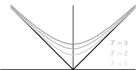
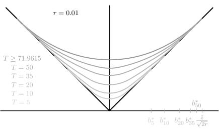
We now consider a Brownian motion and the payoff function . Using the guess-and-verify approach from Remark 4.2 we derive an equilibrium whose structure depends on the discount factor and if also on the size of .
First we focus on . In this case the process , , is a strict submartingale under every . By Remark 5.1 an equilibrium is given by , where and defining via (2.1). The corresponding is given by
For a positive discount factor we first consider the unconstrained optimal stopping problem
where denotes the set of all almost surely finite stopping times. With the usual methods (for more details we refer to [29]) one can show that the optimal stopping time is given by , where ) with and is the unique positive solution of
Note that . Moreover, we have
| (5.1) |
In particular, it holds that
Hence, for all if and only if .
Now we come back to the optimal stopping problem with expectation constraint. If then the optimal stopping time of the unconstrained problem is admissible, i.e. for all . Let
and . The corresponding is given by (5.1). Then all conditions of Theorem 3.7 are satisfied and is an equilibrium strategy.
If then the optimal strategy of the unconstrained optimal stopping problem does not fulfill the expectation constraint for all and, thus, is not admissible.
To find an equilibrium we follow Remark 4.2 and assume that the strategy stops immediately under if is greater than , continues if is sufficiently large, i.e. , but not greater than and stops with rate for small . Here and have to be chosen in such a way that the expectation constraint holds true for all . Observe that (4.3) and (4.4) imply that
| (5.2) | ||||
Using (5.2) it turns out that . Moreover, there exists only one such that the corresponding satisfies the conditions of Theorem 3.7. For this particular the function is continuously differentiable on .
To state the candidate for the equilibrium in more detail let be the unique solution on of
and let
We conclude that
where
Now one can check that is indeed an equilibrium.
Appendix A Appendix
Proof of Lemma 3.3.
Let be non-empty. The Markov property yields
By [22] the functions , (cf. p. 191) and (cf. p. 121) are continuous on . Since as this implies continuity of as claimed. Note that in order to apply [22] one identifies the stopping based on with killing via .
Using estimate 19) from [22, p. 121] as well as their notation, the uniform continuity of the function on yields uniformly. From this the second claim is immediate.
∎
Lemma A.1.
Let be a randomized Markovian time and the function defining via (2.1). Let be some connected component of . Let denote the closure of . If is bounded, then is continuous.
Proof.
Let be a random variable on that is independent of and and let denote the process killed with , i.e.
We extend the function to by setting . Now for the Markov property gives
since for by [22, p. 191] as in the proof of Lemma 3.3 and thus also
The case is analogous.
∎
Lemma A.2.
For every and each function such that and exist (in ), we have
| (A.1) |
Proof.
Without loss of generality we may assume that are bounded and is also bounded away from as well as and , since (A.1) only depends on in a neighborhood of . First we show that in order to prove (A.1) it suffices to verify
| (A.2) | ||||
| and | ||||
| (A.3) | ||||
For this purpose observe
For we choose such that for all and for all . With this we get
An analogous estimate with and replaced by and , respectively, together with shows that (A.2) and (A.3) are in fact sufficient for (A.1).
The transition densities can be estimated as follows:
| (A.4) |
cf. [31, Equation (1.2)]. With this we immediately obtain (A.3) via
Concerning (A.2) we only show as for the other term the argument is exactly the same. Exactly along the lines of the proof of [14, Lemma 5.6] but with the infinitesimal operator in place of the weak infinitesimal operator , as they are called in [14] one can show that
| (A.5) |
if the limit on the right-hand side exists. The argument from Lemma 5.6 of [14] is then applied with the 2-dimensional process on that starts in under as the right continuous Markov process together with the function , . The lemma requires
to be continuous, which is clear due to
Also condition from Lemma 5.6 is met due to Lemma 5.5 in [14].
Applying Fubini’s Theorem we get
Invoking (A.5) our final step in order to prove (A.2) is to show for .
For this purpose we introduce an auxiliary process , defined by . This means . Moreover, we have
and thus
| (A.6) |
For the first inequality is used, which easily follows from (A.4) and the fact that . The second inequality follows form the fact that and cannot hold at once and each implies .
In order to show that the right-hand side of (A.6) goes to 0 for we start with the following estimates. First for using Cauchy-Schwarz inequality and the Itô isometry we get
| (A.7) |
With Fubini’s Theorem, (A.7) and once again the same general technique for we obtain
| (A.8) |
where denotes the Lipschitz constant of . Equation (A.4) and the substitution yield
| (A.9) |
Now let us assume for . Then there exists and a sequence such that for and
for all . By (A.9) there is some such that
for all . This however implies
| (A.10) |
for all . But for sufficiently large , so (A.10) contradicts (A.8). This proves for . Invoking (A.6) the claim follows. ∎
References
- [1] S. Ankirchner, N. Kazi-Tani, M. Klein, and T. Kruse. Stopping with expectation constraints: 3 points suffice. Electron. J. Probab., 24:1 – 16, Paper No. 66, 2019.
- [2] S. Ankirchner, M. Klein, and T. Kruse. A Verification Theorem for Optimal Stopping Problems with Expectation Constraints. Appl. Math. Optim., 79(1):145–177, 2019.
- [3] E. Bayraktar, Z. Wang, and Z. Zhou. Equilibria of time-inconsistent stopping for one-dimensional diffusion processes. arXiv preprint arXiv:2201.07659, 2022.
- [4] E. Bayraktar and S. Yao. Optimal stopping with expectation constraints. arXiv preprint arXiv:2011.04886, 2020.
- [5] E. Bayraktar and S. Yao. Stochastic control/stopping problem with expectation constraints. arXiv preprint arXiv:2305.18664, 2023.
- [6] E. Bayraktar, J. Zhang, and Z. Zhou. Time consistent stopping for the mean-standard deviation problem—the discrete time case. SIAM J. Financial Math., 10(3):667–697, 2019.
- [7] T. Björk, M. Khapko, and A. Murgoci. Time-Inconsistent Control Theory with Finance Applications. Springer Finance. Springer International Publishing, 2021.
- [8] A. Bodnariu, S. Christensen, and K. Lindensjö. Local time pushed mixed stopping and smooth fit for time-inconsistent stopping problems. arXiv preprint arXiv:2206.15124, 2022.
- [9] Y.-L. Chow, X. Yu, and C. Zhou. On dynamic programming principle for stochastic control under expectation constraints. J. Optim. Theory Appl., 185(3):803–818, 2020.
- [10] S. Christensen and K. Lindensjö. On finding equilibrium stopping times for time-inconsistent Markovian problems. SIAM J. Control Optim., 56(6):4228–4255, 2018.
- [11] S. Christensen and K. Lindensjö. On time-inconsistent stopping problems and mixed strategy stopping times. Stochastic Process. Appl., 130(5):2886–2917, 2020.
- [12] S. Christensen and K. Lindensjö. Time-inconsistent stopping, myopic adjustment and equilibrium stability: with a mean-variance application. In Stochastic modeling and control, volume 122 of Banach Center Publ., pages 53–76. Polish Acad. Sci. Inst. Math., Warsaw, 2020.
- [13] S. Christensen and K. Lindensjö. Moment-constrained optimal dividends: precommitment and consistent planning. Adv. in Appl. Probab., 54(2):404–432, 2022.
- [14] E. Dynkin. Markov Processes: Volume 1. Grundlehren der mathematischen Wissenschaften. Springer-Verlag, Berlin Göttingen Heidelberg, 1965.
- [15] E. Dynkin. Markov Processes: Volume 2. Grundlehren der mathematischen Wissenschaften. Springer-Verlag, Berlin Göttingen Heidelberg, 1965.
- [16] S. Ebert, W. Wei, and X. Y. Zhou. Weighted discounting – On group diversity, time-inconsistency, and consequences for investment. J. Econom. Theory, 189:105089, 2020.
- [17] I. Ekeland and A. Lazrak. Being serious about non-commitment: subgame perfect equilibrium in continuous time. arXiv preprint arXiv:math/0604264, 2006.
- [18] Y.-J. Huang and A. Nguyen-Huu. Time-consistent stopping under decreasing impatience. Finance Stoch., 22(1):69–95, 2018.
- [19] Y.-J. Huang, A. Nguyen-Huu, and X. Y. Zhou. General stopping behaviors of naïve and noncommitted sophisticated agents, with application to probability distortion. Math. Finance, 30(1):310–340, 2020.
- [20] Y.-J. Huang and Z. Zhou. The optimal equilibrium for time-inconsistent stopping problems – the discrete-time case. SIAM Journal on Control and Optimization, 57(1):590–609, 2019.
- [21] Y.-J. Huang and Z. Zhou. Optimal equilibria for time-inconsistent stopping problems in continuous time. Mathematical Finance, 30(3):1103–1134, 2020.
- [22] K. Itô and H. McKean. Diffusion Processes and their Sample Paths: Reprint of the 1974 Edition. Grundlehren der mathematischen Wissenschaften. Springer Berlin Heidelberg, 1974.
- [23] D. P. Kennedy. On a constrained optimal stopping problem. J. Appl. Probab., 19(3):631–641, 1982.
- [24] C. Makasu. Bounds for a constrained optimal stopping problem. Optim. Lett., 3(4):499–505, 2009.
- [25] C. W. Miller. Non-linear PDE Approach to Time-Inconsistent Optimal Stopping. SIAM J. Control Optim., 55(1):557–573, 2017.
- [26] J. L. Pedersen and G. Peskir. Optimal mean-variance selling strategies. Math. Financ. Econ., 10(2):203–220, 2016.
- [27] G. Peskir. A Change-of-Variable Formula with Local Time on Surfaces, page 70–96. Springer Berlin Heidelberg, Berlin, Heidelberg, 2007.
- [28] G. Peskir. Optimal detection of a hidden target: the median rule. Stochastic Process. Appl., 122(5):2249–2263, 2012.
- [29] G. Peskir and A. Shiryaev. Optimal stopping and free-boundary problems. Lectures in Mathematics ETH Zürich. Birkhäuser Verlag, Basel, 2006.
- [30] L. Rogers and D. Williams. Diffusions, Markov processes, and Martingales. Vol. 2: Itô Calculus. Cambridge Mathematical Library. Cambridge University Press, second edition, 2000.
- [31] S.-J. Sheu. Some estimates of the transition density of a nondegenerate diffusion markov process. Ann. Probability, 19(2):538–561, 1991.
- [32] R. Strotz. Myopia and inconsistency in dynamic utility maximization. Rev. Econom. Stud., 23(3):165–180, 1955.
- [33] Z. Zhou. Almost strong equilibria for time-inconsistent stopping problems under finite horizon in continuous time. preprint, 2023. http://dx.doi.org/10.2139/ssrn.4431616.