Joint Angle and Delay Cramér-Rao Bound Optimization for Integrated Sensing and Communications

Abstract

In this paper, we study a multi-input multi-output (MIMO) beamforming design in an integrated sensing and communication (ISAC) system, in which an ISAC base station (BS) is used to communicate with multiple downlink users and simultaneously the communication signals are reused for sensing multiple targets. Our interested sensing parameters are the angle and delay information of the targets, which can be used to locate these targets. Under this consideration, we first derive the Cramér-Rao bound (CRB) for angle and delay estimation. Then, we optimize the transmit beamforming at the BS to minimize the CRB, subject to communication rate and power constraints. In particular, we obtain the optimal solution in closed-form in the case of single-target and single-user, and in the case of multi-target and multi-user scenario, the sparsity of the optimal solution is proven, leading to a reduction in computational complexity during optimization. The numerical results demonstrate that the optimized beamforming yields excellent positioning performance and effectively reduces the requirement for a large number of antennas at the BS.

I Introduction

Integrated Sensing and Communication (ISAC) technology is considered one of the promising key technologies for 6G, garnering significant attention from both academia and industry [1]. By integrating sensing capabilities into the conventional cellular network, ISAC opens up numerous application possibilities, such as smart factories, drone monitoring, and intelligent transportation systems. These functionalities demand the system to possess the capability of actively locating targets, a task typically achieved using radar in the past.

Hence, it becomes imperative to investigate the positioning performance of ISAC. Compared with sensing-centric waveform design, communication signal-based waveform design can usually better meet the requirements of current high-speed communication, but it needs to maintain robust sensing performance [2], [3]. To precisely and appropriately define the purpose of sensing, [4], [5] introduced the Cramer-Rao bound (CRB) as a metric for sensing performance evaluation. The CRB enables the analysis of estimation performance for the required sensing parameters. However, their estimation approach often focuses on a single angle parameter or response matrix parameter, which fails to capture the intricate relationship between sensing and communication. Notably, a single parameter may inadequately represent the multifaceted impact of complex functions, such as positioning.

Recently, [6] investigated a multi-base station cooperative positioning ISAC system that locates target through angle and delay estimation due to their excellent positioning performance. However, the sensing metric based on these estimations is rarely considered in ISAC systems. Although a few articles [7], [8] explore location-centered sensing metrics, they still focus on radar-communication coexistence systems, relying on existing radar systems. It is worth noting that while [6] accurately describes the positioning performance, it only considers a single antenna transmitter and studies energy allocation. In reality, current base stations (BSs) typically employ multiple antennas, and distributed structures impose high synchronization requirements on the system. Therefore, this paper addresses these challenges by minimizing the CRB for estimated angle and delay under rate and energy constraints, based on a multi-antenna monostatic BS system.

Specifically, we first derive the CRB for both angle and delay estimation, then, an optimization problem with rate and energy constraints and CRB minimization as the goal is formed to explore the optimal beamforming and communication sensing compromise relationship. In the single-target and single-user scenario, we obtain an optimal solution with a guaranteed rank one and derive a closed-form expression for the optimal solution. In the case of multi-target and multi-user, we prove the sparsity of the solution, simplifying computational complexity. Simulations are conducted to demonstrate the accuracy and effectiveness of our analysis.

II System Model

In this paper, we consider that a BS is equipped with uniform linear array (ULA), containing $N_{t}$ transmit antennas and $N_{r}$ receive antennas ($N_{t}\leq N_{r}$). The whole downlink communication block is leveraged for performing the dual tasks of multiple radar targets localization and communication data transmission, as depicted in Fig. 1. Let $\mathcal{K}=\left\{1,\cdots,K\right\}$ denote the set of communication users (CUs), and $\mathcal{Q}=\left\{1,\cdots,Q\right\}$ denote that of sensing targets. The coordinates of the BS and the $q$-th target are denoted as $({x}_{0},{y}_{0})$ and $({x}_{q},{y}_{q})$, respectively, $q\in\mathcal{Q}$.

For multi-user communication, let $s_{k}(t)$ and $\bm{h}_{k}\in\mathbb{C}^{{{N_{t}}}\times 1}$ denote the transmit signal and the channel vector from the BS to CU $k\in\mathcal{K}$, respectively, the former is a random variable with zero mean and unit variance, and the latter is assumed to be quasi-static and estimated perfectly. Then the received signal at CU $k$ is expressed as

$$y_{k}(t)=\bm{h}_{k}^{H}\bm{w}_{k}s_{k}(t)+\!\sum_{l\neq k,l\in\mathcal{K}}\!\bm{h}_{k}^{H}\bm{w}_{l}s_{l}(t)+n_{k}(t),$$ (1)

where $\bm{w}_{k}\in\mathbb{C}^{{{N_{t}}}\times 1}$ is the beamforming vector of the $k$-th CU, $n_{k}(t)\sim\mathcal{CN}(0,\sigma_{k}^{2})$ denotes the noise at the receiver of CU $k$, which means that $n_{k}(t)$ is a circularly symmetric complex Gaussian (CSCG) random variable with zero mean and variance $\sigma_{k}^{2}$. The corresponding achievable rate of $k$-th CU is given by $R=\log_{2}(1+\gamma_{k})$ where ${\rm\gamma}_{k}=\frac{\left|\bm{h}_{k}^{H}\bm{w}_{k}\right|^{2}}{\sum\limits_{l\neq k,l\in\mathcal{K}}\lvert\bm{h}_{k}^{H}\bm{w}_{l}\rvert^{2}+\sigma_{k}^{2}},\forall k\in\mathcal{K}$.

Figure 1: An illustration of the system.

Next, we consider the multi-target sensing, in which the communication signals $s_{k}(t)$’s are reused for sensing. Suppose that the radar processing is implemented over an interval $\mathcal{T}$ with duration $T$, which is sufficiently long so that $\int_{\mathcal{T}}\lvert s_{k}(t)\rvert^{2}dt=T\cdot\mathbb{E}\left[\lvert s_{k}(t)\rvert^{2}\right]=T$ and $\int_{\mathcal{T}}s_{k}(t)s^{*}_{l}(t)dt=T\cdot\mathbb{E}\left[s_{k}(t)s^{*}_{l}(t)\right]=0$, $\forall k\neq l$. Then the reflected echoes received at the BS can be given in the form

$$\bm{r}(t)=\sum_{q=1}^{Q}\sum_{k=1}^{K}\alpha_{q}\bm{a}(\theta_{q})\bm{b}(\theta_{q})^{T}\bm{w}_{k}s_{k}(t-\tau_{q})+\bm{n}_{r}(t),$$ (2)

where $\bm{n}_{r}(t)\sim\mathcal{CN}(\bm{0},\bm{R})$ denotes the complex additive white Gaussian noise, $\alpha_{q}$ is a complex amplitude capturing the effects of the target radar cross section (RCS) and the path loss for the radar propagation path between the BS and target $q$. $\theta_{q}$ is the azimuth angle of the $q$-th target relative to the BS, $\bm{b}(\theta_{q})\in\mathbb{C}^{{{N_{t}}}\times 1}$ and $\bm{a}(\theta_{q})\in\mathbb{C}^{{{N_{r}}}\times 1}$ are transmit and receive steering vectors of the antenna array of the BS. Here, we choose the center of the ULA antennas as the reference point, which means the transmit steering vector and its derivative are expressed as ${\mathbf{b}}\left(\theta\right)={\left[{{e^{-j\frac{{{N_{t}-1}}}{2}\pi\sin\theta}},{e^{-j\frac{{{N_{t}}-3}}{2}\pi\sin\theta}},\ldots,{e^{j\frac{{{N_{t}-1}}}{2}\pi\sin\theta}}}\right]^{T}}$, ${\mathbf{\dot{b}}}\left(\theta\right)={\left[{-j{b_{1}}\frac{{{N_{t}-1}}}{2}\pi\cos\theta,\ldots,j{b_{{N_{t}}}}\frac{{{N_{t}-1}}}{2}\pi\cos\theta}\right]^{T}}$, where $b_{i}$ represents the $i$-th entry of ${\mathbf{b}}\left(\theta\right)$. The receive steering vector and its derivative have similar form. According to the symmetry, it can be easily verified that ${{\mathbf{b}}^{H}}{\mathbf{\dot{b}}}=0,{{\mathbf{a}}^{H}}{\mathbf{\dot{a}}}=0,\forall\theta$, where ${{\mathbf{b}}}$, ${{\mathbf{a}}}$, ${{\mathbf{\dot{b}}}}$, and ${{\mathbf{\dot{a}}}}$ denote ${{\mathbf{b}}}\left(\theta\right)$, ${{\mathbf{a}}}\left(\theta\right)$, ${{\mathbf{\dot{b}}}}\left(\theta\right)$, and ${{\mathbf{\dot{a}}}}\left(\theta\right)$, respectively. $\tau_{q}$ denotes the propagation delay associated with $k$-th signal and $q$-th target, and can be expressed as $\tau_{q}=\frac{\sqrt{({x}_{q}-{x}_{0})^{2}\!+({y}_{q}-{y}_{0})^{2}}}{2c}\triangleq\frac{R_{q}}{2c}$, where $c$ is the speed of electromagnetic wave.

III Estimation CRB Derivation

This section provides the derivation results for the CRB of angle and delay in the general case. Denote the $2Q\times 1$ vector of unknown target parameters as $\bm{\varsigma}\triangleq\left[\bm{\theta}^{T},\bm{\tau}^{T}\right]^{T}$, with $\bm{\theta}\triangleq\left[\theta_{1},\ldots,\theta_{Q}\right]^{T}$ and $\bm{\tau}\triangleq\left[\tau_{1},\ldots,\tau_{Q}\right]^{T}$. For an unbiased estimator $\bm{\varsigma}$, the covariance matrix is lower bounded as $\bm{C}_{\hat{\bm{\varsigma}}}=\mathbb{E}\left\{(\hat{\bm{\varsigma}}-\bm{\varsigma})(\hat{\bm{\varsigma}}-\bm{\varsigma})^{H}\right\}\geq\bm{C}_{\mathrm{CRB}}$. Based on the received echo signal at the BS, we can obtain the Fisher information matrix (FIM) for the parameters estimation as shown in the following theorem.

Theorem 1

The FIM $\bm{F}$ for estimating $\bm{\varsigma}$ is given by

$$\bm{F}=\left[\begin{array}[]{ll}\bm{F}_{\bm{\theta},\bm{\theta}}&\bm{F}_{\bm{\theta},\bm{\tau}}\\ \bm{F}_{\bm{\tau},\bm{\theta}}&\bm{F}_{\bm{\tau},\bm{\tau}}\end{array}\right]=\frac{2}{\sigma^{2}}\operatorname{Re}\left[\begin{array}[]{ll}\bm{F}_{\bm{\theta},\bm{\theta}}^{\prime}&\bm{F}_{\bm{\theta},\tau}^{\prime}\\ \bm{F}_{\bm{\tau},\bm{\theta}}^{\prime}&\bm{F}_{\bm{\tau},\bm{\tau}}^{\prime}\end{array}\right],$$ (3)

where

$$\bm{F}^{\prime}_{\bm{\theta},\bm{\theta}} =\left(\left(\dot{\bm{A}}^{H}\dot{\bm{A}}\right)\odot\left(\bm{C}^{*}\bm{B}^{H}\left(\bm{W}\bm{s}\bm{s}^{H}\bm{W}^{H}\right)^{*}\bm{B}\bm{C}\right)\right.$$ (4)

$$\left.+\left(\dot{\bm{A}}^{H}\bm{A}\right)\odot\left(\bm{C}^{*}\bm{B}^{H}\left(\bm{W}\bm{ss}^{H}\bm{W}^{H}\right)^{*}\dot{\bm{B}}\bm{C}\right)\right.$$

$$\left.+\left(\bm{A}^{H}\dot{\bm{A}}\right)\odot\left(\bm{C}^{*}\dot{\bm{B}}^{H}\left(\bm{W}\bm{s}\bm{s}^{H}\bm{W}^{H}\right)^{*}\bm{BC}\right)\right.$$

$$\left.+\left(\bm{A}^{H}\bm{A}\right)\odot\left(\bm{C}^{*}\dot{\bm{B}}^{H}\left(\bm{W}\bm{s}\bm{s}^{H}\bm{W}^{H}\right)^{*}\dot{\bm{B}}\bm{C}\right)\right),$$

$$\bm{F}^{\prime}_{\bm{\theta},\bm{\tau}} =\bm{F}^{\prime T}_{\bm{\tau},\bm{\theta}}$$ (5)

$$=\left(\left(\dot{\bm{A}}^{H}\bm{A}\right)\odot\left(\bm{C}^{\bm{*}}\bm{B}^{H}\left(\bm{Wss}^{H}\bm{W}^{H}\right)^{\bm{*}}\bm{BC}(-j\omega)\right)\right.$$

$$\left.+\left(\bm{A}^{H}\bm{A}\right)\odot\left(\bm{C}^{*}\bm{B}^{H}\left(\bm{W}\bm{s}\bm{s}^{H}\bm{W}^{H}\right)^{*}\bm{BC}\right)(-j\omega)\right),$$

$$\bm{F}^{\prime}_{\bm{\tau},\bm{\tau}}=\left(\left(\bm{A}^{H}\bm{A}\right)\odot\left(\bm{C}^{\bm{*}}\bm{B}^{H}\left(\bm{W}\bm{s}\bm{s}^{H}\bm{W}^{H}\right)^{*}\bm{B}\bm{C}\right)\right).$$ (6)

Proof:

See Appendix A. ∎

As a result, $\bm{C}_{\mathrm{CRB}}({\bm{w}_{k}})=\bm{F}^{-1}$, which is used as the sensing performance metric in the following.

IV Transmit Beamforming Design

In this section, we form the optimization problem based on CRB and communication rate as the performance index. Because we are estimating a vector of parameters, the CRB is a matrix. To obtain a scalar objective function, [11] introduced several CRB-based scalar metrics for optimization. In this paper, we choose the objective function $\operatorname{Tr}(\bm{C}_{\rm{CRB}})$ based on tracing that can balance the units used for different target parameters via an average sense, leading to the following optimization problem

$$\min_{\bm{w}_{k}}\quad \operatorname{Tr}(\bm{C}_{\rm{CRB}})$$ (7a)

s.t. $$\log_{2}\left(1+\gamma_{k}\right)\geq\Gamma_{k},\forall k\in\mathcal{K}\text{, }$$ (7b)

$$\sum\nolimits_{k=1}^{K}\|\bm{w}_{k}\|^{2}\leq P_{T}\text{,}$$ (7c)

where $\Gamma_{k}$ denotes the rate threshold of $k$-th CU, $P_{T}$ is the transmit power budget, and $\|\cdot\|$ denotes the Euclidean norm. Next, we analyze the problem in two cases, and give some insights about the solution to the problem.

IV-A Single-Target and Single-User Case

For CU 1 and the target, let $\sigma_{c}^{2}$, $\alpha$ be the noise power and complex amplitude. Since both $\bm{F}_{\bm{\theta},\bm{\theta}}$ and $\bm{F}_{\bm{\tau},\bm{\tau}}$ are scalars and $F_{\theta,\tau}=F_{\tau,\theta}=0$ in this scenario, the minimization of $\operatorname{Tr}(\bm{C}_{\rm{CRB}})$ can be converted to the maximization of $F_{\theta,\theta}+F_{\tau,\tau}$, which can be calculated from Theorem 1 with the orthogonality property, and the values of $F_{\theta,\theta}$ and $F_{\tau,\tau}$ are $\frac{2|\alpha|^{2}}{\sigma^{2}}\big{(}\|\dot{\bm{a}}\|^{2}|\bm{b}^{H}\bm{w}_{1}|^{2}+\|\bm{a}\|^{2}|\dot{\bm{b}}^{H}\bm{w}_{1}|^{2}\big{)}$ and $\frac{2\omega^{2}|\alpha|^{2}}{\sigma^{2}}(\|\bm{a}\|^{2}|\bm{b}^{H}\bm{w}_{1}|^{2})$. Then, the original question becomes

$$\max_{\bm{w}_{1}}\quad \frac{2|\alpha|^{2}}{\sigma^{2}}\left(\|\dot{\bm{a}}\|^{2}\left|\bm{b}^{H}\bm{w}_{1}\right|^{2}\!+\!\|\bm{a}\|^{2}\left|\dot{\bm{b}}^{H}\bm{w}_{1}\right|^{2}\!\right.$$

$$\left.+\omega^{2}\|\bm{a}\|^{2}\left|\bm{b}^{H}\bm{w}_{1}\right|^{2}\right)$$ (8a)

s.t. $$\left|\bm{h}_{1}^{H}\bm{w}_{1}\right|^{2}\geq\left(2^{\Gamma_{1}}-1\right)\sigma_{c}^{2}\text{, }$$ (8b)

$$\|\bm{w}_{1}\|^{2}\leq P_{T},$$ (8c)

which is a non-convex quadratically constrained quadratic programming (QCQP), and we can solve it via semidefinite relaxation(SDR) with $\bm{W}_{1}=\bm{w}_{1}\bm{w}_{1}^{H}$. So (8) can turn into

$$\max_{\bm{W}_{1}}\quad \operatorname{Tr}\left(\hat{\bm{G}}\bm{W}_{1}\right)$$ (9a)

s.t. $$\operatorname{Tr}\left(\hat{\bm{H}}\bm{W}_{1}\right)\geq\left(2^{\Gamma_{1}}-1\right)\sigma_{c}^{2}\text{, }$$ (9b)

$$\operatorname{Tr}\left(\bm{W}_{1}\right)\leq P_{T}\text{. }$$ (9c)

where $\hat{\bm{G}}=\frac{2|\alpha|^{2}}{\sigma^{2}}\left(\|\dot{\bm{a}}\|^{2}\bm{b}\bm{b}^{H}+\|\bm{a}\|^{2}\dot{\bm{b}}\dot{\bm{b}}^{H}+\omega^{2}\|\bm{a}\|^{2}\bm{b}\bm{b}^{H}\right)$ and $\hat{\bm{H}}=\bm{h}_{1}\bm{h}_{1}^{H}$. Although the rank-1 constraint is removed for the convexity of the problem, the optimal solution has been proved rigorously to have the rank-1 property in [12]. Further, we give a closed-form solution to problem (8) in the following theory.

Theorem 2

When $\left|\bm{h}_{1}^{H}\bm{w}_{1}\right|^{2}\geq\left(2^{\Gamma_{1}}-1\right)\sigma_{c}^{2}$, the optimal solution to problem (8) is

$$\bm{w}_{1}=\left\{\begin{array}[]{l}{x_{1}\bm{d}_{x}+x_{3}\bm{d}_{z},\|\dot{\bm{a}}\|^{2}+\omega^{2}\|\bm{a}\|^{2}>\|\bm{a}\|},\\ {c_{0}\bm{d}_{x}+x_{2}\bm{d}_{y}+x_{3}\bm{d}_{z},\|\dot{\bm{a}}\|^{2}+\omega^{2}\|\bm{a}\|^{2}\leq\|\bm{a}\|,}\\ \end{array}\right.$$ (10)

where $\bm{d}_{z}=\bm{h}_{1}-\frac{\bm{h}_{1}-\bm{d}_{x}^{H}\bm{h}_{1}\bm{d}_{x}}{\left\|\bm{h}_{1}-\bm{d}_{x}^{H}\bm{h}_{1}\bm{d}_{x}\right\|}-\frac{\bm{h}_{1}-\bm{d}_{y}^{H}\bm{h}_{1}\bm{d}_{y}}{\left\|\bm{h}_{1}-\bm{d}_{y}^{H}\bm{h}_{1}\bm{d}_{y}\right\|},\\ \bm{d}_{x}=\frac{\bm{b}}{\|\bm{b}\|},\bm{d}_{y}=\frac{\dot{\bm{b}}}{\|\dot{\bm{b}}\|}$, $x_{1}=\sqrt{P_{T}-x_{3}^{2}}=\sqrt{P_{T}-\frac{\left(2^{\Gamma_{1}}-1\right)\sigma_{c}^{2}}{\|\bm{h}_{1}\|^{2}}},\\ x_{2}=\sqrt{P_{T}-\frac{\left(2^{\Gamma_{1}}-1\right)\sigma_{c}^{2}}{\|\bm{h}_{1}\|^{2}}-c_{0}^{2}},x_{3}=\sqrt{\frac{\left(2^{\Gamma_{1}}-1\right)\sigma_{c}^{2}}{\|\bm{h}_{1}\|^{2}}}$, and $c_{0}$ is a threshold defined in Appendix B. Otherwise, the optimal solution is the same as (10) with $x_{3}=0$.

Proof:

See Appendix B. ∎

IV-B Multi-Target and Multi-User Case

We first analyze the relationship between the elements of the FIM and $\bm{w}_{k}$. Based on $\bm{r}_{1}=\bm{ACB}{}^{T}\bm{W}\bm{s}+\bm{n}_{1}$, which is defined in Appendix A, we let $\bm{D}=\bm{ACB}{}^{T}$, and assume that $\dot{\bm{D}}_{m}$ is the derivative with respect to $\bm{\varsigma}_{m}$, then

$$[\bm{F}]_{mn} =2\operatorname{Re}\operatorname{Tr}\left(\frac{\partial\bm{\mu}^{H}}{\partial\bm{\varsigma}_{m}}\bm{R}^{-1}\frac{\partial\bm{\mu}}{\partial\bm{\varsigma}_{n}}\right)$$ (11)

$$=\frac{2}{\sigma^{2}}\operatorname{Re}\left\{\bm{w}_{v}^{H}\left(\left(\bm{s}^{*}\bm{s}^{T}\right)\otimes\dot{\bm{D}}_{m}^{H}\dot{\bm{D}}_{n}\right)\bm{w}_{v}\right\},$$

where $\bm{w}_{v}=\operatorname{vec}(\bm{W})$ and $\otimes$ represents the Kronecker product, while the optimization problem is

$$\min_{\bm{w}_{v}}\quad \operatorname{Tr}(\bm{C}_{\rm{CRB}})$$ (12a)

s.t. $$\frac{\left|\bm{g}_{k}^{H}\bm{w}_{v}\right|^{2}}{\bm{w}_{v}^{H}\bm{L}_{k}\bm{w}_{v}+\sigma_{k}^{2}}\geq\left(2^{\Gamma_{k}}-1\right),\forall k\in\mathcal{K},$$ (12b)

$$\|\bm{w}_{v}\|^{2}\leq P_{T},$$ (12c)

where $\bm{g}_{k}=\bm{e}_{k}\otimes\bm{h}_{k}$, $\bm{L}_{k}=\left(\bm{1}-\bm{e}_{k}\right)\left(\bm{1}-\bm{e}_{k}\right)^{T}\otimes\bm{h}_{k}\bm{h}_{k}^{H}$, and $\bm{e}_{k}=[\underbrace{0,\ldots,0}_{k-1},1,\underbrace{0,\ldots,0}_{N_{t}-k}]^{T}$, $\bm{1}$ represents a vector in which all elements are 1. (12) yields that the target function and rate constraints are non-convex with respect to $\bm{w}_{v}$. Upon letting $\bm{W}_{v}=\bm{w}_{v}\bm{w}_{v}^{H}$, (12) can be relaxed to (by removing the constraint $\operatorname{rank}(\bm{W}_{v})=1)$)

$$\min_{\bm{W}_{v},\left\{t_{q}\right\}_{q=1}^{2Q}} \bm{1}^{T}\bm{t}$$ (13a)

s.t. $$\left[\begin{array}[]{ll}\bm{F}&\bm{e}_{k}\\ \bm{e}_{k}^{T}&t_{q}\end{array}\right]\succeq 0\text{,}\forall k\in\mathcal{K},$$ (13d)

$$\frac{\operatorname{Tr}\left(\bm{g}_{k}\bm{g}_{k}^{H}\bm{W}_{v}\right)}{\operatorname{Tr}\left(\bm{L}_{k}\bm{W}_{v}\right)+\sigma_{k}^{2}}\geq\left(2^{\Gamma_{k}}-1\right),\forall k\in\mathcal{K},$$ (13e)

$$\operatorname{Tr}\left(\bm{W}_{v}\right)\leq P_{T},$$ (13f)

where $\bm{t}$ is a newly introduced auxiliary variable and its elements are $\left\{t_{q}\right\}_{q=1}^{2Q}$. It can be observed from (11) and Appendix A that $\bm{F}$ is a linear function of $\bm{W}_{v}$, which implies that (13) is a convex semidefinite program (SDP) and thus can be handled via standard convex optimization tools [13]. Further, the following proposition gives the covariance matrix for the solution of problem (13).

Proposition 1

The beamforming covariance matrix $\bm{W}^{*}_{v}$ obtained as the solution to (13) can be expressed as

$$\bm{W}_{v}^{*}=\bm{U}_{T}\bm{\Lambda}\bm{U}_{T}^{H},$$ (14)

where $\bm{U}_{T}\triangleq[\bm{B},\dot{\bm{B}}]^{*}$, and $\bm{\Lambda}\in\mathbb{C}^{2Q\times 2Q}$ is a positive semidefinite matrix.

Proof:

See Appendix C. ∎

The highlight of Proposition 1 is that it can significantly reduce the computational burden of solving (13), because the optimization can equivalently be performed over $\bm{\Lambda}$ instead of $\bm{W}_{v}$ and usually $N_{r}\gg Q$.

V NUMERICAL RESULTS

In this section, the numerical results are provided to clarify the previous analysis and the validity of beamforming. We set the BS equipped with $N_{t}=16$ and $N_{r}=20$ antennas, serving $K=3$ CUs and locating $Q=3$ radar targets. The interval between adjacent antennas of the BS is half-wavelength. The angles of the CUs and targets are set in the range $[-\frac{\pi}{2},\frac{\pi}{2}]$. The overall power budget is $P_{T}=20$ dBm and the noise variances are set as $\sigma_{k}^{2}=-90$ dBm, $\sigma^{2}=-10$ dBm. For single-target and single-user case, the line of sight (LoS) model is considered for the channel from the BS to the CU with the path loss -70 dB. For multi-target and multi-user case, the communication channel is set as Rayleigh fading like [7].

Figure 2: The transmit beampattern for single-target and single-user case, where the target and CU are located respectively at spatial angles $0^{\circ}$ and $40^{\circ}$.

Fig. 2 shows the resultant beampatterns where $\Gamma_{1}=7.5$ bps/Hz, it can be observed that the sensing performance of the closed-form solution satisfying SINR constraint is similar to that of the optimized solution, and the communication performance is improved. This is because the closed-form solution has a margin on the boundary of the SINR constraint, and the corresponding sensing performance is slightly decreased. When the SINR constraint cannot be satisfied, the energy is no longer allocated to the CU, and the best sensing performance can be obtained. Compared with the scheme that uses the term “only $\theta$” to represent the beamforming in [7], the optimal solution obtained through the method in this paper almost coincides with it in Fig. 2, which indicates that the proposed method in this paper takes into account the angle estimation performance while ensuring the delay estimation performance.

(a) CRB of $\theta$ versus $P_{T}$.

(b) CRB of $\tau$ versus $P_{T}$.

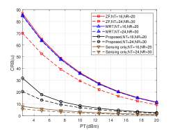
(c) CRB of positioning versus $P_{T}$.

Figure 3: The CRB of estimated parameters versus $P_{T}$.

Fig. 3 show the relationship between CRB of the estimated parameters and total transmitted energy, where “CRB(u)” represents the lower bound on the estimate of the Cartesian coordinates of the targets, and its definition is as follows: $\rm{CRB}(u)=[\operatorname{Tr}(\widetilde{\bm{J}}^{-1})]^{1/2}$. $\widetilde{\rm\bm{J}}=(\frac{\partial\bm{\varsigma}}{\partial\bm{u}})\bm{F}(\frac{\partial\bm{\varsigma}}{\partial\bm{u}})^{T}$ is derived by the chain rule, and $\bm{u}$ is a vector containing the coordinates of all the targets. From Fig. 3(a) and Fig. 3(b), it can be seen that the parameter estimation performance of the beamforming scheme proposed in this paper is significantly better than that of the two linear beamforming schemes [15], zero-forcing (ZF) and maximum-ratio transmission (MRT), and is close to the ideal situation “sensing only” which is obtained without the rate constraints. When the number of antennas increases, the angle estimation performance can be better improved, since this improves the resolution of array to the angle, while the delay and positioning estimation performance in Fig. 3(c) are little improved, which shows the necessity of joint parameters estimation. Synthesize the above analysis, the proposed beamforming scheme can effectively reduce the dependence of the BS on the number of antennas and achieve excellent position estimation performance with low power consumption.

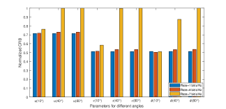
Figure 4: Normalized CRB of parameters at different angles, where the targets are at $\Theta_{r}=\left\{-30^{\circ},0^{\circ},15^{\circ}\right\}$, and the CUs are at $\Theta_{c}=\left\{10^{\circ},40^{\circ},80^{\circ}\right\}$.

Fig. 4 shows the impact of CUs at different locations on the compromise between sensing and communication performance. It can be seen that as the angle increases (meaning the distance between CU and targets increases), the same communication rate will cause more serious loss of estimation performance. It is worth noting that increasing the communication requirement in the 10° direction will improve the angle estimation performance, because the CU and the sensing target overlap in the beam energy domain, but the positioning estimation performance of the targets is still decreased, since the delay estimation performance is not improved.

VI Conclusion

This paper focused on the beamforming optimization problem that aims to maximize the sensing performance while adhering to rate and energy constraints. Through analysis of special and generalized scenarios, we obtained the closed-form solution and prove the sparsity of the optimal solution, effectively reducing operational complexity. We also observed that a single parameter is insufficient to describe the positioning function adequately, prompting further investigation into the impact of CU distribution on positioning performance, which presents an intriguing avenue for future research.

Appendix A Proof of Theorem 1

Taking the discrete Fourier transform (DFT) for the reflected data received at the BS, the frequency-domain expression of (2) can be obtained in the form [9]

$${\bm{r}}_{1}(\omega)=\sum_{q=1}^{Q}\sum_{k=1}^{K}\alpha_{q}{\bm{a}}(\theta_{q})b(\theta_{q})^{T}{\bm{w}}_{k}e^{-j\omega\tau_{q}}s_{k}(\omega)+{\bm{n}}_{1}(\omega),$$ (15)

where $s_{k}(\omega)$ represents the DFT of $s_{k}(t)$, ${\bm{n}}_{1}(\omega)\sim\mathcal{CN}(\bm{0},\bm{R})$ is the form of noise in frequency domain, and $\bm{R}=\sigma^{2}\bm{I}_{N_{r}}$, $\bm{I}$ represents the identity matrix. Considering the actual signal pulse shaping and calculation simplification, we set $s_{k}(\omega)=1$. To simply notation, we denote $\bm{A}=\left[\bm{a}\left(\theta_{1}\right),\ldots,\bm{a}\left(\theta_{Q}\right)\right]$, $\bm{B}=\left[\bm{b}\left(\theta_{1}\right),\ldots,\bm{b}\left(\theta_{Q}\right)\right]$, $\bm{C}=\operatorname{diag}(\bm{c})$, $\bm{c}=\left[\alpha_{1}e^{-j\omega\tau_{1}},\ldots,\alpha_{Q}e^{-j\omega\tau_{Q}}\right]^{T}$, $\bm{W}=\left[\bm{w}_{1},\ldots,\bm{w}_{K}\right]$, $\bm{s}=[1,\ldots,1]^{T},\bm{s}\in\mathbb{C}^{K\times 1}$, then, (15) can be rewritten as $\bm{r}_{1}=\bm{ACB}{}^{T}\bm{W}\bm{s}+\bm{n}_{1}$. Using the Slepian-Bangs formula [10], for the complex observation vector $\bm{r}_{1}\sim\mathcal{CN}(\bm{\mu},\bm{R})$, in which $\bm{\mu}=\bm{ACB}{}^{T}\bm{W}\bm{s}$, the $(m,n)$-th element of FIM $\bm{F}$ is

$${[\bm{F}]_{mn}\!=\!\operatorname{Tr}\left(\bm{R}^{-1}\frac{\partial\bm{R}}{\partial\bm{\varsigma}_{m}}\bm{R}^{-1}\frac{\partial\bm{R}}{\partial\bm{\varsigma}_{n}}\right)\!+\!2\operatorname{Re}\operatorname{Tr}\left(\frac{\partial\bm{\mu}^{H}}{\partial\bm{\varsigma}_{m}}\bm{R}^{-1}\frac{\partial\bm{\mu}}{\partial\bm{\varsigma}_{n}}\right).}$$ (16)

Since the covariance matrix $\bm{R}$ does not depend on the parameters to be estimated, we only have to worry about the second term in (16). Let $\dot{\bm{B}}\triangleq[\frac{\partial\bm{b}(\theta_{1})}{\partial\theta_{1}},\ldots,\frac{\partial\bm{b}(\theta_{Q})}{\partial\theta_{Q}}]$ and $\dot{\bm{A}}\triangleq[\frac{\partial\bm{a}(\theta_{1})}{\partial\theta_{1}},\ldots,\frac{\partial\bm{a}(\theta_{Q})}{\partial\theta_{Q}}]$, it follows that $\frac{\partial\bm{\mu}}{\partial{\theta}_{q}}=\dot{\bm{A}}\bm{e}_{q}\bm{e}_{q}^{T}\bm{C}\bm{B}^{T}\bm{W}\bm{s}+\bm{A}\bm{C}\bm{e}_{q}\bm{e}_{q}^{T}\dot{\bm{B}}^{T}\bm{W}\bm{s}$, $\frac{\partial\bm{\mu}}{\partial\tau_{q}}=(-j\omega)\bm{A}\bm{C}\bm{e}_{q}\bm{e}_{q}^{T}\bm{B}^{T}\bm{W}\bm{s},$ where $\bm{e}_{q}$ denotes the $q$-th column of $\bm{I}_{Q}$. Taking the submatrix $\bm{F}_{\bm{\theta},\bm{\theta}}$ for example, then

$$\left[\bm{F}_{\bm{\theta},\bm{\theta}}\right]_{pq}= 2\mathrm{Re}\mathrm{Tr}\big{(}\dot{\bm{A}}\bm{e}_{p}\bm{e}_{p}^{T}\bm{C}\bm{B}^{T}\bm{W}\bm{s}+\bm{A}\bm{C}\bm{e}_{p}\bm{e}_{p}^{T}\dot{\bm{B}}^{T}\bm{W}\bm{s})^{H}$$ (17)

$$\times\bm{R}^{-1}(\dot{\bm{A}}\bm{e}_{q}\bm{e}_{q}^{T}\bm{CB}^{T}\bm{W}\bm{s}+\bm{A}\bm{C}\bm{e}_{q}\bm{e}_{q}^{T}\dot{\bm{B}}^{T}\bm{W}\bm{s})\bigr{)},$$

next take one of the four product terms in (17), note that

$$\operatorname{Tr} \left(\left(\dot{\bm{A}}\bm{e}_{p}\bm{e}_{p}^{T}\bm{C}\bm{B}^{T}\bm{W}\bm{s}\right)^{H}\bm{R}^{-1}\left(\dot{\bm{A}}\bm{e}_{q}\bm{e}_{q}^{T}\bm{C}\bm{B}^{T}\bm{W}\bm{s}\right)\right)$$ (18)

$$=\bm{e}_{p}^{T}\left(\dot{\bm{A}}^{H}\bm{R}^{-1}\dot{\bm{A}}\right)\bm{e}_{q}\bm{e}_{q}^{T}\left(\bm{C}\bm{B}^{T}\bm{W}\bm{ss}^{H}\bm{W}^{H}\bm{B}^{*}\bm{C}^{H}\right)\bm{e}_{p}$$

$$=\left(\dot{\bm{A}}^{H}\bm{R}^{-1}\dot{\bm{A}}\right)_{pq}\left(\bm{C}^{*}\bm{B}^{H}\left(\bm{W}\bm{s}\bm{s}^{H}\bm{W}^{H}\right)^{*}\bm{B}\bm{C}\right)_{pq},$$

where $\bm{X}_{pq}$ denotes $(p,q)$-th element of $\bm{X}$. The other three matrix product terms in (17) have similar forms. And $\bm{R}=\sigma^{2}\bm{I}_{N_{r}}$, hence, $\bm{F}_{\bm{\theta},\bm{\theta}}=\frac{2}{\sigma^{2}}\operatorname{Re}(\bm{F}^{\prime}_{\bm{\theta},\bm{\theta}})$, with $\bm{F}^{\prime}_{\bm{\theta},\bm{\theta}}$ given in (4). Similar to the steps above, we can obtain the results given in (5) and (6), respectively, in which $\odot$ represents the Hadamard (element-wise) product. As a result, the Theorem 1 is proved.

Appendix B Proof of Theorem 2

First of all, the optimal solution of (8) satisfies $\bm{w}_{1}\in\operatorname{span}\{\bm{b},\dot{\bm{b}},\bm{h}_{1}\}$, which has been proved in [7], and the basic idea is to project the beamforming onto direction directly related to the target function and constraint. It’s not hard to imagine that the optimum is reached when the power budget is fully utilized. Hence, the optimal $\bm{w}_{1}$ can be expressed as

$$\bm{w}_{1}=x_{1}\bm{d}_{x}+x_{2}\bm{d}_{y}+x_{3}\bm{d}_{z},x_{1},x_{2},x_{3}\in\mathbb{C},$$ (19)

for $\operatorname{span}\{\bm{d}_{x},\bm{d}_{y},\bm{d}_{z}\}=\operatorname{span}\{\bm{b},\dot{\bm{b}},\bm{h}_{1}\}$. When the SINR constraint is active, problem (8) can be rewritten as

$$\max_{\bm{w}_{1}}\quad \frac{2|\alpha|^{2}}{\sigma^{2}}\left(\left(\|\dot{\bm{a}}\|^{2}+\omega^{2}\|\bm{a}\|^{2}\right)x_{1}^{2}+\|\bm{a}\|^{2}x_{2}^{2}\right)$$ (20a)

s.t. $$x_{3}^{2}\|\bm{h}_{1}\|^{2}=\left(2^{\Gamma_{1}}-1\right)\sigma_{c}^{2}\text{, }$$ (20b)

$$x_{1}^{2}+x_{2}^{2}=P_{T}-x_{3}^{2}\text{, }$$ (20c)

which yields that $x_{3}=\sqrt{\frac{\left(2^{\Gamma_{1}}-1\right)\sigma_{c}^{2}}{\|\bm{h}_{1}\|^{2}}}$. Maximizing the objective function now depends on the relative sizes of $\|\dot{\bm{a}}\|^{2}+\omega^{2}\|\bm{a}\|^{2}$ and $\|\bm{a}\|^{2}x_{2}^{2}$, it’s intuitive that the target function maximizes when $x_{1}=0$ or $x_{2}=0$. Interestingly, however, in the case of single-target and single-user, $F_{\theta,\theta}=\frac{2|\alpha|^{2}}{\sigma^{2}}\big{(}\|\dot{\bm{a}}\|^{2}|\bm{b}^{H}\bm{w}_{1}|^{2}+\|\bm{a}\|^{2}|\dot{\bm{b}}^{H}\bm{w}_{1}|^{2}\big{)}$ and $F_{\tau,\tau}=\frac{2\omega^{2}|\alpha|^{2}}{\sigma^{2}}(\|\bm{a}\|^{2}|\bm{b}^{H}\bm{w}_{1}|^{2})$, if $x_{1}=0$, the estimated performance for $\tau$ is probably going to be very bad, which is hard to accept in practice. So we give $x_{1}$ a minimum threshold $c_{0}$ that we can tolerate. Then, if $\|\dot{\bm{a}}\|^{2}+\omega^{2}\|\bm{a}\|^{2}>\|\bm{a}\|$, it follows that $x_{2}=0,x_{1}=\sqrt{P_{T}-x_{3}^{2}}=\sqrt{P_{T}-\frac{\left(2^{\Gamma_{1}}-1\right)\sigma_{c}^{2}}{\|\bm{h}_{1}\|^{2}}}$, otherwise, we have $x_{1}=c_{0}$ and $x_{2}=\sqrt{P_{T}-\frac{\left(2^{\Gamma_{1}}-1\right)\sigma_{c}^{2}}{\|\bm{h}_{1}\|^{2}}-c_{0}^{2}}$, $x_{3}=\sqrt{\frac{\left(2^{\Gamma_{1}}-1\right)\sigma_{c}^{2}}{\|\bm{h}_{1}\|^{2}}}$. When the SINR constraint is inactive, we should fully allocate the power along the direction of $\bm{b}$ and $\dot{\bm{b}}$, which means that $x_{3}=0$. Problem (8) changes to

$$\max_{\bm{w}_{1}}\quad \frac{2|\alpha|^{2}}{\sigma^{2}}\left(\left(\|\dot{\bm{a}}\|^{2}+\omega^{2}\|\bm{a}\|^{2}\right)x_{1}^{2}+\|\bm{a}\|^{2}x_{2}^{2}\right)$$ (21a)

s.t. $$x_{1}^{2}+x_{2}^{2}=P_{T}\text{,}$$ (21b)

which can be analysized in the same way as the previous argument. This results in the expressions in Theorem 2, which completes the proof.

Appendix C Proof of Proposition 1

We know that FIM and $\bm{W}_{v}$ are connected by $\bm{B}$ and $\dot{\bm{B}}$ on account of Theorem 1. Decompose $\bm{W}_{v}^{*}=\bm{\Omega}_{U_{T}}\bm{W}_{v}^{*}+\bm{\Omega}_{U_{T}}^{\perp}\bm{W}_{v}^{*}$, in which $\bm{\Omega}_{U_{T}}$ denotes the orthogonal projection onto the subspace spanned by the columns of $\bm{U}_{T}$ in (14) and $\bm{\Omega}_{U_{T}}^{\perp}=\bm{I}-\bm{\Omega}_{U_{T}}$. According to the analysis of [14], the columns of the optimal $\bm{W}_{v}^{*}$ belong to the subspace spanned by the columns of $\bm{U}_{T}$, that is to say, $\bm{\Omega}_{U_{T}}^{\perp}\bm{W}_{v}^{*}=0$. Hense, the optimal beamforming covariance matrix can be given by

$$\bm{W}_{v}^{*}=\bm{\Omega}_{\bm{U}_{T}}\bm{w}_{v}\bm{w}_{v}^{H}\bm{\Omega}_{\bm{U}_{T}}=\bm{U}_{T}\bm{\Lambda}\bm{U}_{T}^{H}\text{, }$$ (22)

where $\bm{\Lambda}=\left(\bm{U}_{T}^{H}\bm{U}_{T}\right)^{-1}\bm{U}_{T}^{H}\bm{w}_{v}\bm{w}_{v}^{H}\bm{U}_{T}\left(\bm{U}_{T}^{H}\bm{U}_{T}\right)^{-1}$.

References

• [1] F. Liu et al., “Integrated sensing and communications: Toward dual-functional wireless networks for 6G and beyond,” IEEE J. Sel. Areas Commun., vol. 40, no. 6, pp. 1728-1767, Jun. 2022.
• [2] W. Zhou, R. Zhang, G. Chen, and W. Wu, “Integrated sensing and communication waveform design: A survey,” IEEE Open J. Commun. Soc., vol. 3, pp. 1930–1949, Oct. 2022.
• [3] C. Sturm and W. Wiesbeck, “Waveform design and signal processing aspects for fusion of wireless communications and radar sensing,” Proc. IEEE, vol. 99, no. 7, pp. 1236–1259, May 2011.
• [4] F. Liu, Y. -F. Liu, A. Li, C. Masouros, and Y. C. Eldar, “Cramér-Rao bound optimization for joint radar-communication beamforming,” IEEE Trans. Signal Process., vol. 70, pp. 240–253, Dec. 2022.
• [5] Y. Xiong et al., “On the fundamental tradeoff of integrated sensing and communications under Gaussian channels,” IEEE Trans. Inf. Theory, early access, Jun. 2023, doi: 10.1109/TIT.2023.3284449.
• [6] Y. Huang, Y. Fang, X. Li, and J. Xu, “Coordinated power Control for network integrated sensing and communication,” IEEE Trans. Veh. Technol., vol. 71, no. 12, pp. 13361-13365, Dec. 2022.
• [7] Z. Cheng et al., “Co-design for overlaid MIMO radar and downlink MISO communication systems via CramérRao bound minimization,” IEEE Trans. Signal Process., vol. 67, no. 24,pp. 6227–6240, Dec. 2019.
• [8] T. Tian et al., “Performance of localization estimation rate for radar-communication system,” in Proc. IEEE Radar Conf., 2019, pp. 1–6.
• [9] M. Wax and A. Leshem, “Joint estimation of time delays and directions of arrival of multiple reflections of a known signal,” IEEE Trans. Signal Process., vol. 45, no. 10, pp. 2477–2484, Oct. 1997.
• [10] S. M. Kay, Fundamentals of Statistical Signal Processing: Estimation Theory. Englewood Cliffs, NJ, USA: Prentice-Hall, 1993.
• [11] E. Tohidi, M. Coutino, S. P. Chepuri, H. Behroozi, M. M. Nayebi, and G. Leus, “Sparse antenna and pulse placement for colocated MIMO radar,” IEEE Trans. Signal Process., vol. 67, no. 3, pp. 579–593, Feb. 2019.
• [12] Z. Xiang and M. Tao, “Robust beamforming for wireless information and power transmission,” IEEE Wireless Commun. Lett., vol. 1, no. 4,pp. 372–375, Aug. 2012.
• [13] M. Grant and S. Boyd, “CVX: Matlab software for disciplined convex programming (web page and software),” http://cvxr.com/cvx/, Apr. 2010.
• [14] J. Li et al., “Range compression and waveform optimization for MIMO radar: A Cramér-Rao bound based study,” IEEE Trans. Signal Process., vol. 56, no. 1, pp. 218–232, Jan. 2008.
• [15] E. A. Jorswieck, E. G. Larsson, and D. Danev, “Complete characterization of the Pareto boundary for the MISO interference channel,” IEEE Trans. Signal Process., vol. 56, no. 10, pp. 5292–5296, Oct. 2008.