JWST measurements of ¹³C, ¹⁸O and ¹⁷O in the atmosphere of super-Jupiter VHS 1256 b

Abstract

Isotope ratios have recently been measured in the atmospheres of directly-imaged and transiting exoplanets from ground-based observations. The arrival of JWST allows us to characterise exoplanetary atmospheres in further detail and opens up wavelengths inaccessible from the ground. In this work we constrain the carbon and oxygen isotopes ¹³C, ¹⁸O and ¹⁷O from CO in the atmosphere of the directly-imaged companion VHS 1256 b through retrievals of the $\sim$4.1-5.3 $\mu$m NIRSpec G395H/F290LP observations from the early release science programme (ERS 1386). We detect and constrain ¹³C¹⁶O, ¹²C¹⁸O and ¹²C¹⁷O at 32, 16 and 10$\sigma$ confidence respectively, thanks to the very high signal-to-noise observations. We find the ratio of abundances are more precisely constrained than their absolute values, with $\mathrm{{}^{12}C/^{13}C=62^{+2}_{-2}}$, in between previous measurements for companions ($\sim$30) and isolated brown dwarfs ($\sim$100). The oxygen isotope ratios are $\mathrm{{}^{16}O/^{18}O=425^{+33}_{-28}}$ and $\mathrm{{}^{16}O/^{17}O=1010^{+120}_{-100}}$. All of the ratios are lower than the local inter-stellar medium and Solar System, suggesting that abundances of the more minor isotopes are enhanced compared to the primary. This could be driven by isotope fractionation in protoplanetary disks, which can potentially alter the carbon and oxygen ratios through isotope selective photodissociation, gas/ice partitioning and isotopic exchange reactions. In addition to CO, we constrain ¹H₂¹⁶O and ¹²C¹⁶O₂ (the primary isotopologues of both species), but find only upper limits on ¹²C¹H₄ and ¹⁴N¹H₃. This work highlights the power of JWST to constrain isotopes in exoplanet atmospheres, with great promise in determining formation histories in the future.

1 Introduction

Isotope ratios in exoplanetary atmospheres are a new frontier in high-resolution spectroscopy. First proposed by Mollière & Snellen (2019) and Morley et al. (2019), atmospheric isotopes have been measured for a range of directly-imaged companions and brown dwarf atmospheres from ground-based observations (Zhang et al., 2021a, b), as well as in one close-in transiting exoplanet (Line et al., 2021). These isotopic constraints have hinted that ¹²C/¹³C ratios vary between targets, and recent work has also tentatively constrained the oxygen isotope ratio ¹⁶O/¹⁸O in a brown dwarf (Zhang et al., 2022), suggesting a super-solar value. This opens up a key dimension towards tracing planet formation and migration history through isotope fractionation processes.

The arrival of JWST represents a significant paradigm change for exoplanet science, with a range of instruments capable of characterising atmospheres at high signal-to-noise over a wide wavelength range across the infrared. The NIRSpec spectrograph in particular is able to observe at wavelengths difficult to observe from the ground due to heavy telluric absorption and reaches spectral resolutions R$\sim$2,700. Results from the Early Release Science programmes for both transiting and directly-imaged planets has shown key species such as H₂O, CO₂, CO, SO₂ and CH₄ in exoplanet atmospheres (e.g., JWST Transiting Exoplanet Community Early Release Science Team et al., 2023; Constantinou et al., 2023; Alderson et al., 2023; Miles et al., 2023; Grant et al., 2023). This is set to continue in the next decade and will allow us to obtain some of the most precise constraints on trace species for both close-in transiting and more widely separated directly-imaged exoplanets.

Atmospheric characterisation of directly-imaged exoplanets has grown extensively in recent years thanks to high signal-to-noise observations (e.g. Chilcote et al., 2017; Samland et al., 2017). Retrievals of such targets are often more complex than more commonly studied transiting exoplanets, requiring differing parametrisations of the temperature profile (e.g., Line et al., 2015; Piette & Madhusudhan, 2020), and additional free parameters for the radius and surface gravity given that the masses and radii are often not well known. A number of targets have been characterised with direct imaging (e.g., Janson et al., 2013; Todorov et al., 2016), most notably the HR 8799 system (Lee et al., 2013; Lavie et al., 2017; Mollière et al., 2020). Direct imaging is also of great importance for the future of atmospheric characterisation, as it is the most likely means by which we will be able to characterise atmospheres of Earth-like planets around Sun-like stars with future generation facilities such as the Habitable Worlds Observatory (The LUVOIR Team, 2019; Gaudi et al., 2020; National Academies of Sciences, Engineering, and Medicine, 2021) and Large Interferometer For Exoplanets (Quanz et al., 2022).

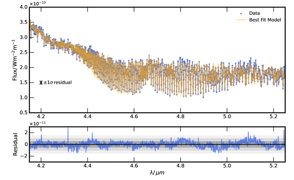
Figure 1: Top Panel: Best fitting model from the retrieval, along with the data points of the NIRSpec G395H/F290LP detector 2 (NRS2) observations of VHS 1256 b. We also show the 1$\sigma$ range of the residuals of the data and model. Bottom Panel: Residuals of the best fit model and the observations, with the 1, 2 and 3$\sigma$ ranges shown in grey.

In this work we retrieve the spectrum of VHS J125601.92–125723.9 b (hereafter VHS 1256 b), a directly-imaged companion, also called a super-Jupiter, that straddles the brown dwarf/planet boundary (Gauza et al., 2015; Dupuy et al., 2023) at the edge of the L/T transition. We use data from the JWST early release science programme (ERS 1386, PI Hinkley) (Miles et al., 2023), performing spectral retrievals of the G395H/F290LP NRS 2 observations which cover the 4.1-5.3 $\mu$m wavelength range. We explore the isotopic ratios of CO by separately retrieving the chemical abundances of ¹²C¹⁶O, ¹³C¹⁶O, ¹²C¹⁸O and ¹²C¹⁷O, in addition to H₂O, CO₂, CH₄ and NH₃. In particular, ¹²C/¹³C is an important quantity given that it has shown some variation between exoplanets and brown dwarfs (Zhang et al., 2021a) and shows differences between the Solar System and the local inter-stellar medium (ISM; Wilson, 1999; Milam et al., 2005).

The next section discusses the retrieval setup, followed by the results, and finally we present the discussion and conclusions of our work.

2 Atmospheric Retrieval

We perform our atmospheric retrieval with HyDRA (Gandhi & Madhusudhan, 2018; Gandhi et al., 2023), modified to allow for the characterisation of non-irradiated exoplanets, as discussed below. We use the JWST NIRSpec IFU G395H/F290LP dataset of VHS 1256 b (Miles et al., 2023), covering the $\sim$4.1-5.3 $\mu$m wavelength range of NRS2. This is the wavelength range where CO and all of its isotopologues have prominent opacity. In addition, CO has well separated spectral lines which are resolvable at the R$\sim$2,700 spectral resolution of the observations, and the ¹²C¹⁶O absorption lines are clearly visible in the observed spectrum shown in Figure 1. Henceforth, unless otherwise stated, we refer to ¹²C and ¹⁶O as C and O respectively, as these are the primary isotopes of each species.

Table 1: Temperature and pressure grid for the cross sections for each species.

T(K)	300	400	500	600	700	800
	900	1000	1200	1400	1600	1800
	2000	2500	3000	3500	4000
P(bar)	$10^{-5}$	$10^{-4}$	$10^{-3}$	$10^{-2}$	$10^{-1}$	1
	10	100

2.1 Molecular cross sections

We retrieve the chemical abundances of CO (main isotopologue), ¹³CO, C¹⁸O, C¹⁷O, H₂O, CO₂, CH₄ and NH₃. The CO isotopologues all have differing cross sections as their line positions are shifted given the differing masses of the carbon and oxygen atoms. Hence each isotopologue is independently distinguishable in the spectrum given sufficient spectral resolution and signal-to-noise. We use the main isotopologue only for species other than CO, with the exception of CH₄, where we include the opacity for all isotopologues weighted by their terrestrial abundances. We use line lists from ExoMol (Tennyson et al., 2016) for H₂O (Polyansky et al., 2018) and NH₃ (Coles et al., 2019), HITEMP for the CO isotopologues (Rothman et al., 2010; Li et al., 2015) and CH₄ (Hargreaves et al., 2020), and Ames for CO₂ (Huang et al., 2013, 2017). We calculate the molecular cross section of each species on a grid of pressure and temperature (see Table 1), with each line broadened by applying a Voigt profile given the H₂/He broadening coefficients. Further details of the cross section calculations can be found in Gandhi et al. (2020). We set the vertically constant volume mixing ratios of each species as a free parameter in the retrieval, resulting in eight free parameters for the chemical composition of the atmosphere. Vertically constant abundances are justified given that the abundances of H₂O and CO are not expected to vary significantly with pressure, and because observations from other similar targets have shown that vertically-varying chemistry such as with chemical equilibrium models do not necessarily provide as good a fit as those with free chemistry (de Regt et al., 2023). In addition to the molecular opacity, we also include absorption from H₂-H₂ and H₂-He collisionally induced absorption (Richard et al., 2012).

2.2 P-T profile

We parametrise the P-T profile according to the method in de Regt et al. (2023), with 9 P-T knots, spaced such that grid points are more frequent in the photosphere region between 10-0.1 bar (see Figure 2). This ensures that there are a sufficient number of knots to cover the full atmosphere but keeps their overall number to a minimum in the regions where the spectrum is less sensitive. To prevent oscillatory behaviour, the general P-splines formalism of Li & Cao (2022) is employed to compute a log-likelihood penalty as

$$\ln\mathcal{L}_{\mathrm{penalty}}=-\frac{\mathrm{PEN}^{(3)}_{\mathrm{gps}}}{2\gamma}-\frac{1}{2}\ln(2\pi\gamma).$$ (1)

Here, $\mathrm{PEN}^{(3)}_{\mathrm{gps}}$ is the third-order general difference penalty which increases for larger temperature variations at the P-T knots. Additionally, temperature variations are penalised more severely for smaller knot separations in log pressure. Similar to Line et al. (2015), the factor $\gamma$ is a retrieved parameter that scales the contribution of the penalty to the overall log-likelihood, thereby allowing for more oscillations if the data warrants it. In total, 10 free parameters are utilised for the P-T profile. The temperature profile used to generate the planetary spectrum incorporates 50 layers between 100-10^-6 bar evenly spaced in log pressure.

	Parameter	Prior Range
Chemistry	$\log(\mathrm{H_{2}O})$	-12 $\rightarrow$ -1
	$\log(\mathrm{{}^{12}CO})$	-12 $\rightarrow$ -1
	$\log(\mathrm{{}^{13}CO})$	-12 $\rightarrow$ -1
	$\log(\mathrm{C^{18}O})$	-12 $\rightarrow$ -1
	$\log(\mathrm{C^{17}O})$	-12 $\rightarrow$ -1
	$\log(\mathrm{CO_{2}})$	-12 $\rightarrow$ -1
	$\log(\mathrm{CH_{4}})$	-12 $\rightarrow$ -1
	$\log(\mathrm{NH_{3}})$	-12 $\rightarrow$ -1
Temp. Profile	$T_{\mathrm{100bar}}$ / K	300 $\rightarrow$ 4000
	$T_{\mathrm{10bar}}$ / K	300 $\rightarrow$ 4000
	$T_{\mathrm{3bar}}$ / K	300 $\rightarrow$ 4000
	$T_{\mathrm{1bar}}$ / K	300 $\rightarrow$ 4000
	$T_{\mathrm{0.3bar}}$ / K	300 $\rightarrow$ 4000
	$T_{\mathrm{0.1bar}}$ / K	300 $\rightarrow$ 4000
	$T_{\mathrm{0.01bar}}$ / K	300 $\rightarrow$ 4000
	$T_{\mathrm{10^{-4}bar}}$ / K	300 $\rightarrow$ 4000
	$T_{\mathrm{10^{-6}bar}}$ / K	300 $\rightarrow$ 4000
P-T penalty	$\log(\gamma)$	-3 $\rightarrow$ 2
Planet param.	$\mathrm{R_{p}/R_{J}}$	0.6 $\rightarrow$ 2.5
	$\log(\mathrm{g/cms^{-2}})$	3.5 $\rightarrow$ 5.5
Clouds/hazes	$\log(\kappa_{\mathrm{4.1\mu m}}/\mathrm{cm^{2}g^{-1}})$	-10 $\rightarrow$ 2
	$\log(\kappa_{\mathrm{5.3\mu m}}/\mathrm{cm^{2}g^{-1}})$	-10 $\rightarrow$ 2
	$\log(P_{\mathrm{cl}}/\mathrm{bar})$	-4 $\rightarrow$ 2
	$\log(\alpha_{\mathrm{cl}})$	0 $\rightarrow$ 20
	$\log(\beta_{\mathrm{err}})$	-1 $\rightarrow$ 2
	$\Delta V_{\mathrm{sys}}$ / kms-1	-30 $\rightarrow$ 30
	resolution	1500 $\rightarrow$ 5000
	$f_{\lambda}$	0.7 $\rightarrow$ 1.3

Table 2: Parameters and uniform prior ranges for our retrieval of VHS 1256 b.

2.3 Retrieval Setup

In addition to the chemical abundances and temperature profile parameters, we retrieve the planetary radius, log gravity, the spectral resolution of the observations, planetary velocity shift, an error scale factor and a wavelength-dependent model scale factor. The error scale factor, $\beta_{\mathrm{err}}$ allows for a scaling of all of the error bars of the data points. The overall likelihood per model is determined as

$$\log(\mathcal{L})= -\frac{1}{2}\sum_{i}\Big{(}\frac{d_{i}-m_{i}}{\beta_{\mathrm{err}}\sigma_{i}}\Big{)}^{2}-\frac{1}{2}\sum_{i}\ln(2\pi(\beta_{\mathrm{err}}\sigma_{i})^{2})$$ (2)

$$+\ln\mathcal{L}_{\mathrm{penalty}},$$

where $d_{i}$ and $m_{i}$ refer to the data and model for each point $i$, and $\sigma_{i}$ represents the uncertainty of each data point.

The wavelength-dependent model scale factor, $f_{\lambda}$, scales the model linearly with the wavelength relative to the blue end of the spectrum. The scaled spectrum used in the retrieval is given by

$$F_{\mathrm{scaled}}(\lambda)=F_{\mathrm{unscaled}}(\lambda)\Big{(}1+\frac{\lambda-4.1~{}\mathrm{\mu m}}{5.3~{}\mathrm{\mu m}-4.1~{}\mathrm{\mu m}}f_{\lambda}\Big{)}.$$ (3)

This new approach was implemented given the high signal-to-noise of the observations, and allows flexibility for any gradients in the spectrum that cannot be well modelled and/or any systematics in the spectrum. In addition, the spectral resolution of the observations varies with wavelength, and such a formulation allows some flexibility of the model to account for this. For instance, an increasing spectral resolution with wavelength would be compensated by a positive value for $f_{\lambda}$, as the redder wavelengths are more highly weighted in the convolution.

We also retrieve a non-grey cloud deck through four additional parameters, with cloud opacities set at 4.1 and 5.3 $\mu$m and interpolated at wavelengths in between, as well as a cloud deck pressure, $P_{\mathrm{cl}}$, and pressure-dependent power-law, $\alpha_{\mathrm{cl}}$ (see e.g., Mollière et al., 2020; de Regt et al., 2023). Clouds have been shown to be significant in this target (Miles et al., 2023), and our cloud model ensures the cloud deck is sufficiently flexible to account a range of cloud deck pressures as well as any wavelength dependent variation in its opacity across the $\sim$1.2 $\mu$m range of the observations.

Overall, the retrieval therefore includes 28 free parameters, with eight for the volume mixing ratio of each chemical species (including the CO isotopologues) and nine for the P-T profile, with an additional penalty scale factor (see Table 2). Our prior ranges were chosen to allow the retrieval to explore a wide range of potential solutions for the atmosphere, and ensured that none of the parameters converged to the edge of the prior range. Note however that the choice of prior range does impact the overall evidence. For the detection significances, we removed the specific free parameter of the volume mixing ratio of the given species, and ensured that the other parameters in the retrieval were left with the same prior. Each model is generated at a spectral resolution of R=100,000, before being convolved by a Gaussian profile to the spectral resolution of the observations (a free parameter in our retrieval). We perform the retrievals with MultiNest (Feroz & Hobson, 2008; Feroz et al., 2009; Buchner et al., 2014). We also perform additional retrievals by removing each species at a time for the leave-one-out cross-validation tests (see section 3.1.1) and in order to determine the detection significances of each species.

3 Results

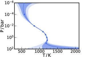
Figure 2: Retrieved pressure-temperature profile form the retrieval of VHS 1256 b. The solid line shows the median values and the dark and light shaded regions indicate the 1 and 2$\sigma$ uncertainties respectively. The markers indicate the P-T knots used in the retrieval (see section 2.2).

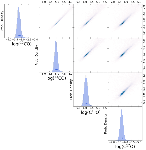
Figure 3: Posterior distributions of the volume mixing ratios of the isotopologues of CO in the retrieval of VHS 1256 b. These show the dependence of one species on the other. Note that C and O refer to the main isotopologues, ¹²C and ¹⁶O, respectively.

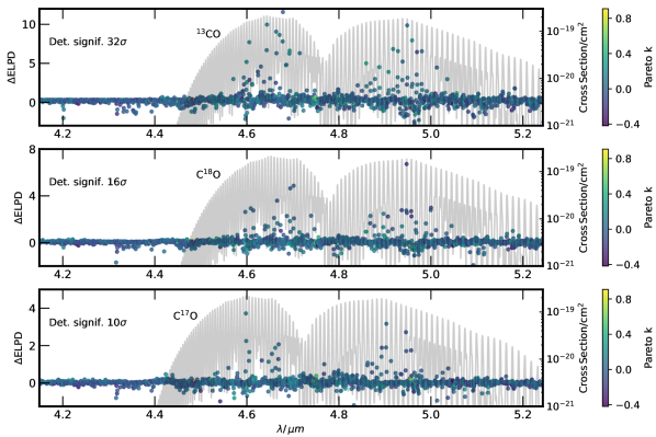
Figure 4: Difference in the expected log posterior predictive density (ELPD) for each isotopologue against our fiducial model. A positive $\Delta\mathrm{ELPD}$ score indicates that the model with the isotopologue is preferred by that data point. The colour bar indicates the Pareto k values for each of the data points, with points $\lesssim$ 0.7 indicating a good PSIS approximation (see section 3.1.1). The vast majority of the data points fall into this category and hence our use of the leave-one-out cross-validation is robust for all three isotopologues. In grey we also show the molecular cross section for each of the isotopologues at 1 bar pressure and 1200 K temperature at the spectral resolution of the observations (R$=$2,700).

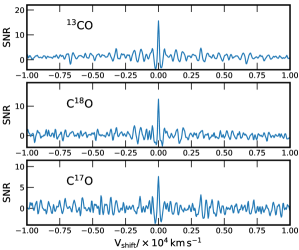
Figure 5: Signal-to-noise ratio (SNR) derived from the cross-correlation functions of the CO isotopologues.

Figure 1 shows the best fit retrieved spectrum to the observations and its residuals. Overall, this shows a good fit to the data, with the residuals only showing some low order deviations in the 4.8-5.1 $\mu$m range. The residuals may arise due to other species present in the atmosphere which are not accounted for in our retrieval, potentially even other isotopologues of molecules such as H₂O and CO₂. Generally however, the model shows a good fit, in particular for the clearly visible ¹²CO lines, as well as the H₂O and CO₂ features which are more prominent in the bluer regions of the spectrum, confirming the detections from Miles et al. (2023).

The retrieved P-T profile is shown in Figure 2, and indicates a generally increasing temperature with pressure, as expected for non-irradiated objects. However, we do see that the temperature profile has a very slight inverted profile at $\sim$10 bar, which is near the edge of the photosphere where the continuum is set. This is likely because there may be additional species that we have not accounted for which is degenerate with the P-T profile of the atmosphere, for instance arising from other trace species or isotopes of CO₂ and H₂O. Overall though the temperature profile is consistent with expectations for such objects near the L/T transition and the photospheric temperature of $\sim$1100 K agrees well with previous works (Zhou et al., 2020; Hoch et al., 2022; Petrus et al., 2023; Miles et al., 2023).

3.1 CO Isotopologues

We constrain the chemical abundances of ¹²CO, the primary isotopologue of CO, as well as the minor isotopes ¹³CO, C¹⁸O and C¹⁷O, as shown in Figure 3. The isotopologues are distinguishable given that their opacities differ at the R$\sim$2,700 resolution of the observations. There is a strong interdependence between species, common from previous observations of such targets (e.g., Line et al., 2015; Burningham et al., 2017; Piette & Madhusudhan, 2020). This highlights that the absolute abundances of each species may not be as well constrained, but we find that their ratios are significantly more precise and robust, as also seen with ground-based high-resolution spectroscopy (Gibson et al., 2022; Gandhi et al., 2023; Pelletier et al., 2023). The less prominent isotopologues, C¹⁸O and C¹⁷O, show the weakest correlation given their lower abundances. This first detection of C¹⁸O and C¹⁷O in an exoplanet atmosphere demonstrates how the high quality JWST spectra can constrain minor isotopes.

3.1.1 Robustness Tests

We ensured that our constraints were robust through performing a Bayesian leave-one-out cross-validation (Welbanks et al., 2023). This method fits a model to the full data with each data point removed by determining the expected log posterior predictive density (ELPD). Comparing with ELPD scores of a model with and without a given isotopologue therefore allows us to determine which data points most strongly prefer the isotopologue. Note that in principle a separate retrieval would need to be performed for every single data point, but we use the Pareto Smoothed Importance Sampling (PSIS) (Vehtari et al., 2017). The Pareto k distribution fitted to the distribution of importance weights is a measure of how much the posterior changes with the removal of a single data point. Typically, Pareto k values $\lesssim$0.7 are a good approximation, but data points with values $>$0.7 will generally require a full retrieval without that point to fully assess the effect of removing it on the posterior.

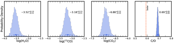
Figure 6: Marginalised posterior distributions for the volume mixing ratios of H₂O, ¹²CO, CO₂ and the overall atmospheric C/O ratio (right panel) from the retrieval of the $\sim$4.1-5.3 $\mu$m JWST observations of VHS 1256 b. The red dashed line shows the solar C/O ratio (Asplund et al., 2021).

Figure 4 shows the $\Delta\mathrm{ELPD}$ and Pareto k values for each data point, with high $\Delta\mathrm{ELPD}$ values indicating that this data point prefers a model with the isotopologue. For all three of the isotopologues we find that the region of the spectrum where the detections are most influenced are the regions where each species has strong opacity. In addition, each isotopologue detection is driven by numerous data points, and the vast majority of the data points have Pareto k values $<$0.7, indicating a good approximation with PSIS. Therefore, each of our detections are robust. Note that not all of the wavelengths where the isotopologues have features have high $\Delta\mathrm{ELPD}$ values as other species such as H₂O, CO₂ and ¹²C¹⁶O have stronger features and therefore interfere with the isotopologue signals at some wavelengths. We determine the detection significances of each isotopologue through comparison of the Bayesian evidence of retrievals performed without each. We detect ¹³CO, C¹⁸O and C¹⁷O very strongly, at significances of 32$\sigma$, 16$\sigma$ and 10$\sigma$ respectively. In addition, the error scale factor was increased when the isotopologues were not included in the retrieval, with the retrievals without ¹³CO, C¹⁸O and C¹⁷O showing increases of 37%, 6% and 4% respectively. Hence, not including these species is a worse fit to the observations and thus requires a larger scaling of the error bars in order to match the model to the data.

We performed retrievals with a high pass filter applied to the data, which removes low order variability in the spectrum and ensures that the fit is performed on the spectral lines and their strengths only. This is particularly important to test as there is some low order deviations between the data and the best fit model in Figure 1. To achieve this we used a running median of 20 data points on the observations and for every model in the retrieval. We found no significant change to any of the isotope ratios, and the detection significances remained similar, at 31$\sigma$, 15$\sigma$ and 10$\sigma$ for ¹³CO, C¹⁸O and C¹⁷O respectively.

In addition to these tests, we also detected each of the isotopologues through cross-correlation, as shown in Figure 5. Esparza-Borges et al. (2023) showed that this technique is applicable to JWST observations by detecting CO in the transiting exoplanet WASP-39 b with NIRSpec observations. We follow the procedure of Zhang et al. (2021a), using the data residuals (data subtracted by the best-fit model without the particular species) with a model spectral template, calculated by subtraction of the best-fit model without the species from the best-fit model with all species. Both the data residuals and the model template are then high-pass filtered and cross-correlated. We determine the signal-to-noise by dividing the cross-correlation by its standard deviation and subtracting off the mean. Our signal-to-noise ratios for all three isotopologues are lower than their detection significances, most likely due to aliasing with the periodic CO lines, but other factors such as the under-sampling of the peak signal due to the wavelength spacing of the data points may also reduce the overall signal. Nevertheless, the detections of ¹³CO and the oxygen isotopologues, C¹⁸O and C¹⁷O, remains clearly visible over the noise.

3.2 Other molecular species

In addition to CO and its various isotopologues, we also constrain H₂O and CO₂ (primary isotopologues only) given their strong opacity in this range, with their marginalised volume mixing ratios shown in Figure 6. We detect H₂O with a lower abundance than the ¹²CO by $\sim 0.34$ dex, and hence the atmospheric C/O ratio is $0.69^{+0.01}_{-0.01}$. This is consistent with previous works (Hoch et al., 2022; Petrus et al., 2023). Note that, as before, the ratio is better constrained than the absolute abundances of H₂O and CO. The C/O ratio is higher than the solar value of 0.59 (Asplund et al., 2021), but some oxygen may have condensed out in silicates (Burrows & Sharp, 1999), which will raise the measured atmospheric C/O value.

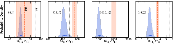
Figure 7: Isotope ratios ¹²C/¹³C, ¹⁶O/¹⁸O, ¹⁶O/¹⁷O and ¹⁸O/¹⁷O derived from the CO abundances of VHS 1256 b. The red dashed line and shaded area show the value measured for the local inter-stellar medium (ISM) and its 1$\sigma$ uncertainty (Wilson, 1999; Milam et al., 2005), and the dotted black line shows the value for the Solar System.

The CO₂ abundance is much lower at $\log(\mathrm{CO_{2}})=-6.88^{+0.12}_{-0.12}$, but its detection significance of 28$\sigma$ remains high given its very strong opacity at $\sim$4.2 $\mu$m. This confirms the results by Miles et al. (2023), who showed that the addition of CO₂ opacity improved the spectral fit to these JWST observations of VHS 1256 b. Carbon dioxide has been detected in a range of late-L to T-dwarfs (e.g., Sorahana & Yamamura, 2012) and is an excellent proxy for the metallicity, as it increases non-linearly with the overall metal content of the atmosphere in chemical equilibrium (e.g., Madhusudhan, 2012; Moses et al., 2013). Our constrained abundance indicates an atmosphere that is at or near solar metallicity. We note however that the CO₂ abundance may be a strong function of the atmospheric pressure for such objects (Lodders & Fegley, 2002), and our assumption of a vertically independent volume mixing ratio may therefore break down if the vertical mixing is weak.

We also retrieve the CH₄ and NH₃ abundances, but find only upper limits of $\log(\mathrm{CH_{4}})<-6.2$ and $\log(\mathrm{NH_{3}})<-6.8$ at 2$\sigma$ confidence as these species do not possess strong opacity a these wavelengths. Other wavelengths such as the $\sim$3-4 $\mu$m range have shown that CH₄ is present in the atmosphere, which has also indicated that the atmosphere is in chemical disequilibrium (Miles et al., 2018, 2023). However, the CH₄ is lower abundance than the CO and hence will not significantly alter C/O estimates.

4 Discussion and Conclusions

We have constrained the ¹³C, ¹⁸O and ¹⁷O isotopes from the CO abundances for the directly imaged companion VHS 1256 b through retrievals of the JWST NIRSpec G395H/F290LP observations in the 4.1-5.3 $\mu$m range (Miles et al., 2023). Figure 7 shows the isotope ratios for ¹²C/¹³C, ¹⁶O/¹⁸O, ¹⁶O/¹⁷O and ¹⁸O/¹⁷O. These ratios are more precise and robust than the absolute abundances, as discussed in section 3.1. All of the ratios have median values which are lower than for the ISM and Solar System, but the ¹²C/¹³C ratio is still within the 1$\sigma$ uncertainty of the local ISM value (Milam et al., 2005). The ratios are also lower than ¹²C/¹³C and ¹⁶O/¹⁸O values measured for an M-dwarf binary (Crossfield et al., 2019). Our ¹²C/¹³C value is in between the value of $\sim$30 obtained for planetary companions YSES-1 b and WASP-77 A b (Zhang et al., 2021b; Line et al., 2021) and the value of $\gtrsim$100 constrained for isolated brown dwarfs (Zhang et al., 2021a; de Regt et al., 2023).

Constraining the carbon and oxygen isotopes in an exoplanet atmosphere is key as isotope fractionation processes in protoplanetary disks can drive differences in their abundances. Several key processes can alter their ratios during planetary formation. Firstly, isotopologue selective photodissociation will prevent the more abundant isotopologues from dissociating because their higher column density will prevent stellar UV photons penetrating deep into a protoplanetary disk (e.g., Visser et al., 2009). The less prominent isotopes will not be as effectively shielded and will therefore be more dissociated, resulting in the gas-phase ratios of more abundant isotopes to less abundant isotopes increasing. Secondly, the gas and ice phase interactions of CO can lead to isotopologue partitioning, as has been shown for ¹²C/¹³C ratios (Smith et al., 2015). Furthermore, isotope ion exchange reactions can increase the gas phase ¹³CO in protoplanetary disks, but generally does not have a strong impact on the oxygen isotopes (Langer et al., 1984). A higher excitation temperature of ¹²CO than ¹³CO can also provide differences in the isotopologue ratio of these two species (Goto et al., 2003).

Through this work we have been able to constrain the minor oxygen isotopes in a Super Jupiter for the first time. The ¹⁸O and ¹⁷O are lower abundance than ¹³C, but their ratios are still well constrained given the high precision and signal-to-noise observations. Both the ¹⁸O and ¹⁷O are more abundant than expected, with the ¹⁶O/¹⁸O and ¹⁶O/¹⁷O ratios lower than for the local ISM and Solar System values. This could be due to ices richer in the weaker isotopes being accreted during formation, potentially driven by isotope selective photodissociation. Any photodissociation of the gas phase would increase the ratio, which goes against our low retrieved ratios. A previous hint of C¹⁸O in a brown dwarf indicated a ¹⁶O/¹⁸O ratio nearer to $\sim$1500 (Zhang et al., 2022), higher than our constrained value. This could be a potential indication of chemical inhomogeneity of molecular clouds between planetary systems. If protoplanetary disks form from evolved intermediate mass stars, the systems may be more enhanced in minor isotopes.

The ratio of the minor oxygen isotopes, ¹⁸O/¹⁷O, is also lower, with our value more akin to that of the galactic centre. In addition to potential isotope fractionation processes, the enhanced ¹⁷O in VHS 1256 b may be an indication of accretion of material from lower mass stars, which are expected to be richer in this isotope (Wouterloot et al., 2008). Note however that the ¹⁷O constraint from our work is the lowest abundance and the weakest detection significance, and therefore may not be as reliable as those for the other isotopes. In addition, VHS 1256 b shows significant time variability (Zhou et al., 2022), which is most likely to affect our abundance constraints for the weaker species.

Our findings highlight the power of JWST to determine isotope ratios in exoplanetary atmospheres. The highly robust detections of both carbon and oxygen isotopologues of CO at very high significances demonstrate how we can expand atmospheric science into new avenues in planetary formation through isotopic chemistry. In the future, we may be able to extend this to determine D/H ratios for exoplanet atmospheres, which is an excellent tracer for planet formation (Morley et al., 2019) as well as the evolution of targets near the deuterium-burning mass boundary (Dupuy et al., 2023). However, this is challenging as deuterium is typically $\sim 10^{4}\times$ less abundant than ¹H, and high accuracy and high temperature line lists for deuterium-rich species are required (e.g., Voronin et al., 2010). We may additionally be able to constrain isotopic ratios for close-in transiting planets, thereby providing a contrast between hot Jupiters and the more widely separated planet populations. Another important insight will be comparison of the isotope ratios in host stars to determine whether differences in exoplanetary atmospheric ratios are caused by isotope fractionation or intrinsic differences in initial formation chemistry. This will also set the stage for the next generation of facilities such as the Extremely Large Telescope (ELT), with instruments such as METIS (Brandl et al., 2021) and ANDES (Maiolino et al., 2013) capable of very high precision and spectral resolution atmospheric observations in the coming decade.

References

- Alderson et al. (2023) Alderson, L., Wakeford, H. R., Alam, M. K., et al. 2023, Nature, 614, 664, doi: 10.1038/s41586-022-05591-3
- Asplund et al. (2021) Asplund, M., Amarsi, A. M., & Grevesse, N. 2021, A&A, 653, A141, doi: 10.1051/0004-6361/202140445
- Brandl et al. (2021) Brandl, B., Bettonvil, F., van Boekel, R., et al. 2021, The Messenger, 182, 22, doi: 10.18727/0722-6691/5218
- Buchner et al. (2014) Buchner, J., Georgakakis, A., Nandra, K., et al. 2014, A&A, 564, A125, doi: 10.1051/0004-6361/201322971
- Burningham et al. (2017) Burningham, B., Marley, M. S., Line, M. R., et al. 2017, MNRAS, 470, 1177, doi: 10.1093/mnras/stx1246
- Burrows & Sharp (1999) Burrows, A., & Sharp, C. M. 1999, ApJ, 512, 843, doi: 10.1086/306811
- Chilcote et al. (2017) Chilcote, J., Pueyo, L., De Rosa, R. J., et al. 2017, AJ, 153, 182, doi: 10.3847/1538-3881/aa63e9
- Coles et al. (2019) Coles, P. A., Yurchenko, S. N., & Tennyson, J. 2019, MNRAS, 490, 4638, doi: 10.1093/mnras/stz2778
- Constantinou et al. (2023) Constantinou, S., Madhusudhan, N., & Gandhi, S. 2023, ApJ, 943, L10, doi: 10.3847/2041-8213/acaead
- Crossfield et al. (2019) Crossfield, I. J. M., Lothringer, J. D., Flores, B., et al. 2019, ApJ, 871, L3, doi: 10.3847/2041-8213/aaf9b6
- de Regt et al. (2023) de Regt, S., Snellen, I., & Gandhi, S. 2023, A&A, in prep
- Dupuy et al. (2023) Dupuy, T. J., Liu, M. C., Evans, E. L., et al. 2023, MNRAS, 519, 1688, doi: 10.1093/mnras/stac3557
- Esparza-Borges et al. (2023) Esparza-Borges, E., López-Morales, M., Adams Redai, J. I., et al. 2023, ApJ, 955, L19, doi: 10.3847/2041-8213/acf27b
- Feroz & Hobson (2008) Feroz, F., & Hobson, M. P. 2008, MNRAS, 384, 449, doi: 10.1111/j.1365-2966.2007.12353.x
- Feroz et al. (2009) Feroz, F., Hobson, M. P., & Bridges, M. 2009, MNRAS, 398, 1601, doi: 10.1111/j.1365-2966.2009.14548.x
- Gandhi & Madhusudhan (2018) Gandhi, S., & Madhusudhan, N. 2018, MNRAS, 474, 271, doi: 10.1093/mnras/stx2748
- Gandhi et al. (2020) Gandhi, S., Brogi, M., Yurchenko, S. N., et al. 2020, MNRAS, 495, 224, doi: 10.1093/mnras/staa981
- Gandhi et al. (2023) Gandhi, S., Kesseli, A., Zhang, Y., et al. 2023, AJ, 165, 242, doi: 10.3847/1538-3881/accd65
- Gaudi et al. (2020) Gaudi, B. S., Seager, S., Mennesson, B., et al. 2020, arXiv e-prints, arXiv:2001.06683, doi: 10.48550/arXiv.2001.06683
- Gauza et al. (2015) Gauza, B., Béjar, V. J. S., Pérez-Garrido, A., et al. 2015, ApJ, 804, 96, doi: 10.1088/0004-637X/804/2/96
- Gibson et al. (2022) Gibson, N. P., Nugroho, S. K., Lothringer, J., Maguire, C., & Sing, D. K. 2022, MNRAS, 512, 4618, doi: 10.1093/mnras/stac091
- Goto et al. (2003) Goto, M., Usuda, T., Takato, N., et al. 2003, ApJ, 598, 1038, doi: 10.1086/378978
- Grant et al. (2023) Grant, D., Lothringer, J. D., Wakeford, H. R., et al. 2023, ApJ, 949, L15, doi: 10.3847/2041-8213/acd544
- Hargreaves et al. (2020) Hargreaves, R. J., Gordon, I. E., Rey, M., et al. 2020, ApJS, 247, 55, doi: 10.3847/1538-4365/ab7a1a
- Hoch et al. (2022) Hoch, K. K. W., Konopacky, Q. M., Barman, T. S., et al. 2022, AJ, 164, 155, doi: 10.3847/1538-3881/ac84d4
- Huang et al. (2013) Huang, X., Freedman, R. S., Tashkun, S. A., Schwenke, D. W., & Lee, T. J. 2013, J. Quant. Spec. Radiat. Transf., 130, 134, doi: 10.1016/j.jqsrt.2013.05.018
- Huang et al. (2017) Huang, X., Schwenke, D. W., Freedman, R. S., & Lee, T. J. 2017, Journal of Quantitative Spectroscopy and Radiative Transfer, 203, 224 , doi: https://doi.org/10.1016/j.jqsrt.2017.04.026
- Janson et al. (2013) Janson, M., Brandt, T. D., Kuzuhara, M., et al. 2013, ApJ, 778, L4, doi: 10.1088/2041-8205/778/1/L4
- JWST Transiting Exoplanet Community Early Release Science Team et al. (2023) JWST Transiting Exoplanet Community Early Release Science Team, Ahrer, E.-M., Alderson, L., et al. 2023, Nature, 614, 649, doi: 10.1038/s41586-022-05269-w
- Langer et al. (1984) Langer, W. D., Graedel, T. E., Frerking, M. A., & Armentrout, P. B. 1984, ApJ, 277, 581, doi: 10.1086/161730
- Lavie et al. (2017) Lavie, B., Mendonça, J. M., Mordasini, C., et al. 2017, AJ, 154, 91, doi: 10.3847/1538-3881/aa7ed8
- Lee et al. (2013) Lee, J.-M., Heng, K., & Irwin, P. G. J. 2013, ApJ, 778, 97, doi: 10.1088/0004-637X/778/2/97
- Li et al. (2015) Li, G., Gordon, I. E., Rothman, L. S., et al. 2015, ApJS, 216, 15, doi: 10.1088/0067-0049/216/1/15
- Li & Cao (2022) Li, Z., & Cao, J. 2022, arXiv e-prints, arXiv:2201.06808, doi: 10.48550/arXiv.2201.06808
- Line et al. (2015) Line, M. R., Teske, J., Burningham, B., Fortney, J. J., & Marley, M. S. 2015, ApJ, 807, 183, doi: 10.1088/0004-637X/807/2/183
- Line et al. (2021) Line, M. R., Brogi, M., Bean, J. L., et al. 2021, Nature, 598, 580, doi: 10.1038/s41586-021-03912-6
- Lodders & Fegley (2002) Lodders, K., & Fegley, B. 2002, Icarus, 155, 393, doi: 10.1006/icar.2001.6740
- Madhusudhan (2012) Madhusudhan, N. 2012, ApJ, 758, 36, doi: 10.1088/0004-637X/758/1/36
- Maiolino et al. (2013) Maiolino, R., Haehnelt, M., Murphy, M. T., et al. 2013, arXiv e-prints, arXiv:1310.3163, doi: 10.48550/arXiv.1310.3163
- Milam et al. (2005) Milam, S. N., Savage, C., Brewster, M. A., Ziurys, L. M., & Wyckoff, S. 2005, ApJ, 634, 1126, doi: 10.1086/497123
- Miles et al. (2018) Miles, B. E., Skemer, A. J., Barman, T. S., Allers, K. N., & Stone, J. M. 2018, ApJ, 869, 18, doi: 10.3847/1538-4357/aae6cd
- Miles et al. (2023) Miles, B. E., Biller, B. A., Patapis, P., et al. 2023, ApJ, 946, L6, doi: 10.3847/2041-8213/acb04a
- Mollière & Snellen (2019) Mollière, P., & Snellen, I. A. G. 2019, A&A, 622, A139, doi: 10.1051/0004-6361/201834169
- Mollière et al. (2020) Mollière, P., Stolker, T., Lacour, S., et al. 2020, A&A, 640, A131, doi: 10.1051/0004-6361/202038325
- Morley et al. (2019) Morley, C. V., Skemer, A. J., Miles, B. E., et al. 2019, ApJ, 882, L29, doi: 10.3847/2041-8213/ab3c65
- Moses et al. (2013) Moses, J. I., Madhusudhan, N., Visscher, C., & Freedman, R. S. 2013, ApJ, 763, 25, doi: 10.1088/0004-637X/763/1/25
- National Academies of Sciences, Engineering, and Medicine (2021) National Academies of Sciences, Engineering, and Medicine. 2021, Pathways to Discovery in Astronomy and Astrophysics for the 2020s (Washington, DC: The National Academies Press), doi: 10.17226/26141
- Pelletier et al. (2023) Pelletier, S., Benneke, B., Ali-Dib, M., et al. 2023, Nature, 619, 491, doi: 10.1038/s41586-023-06134-0
- Petrus et al. (2023) Petrus, S., Chauvin, G., Bonnefoy, M., et al. 2023, A&A, 670, L9, doi: 10.1051/0004-6361/202244494
- Piette & Madhusudhan (2020) Piette, A. A. A., & Madhusudhan, N. 2020, MNRAS, 497, 5136, doi: 10.1093/mnras/staa2289
- Polyansky et al. (2018) Polyansky, O. L., Kyuberis, A. A., Zobov, N. F., et al. 2018, MNRAS, 480, 2597, doi: 10.1093/mnras/sty1877
- Quanz et al. (2022) Quanz, S. P., Ottiger, M., Fontanet, E., et al. 2022, A&A, 664, A21, doi: 10.1051/0004-6361/202140366
- Richard et al. (2012) Richard, C., Gordon, I. E., Rothman, L. S., et al. 2012, J. Quant. Spec. Radiat. Transf., 113, 1276, doi: 10.1016/j.jqsrt.2011.11.004
- Rothman et al. (2010) Rothman, L. S., Gordon, I. E., Barber, R. J., et al. 2010, J. Quant. Spec. Radiat. Transf., 111, 2139, doi: 10.1016/j.jqsrt.2010.05.001
- Samland et al. (2017) Samland, M., Mollière, P., Bonnefoy, M., et al. 2017, A&A, 603, A57, doi: 10.1051/0004-6361/201629767
- Smith et al. (2015) Smith, R. L., Pontoppidan, K. M., Young, E. D., & Morris, M. R. 2015, ApJ, 813, 120, doi: 10.1088/0004-637X/813/2/120
- Sorahana & Yamamura (2012) Sorahana, S., & Yamamura, I. 2012, ApJ, 760, 151, doi: 10.1088/0004-637X/760/2/151
- Tennyson et al. (2016) Tennyson, J., Yurchenko, S. N., Al-Refaie, A. F., et al. 2016, Journal of Molecular Spectroscopy, 327, 73, doi: 10.1016/j.jms.2016.05.002
- The LUVOIR Team (2019) The LUVOIR Team. 2019, arXiv e-prints, arXiv:1912.06219, doi: 10.48550/arXiv.1912.06219
- Todorov et al. (2016) Todorov, K. O., Line, M. R., Pineda, J. E., et al. 2016, ApJ, 823, 14, doi: 10.3847/0004-637X/823/1/14
- Vehtari et al. (2017) Vehtari, A., Gelman, A., & Gabry, J. 2017, Statistics and computing, 27, 1413
- Visser et al. (2009) Visser, R., van Dishoeck, E. F., & Black, J. H. 2009, A&A, 503, 323, doi: 10.1051/0004-6361/200912129
- Voronin et al. (2010) Voronin, B. A., Tennyson, J., Tolchenov, R. N., Lugovskoy, A. A., & Yurchenko, S. N. 2010, MNRAS, 402, 492, doi: 10.1111/j.1365-2966.2009.15904.x
- Welbanks et al. (2023) Welbanks, L., McGill, P., Line, M., & Madhusudhan, N. 2023, AJ, 165, 112, doi: 10.3847/1538-3881/acab67
- Wilson (1999) Wilson, T. L. 1999, Reports on Progress in Physics, 62, 143, doi: 10.1088/0034-4885/62/2/002
- Wouterloot et al. (2008) Wouterloot, J. G. A., Henkel, C., Brand, J., & Davis, G. R. 2008, A&A, 487, 237, doi: 10.1051/0004-6361:20078156
- Zhang et al. (2022) Zhang, Y., Snellen, I. A. G., Brogi, M., & Birkby, J. L. 2022, Research Notes of the American Astronomical Society, 6, 194, doi: 10.3847/2515-5172/ac9309
- Zhang et al. (2021a) Zhang, Y., Snellen, I. A. G., & Mollière, P. 2021a, A&A, 656, A76, doi: 10.1051/0004-6361/202141502
- Zhang et al. (2021b) Zhang, Y., Snellen, I. A. G., Bohn, A. J., et al. 2021b, Nature, 595, 370, doi: 10.1038/s41586-021-03616-x
- Zhou et al. (2022) Zhou, Y., Bowler, B. P., Apai, D., et al. 2022, AJ, 164, 239, doi: 10.3847/1538-3881/ac9905
- Zhou et al. (2020) Zhou, Y., Bowler, B. P., Morley, C. V., et al. 2020, AJ, 160, 77, doi: 10.3847/1538-3881/ab9e04