Breaking matter degeneracy in a model-independent way through the Sunyaev-Zeldovich effect

Abstract

We propose a model-independent Bézier parametric interpolation to alleviate the degeneracy between baryonic and dark matter abundances by means of intermediate-redshift data. To do so, we first interpolate the observational Hubble data to extract cosmic bounds over the (reduced) Hubble constant, $h_{0}$, and interpolate the angular diameter distances, $D(z)$, of the galaxy clusters, inferred from the Sunyaev-Zeldovich effect, constraining the spatial curvature, $\Omega_{k}$. Through the so-determined Hubble points and $D(z)$, we interpolate uncorrelated data of baryonic acoustic oscillations bounding the baryon ($\omega_{b}=h^{2}_{0}\Omega_{b}$) and total matter ($\omega_{m}=h^{2}_{0}\Omega_{m}$) densities, reinforcing the constraints on $h_{0}$ and $\Omega_{k}$ with the same technique. Instead of pursuing the usual treatment to fix $\omega_{b}$ via the value obtained from the cosmic microwave background to remove the matter sector degeneracy, we here interpolate the acoustic parameter from correlated baryonic acoustic oscillations. The results of our Monte Carlo–Markov chain simulations turn out to agree at $1$–$\sigma$ confidence level with the flat $\Lambda$CDM model. While our findings are roughly suitable at $1$–$\sigma$ with its non-flat extension too, the Hubble constant appears in tension up to the $2$–$\sigma$ confidence level. Accordingly, we also reanalyze the Hubble tension with our treatment and find our expectations slightly match local constraints.

I Introduction

In the standard cosmological puzzle, the accelerated expansion of the universe represents a solid evidence, first detected by means of type Ia supernovae (SNe Ia) observations Riess et al. (1998); Perlmutter et al. (1999). The presence of dust under the form of baryons and (cold) dark matter alone is not capable of accelerating the universe today. Accordingly, the acceleration of the universe can be attributed to an exotic dark energy fluid, exerting a repulsive gravitational effect due to its negative equation of state Sahni and Starobinsky (2000); Copeland et al. (2006); Tsujikawa (2011).

The universe energy momentum budget yields a dark energy contributing for $\sim 70\%$, while the remaining $\sim 30\%$ consists of cold dark matter and baryonic matter Planck Collaboration (2020). Within the current cosmological background scenario, the $\Lambda$CDM model, it is not possible to measure separately baryonic matter and cold dark matter by relying solely on SNe Ia observations. This limitation is not only a characteristic of the current cosmological background scenario, where dark energy is under the form of a cosmological constant $\Lambda$ Carroll (2001), but of any dark energy scenario. However, among all possible frameworks, the $\Lambda$CDM model remains the most statistically favored approach to describe the universe large scale dynamics, albeit plagued by conceptual inconsistencies.

Specifically, the $\Lambda$CDM paradigm still suffers from the coincidence and fine-tuning problems Copeland et al. (2006) and cosmological tensions related to the discrepancies in Hubble constant measurements and to the amplitude of the clustering of matter $S_{8}$ using high and low-redshift probes Bernal and Libanore (2023); Di Valentino et al. (2021); Abdalla et al. (2022). To overcome these issues, several theoretical efforts have been made to find alternative models that reproduce the successful features of the $\Lambda$CDM paradigm Luongo and Muccino (2018); D’Agostino et al. (2022); Belfiglio et al. (2022).

From a phenomenological standpoint, diverse model-independent approaches have been proposed in order to estimate the cosmological parameters without assuming a priori the cosmological model Capozziello et al. (2013); Dunsby and Luongo (2016); Luongo and Muccino (2021a, 2023); Shafieloo (2007); Shafieloo and Clarkson (2010); Haridasu et al. (2018).

Motivated by the need of disentangling baryons from cold dark matter, we here propose a model-independent approach based on the Bézier parametric interpolation that: a) approximates the Hubble rate $H(z)$ via the observational Hubble data (OHD) Amati et al. (2019) and constrains the Hubble constant, and b) uses this approximation to interpolate the angular diameter distances $D(z)$ of galaxy clusters, inferred from the Sunyaev-Zeldovich (SZ) effect, to provide bounds on the spatial curvature $\Omega_{k}$. Thus, by virtue of the above extrapolations, we fit both uncorrelated and correlated data sets of baryonic acoustic oscillations (BAO) to constrain the matter densities for baryons $\Omega_{b}$ and for all matter components $\Omega_{m}$, via $\omega_{b}=h_{0}^{2}\Omega_{b}$ and $\omega_{m}=h_{0}^{2}\Omega_{m}$, which the comoving sound horizon, $r_{s}$, depends upon Aizpuru et al. (2021). We point out that the correlated BAO turn out to be essential to break the degeneracy between $\omega_{m}$ and $\omega_{b}$ Efstathiou and Bond (1999), differently of the standard procedure fixing $\omega_{b}$ to cosmic microwave background (CMB) value Planck Collaboration (2020). Accordingly, we intentionally put aside the CMB data from Planck satellite and the Pantheon catalog of SNe Ia Scolnic et al. (2018), due to their tension in determining $h_{0}$. The results of our Monte Carlo–Markov chain (MCMC) simulations, based on the Metropolis-Hastings algorithm, suggest that the matter sector degeneracy is likely alleviated without the need for CMB and/or SNe Ia data. Notably, this technique, while valuable, does not completely eliminate the cosmic tensions that still persist. In fact, in the flat scenario, our $h_{0}$ turns out to be in good agreement with the Planck estimates Planck Collaboration (2020), but still barely consistent with SNe Ia Riess et al. (2022), at $1$–$\sigma$ confidence level, while in the non-flat case, our $h_{0}$ is consistent with Planck only at $2$–$\sigma$ confidence level Planck Collaboration (2020), indicating that spatial curvature may influence the $h_{0}$ measurements. Consequently, when comparing our results with expectations based on the flat (non-flat) $\Lambda$CDM framework, we obtain constraints that are in good agreement with the standard cosmological model at $1$–$\sigma$ ($2$–$\sigma$) level, certifying that the $\Lambda$CDM paradigm is still supported within our treatment.

The paper is structured as follows. In Sect. II, we introduce the data sets and show how to use them to perform model-independent interpolations through Bézier curves. In Sect. III, we show the numerical constraints on $h_{0}$, $\Omega_{k}$, $\omega_{b}$ and $\omega_{m}$, obtained from our MCMC analysis, and compare them with the best-fit parameters inferred from both the flat and the non-flat $\Lambda$CDM models. In Sect. IV, we summarize the physical implications of our efforts, reporting our conclusions and perspectives.

II Methods

To obtain model-independent estimates on the key cosmological parameters, we utilize intermediate redshift catalogs, such as OHD, SZ and BAO data sets. The Pantheon catalog of SNe Ia Scolnic et al. (2018) and CMB data from the Planck satellite Planck Collaboration (2020) are intentionally excluded in view of the existing tension on their estimates on $h_{0}$ Riess et al. (2022); Planck Collaboration (2020).

The model-independent technique here resorted is based on the well-established Bézier parametric interpolation, firstly introduced in Ref. Luongo and Muccino (2021b) and widely adopted in cosmological contexts with promising results Amati et al. (2019); Montiel et al. (2021); Luongo and Muccino (2023); Muccino et al. (2023). We employ this technique to

• interpolate the Hubble rate $H(z)$ from OHD Jimenez and Loeb (2002a),

• use it to derive the angular diameter distance $D(z)$, on which SZ and BAO observables are based, and

• interpolate BAO data to break the baryonic–dark matter degeneracy.

It is worth stressing that the so-interpolated $H(z)$ and $D(z)$ bear no a priori assumptions on $\Omega_{k}$, as long as the data sets do not carry specific priors on it.

II.1 Hubble rate model-independent reconstruction via Bézier polynomials

We interpolate the most updated sample of $N_{\rm O}=33$ Hubble rate measurements, spanning up to the maximum redshift $z_{\rm m}=1.965$ (see Tab. 1). These measurements are determined from spectroscopic measurements of the differences in age $\Delta t$ and redshift $\Delta z$ of couples of passively evolving galaxies (formed at the same time) by resorting the identity $H(z)=-(1+z)^{-1}\Delta z/\Delta t$ Jimenez and Loeb (2002a).

$z$	$H(z)$	Refs.
	(km s-1Mpc-1)
0.0708	$69.0\pm 19.6$	Zhang et al. (2014)
0.09	$69.0\pm 12.0$	Jimenez and Loeb (2002b)
0.12	$68.6\pm 26.2$	Zhang et al. (2014)
0.17	$83.0\pm 8.0$	Simon et al. (2005)
0.179	$75.0\pm 4.0$	Moresco et al. (2012)
0.199	$75.0\pm 5.0$	Moresco et al. (2012)
0.20	$72.9\pm 29.6$	Zhang et al. (2014)
0.27	$77.0\pm 14.0$	Simon et al. (2005)
0.28	$88.8\pm 36.6$	Zhang et al. (2014)
0.352	$83.0\pm 14.0$	Moresco et al. (2016)
0.3802	$83.0\pm 13.5$	Moresco et al. (2016)
0.4	$95.0\pm 17.0$	Simon et al. (2005)
0.4004	$77.0\pm 10.2$	Moresco et al. (2016)
0.4247	$87.1\pm 11.2$	Moresco et al. (2016)
0.4497	$92.8\pm 12.9$	Moresco et al. (2016)
0.47	$89.0\pm 23.0$	Ratsimbazafy et al. (2017)
0.4783	$80.9\pm 9.0$	Moresco et al. (2016)
0.48	$97.0\pm 62.0$	Stern et al. (2010)
0.593	$104.0\pm 13.0$	Moresco et al. (2012)
0.68	$92.0\pm 8.0$	Moresco et al. (2012)
0.75	$98.8\pm 33.6$	Borghi et al. (2022)
0.781	$105.0\pm 12.0$	Moresco et al. (2012)
0.80	$113.1\pm 15.1$	Jiao et al. (2023)
0.875	$125.0\pm 17.0$	Moresco et al. (2012)
0.88	$90.0\pm 40.0$	Stern et al. (2010)
0.9	$117.0\pm 23.0$	Simon et al. (2005)
1.037	$154.0\pm 20.0$	Moresco et al. (2012)
1.3	$168.0\pm 17.0$	Simon et al. (2005)
1.363	$160.0\pm 33.6$	Moresco (2015)
1.43	$177.0\pm 18.0$	Simon et al. (2005)
1.53	$140.0\pm 14.0$	Simon et al. (2005)
1.75	$202.0\pm 40.0$	Simon et al. (2005)
1.965	$186.5\pm 50.4$	Moresco (2015)

Table 1: The redshift distribution (first column) of the OHD measurements with the statistical errors (second column) and the reference papers (third column).

The best-fit, non-linear and monotonic growing function with the redshift of these data is a second order Bézier curve with coefficients $\alpha_{i}$ Amati et al. (2019); Luongo and Muccino (2021b); Montiel et al. (2021); Luongo and Muccino (2023); Muccino et al. (2023), i.e.,

$$H_{2}(z)=g_{\alpha}\sum_{i=0}^{2}\frac{2\alpha_{i}}{i!(2-i)!}\left(\frac{z}{z_{\rm m}}\right)^{i}\left(1-\frac{z}{z_{\rm m}}\right)^{2-i}\,,$$ (1)

where we defined $g_{\alpha}=100\,{\rm km\,s}^{-1}{\rm Mpc}^{-1}$. This interpolated function can be also extrapolated beyond $z_{\rm m}$, to cover the redshift range of the other intermediate redshift probes that will be introduced in the following.

Fitting the OHD measurements with Eq. (1) provides a model-independent estimate of the dimensionless Hubble constant, since at $z=0$ it holds $H_{0}/g_{\alpha}\equiv h_{0}\equiv\alpha_{0}$.

For Gaussian distributed errors $\sigma_{H_{k}}$, the coefficients $\alpha_{i}$ are found by maximizing the log-likelihood function

$$\ln\mathcal{L}_{\rm O}=-\frac{1}{2}\sum_{j=1}^{N_{\rm O}}\left\{\left[\dfrac{H_{j}-H_{2}(z_{j})}{\sigma_{H_{j}}}\right]^{2}+\ln(2\pi\sigma^{2}_{H_{j}})\right\}\,.$$ (2)

II.2 Constraining the curvature with SZ data

The SZ effect is the spectral distortion of the CMB photons via inverse Compton scattering by high-energy electrons gas in galaxy clusters Carlstrom et al. (2002). While CMB photons is observed at microwave frequencies, intra-cluster electrons and their distribution are observed in the X-rays.

Combining the above observations enables the determination, for relatively high threshold signal-to-noise ratio, of the triaxial structure of the clusters and, thus, their morphology-corrected diameter angular distances $D(z)$. A sample of $N_{\rm S}=25$ clusters with such determined distances De Filippis et al. (2005) is listed in Tab. 2.

$z$	$D(z)$
	(Mpc)
$0.023$	$103\pm 42$
$0.058$	$242\pm 61$
$0.072$	$165\pm 45$
$0.074$	$369\pm 62$
$0.084$	$749\pm 385$
$0.088$	$448\pm 185$
$0.091$	$335\pm 70$
$0.142$	$478\pm 126$
$0.176$	$809\pm 263$
$0.182$	$451\pm 189$
$0.183$	$604\pm 84$
$0.202$	$387\pm 141$
$0.202$	$806\pm 163$
$0.217$	$1465\pm 407$
$0.224$	$1118\pm 283$
$0.252$	$946\pm 131$
$0.282$	$1099\pm 308$
$0.288$	$934\pm 331$
$0.322$	$885\pm 207$
$0.327$	$697\pm 183$
$0.375$	$1231\pm 441$
$0.451$	$1166\pm 262$
$0.541$	$1635\pm 391$
$0.550$	$1073\pm 238$
$0.784$	$2479\pm 1023$

Table 2: The sample of galaxy clusters with the redshift (first column) and the diameter angular distances (second column) as inferred from the SZ effect De Filippis et al. (2005).

Using Eq. (1), we obtain an interpolated angular diameter distance defined as

$$D_{2}(z)=\frac{c\left(1+z\right)^{-1}}{g_{\alpha}\alpha_{0}\sqrt{\Omega_{k}}}\sinh\left[\int_{0}^{z}\frac{g_{\alpha}\alpha_{0}\sqrt{\Omega_{k}}dz^{\prime}}{H_{2}(z^{\prime})}\right]\ ,$$ (3)

where $\sinh(\sqrt{\Omega_{k}}x)/\sqrt{\Omega_{k}}$ holds for a curvature parameter $\Omega_{k}>0$, becomes $\sin(\sqrt{|\Omega_{k}|}x)/\sqrt{|\Omega_{k}|}$ for $\Omega_{k}<0$, and reduces to $x$ for $\Omega_{k}=0$.

Again, for Gaussian distributed errors $\sigma_{D_{j}}$, $\alpha_{i}$ and $\Omega_{k}$ can be derived by maximizing the log-likelihood function

$$\ln\mathcal{L}_{\rm S}=-\frac{1}{2}\sum_{j=1}^{N_{\rm S}}\left\{\left[\dfrac{D_{j}-D_{2}(z_{j})}{\sigma_{D_{j}}}\right]^{2}+\ln(2\pi\sigma^{2}_{D_{j}})\right\}\,.$$ (4)

II.3 Constraining the matter density with BAO

In the early universe, BAO are acoustic waves generated by the gravitational interaction between the photon-baryon fluid and inhomogeneities Weinberg (2008). During the drag epoch, baryons decoupled from photons and “froze in” at a scale equal to the sound horizon at the drag epoch redshift $z_{\mathrm{d}}$, i.e., $r_{\mathrm{s}}\equiv r(z_{\mathrm{d}})$. Such a characteristic scale is a standard ruler embedded in the galaxy distribution Cuceu et al. (2019).

A numerically-reconstructed expression for $r_{\mathrm{s}}$, that also includes massive neutrinos, is given by Aizpuru et al. (2021)

$$r_{\mathrm{s}}=\frac{a_{1}~{}e^{a_{2}\left(a_{3}+\omega_{\nu}\right)^{2}}}{a_{4}~{}\omega_{b}^{a_{5}}+a_{6}~{}\omega_{m}^{a_{7}}+a_{8}\left(\omega_{b}\hskip 2.84526pt\omega_{m}\right)^{a_{9}}}~{}\mathrm{Mpc}\,,$$ (5)

and leads to an improvement in the accuracy, over the most used expression Aubourg et al. (2015), of a factor $\sim 3$ in the range within $3\sigma$ of the $\Lambda$CDM best-fit parameters Planck Collaboration (2020), and a factor $\sim 30$ in the broader range Aizpuru et al. (2021). In Eq. (5), the cosmological parameters for baryons $\omega_{b}$ and for both baryonic and dark matter $\omega_{m}$ are free parameters; for massive neutrino species we fixed $\omega_{\nu}=0.000645$ Aubourg et al. (2015). The other coefficients have the following values Aizpuru et al. (2021)

$$\begin{array}[]{lll}a_{1}=0.0034917,&a_{2}=-19.972694,&a_{3}=0.000336186\,,\\ a_{4}=0.0000305,&a_{5}=0.22752,&a_{6}=0.0000314257\,,\\ a_{7}=0.5453798,&a_{8}=374.14994,&a_{9}=4.022356899\,.\\ \end{array}$$

To determine $r_{\mathrm{s}}$ from Eq. (5) requires to break the degeneracy between $\omega_{b}$ and $\omega_{m}$ Efstathiou and Bond (1999). In general, this is achieved by fixing $\omega_{b}$ with the value got from the CMB. However, as stated above, CMB data are intentionally excluded because of the $H_{0}$ tension. Therefore, in the following we work out a procedure, based on different data sets of BAO measurements, that aims not only at providing constraints on $\omega_{b}$ and $\omega_{m}$ (and consequently on $r_{\mathrm{s}}$), but also at reinforcing the constraints on $h_{0}$ and $\Omega_{k}$ got from OHD and SZ data sets, respectively.

Survey	$z$	$\delta(z)$	Refs.
6dFGS	$0.106$	$0.336\pm 0.015$	Beutler et al. (2011)
SDSS-DR7	$0.15$	$0.2239\pm 0.0084$	Ross et al. (2015)
SDSS-DR7	$0.2$	$0.1905\pm 0.0061$	Percival et al. (2010)
SDSS-DR11 LOWZ	$0.32$	$0.1181\pm 0.0023$	Anderson et al. (2014)
SDSS-DR7 LRG	$0.35$	$0.1126\pm 0.0022$	Padmanabhan et al. (2012)
BOSS DR12	$0.38$	$0.1001\pm 0.0011$	Alam et al. (2017)
BOSS DR12	$0.51$	$0.0787\pm 0.0008$	Alam et al. (2017)
SDSS-III/DR9	$0.57$	$0.0726\pm 0.0007$	Anderson et al. (2014)
BOSS DR12	$0.61$	$0.0691\pm 0.0007$	Alam et al. (2017)
SDSS-IV/DR14	$0.72$	$0.0622\pm 0.0016$	Bautista et al. (2018)
SDSS-IV/DR14	$1.52$	$0.0385\pm 0.0015$	Ata et al. (2018)
Survey	$z$	$\Delta(z)$	Refs.
SDSS-III DR8	$0.54$	$9.212\pm 0.410$	Seo et al. (2012)
DECals DR8	$0.697$	$10.387\pm 0.496$	Sridhar et al. (2020)
DES Year1	$0.81$	$10.75\pm 0.43$	Abbott et al. (2019)
DECals DR8	$0.874$	$11.372\pm 0.693$	Sridhar et al. (2020)
Survey	$z$	$\Theta(z)$	Refs.
eBOSS DR16 BAO+RSD	$1.48$	$13.23\pm 0.47$	Hou et al. (2021)
eBOSS DR16	$2.334$	$8.99\pm 0.19$	du Mas des Bourboux et al. (2020)
Survey	$z$	$A(z)$	Refs.
WiggleZ	$0.44$	$0.474\pm 0.034$	Blake et al. (2012)
WiggleZ	$0.6$	$0.442\pm 0.020$	Blake et al. (2012)
WiggleZ	$0.73$	$0.424\pm 0.021$	Blake et al. (2012)

Table 3: The four BAO catalogs with surveys (first column), redshifts (second column), measurements with errors (third column), and references (fourth column).

Tab. 3 lists four kind of BAO data sets. Resorting the interpolations in Eqs. (1) and (3), the first set of $N_{\delta}=11$ measurements is given by the ratio

$$\delta_{2}(z)=\frac{r_{\mathrm{s}}}{[V_{2}(z)]^{1/3}}\,,$$ (6)

where the comoving volume $V_{2}(z)$ is defined as

$$V_{2}(z)=\frac{cz}{H_{2}(z)}\left[(1+z)D_{2}(z)\right]^{2}\,.$$ (7)

From Eqs. (6)–(7), it is clear that such measurements enable constraints on $\omega_{b}$ and $\omega_{m}$ from the definition of $r_{\mathrm{s}}$, on $h_{0}$ from $H_{2}(z)$, and on $\Omega_{k}$ from $D_{2}(z)$.

The second kind of BAO data (see Tab. 3) is a sample of $N_{\Delta}=4$ points described by the interpolated ratio

$$\Delta_{2}(z)=\frac{D_{2}(z)}{r_{\mathrm{s}}}\,,$$ (8)

that constrains $\omega_{b}$ and $\omega_{m}$ from the definition of $r_{\mathrm{s}}$, and $\Omega_{k}$ from $D_{2}(z)$.

The third set of $N_{\Theta}=2$ BAO measurements of Tab. 3 involves the interpolated ratio

$$\Theta_{2}(z)=\frac{c}{r_{\mathrm{s}}H_{2}(z)}\,,$$ (9)

that, besides $\omega_{b}$ and $\omega_{m}$ got from $r_{\mathrm{s}}$, leads to the constraint on $h_{0}$ from $H_{2}(z)$.

Finally, to break the degeneracy between $\omega_{b}$ and $\omega_{m}$, we employ the $N_{A}=3$ correlated BAO measurements Blake et al. (2012) described by the interpolated acoustic parameter

$$A_{2}(z)\equiv g_{\alpha}\frac{\sqrt{\omega_{m}}}{cz}[V_{2}(z)]^{1/3}\,,$$ (10)

that enables constraints on $\omega_{m}$, $h_{0}$, and $\Omega_{k}$.

With the usual assumption of Gaussian distributed errors $\sigma_{X_{j}}$, the log-likelihood functions of the uncorrelated BAO data sets ($X=\delta$, $\Delta$, $\Theta$) are given by

$$\ln\mathcal{L}_{\rm X}=-\frac{1}{2}\sum_{j=1}^{N_{\rm X}}\left\{\left[\dfrac{X_{j}-X_{2}(z_{j})}{\sigma_{X_{j}}}\right]^{2}+\ln(2\pi\sigma^{2}_{X_{j}})\right\}.$$ (11)

Conversely, the log-likelihood function for correlated BAO data with covariance matrix $\mathbf{C}_{\rm B}$ Blake et al. (2012) writes as

$$\ln\mathcal{L}_{\rm A}=-\frac{1}{2}\left[\Delta{\bf A_{2}}^{\rm T}\mathbf{C}_{\rm B}^{-1}\Delta{\bf A_{2}}+\ln\left(2\pi|\det\mathbf{C}_{\rm B}|\right)\right]\,,$$ (12)

where $\Delta{\bf A_{2}}\equiv A_{j}-A_{2}(z_{j})$.

Finally, the total BAO log-likelihood can be written as

$$\ln\mathcal{L}_{\rm B}=\sum_{X}\ln\mathcal{L}_{\rm X}+\ln\mathcal{L}_{\rm A}\,.$$ (13)

III Numerical results

To set the bounds over $\omega_{b}$, $\omega_{m}$, $h_{0}$, and $\Omega_{k}$, we performed an MCMC analysis, based on the Metropolis-Hastings algorithm Metropolis et al. (1953); Hastings (1970), through a modified version of the Wolfram Mathematica free available code presented in Ref. Arjona et al. (2019). We search for the best-fit results that maximize the total log-likelihood function

$$\ln{\mathcal{L}}=\ln{\mathcal{L}_{\rm O}}+\ln{\mathcal{L}_{\rm S}}+\ln{\mathcal{L}_{\rm B}}\,,$$ (14)

with the following priors on the parameters

$$\begin{array}[]{rclcrclr}\alpha_{0}\equiv h_{0}&\in&\left[0,1\right]&&\qquad\Omega_{k}&\in&\left[-2,2\right]&,\\ \alpha_{1}&\in&\left[0,2\right]&&\qquad\omega_{b}&\in&\left[0,1\right]&,\\ \alpha_{2}&\in&\left[0,3\right]&&\qquad\,\,\,\omega_{m}&\in&\left[0,1\right]&.\end{array}$$

The best-fit parameters of our MCMC analysis are listed in Tab. 4 and portrayed in the $1$–$\sigma$ and $2$–$\sigma$ contour plots of Fig. 1, obtained by using a Python free available code Bocquet and Carter (2016). For comparison, Tab. 4 also lists the flat and non-flat $\Lambda$CDM best-fit parameters got from the CMB measurements Planck Collaboration (2020). The best-fitting Bézier curves that interpolate OHD, SZ, and BAO catalogs are portrayed in Fig. 2, where the flat $\Lambda$CDM paradigm (Planck Collaboration, 2020) is also shown for comparison.

	$\alpha_{0}\equiv h_{0}$	$\alpha_{1,2}$	$\Omega_{k}$	$\omega_{b}$	$\omega_{m}$
This work	$0.694_{-0.035\,(-0.055)}^{+0.032\,(+0.054)}$	$1.073_{-0.077\,(-0.123)}^{+0.088\,(+0.140)}$	$-0.08_{-0.52\,(-0.77)}^{+0.52\,(+0.84)}$	$0.0236_{-0.0058\,(-0.0089)}^{+0.0069\,(+0.0118)}$	$0.147_{-0.020\,(-0.031)}^{+0.021\,(+0.034)}$
		$1.973_{-0.076\,(-0.122)}^{+0.079\,(+0.132)}$
$\Lambda$CDM	$0.6736^{+0.0054}_{-0.0054}$	–	–	$0.02237^{+0.00015}_{-0.00015}$	$0.1430^{+0.0011}_{-0.0011}$
$\Lambda$CDM (non-flat)	$0.636^{+0.021}_{-0.023}$	–	$-0.011^{+0.013}_{-0.012}$	$0.02249^{+0.00016}_{-0.00016}$	$0.14099^{+0.0015}_{-0.0015}$

Table 4: Best-fit parameters with $1$–$\sigma$ ($2$–$\sigma$) error bars obtained from the MCMC analysis based on the Bézier interpolation of this work, compared to the flat and non-flat $\Lambda$CDM best-fit parameters Planck Collaboration (2020). In the non-flat $\Lambda$CDM case: a) $\Omega_{k}$ is quoted at $95\%$ limits, whereas the other parameters at $68\%$ limits Planck Collaboration (2020); b) the value of $\omega_{m}$ is calculated by summing up $\omega_{b}$ with the density of cold dark matter, i.e. $\omega_{c}=0.1185^{+0.0015}_{-0.0015}$, and the attached error as the root sum of squares of the errors on $\omega_{b}$ and $\omega_{c}$ Planck Collaboration (2020).

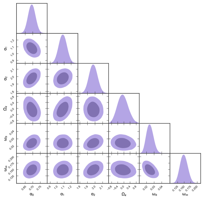
Figure 1: MCMC contour plots of the Bézier interpolation. Darker (lighter) areas exhibit $1$–$\sigma$ ($2$–$\sigma$) confidence regions.

The above results evidence that our interpolation technique of intermediate-redshift data sets is able to set precise model-independent constraints over the key cosmological parameters $\omega_{b}$, $\omega_{m}$, $h_{0}$, and $\Omega_{k}$ listed in Tab. 4. It is immediately clear that these cosmic bounds are in agreement within $1$–$\sigma$ ($2$–$\sigma$) with those got from the flat (non-flat) concordance model, though with larger attached errors. In particular, the Hubble constant tension remains still unsolved, since our value of $h_{0}$ listed in Tab. 4 is still consistent at $1$–$\sigma$ confidence level with the value got from the CMB data ($h_{0}=0.6736\pm 0.0054$) Planck Collaboration (2020) and from SNe Ia ($h_{0}=0.7304\pm 0.0104$) Riess et al. (2022), both obtained in the flat scenario. In the non-flat case, our $h_{0}$ is consistent with Planck only at $2$–$\sigma$ confidence level Planck Collaboration (2020).

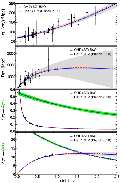
Figure 2: Plots of the best-fitting Bézier curves (blue lines) and $1$–$\sigma$ confidence bands for $H_{2}(z)$, $D_{2}(z)$, $\delta_{2}(z)$, and $\Delta_{2}(z)$ (gray bands), and $A_{2}(z)$ and $\Theta_{2}(z)$ (green bands), compared to the $\Lambda$CDM paradigm (Planck Collaboration, 2020) (dashed red curves).

The spatial curvature found in this work (see Tab. 4) is compatible at $2$–$\sigma$ level with the flat geometry purported by Planck Planck Collaboration (2020). However, the large attached error does not to exclude a priori other geometries. Such a loose constraint is due to scattered and limited redshift span (with respect to the other catalogs here employed) of the SZ data (see second panel in Fig. 2).

IV Final outlooks and perspectives

In this paper, we proposed a novel model-independent technique to extract bounds on the key cosmological parameters, such as the normalized Hubble constant $h_{0}$, the curvature parameter $\Omega_{k}$ and the matter densities $\omega_{b}$, for baryons, and $\omega_{m}$, for all the matter components.

To do so, we resorted a calibration technique based on the well-established Bézier parametric curve and apply it to interpolate the OHD catalog with a second order polynomial curve Amati et al. (2019); Luongo and Muccino (2021b); Montiel et al. (2021); Luongo and Muccino (2023); Muccino et al. (2023), without assuming any a priori cosmological models. Though no assumptions are made, by construction, the interpolating function, $H_{2}(z)$, carries out the valuable constraint on $\alpha_{0}\equiv h_{0}$.

Afterwards, we interpolated other intermediate redshift catalogs, based on the SZ effect measurements and BAO data sets. Recently, SZ data have been used in conjunction with SNe Ia to infer cosmic bounds on $H_{0}$ through the cosmic distance duality relation Colaço et al. (2023). Here, we intentionally excluded SNe Ia Scolnic et al. (2018) and also CMB data Planck Collaboration (2020), mainly because of the existing tension on the values of $h_{0}$ got from these two probes.

Conversely, we used the Hubble rate $H_{2}(z)$ to get an interpolated angular diameter distance $D_{2}(z)$ which can be compared with SZ measurements. Since the interpolations $H_{2}(z)$ and $D_{2}(z)$ do not bear a priori assumptions on the spatial curvature, as long as the data sets do not carry specific priors on it, SZ data provided model-independent bounds on $\Omega_{k}$.

Contrary to the procedure we worked out in Ref. Luongo and Muccino (2023), where OHD and BAO catalogs were both interpolated by means of two different Bézier parametric curves, here we used four different data sets of BAO measurements and compared them with the interpolated function obtained by the combinations of the above determined $H_{2}(z)$ and $D_{2}(z)$, aiming to provide bounds on $\omega_{b}$ and $\omega_{m}$ and to reinforce the constraints on $h_{0}$ and $\Omega_{k}$, previously obtained from OHD and SZ data sets, respectively.

Specifically, the constraints on $\omega_{b}$ and $\omega_{m}$ are derived from the comoving sound horizon, $r_{\rm s}$, on which BAO data depend and, in general, $\omega_{b}$ is fixed to the value got from the CMB. Since we do not employ CMB data, here the degeneracy between $\omega_{b}$ and $\omega_{m}$, exhibited by Eq. (5), is bypassed utilizing the interpolated acoustic parameter, $A_{2}(z)$, for correlated BAO measurements Blake et al. (2012).

The results provided by the MCMC analysis, based on the Metropolis algorithm and shown in Tab. 4 and Figs. 1 and 2, evidence that our model-independent technique provides precise constraints, though with larger attached errors, over the key cosmological parameters. These constraints are in agreement within $2$–$\sigma$ level with those got from the non-flat extension of the concordance model, and are in a better agreement, within $1$–$\sigma$, also with $h_{0}$ got from the flat scenario of the $\Lambda$CDM model.

The $h_{0}$ tension is still not fully-addressed, even though OHD+SZ+BAO provide narrow constraints, see Tab. 4. Indeed, at $1$–$\sigma$ confidence level, our $h_{0}$ appears more consistent with Planck estimates in the flat scenario Planck Collaboration (2020) and barely consistent with SNe Ia, i.e., $h_{0}=0.7304\pm 0.0104$ Riess et al. (2022).

Accordingly, it is worth mentioning that a recent estimate got from SNe Ia based on surface brightness fluctuations measurements, i.e., $h_{0}=0.7050\pm 0.0237$ Khetan et al. (2021), not only agrees with our findings, but seems also to indicate that the Hubble constant may be in between the extreme values.

Last but not least, when compared to the non-flat case of the $\Lambda$CDM model, our $h_{0}$ is consistent with Planck only at $2$–$\sigma$ confidence level Planck Collaboration (2020), as prompted in Tab. 4.

Our overall outputs on the spatial curvature, see Tab. 4, is thus compatible at $2$–$\sigma$ level with the flat geometry purported by the $\Lambda$CDM model and with its non-flat extension Planck Collaboration (2020). In this respect, though no tension with the concordance model manifestly arose, our bounds on $\Omega_{k}$ cannot exclude a priori non-flat geometries, only likely less probable than the flat case. This loose constraint is mainly due to scattered and limited redshift span of the SZ data, as one can notice from the second panel of Fig. 2.

We conclude that our model-independent method provides accurate constraints confirming the $\Lambda$CDM background. Hence, neither minimal extensions of the standard cosmological model (Izzo et al., 2012; Muccino et al., 2021; Luongo et al., 2022) nor additional terms in the Hilbert-Einstein action Capozziello et al. (2019) seem to be required.

To further refine our constraints, it would be crucial for the future to enlarge and improve the quality of the catalogs involved in this analysis, in particular the SZ data that significantly impact on the $\Omega_{k}$ estimate.

Finally, we remark that our technique can be used to calibrate GRB Luongo and Muccino (2021c) and quasar Risaliti and Lusso (2019) correlations in a model-independent way, as proposed in Ref. Luongo and Muccino (2023), strengthening the constraints, and pushing the farther our analysis up to $z\sim 9$. Thus, new intermediate data catalogs to explore with the same treatment here-described will be object of future efforts.

References

- Riess et al. (1998) A. G. Riess, A. V. Filippenko, P. Challis, A. Clocchiatti, A. Diercks, et al., AJ 116, 1009 (1998), arXiv:astro-ph/9805201 [astro-ph] .
- Perlmutter et al. (1999) S. Perlmutter, G. Aldering, G. Goldhaber, R. A. Knop, P. Nugent, et al., ApJ 517, 565 (1999), arXiv:astro-ph/9812133 [astro-ph] .
- Boshkayev et al. (2019) K. Boshkayev, R. D’Agostino, and O. Luongo, Eur. Phys. J. C 79, 332 (2019), arXiv:1901.01031 [gr-qc] .
- Sahni and Starobinsky (2000) V. Sahni and A. Starobinsky, International Journal of Modern Physics D 9, 373 (2000), arXiv:astro-ph/9904398 [astro-ph] .
- Copeland et al. (2006) E. J. Copeland, M. Sami, and S. Tsujikawa, International Journal of Modern Physics D 15, 1753 (2006), arXiv:hep-th/0603057 [hep-th] .
- Tsujikawa (2011) S. Tsujikawa, in Astrophysics and Space Science Library, Astrophysics and Space Science Library, Vol. 370, edited by S. Matarrese, M. Colpi, V. Gorini, and U. Moschella (2011) p. 331, arXiv:1004.1493 [astro-ph.CO] .
- Planck Collaboration (2020) Planck Collaboration, A&A 641, A6 (2020), arXiv:1807.06209 [astro-ph.CO] .
- Carroll (2001) S. M. Carroll, Living Reviews in Relativity 4, 1 (2001), arXiv:astro-ph/0004075 [astro-ph] .
- Bernal and Libanore (2023) J. L. Bernal and S. Libanore, Cosmic Tensions – Lecture Notes (2023).
- Di Valentino et al. (2021) E. Di Valentino, O. Mena, S. Pan, L. Visinelli, W. Yang, et al., Classical and Quantum Gravity 38, 153001 (2021), arXiv:2103.01183 [astro-ph.CO] .
- Abdalla et al. (2022) E. Abdalla, G. F. Abellán, A. Aboubrahim, A. Agnello, Ö. Akarsu, et al., Journal of High Energy Astrophysics 34, 49 (2022), arXiv:2203.06142 [astro-ph.CO] .
- Luongo and Muccino (2018) O. Luongo and M. Muccino, Phys. Rev. D 98, 103520 (2018), arXiv:1807.00180 [gr-qc] .
- D’Agostino et al. (2022) R. D’Agostino, O. Luongo, and M. Muccino, Classical and Quantum Gravity 39, 195014 (2022), arXiv:2204.02190 [gr-qc] .
- Belfiglio et al. (2022) A. Belfiglio, R. Giambò, and O. Luongo, arXiv e-prints , arXiv:2206.14158 (2022), arXiv:2206.14158 [gr-qc] .
- Capozziello et al. (2013) S. Capozziello, M. De Laurentis, O. Luongo, and A. Ruggeri, Galaxies 1, 216 (2013), arXiv:1312.1825 [gr-qc] .
- Dunsby and Luongo (2016) P. K. S. Dunsby and O. Luongo, International Journal of Geometric Methods in Modern Physics 13, 1630002-606 (2016), arXiv:1511.06532 [gr-qc] .
- Luongo and Muccino (2021a) O. Luongo and M. Muccino, MNRAS 503, 4581 (2021a), arXiv:2011.13590 [astro-ph.CO] .
- Luongo and Muccino (2023) O. Luongo and M. Muccino, MNRAS 518, 2247 (2023), arXiv:2207.00440 [astro-ph.CO] .
- Shafieloo (2007) A. Shafieloo, MNRAS 380, 1573 (2007), arXiv:astro-ph/0703034 [astro-ph] .
- Shafieloo and Clarkson (2010) A. Shafieloo and C. Clarkson, Phys. Rev. D 81, 083537 (2010), arXiv:0911.4858 [astro-ph.CO] .
- Haridasu et al. (2018) B. S. Haridasu, V. V. Luković, M. Moresco, and N. Vittorio, JCAP 2018, 015 (2018), arXiv:1805.03595 [astro-ph.CO] .
- Amati et al. (2019) L. Amati, R. D’Agostino, O. Luongo, M. Muccino, and M. Tantalo, MNRAS 486, L46 (2019), arXiv:1811.08934 [astro-ph.HE] .
- Aizpuru et al. (2021) A. Aizpuru, R. Arjona, and S. Nesseris, Phys. Rev. D 104, 043521 (2021), arXiv:2106.00428 [astro-ph.CO] .
- Efstathiou and Bond (1999) G. Efstathiou and J. R. Bond, MNRAS 304, 75 (1999), arXiv:astro-ph/9807103 [astro-ph] .
- Scolnic et al. (2018) D. M. Scolnic, D. O. Jones, A. Rest, Y. C. Pan, R. Chornock, et al., ApJ 859, 101 (2018), arXiv:1710.00845 [astro-ph.CO] .
- Riess et al. (2022) A. G. Riess, W. Yuan, L. M. Macri, D. Scolnic, , D. Brout, et al., ApJ Lett. 934, L7 (2022), arXiv:2112.04510 [astro-ph.CO] .
- Luongo and Muccino (2021b) O. Luongo and M. Muccino, MNRAS 503, 4581 (2021b), arXiv:2011.13590 [astro-ph.CO] .
- Montiel et al. (2021) A. Montiel, J. I. Cabrera, and J. C. Hidalgo, MNRAS 501, 3515 (2021), arXiv:2003.03387 [astro-ph.HE] .
- Muccino et al. (2023) M. Muccino, O. Luongo, and D. Jain, MNRAS 523, 4938 (2023), arXiv:2208.13700 [astro-ph.CO] .
- Jimenez and Loeb (2002a) R. Jimenez and A. Loeb, ApJ 573, 37 (2002a), astro-ph/0106145 .
- Zhang et al. (2014) C. Zhang, H. Zhang, S. Yuan, S. Liu, T.-J. Zhang, et al., Research in Astronomy and Astrophysics 14, 1221-1233 (2014), arXiv:1207.4541 [astro-ph.CO] .
- Jimenez and Loeb (2002b) R. Jimenez and A. Loeb, ApJ 573, 37 (2002b), arXiv:astro-ph/0106145 [astro-ph] .
- Simon et al. (2005) J. Simon, L. Verde, and R. Jimenez, Phys. Rev. D 71, 123001 (2005), arXiv:astro-ph/0412269 [astro-ph] .
- Moresco et al. (2012) M. Moresco, A. Cimatti, R. Jimenez, L. Pozzetti, G. Zamorani, et al., JCAP 2012, 006 (2012), arXiv:1201.3609 [astro-ph.CO] .
- Moresco et al. (2016) M. Moresco, L. Pozzetti, A. Cimatti, R. Jimenez, C. Maraston, et al., JCAP 2016, 014 (2016), arXiv:1601.01701 [astro-ph.CO] .
- Ratsimbazafy et al. (2017) A. L. Ratsimbazafy, S. I. Loubser, S. M. Crawford, C. M. Cress, B. A. Bassett, et al., MNRAS 467, 3239 (2017), arXiv:1702.00418 [astro-ph.CO] .
- Stern et al. (2010) D. Stern, R. Jimenez, L. Verde, M. Kamionkowski, and S. A. Stanford, JCAP 2010, 008 (2010), arXiv:0907.3149 [astro-ph.CO] .
- Borghi et al. (2022) N. Borghi, M. Moresco, and A. Cimatti, ApJ Lett. 928, L4 (2022), arXiv:2110.04304 [astro-ph.CO] .
- Jiao et al. (2023) K. Jiao, N. Borghi, M. Moresco, and T.-J. Zhang, ApJ Suppl. Ser. 265, 48 (2023), arXiv:2205.05701 [astro-ph.CO] .
- Moresco (2015) M. Moresco, MNRAS 450, L16 (2015), arXiv:1503.01116 [astro-ph.CO] .
- Carlstrom et al. (2002) J. E. Carlstrom, G. P. Holder, and E. D. Reese, Annual Rev. of Astron. Astrophys. 40, 643 (2002), arXiv:astro-ph/0208192 [astro-ph] .
- De Filippis et al. (2005) E. De Filippis, M. Sereno, M. W. Bautz, and G. Longo, ApJ 625, 108 (2005), arXiv:astro-ph/0502153 [astro-ph] .
- Weinberg (2008) S. Weinberg, Cosmology (2008).
- Cuceu et al. (2019) A. Cuceu, J. Farr, P. Lemos, and A. Font-Ribera, JCAP 2019, 044 (2019), arXiv:1906.11628 [astro-ph.CO] .
- Aubourg et al. (2015) É. Aubourg, S. Bailey, J. E. Bautista, F. Beutler, V. Bhardwaj, et al., Phys. Rev. D 92, 123516 (2015), arXiv:1411.1074 [astro-ph.CO] .
- Beutler et al. (2011) F. Beutler, C. Blake, M. Colless, D. H. Jones, L. Staveley-Smith, et al., MNRAS 416, 3017 (2011), arXiv:1106.3366 [astro-ph.CO] .
- Ross et al. (2015) A. J. Ross, L. Samushia, C. Howlett, W. J. Percival, A. Burden, et al., MNRAS 449, 835 (2015), arXiv:1409.3242 [astro-ph.CO] .
- Percival et al. (2010) W. J. Percival, B. A. Reid, D. J. Eisenstein, N. A. Bahcall, T. Budavari, et al., MNRAS 401, 2148 (2010), arXiv:0907.1660 [astro-ph.CO] .
- Anderson et al. (2014) L. Anderson, É. Aubourg, S. Bailey, F. Beutler, V. Bhardwaj, et al., MNRAS 441, 24 (2014), arXiv:1312.4877 [astro-ph.CO] .
- Padmanabhan et al. (2012) N. Padmanabhan, X. Xu, D. J. Eisenstein, R. Scalzo, A. J. Cuesta, et al., MNRAS 427, 2132 (2012), arXiv:1202.0090 [astro-ph.CO] .
- Alam et al. (2017) S. Alam, M. Ata, S. Bailey, F. Beutler, D. Bizyaev, et al., MNRAS 470, 2617 (2017), arXiv:1607.03155 [astro-ph.CO] .
- Bautista et al. (2018) J. E. Bautista, M. Vargas-Magaña, K. S. Dawson, W. J. Percival, J. Brinkmann, et al., ApJ 863, 110 (2018), arXiv:1712.08064 [astro-ph.CO] .
- Ata et al. (2018) M. Ata, F. Baumgarten, J. Bautista, F. Beutler, D. Bizyaev, et al., MNRAS 473, 4773 (2018), arXiv:1705.06373 [astro-ph.CO] .
- Seo et al. (2012) H.-J. Seo, S. Ho, M. White, A. J. Cuesta, A. J. Ross, et al., ApJ 761, 13 (2012), arXiv:1201.2172 [astro-ph.CO] .
- Sridhar et al. (2020) S. Sridhar, Y.-S. Song, A. J. Ross, R. Zhou, J. A. Newman, et al., ApJ 904, 69 (2020), arXiv:2005.13126 [astro-ph.CO] .
- Abbott et al. (2019) T. M. C. Abbott, F. B. Abdalla, A. Alarcon, S. Allam, F. Andrade-Oliveira, et al., MNRAS 483, 4866 (2019), arXiv:1712.06209 [astro-ph.CO] .
- Hou et al. (2021) J. Hou, A. G. Sánchez, A. J. Ross, A. Smith, R. Neveux, et al., MNRAS 500, 1201 (2021), arXiv:2007.08998 [astro-ph.CO] .
- du Mas des Bourboux et al. (2020) H. du Mas des Bourboux, J. Rich, A. Font-Ribera, V. de Sainte Agathe, J. Farr, et al., ApJ 901, 153 (2020), arXiv:2007.08995 [astro-ph.CO] .
- Blake et al. (2012) C. Blake, S. Brough, M. Colless, C. Contreras, W. Couch, et al., MNRAS 425, 405 (2012), arXiv:1204.3674 [astro-ph.CO] .
- Metropolis et al. (1953) N. Metropolis, A. W. Rosenbluth, M. N. Rosenbluth, A. H. Teller, and E. Teller, J. Chem. Phys. 21, 1087 (1953).
- Hastings (1970) W. K. Hastings, Biometrika 57, 97 (1970).
- Arjona et al. (2019) R. Arjona, W. Cardona, and S. Nesseris, Phys. Rev. D 99, 043516 (2019), arXiv:1811.02469 [astro-ph.CO] .
- Bocquet and Carter (2016) S. Bocquet and F. W. Carter, The Journal of Open Source Software 1, 46 (2016).
- Colaço et al. (2023) L. R. Colaço, M. S. Ferreira, R. F. L. Holanda, J. E. Gonzalez, and R. C. Nunes, arXiv e-prints , arXiv:2310.18711 (2023), arXiv:2310.18711 [astro-ph.CO] .
- Khetan et al. (2021) N. Khetan, L. Izzo, M. Branchesi, R. Wojtak, M. Cantiello, et al., A&A 647, A72 (2021), arXiv:2008.07754 [astro-ph.CO] .
- Izzo et al. (2012) L. Izzo, O. Luongo, and S. Capozziello, Memorie della Societa Astronomica Italiana Supplementi 19, 37 (2012), arXiv:1011.1151 [astro-ph.CO] .
- Muccino et al. (2021) M. Muccino, L. Izzo, O. Luongo, K. Boshkayev, L. Amati, et al., ApJ 908, 181 (2021), arXiv:2012.03392 [astro-ph.CO] .
- Luongo et al. (2022) O. Luongo, M. Muccino, E. O. Colgáin, M. M. Sheikh-Jabbari, et al., Phys. Rev. D 105, 103510 (2022), arXiv:2108.13228 [astro-ph.CO] .
- Capozziello et al. (2019) S. Capozziello, R. D’Agostino, and O. Luongo, Int. J. Mod. Phys. D 28, 1930016 (2019), arXiv:1904.01427 [gr-qc] .
- Luongo and Muccino (2021c) O. Luongo and M. Muccino, Galaxies 9, 77 (2021c), arXiv:2110.14408 [astro-ph.HE] .
- Risaliti and Lusso (2019) G. Risaliti and E. Lusso, Nature Astronomy 3, 272 (2019), arXiv:1811.02590 [astro-ph.CO] .