Numerical Modeling for Shoulder Injury Detection Using Microwave Imaging

Abstract

A portable imaging system for the on-site detection of shoulder injury is necessary to identify its extent and avoid its development to severe condition. Here, firstly a microwave tomography system is introduced using state-of-the-art numerical modeling and parallel computing for imaging different tissues in the shoulder. The results show that the proposed method is capable of accurately detecting and localizing rotator cuff tears of different size. In the next step, an efficient design in terms of computing time and complexity is proposed to detect the variations in the injured model with respect to the healthy model. The method is based on finite element discretization and uses parallel preconditioners from the domain decomposition method to accelerate computations. It is implemented using the open source FreeFEM software.

Microwave imaging, Parallel computation, Inverse problem, Regularization, Shoulder injury.

1 Introduction

Rotator cuff tear (RCT) is one of the most common shoulder injuries. It accounts for $70\%$ of shoulder pain and dysfunction in adults [1]. It can be caused by a variety of factors, including age-related degeneration, overuse and acute injury [2]. Rotator cuff is a group of muscles and their tendons that work together to stabilize the shoulder, elevate and rotate the arm and keep the head of the humerus securely in the shoulder socket [3]. Most of the RCTs occur in the supraspinatus tendon [4]. A front view of the shoulder joint and the tendon injury is shown in Figure 1 [5]. There are two types of RCTs: partial and complete. A partial tear is when the tendon of the rotator cuff is damaged but not completely severed. A complete tear is when the soft tissue is detached from the bone. Complete tears can be categorized as small, medium or large [6]. The severity of RCT does not correlate with the pain experience and it can also be without symptoms, making it challenging to diagnose [7]. On the other hand, early detection of a partial RCT can help in preventing its development to full tear and may allow for nonsurgical treatment options [8].

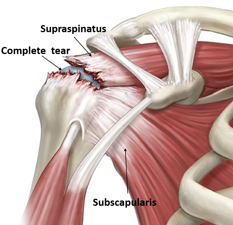
Figure 1: Shoulder anatomy [5]

Medical imaging plays a critical role in defining the extent of RCTs, which has important implications in clinical decision making and surgical planning [9]. Magnetic resonance imaging (MRI), magnetic resonance angiography (MRA) and ultrasound (US) are standard imaging modalities being used to assess the presence and size of RCTs [10]. However, these diagnostics techniques are not always accurate in depicting the size and number of involved tendons [11]. MRI as the first-choice imaging modality for the detection of RCTs is costly, bulky and is not suitable for on-site early detection. There is frequent intra-operative reports claiming to find tears much larger than determined on MRI, or even the lack of a tear [12]. MRA is an invasive procedure that requires the injection of a contrast agent [13]. US is operator-dependent and may be limited by the patients body habitus [14]. As a result, an alternative low-cost, portable and non-invasive method is demanding, specially on-site for competitive athletes such as swimmers [15]. Electromagnetic imaging (EMI) systems have shown promising results in various medical applications [16, 17, 18, 19]. Fully circular tomographic-based EMI systems are designed for different applications, such as brain [20, 21], breast  [22] and knee imaging [23]. Circular data acquisition effectively helps in increasing the cross-range resolution of the reconstructed images [24].
To the best of our knowledge, there is no EMI system to detect shoulder injuries. Designing an EMI system for the shoulder is challenging due to following reasons. Firstly, the complex anatomy of the shoulder prevents designing a fully circular phased array for spherical scan and full data acquisition. As a consequence, the antenna array has to be defined conformal to the shoulder geometry. Another challenge would be the electrically large size of the shoulder along with the heterogeneous nature of the tissues, characterized by high losses (also a characteristic of the matching medium), making it difficult to achieve a high resolution three-dimensional (3D) reconstruction. Shoulder being located in the near-field of the antenna array, an efficient 3D EM-modelling is required to consider coupling effects and near-field interactions between the imaging system and the shoulder. Besides, the variability in the shoulder anatomy among individuals prevents us to consider a particular shoulder structure as a priori knowledge. Finally, the accurate knowledge of the dielectric properties of the shoulder tissues, and more specifically the synovial fluid, remains a challenge. At the early stage design, when assessing the potential of EMI on a new application, using numerical modeling to help design the system presents several advantages: it allows to accurately model the human body complexity and electrical properties, and to simulate various anatomical scenarios in a flexible way, while reducing cost and time. In this paper, we propose a feasibility study based on numerical assessments to design a shoulder injury detection system and demonstrate its performance. We make use of an anthropomorphic numerical model of the shoulder and a built-in EM modeling based on the open source code FreeFEM, which offers flexibility in dealing with complex geometries and electrically large structures. The paper is organized as follows: Section 2 discusses the dielectric properties of the shoulder tissues, while Section 3 describes the choices for a first shoulder imaging system with a dense array of antennas to achieve high resolution. The mathematical framework of the EM modeling is outlined in Section 4, and numerical solutions are presented in Section 5. Section 6 investigates the reduction of the number of antennas in the EMI system.

2 Dielectric properties of the shoulder tissues

Once the RTCs occurs, synovial fluid (SF) accumulates at the location of the tear [25, 26] that leads to a change in the dielectric properties in the shoulder joint [27]. It is reported that the volume of SF on aspiration prior to arthroscopic rotator cuff repair correlates with tear size. The mean aspirate volume of partial tears is $0.76\pm 0.43\leavevmode\nobreak\ mL$, small tears $1.46\pm 1.88\leavevmode\nobreak\ mL\leavevmode\nobreak\$, medium tears $3.04\leavevmode\nobreak\ \pm 2.21mL\leavevmode\nobreak\$, and large tears $6.60\leavevmode\nobreak\ \pm 3.23\leavevmode\nobreak\ mL$ [26]. When there is a difference in the dielectric properties between different shoulder tissues and the SF, microwave imaging can detect this contrast. The larger the difference, the easier the detection. Thus, it is essential to measure the dielectric properties of the SF in relation to the other tissues. In a recent work with the purpose of detecting knee injury [23], high values of SF are considered compared to the rest of the tissues; however, to the best of our knowledge, no measurement of dielectric properties of SF is published in this or any other literature. It is reported that low frequencies ranging between $0.5-3\leavevmode\nobreak\ GHz$ are suitable to achieve deeper tissue penetration as well as acceptable imaging quality [28]. In this section, the dielectric properties of SF, muscle, bone cortical and tendons are measured in the frequency range of $1-4\leavevmode\nobreak\ GHz$ that almost include and extend the recommended frequency range. In the case of SF, four patients with knee or shoulder pain were sampled to obtain the real human SF. We computed the average value of the measured dielectric properties of the four SF samples, which had different temperature and pathology. The mixtures of the other tissues were made based on the SUPELEC RECIPES website [29]. An optimization code based on Kraszweski’s binary law gives the concentration of TritonX-100 and salt required to produce mixtures, whose dielectric properties are close to those given by a Cole-Cole model, for each biological tissue of the shoulder region [30]. Measurements were performed using a homemade coaxial probe connected to a ZVH8 Vector Network Analyzer [31]. Fig. 2 gathers all measurements and comparisons with values from reference websites ,. Our approach is validated by the good agreement with the references.

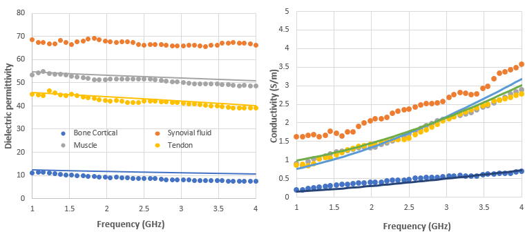
Figure 2: Dielectric properties of the tissues

The relative contrast between SF and other tissues over the frequency range of interest is around 30%, except for the muscle for which there is a 20% difference in the real part, making the tear detection feasible but challenging. The anthropomorphic shoulder model is shown in Figure 3. The complex permittivity values of the shoulder tissues at $1\leavevmode\nobreak\ GHz$ are given in Table 1 and are used in the simulations. In this Table, the SF value corresponds to our measurements, but the values of other tissues have been already available and are taken from reference websites${}^{1},^{2}$. The complex permittivity of the matching medium is chosen equal to that of the muscle.

Region	Complex Permittivity	Color in Fig. 3
Bone cortical	$12.4-2.79j$	Blue
Tendon	$45.6-13.66j$	Yellow
Muscle	$54.8-17.43j$	Transparent
Skin	$40.9-16.17j$	Green
SF	$68.0-29.0j$	Red

Table 1: Complex dielectric properties at $1\leavevmode\nobreak\ GHz$

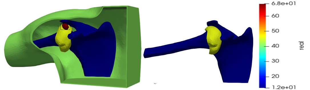
Figure 3: Shoulder Phantoms, real permittivity values

3 Electromagnetic imaging System

We first design an EMI system with a dense array of antennas that illuminates the shoulder from different angles. This multi-perspective approach helps in reconstructing a comprehensive and accurate representation of the internal structures [32]. Results will be used as reference for the optimized system described in section 6. The EMI system consists of 96 ceramic ($\varepsilon_{r}=59$) loaded open-ended waveguides arranged on $2$ metallic fully-circular and $2$ metallic half-circular layers. The two sides of the imaging chamber are open. This wearable imaging system with open sides is adapted to the real shoulder structure and designed to surround it partially, as shown in Figure 4. The width and height of the rectangular waveguides are $2.1\leavevmode\nobreak\ cm$ and $0.075\leavevmode\nobreak\ cm$, respectively. Their frequency bandwidth is $0.93-1.85\leavevmode\nobreak\ GHz$. Here, the operating frequency of $1GHz$ is chosen as a good compromise regarding penetration depth and low specific absorption rate (SAR) [33].

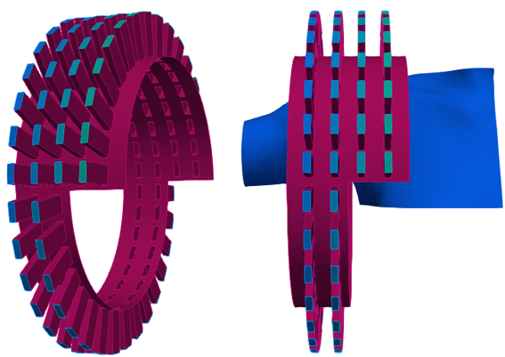
Figure 4: EMI system for the shoulder

Considering the matching medium as the reference permittivity, the wavelength in this medium is $\lambda=4.2\leavevmode\nobreak\ cm$. The diameter of the chamber is $7.14\lambda$, the larger length is $3\lambda$ and the distance between antenna layers is $0.47\lambda$. The larger size of the modeled large and partial tears is $0.69\lambda$ and $0.397\lambda$, respectively. Note that we can expect a better resolution than $0.25\lambda$, because EMI system is operating in the near field [34]. The space between antennas and the shoulder is filled with a matching medium to overcome air-skin reflections [35].

4 Mathematical Framework

4.1 Finite Element Mesh Generation

Finite element 3D mesh generation of the complete system is a challenging step due to both the complex geometry of the real body from Computer-Aided Design (CAD) models and the imaging system components. We have chosen to use realistic surface CAD models for shoulder profile and bones including humerus and scapula from a library of 3D models related to the anatomy [36]. A simple model of rotator cuff tendons was then built surrounding the shoulder joint. The skin is considered with a thickness of $2\leavevmode\nobreak\ mm$ surrounding the muscle geometry. The injury is modeled as an ellipsoid in the approximate location of the tear in the supraspinatus tendon, with two different size configurations: small tear with volume of $1mL$, and large tear with volume of $5mL$. Note that in the healthy case, the ellipsoid is replaced with muscle. The regions corresponding to the different tissues are visible in Figure 3. The remaining area (excluding bone, injury, tendon, skin) corresponds to muscle. The conformal 3D mesh of the complete system must satisfy non-overlapping elements and nodal-match conditions. At the interfaces between domains, special attention should be given to ensure that the mesh is well-aligned, conformal and continuous [37]. Taking into account that the surface meshes of some tissues intersect the imaging system boundaries, the mesh generation procedure is done by extracting and rebuilding boundary curves corresponding to each intersection for all intersecting surfaces, see Figure 5. In this work, we use the open-source finite element software FreeFEM, which allows to generate 3D meshes and solve partial differential equations (PDEs) with the finite element method (FEM) [38]. FreeFEM is interfaced with the MMG remeshing library [39, 40], which makes it possible to generate adapted tetrahedral meshes of complex geometric configurations, such as the one considered in this paper.

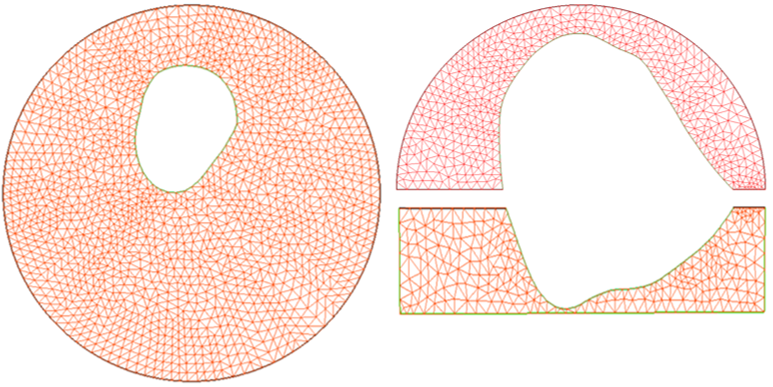
Figure 5: The intersecting surfaces of EMI system with shoulder

4.2 Forward Modeling

The 3D domain ($\Omega$) includes the imaging system and the shoulder as a heterogeneous dissipative non-magnetic medium of complex permittivity $\varepsilon_{r}=(\varepsilon_{r}^{{}^{\prime}}-\frac{\sigma j}{\omega\varepsilon_{0}})$, with $\sigma$ the conductivity and $\varepsilon_{r}^{{}^{\prime}}$ the electrical permittivity of each tissue, $\varepsilon_{0}$ the electrical permittivity of free space, and $\omega$ the angular frequency. In the frequency domain, the electric field $\xi(\mathbf{x},\mathbf{t})=\Re(\mathbf{E(x)}e^{\mathrm{i}\omega\mathbf{t}})$ has harmonic dependence on time of angular frequency $\omega$, where $\mathbf{E(x)}$ is its complex amplitude depending on the space variable $\mathbf{x}$. The boundary value problem is defined in equation 1.

$$\begin{cases}\nabla\times(\nabla\times\mathbf{E})-k^{2}\mathbf{E}=0,&\text{in }\Omega,\\ \mathbf{E}\times\textbf{n}=0,&\text{on }\Gamma_{m}\\ \nabla\times\mathbf{E}\times\textbf{n}+\mathrm{i}\beta\textbf{n}\times(\mathbf{E}\times\textbf{n})=g&\text{on }\Gamma_{t}\\ \nabla\times\mathbf{E}\times\textbf{n}+\mathrm{i}\beta\textbf{n}\times(\mathbf{E}\times\textbf{n})=0&\text{on }\Gamma_{r}\\ \nabla\times\mathbf{E}\times\textbf{n}+\mathrm{i}k\textbf{n}\times(\mathbf{E}\times\textbf{n})=0&\text{on }\Gamma_{o},\end{cases}$$ (1)

where $\mathbf{E(x)}$ is the solution of equation (1) for each transmitting antenna and $k=\omega\sqrt{\varepsilon_{r}\varepsilon_{0}\mu_{0}}$ is the complex wavenumber of the inhomogeneous medium at each point of the 3D space, with $\mu_{0}$ the permeability of free space. $\beta$ is the propagation wavenumber along the waveguide which corresponds to the propagation of the dominant transverse electric mode $TE_{10}$. The excitation term is defined as $g=2\mathrm{i}\beta\mathbf{E}^{TE_{10}}$, imposing an incident wave corresponding to the excitation of the dominant mode of the transmitting waveguide. $\Gamma_{t}$ is the port of the transmitting waveguide, $\Gamma_{r}$ corresponds to ports of receiving waveguides, $\Gamma_{m}$ represents the metallic surfaces of the waveguides and the walls between them, and $\Gamma_{o}$ represent the three open sides (right, left and bottom) of the chamber and the boundaries of shoulder profile. Let us consider $V=\{\mathbf{v}\leavevmode\nobreak\ \in\leavevmode\nobreak\ H(\mbox{curl},\Omega),\leavevmode\nobreak\ \mathbf{v}\times\mathbf{n}=0\leavevmode\nobreak\ \text{on}\leavevmode\nobreak\ \Gamma_{m}\}$, where $H(\mbox{curl},\Omega)$ is the space of square integrable functions whose curl is also square integrable, and $v$ is the test function. The variational formulation of equation (1) is: find $\mathbf{E}\leavevmode\nobreak\ \in\leavevmode\nobreak\ V$ such that:

$$\int_{\Omega}[(\nabla\times\mathbf{E})\cdot(\nabla\times\mathbf{v})-k^{2}\mathbf{E}\cdot\mathbf{v}]+\leavevmode\nobreak$$ (2)

$$\int_{\Gamma_{t}\cup\Gamma_{r}}\mathrm{i}\beta(\mathbf{E}\times\mathbf{n})\cdot(\mathbf{v}\times\mathbf{n})+\leavevmode\nobreak$$

$$\int_{\Gamma_{o}}\mathrm{i}k(\mathbf{E}\times\mathbf{n})\cdot(\mathbf{v}\times\mathbf{n}) \leavevmode\nobreak\ =\int_{\Gamma_{t}}g\cdot\mathbf{v},\leavevmode\nobreak\ \forall\leavevmode\nobreak\ \mathbf{v}\leavevmode\nobreak\ \epsilon\leavevmode\nobreak\ V.$$

Through the successive solution of variational problem (2) for each transmitting antenna, we can compute the scattering matrix, a set of complex-valued reflection and transmission coefficients, given in equation (3):

$$S_{ij}=\frac{\int_{\Gamma_{r}}\mathbf{E}\cdot\mathbf{E}^{TE_{10}}}{\int_{\Gamma_{r}}|{\mathbf{E}^{TE_{10}}}|^{2}}.$$ (3)

The computed scattering parameters form a complex matrix of size $96\times 96$, which is used to produce synthetic data by adding noise to the real and imaginary parts of the coefficients, using a multiplicative white Gaussian noise. The Gaussian noise is applied independently to the real and imaginary parts of each $S_{ij}$ coefficient as independent random variables drawn from the standard normal distribution $N(0,1)$. In this work, we have corrupted the data $S_{ij}$ with $23\leavevmode\nobreak\ dB$ noise.

4.3 Domain decomposition

The finite element discretization of our problem leads to a large ill-conditioned linear system $A\mathbf{u}=\mathbf{b}$ for each transmitting antenna. Domain decomposition methods (DDMs) are efficient tools to solve such large systems in parallel, both in terms of convergence and computing time [39]. These approaches rely on the partition of the computational domain into smaller subdomains, leading to subproblems of smaller size which are manageable by direct solvers [40]. A Krylov iterative solver (GMRES) along with an Optimized Restricted Additive Schwarz (ORAS) preconditioner is chosen to solve our problem. The domain decomposition preconditioner is implemented in the HPDDM library [41], an open source high-performance unified framework for domain decomposition methods which is interfaced with the FreeFEM software.

4.4 Inverse Problem

Let $\kappa=k^{2}$ be the unknown complex parameter of the inverse problem in each point of $\Omega$. In this step an optimization problem, including a fit-to-data term and a regularizing term, is defined with the following cost function:

$$J{(\kappa)}=\frac{1}{2}\sum_{j=1}^{N}\sum_{i=1}^{N}\frac{|S_{ij}(\kappa)-S_{ij}^{syn}|^{2}}{|S_{ij}^{empty}|^{2}}+\alpha R(\kappa).$$ (4)

Where

• $S_{ij}^{syn}$ are the scattering coefficients obtained from the forward problem and are referred to as synthetic data in the rest of the paper.

• $S_{ij}^{\kappa}$ are the scattering coefficients computed for the unknown $\kappa$ at the current iteration.

• $S_{ij}^{empty}$ are the coefficients computed from the simulation when the domain is filled only with the homogeneous matching medium, used for normalization.

• $N$ is the number of antennas of the system.

• the Tikhonov regularization method is chosen to reduce the noise effect, defined as $R(\kappa)=\frac{1}{2}\int_{\Omega}{|\nabla{\kappa}|^{2}}$.

• the regularization parameter $\alpha$ is chosen empirically equal to $10^{-6}$ to reach a good compromise between denoising as well as achieving suitable image quality with respect to certain properties such as smoothness or sparsity [42].

Minimizing functional (4) with respect to the parameter $\kappa$ is done by computing its differential and using the adjoint approach in order to simplify its expression [43]. The gradient of the resulted adjoint functional is used in the limited-memory Broyden-Fletcher-Goldfarb-Shanno (L-BFGS) optimization algorithm. We refer to [20] for a detailed description of the inverse modeling that we have followed in this work. Note that we avoid inverse crime by adding noise to the synthetic data (explained in Section 4.2) and not using a priori knowledge of the body structure. Eliminating a priori knowledge is done by using a mesh that includes the geometry and structure of the body for generating synthetic data (Figure 6, left) but defining a different homogeneous mesh that is limited to the imaging chamber (Figure 6, right) for the inverse problem. Using Nedelec edge finite elements (FE) of first polynomial degree ($r=1$) for the FE discretization results in 510531 unknowns for the direct mesh and $357535$ unknowns for the inverse mesh. The spatial resolution for both generated meshes can be defined as the number of points per wavelength $n_{\lambda}$. Here we choose $n_{\lambda}=\frac{\lambda}{6}$, where $\lambda$ corresponds to the wave propagation in the matching medium/muscle tissue.

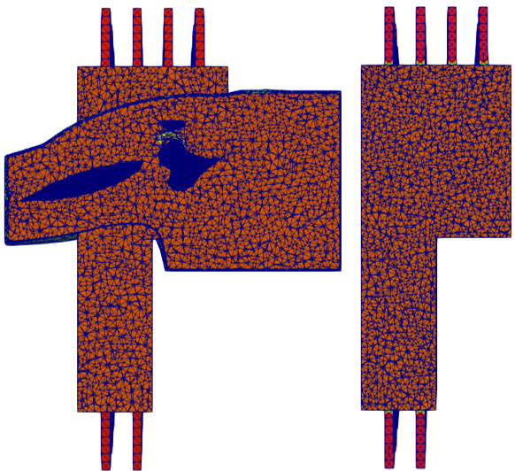
Figure 6: Left: Synthetic data, Right: Inverse problem.

5 Numerical Results

Results are obtained on the Université Côte d’Azur’s High-Performance Computing (HPC) center. In this HPC center, cluster is composed of 48 CPU computing nodes, including 32 nodes with Dual Intel Xeon Gold processor, providing 40 cores per node and 192 GB of memory and 16 nodes with 2 AMD Epyc processors, providing 32 cores per node and 256 GB of memory. The simulations presented in this paper were carried out using $480$ cores. Each reconstruction starts from an initial guess of homogeneous matching medium. The reconstruction results shown here are obtained after 60 iterations; the residual is decreased by a factor of $10^{-2}$. Subsequent iterations do not provide any further noteworthy decrease. Figures 7 and 8 show the 3D view of the exact (top) and reconstructed (bottom) results for healthy, partially and fully injured shoulder on the regions of interest. Note that in the healthy shoulder case, the ellipsoid is filled in with muscle as shown in Figs 7,  8 for comparison purpose. The rest of the muscle is not shown for the sake of visibility. The tear is visible in reconstructed real and imaginary parts. For a better view, we also plot the difference between reconstructed permittivity of healthy case and those for the partially and largely injured cases, known as differential images [44]. They are shown for the real part in Figure 9, proving that the inverse algorithm succeeds in detecting the injury, with respect to size and location, even for the partial tear. Results for the imaginary part are similar, but are not presented here for the sake of brevity.

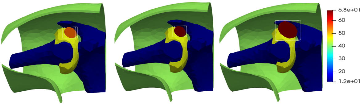
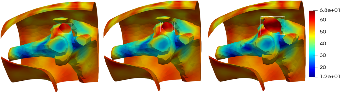
Figure 7: Cross-section of the real part of the permittivity. Top: exact permittivity, bottom: reconstructed permittivity. From left to right: Healthy, partial tear and large tear.

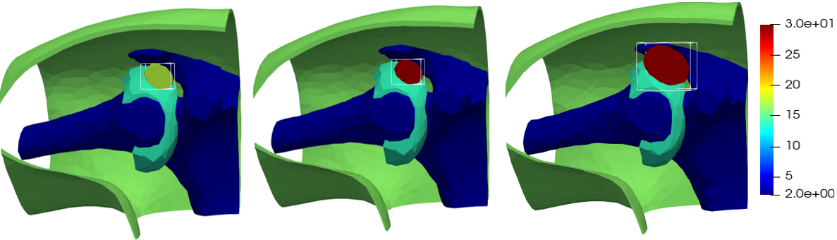
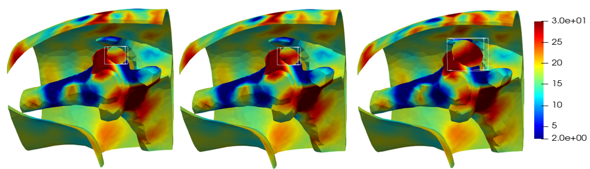
Figure 8: Cross-section of the imaginary part of the permittivity. Top: exact permittivity, bottom: reconstructed permittivity. From left to right: Healthy, partial tear and large tear.

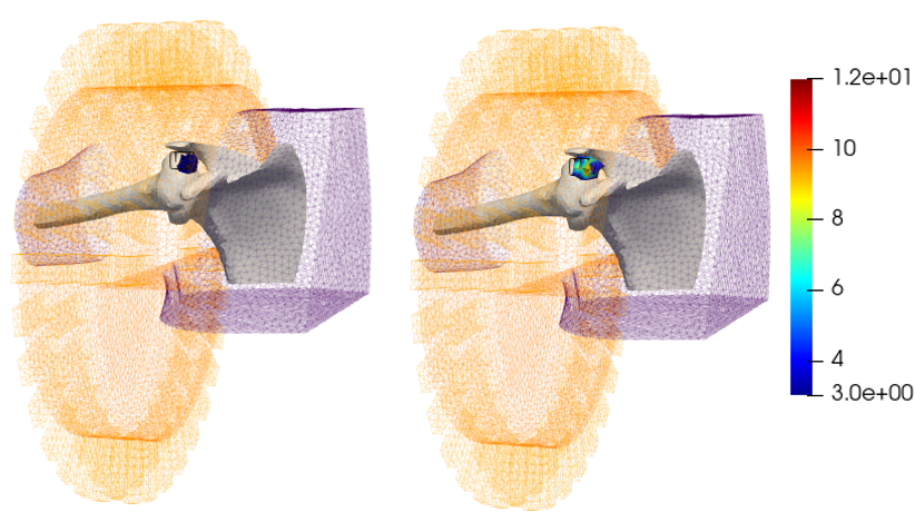
Figure 9: The differential image for partial and large tear.

$$err_{absolute}=|{\varepsilon_{r}^{reconstructed}-\varepsilon_{r}^{exact}}|$$ (5)

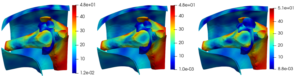
Figure 10: The absolute error on real part, from left to right: Healthy shoulder, partial and large tear

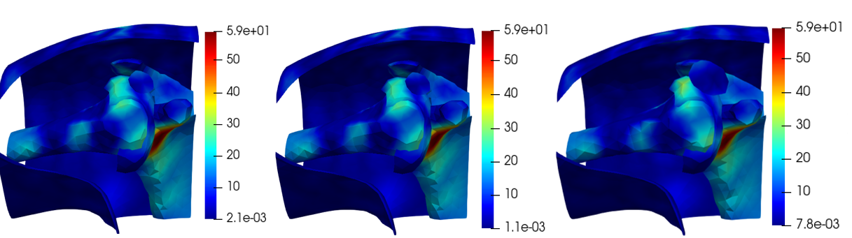
Figure 11: The absolute error on imaginary part, from left to right: Healthy shoulder, partial and large tear

The reconstruction is further assessed by computing the absolute error on the real and imaginary parts according to equation (5) applied on each pixel of the reconstructed domain. Results are shown in Figure 10 and 11. Error distribution is not uniform across tissues. Highest values are on the edges of the bone area, due to the higher contrast between the complex permittivity of bone and muscle. However, inside the bone in the areas that are not in the vicinity of the edges, the error decreases as expected, due to better performance of the inversion algorithm in a homogeneous region compared to the interfaces. The minimum values of the absolute error in the injury area are $0.78$ and $0.435$, respectively for the real and imaginary parts of the partial tear. These values for the large tear are $0.0088$ and $0.065$, respectively.

6 An improved design of EMI system

In this section, an efficient design of the imaging system in terms of reduced number of antennas is proposed. With less transmitting and receiving waveguides, faster computing time as well as cost-effective design can be achieved. The system is optimized according to the following guidelines:

• The number of antennas is a power of two to ease practically feeding signals into a switching matrix.

• We introduce a spatial shift between antennas of adjacents rings as shown in Fig. 12, in order to preserve the spatial diversity.

Different design configurations are assessed based on the value of the $L^{2}$ norm error, referred to as $err$ according to equation (6), as well as the mean value of the subtraction between the reconstructed injured model and reconstructed healthy model in the injury area, defined in equation (7). Three different configurations are considered, with 16, 32, and 64 antennas ; the reference configuration corresponds to the complete system with $96$ antennas. The values of $err$ for each configuration are computed in the whole domain as well as in the injury area for the partially injured model and are gathered in Table 2. Looking at the $err$ values on both real and imaginary parts, there is no significant increase when reducing the number of antennas by 64 ($N=32$). However, further removing $16$ antennas and going from $N=32$ to $N=16$ antennas leads to a higher increase in $err$. The trend is confirmed by looking at the contrast values $ctr$ which are shown in Table 3 for both partial and large tear and with different levels of noise. In the partial tear case, the value of $ctr$ remains positive notable for $N=32$ for all noise levels, and we expect to be able to detect the injury. In contrast, $ctr$ is either negligible or negative for $N=16$, resulting in poor differential images. A first conclusion is that the best design compromise appears to be the $N=32$ configuration, which still allows detection in the most difficult partial tear case. This was further confirmed by extracting and comparing the differential images for each configuration, but due to space limitation the images are not shown in the paper. The optimal $N=32$ antennas configuration is depicted in Figure 12 and has $11$ and $10$ antennas in both full layers and $6$ and $5$ antennas on both half layers, from left to right. Note that the computing time decreases to about half of the required time for the full $N=96$ configuration.

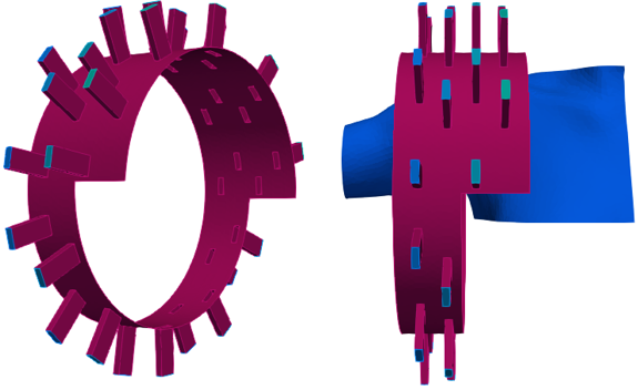
Figure 12: Optimal shoulder EMI system

$$err=\frac{||\Re(\varepsilon_{r}^{reconstructed})-\Re(\varepsilon_{r}^{exact})||_{2}}{||\Re(\varepsilon_{r}^{exact})||_{2}}$$ (6)

$$ctr=\varepsilon_{r}^{injured}-\varepsilon_{r}^{healthy}$$ (7)

Table 2: $err$ in the injury area and total domain for the partial tear case, and computing time.

N	Total		Injury		time
	real	imaginary	real	imaginary	(min:s)
96	$8.8\%$	$21.4\%$	$14\%$	$24.4\%$	$20:09$
64	$9.0\%$	$21.2\%$	$10.4\%$	$19.2\%$	$16:24$
32	$9.4\%$	$20.6\%$	$16.8\%$	$33.3\%$	$12:02$
16	$10.8\%$	$17.2\%$	$19.3\%$	$45.9\%$	$11:27$

Table 3: $ctr$ in the injury area for partial and large tears with different noise levels.

	N	Noise of 23 dB		Noise of 15 dB		Noise of 10 dB
		real	imaginary	real	imaginary	real	imaginary
Partial	96	$1.803$	$1.910$	$1.934$	$1.767$	$1.973$	$1.696$
	64	$1.605$	$1.673$	$1.664$	$1.654$	$2.233$	$1.503$
	32	$0.890$	$0.690$	$0.843$	$0.669$	$0.599$	$0.681$
	16	$0.133$	$0.1918$	$-0.136$	$0.0193$	$0.3617$	$0.256$
Large	$96$	$5.254$	$5.101$	$5.182$	$5.230$	$5.412$	$5.033$
	$64$	$5.053$	$4.312$	$5.145$	$4.310$	$5.396$	$4.244$
	$32$	$2.322$	$2.241$	$2.467$	$2.191$	$2.524$	$2.204$
	$16$	$0.750$	$0.711$	$0.692$	$0.681$	$0.787$	$0.780$

7 Conclusion

We have conducted the first numerical study on the feasibility to image the shoulder joint with an EMI system. The first part of the study consisted in the investigation of the dielectric properties of the shoulder tissues, in particular the synovial fluid which was measured for the first time. Secondly, we have shown that it is possible to reconstruct 3D images of the shoulder joint based on an anthropomorphic numerical model of the shoulder with an imaging system composed of a dense array of $96$ antennas. The reconstruction takes $20$ minutes and $9$ seconds on $480$ computing cores and shows great promise for rapid diagnosis or medical monitoring. Finally, we take advantage of numerical modeling to optimize the number of antennas in the EMI system. We achieve a drastic reduction from $96$ to $32$ antennas. After having proved the relevance of microwave imaging for the detection of shoulder injury, the next step will be to manufacture the imaging system and conduct measurements on built-in phantoms of the different tissues in order to further validate the imaging system proposed in this work.

References

- [1] Barbara Juliette Mera “Current perspectives on rotator cuff disease” In Osteology 2.2 MDPI, 2022, pp. 62–69
- [2] Richard W Nyffeler, Nicholas Schenk and Philipp Bissig “Can a simple fall cause a rotator cuff tear? Literature review and biomechanical considerations” In International orthopaedics 45 Springer, 2021, pp. 1573–1582
- [3] Jeffrey R Dugas et al. “Anatomy and dimensions of rotator cuff insertions” In Journal of shoulder and elbow surgery 11.5 Elsevier, 2002, pp. 498–503
- [4] Reza Omid and Brian Lee “Tendon transfers for irreparable rotator cuff tears” In JAAOS-Journal of the American Academy of Orthopaedic Surgeons 21.8 LWW, 2013, pp. 492–501
- [5] Dr. Fernando Cinagava “https://consultoriodoombro.com.br/por-que-meus-ombros-doem-com-video-explicativo-sobre-tendinite-do-ombro/”
- [6] Umile Giuseppe Longo et al. “Histopathology of rotator cuff tears” In Sports Medicine and Arthroscopy Review 19.3 LWW, 2011, pp. 227–236
- [7] Atsushi Yamamoto et al. “The impact of faulty posture on rotator cuff tears with and without symptoms” In Journal of shoulder and elbow surgery 24.3 Elsevier, 2015, pp. 446–452
- [8] Ali Abdelwahab et al. “Traumatic rotator cuff tears-Current concepts in diagnosis and management” In Journal of Clinical Orthopaedics and Trauma 18 Elsevier, 2021, pp. 51–55
- [9] Gabrielle P Konin “Imaging of the Rotator Cuff” In Massive Rotator Cuff Tears: Diagnosis and Management Springer, 2014, pp. 31–51
- [10] Joseph P Iannotti et al. “Accuracy of office-based ultrasonography of the shoulder for the diagnosis of rotator cuff tears” In JBJS 87.6 LWW, 2005, pp. 1305–1311
- [11] Sharlene A Teefey et al. “Detection and quantification of rotator cuff tears: comparison of ultrasonographic, magnetic resonance imaging, and arthroscopic findings in seventy-one consecutive cases” In JBJS 86.4 LWW, 2004, pp. 708–716
- [12] Xusheng Li et al. “The accuracy of MRI in diagnosing and classifying acute traumatic multiple ligament knee injuries” In BMC Musculoskeletal Disorders 23 Springer, 2022, pp. 1–7
- [13] Ashley Yip et al. “Magnetic resonance imaging compared to ultrasonography in giant cell arteritis: a cross-sectional study” In Arthritis research & therapy 22.1 BioMed Central, 2020, pp. 1–8
- [14] Mark Adrian “MRI: understanding its limitations” In Br Columb Med J 47, 2005, pp. 359–361
- [15] JT Stahnke, M Schenk and KP Sharpe “Magnetic Resonance Imaging of Symptomatic Swimmer’s Shoulder” In Int J Radiol Imaging Technol 6, 2020, pp. 070
- [16] Kazuki Kanazawa, Kazuki Noritake, Yuriko Takaishi and Shouhei Kidera “Microwave imaging algorithm based on waveform reconstruction for microwave ablation treatment” In IEEE Transactions on Antennas and Propagation 68.7 IEEE, 2020, pp. 5613–5625
- [17] Daniel Oloumi et al. “Microwave imaging of breast tumor using time-domain UWB circular-SAR technique” In IEEE Transactions on Medical Imaging 39.4 IEEE, 2019, pp. 934–943
- [18] Amir Mirbeik-Sabzevari et al. “Synthetic ultra-high-resolution millimeter-wave imaging for skin cancer detection” In IEEE Transactions on Biomedical Engineering 66.1 IEEE, 2018, pp. 61–71
- [19] Kamel S Sultan, Beadaa Mohammed, Mohamed Manoufali and Amin M Abbosh “Portable electromagnetic knee imaging system” In IEEE Transactions on Antennas and Propagation 69.10 IEEE, 2021, pp. 6824–6837
- [20] Pierre-Henri Tournier et al. “Numerical modeling and high-speed parallel computing: New perspectives on tomographic microwave imaging for brain stroke detection and monitoring” In IEEE Antennas and Propagation Magazine 59.5 IEEE, 2017, pp. 98–110
- [21] Markus Hopfer et al. “Electromagnetic Tomography for Detection, Differentiation, and Monitoring of Brain Stroke: A Virtual Data and Human Head Phantom Study.” In IEEE Antennas and Propagation Magazine 59.5 IEEE, 2017, pp. 86–97
- [22] Caroline Zellweger et al. “Breast computed tomography: diagnostic performance of the maximum intensity projection reformations as a stand-alone method for the detection and characterization of breast findings” In Investigative Radiology 57.4 Wolters Kluwer, 2022, pp. 205–211
- [23] Kamel Sultan “Design and implementation of electromagnetic knee imaging systems”, 2022
- [24] Lulu Wang “Microwave Imaging and Sensing Techniques for Breast Cancer Detection” In Micromachines 14.7 MDPI, 2023, pp. 1462
- [25] Athanasios Papatheodorou et al. “US of the shoulder: rotator cuff and non–rotator cuff disorders” In Radiographics 26.1 Radiological Society of North America, 2006, pp. e23–e23
- [26] Michael Stone et al. “Synovial fluid volume at the time of arthroscopic rotator cuff repair correlates with tear size” In Cureus 12.7 Cureus, 2020
- [27] John Kiel and Eamon Olwell “It might be a tumor: a unique presentation of a chronic rotator cuff tear” In African Journal of Emergency Medicine 10.4 Elsevier, 2020, pp. 288–290
- [28] Natalia K Nikolova “Microwave imaging for breast cancer” In IEEE microwave magazine 12.7 IEEE, 2011, pp. 78–94
- [29] “SUPELEC RECIPES, Standard Uwb Phantom ELECtromagnetic Recipes [online]. Available http://applis.iut.univ-paris-diderot.fr/CNRS/.”
- [30] Sami Gabriel, RW Lau and Camelia Gabriel “The dielectric properties of biological tissues: III. Parametric models for the dielectric spectrum of tissues” In Physics in medicine & biology 41.11 IOP Publishing, 1996, pp. 2271
- [31] Soroush Abedi, Hélène Roussel and Nadine Joachimowicz “Standardized Phantoms” In Electromagnetic Imaging for a Novel Generation of Medical Devices: Fundamental Issues, Methodological Challenges and Practical Implementation Springer, 2023, pp. 1–32
- [32] Chang Liu et al. “Multi-perspective ultrasound imaging technology of the breast with cylindrical motion of linear arrays” In Applied Sciences 9.3 MDPI, 2019, pp. 419
- [33] Kamel S Sultan, Ahmed Mahmoud and Amin M Abbosh “Textile electromagnetic brace for knee imaging” In IEEE Transactions on Biomedical Circuits and Systems 15.3 IEEE, 2021, pp. 522–536
- [34] Tie Jun Cui, Weng Cho Chew, Xiao Xing Yin and Wei Hong “Study of resolution and super resolution in electromagnetic imaging for half-space problems” In IEEE Transactions on Antennas and Propagation 52.6 IEEE, 2004, pp. 1398–1411
- [35] Hoi-Shun Lui, Andreas Fhager and Mikael Persson “Matching medium for biomedical microwave imaging” In 2015 International Symposium on Antennas and Propagation (ISAP), 2015, pp. 1–3 IEEE
- [36] “Plasticboy, Blender Rigged V07 Anatomy 3D models store [online]. Available https://www.plasticboy.co.uk/store/index.html”
- [37] Richard Michael Jack Kramer and David R Noble “Guaranteed Quality Conformal Mesh Decomposition.”, 2015
- [38] Frédéric Hecht “New development in FreeFem++” In Journal of numerical mathematics 20.3-4 De Gruyter, 2012, pp. 251–266
- [39] Niall Bootland, Sahar Borzooei, Victorita Dolean and Pierre-Henri Tournier “Numerical assessment of PML transmission conditions in a domain decomposition method for the Helmholtz equation” In arXiv preprint arXiv:2211.06859, 2022
- [40] Sahar Borzooei, Victorita Dolean, Pierre-Henri Tournier and Claire Migliaccio “Solution of time-harmonic Maxwell’s equations by a domain decomposition method based on PML transmission conditions” In arXiv preprint arXiv:2211.04912, 2022
- [41] Pierre Jolivet, Frédéric Hecht, Frédéric Nataf and Christophe Prud’Homme “Scalable domain decomposition preconditioners for heterogeneous elliptic problems” In Proceedings of the International Conference on High Performance Computing, Networking, Storage and Analysis, 2013, pp. 1–11
- [42] Yuhui Zheng, Min Li, Jianwei Zhang and Jin Wang “Selection of regularization parameter in GMM based image denoising method” In Multimedia Tools and Applications 77 Springer, 2018, pp. 30121–30134
- [43] P.-H. Tournier et al. “Microwave tomographic imaging of cerebrovascular accidents by using high-performance computing” In Parallel Computing 85, 2019, pp. 88–97 DOI: https://doi.org/10.1016/j.parco.2019.02.004
- [44] R Scapaticci, OM Bucci, I Catapano and L Crocco “Differential microwave imaging for brain stroke followup” In International Journal of Antennas and Propagation 2014 Hindawi, 2014