Low-order Linear Parameter Varying Approximations for Nonlinear Controller Design for Flows

Abstract

The control of nonlinear large-scale dynamical models such as the incompressible Navier-Stokes equations is a challenging task. The computational challenges in the controller design come from both the possibly large state space and the nonlinear dynamics. A general purpose approach certainly will resort to numerical linear algebra techniques which can handle large system sizes or to model order reduction. In this work we propose a two-folded model reduction approach tailored to nonlinear controller design for incompressible Navier-Stokes equations and similar PDE models that come with quadratic nonlinearities. Firstly, we approximate the nonlinear model within in the class of LPV systems with a very low dimension in the parametrization. Secondly, we reduce the system size to a moderate number of states. This way, standard robust LPV theory for nonlinear controller design becomes feasible. We illustrate the procedure and its potentials by numerical simulations.

I Introduction

We consider general nonlinear, control-affine systems of type

$$\dot{x}(t)=f(x(t))+Bu(t),$$ (1)

where $x$ is the system’s state with values in $\mathbb{R}^{n}$ with $n$ possibly large, where $u$ is the input with values in $\mathbb{R}^{p}$, and where $f\colon\mathbb{R}^{n}\to\mathbb{R}^{n}$.

The computer-aided controller design for (1) with $n$ large is a challenging problem with no generic approach being established yet. Commonly used methods like backstepping [1], feedback linearization [2, Ch. 5.3], or sliding mode control [3] require structural assumptions and, thus, may not be accessible to a general computational framework. The both holistic and general approach via the HJB equations is only feasible for very moderate system sizes or calls for model order reduction; see, e.g., [4] for a relevant discussion and an application in fluid flow control. As an alternative to reducing the systems size, one may consider approximations to the solution of the HJB of lower complexity. For that, e.g., truncated polynomial expansions [5] are considered or heuristic approximative solutions via the so called state-dependent Riccati equation; see, e.g., [6, 7].

In this work, we propose the embedding of (1) into the class of linear parameter-varying (LPV) systems of type

$$\dot{x}(t)=A(\rho(t))\,x(t)+Bu(t),$$ (2)

with $A(\rho(t))\in\mathbb{R}^{n\times n}$ for parameter values $\rho(t)\in\mathbb{R}^{r}$ by implementing two layers of complexity reduction so that established theory and algorithms ([8]) for robust LPV controller design become available.

As laid out in [9], the controller design techniques for LPV systems can be classified into the categories polytopic, LFT-based, and gridding.

A general assumption of all these approaches is that the set of possible parameter values is bounded. If, in addition, the parameter dependency of the coefficients is affine-linear, then the theory and the related computations simplify significantly; see, e.g., [8, 10].

The polytopic approach is seen as the most developed approach with the notable results from [8, 11] that provide algorithms and theory for a scheduled $H_{\infty}$-robust controller and that are the base of the hinfgs routine in the MATLAB Robust Control Toolbox.

In a first approximation step, we seek for very low-dimensional encodings of the states for replacing the nonlinear source terms by a low-dimensional linear parameter varying (LPV) surrogate. In this step that is directed to adapt the nonlinearity to a format that is accessible to the LPV theory for computer-aided controller design, we tailor the approximations for a best representation of the source terms at very low-dimensions.

We will show that this approach can lead to LPV models that well approximate the actual dynamics with as much as $r$ dimensions in the parametrization, with $r$ well less than $10$. Thus, application of standard linear matrix inequalities (LMI) approaches already comes into reach. Still, this would require the solution of at least $r+1$ but more likely of about $2^{r}$ coupled LMIs of the size of the original system. Therefore, we propose a second layer of approximation that is tailored for the low-order LPV representation to accurately follow the original dynamics with a moderately sized state space.

This integrated approach to nonlinear controller design via tailored approximations and established robust LPV theory has not been considered so far.

Direct relations to the vast research on LPV systems are given as follows. Although the typically considered LPV systems are of moderate size (see [9, Tab. V] that classifies state space dimensions larger than $10$ as high dimensional), the unfavourable increase of complexity with the parameter dimension has triggered various work on reducing the so-called scheduling dimension; see, e.g., [12], [13], [14], or [15] that base on sparse optimization, principal component analysis (PCA), auto encoders, or general deep neural networks, respectively.

The idea of using model order reduction in combination with LPV controller design has been followed by [16] where a PDE system is reduced as a whole before the treatment as an LPV system. Recently, we have delivered a proof of concept ([7]) that LPV approximations of nonlinear systems can with low parameter dimensions work well for nonlinear controller design.

II POD for low-dimensional LPV approximations

Under mild conditions (see, e.g., [17]), the system (1) can be brought into the so-called state-dependent coefficient (SDC) form

$$\dot{x}(t)=A(x(t))\,x(t)+Bu(t),$$ (3)

with $A(x(t))\in\mathbb{R}^{n\times n}$. We will assume that, in particular, the map $x\to A(x)\in\mathbb{R}^{n\times n}$ is (affine) linear, i.e. $A(x)$ can be realized as $A(x)=A_{0}+L(x)$ with $L$ linear.

Remark II.1.

For some systems like the spatially-discretized Navier-Stokes equations the SDC representation with affine dependencies is naturally induced by its structure; see [18]. If the map $x\to A(x)$ is not linear, one can seek to find an approximation that is linear; see, e.g., [15].

We note that (3) is an LPV representation (2) of (1) with the trivial parametrization $\rho(t)=x(t)$ and with, in particular, a large parameter dimension namely $r=n$.

Next we illustrate how a general model order reduction scheme, can provide LPV approximations with possibly low-dimensional, e.g., $r\ll n$, parameter domains.

Let $V_{r}\in\mathbb{R}^{n\times r}$ be a POD basis that encodes and decodes the state $x(t)$ as $\rho(x(t))=V_{r}^{T}x(t)$ and

$$x(t)\approx\tilde{x}(t)=V_{r}\rho(x(t))=\sum_{i=1}^{r}v_{i}\rho_{i}(x(t)),$$

where $v_{i}\in\mathbb{R}^{n}$ is the $i$-th POD mode.

With this encoding and decoding, the nonlinear term in system (3) can be approximated as

$$\begin{split}A(x(t))\,x(t)\approx A(\tilde{x}(t))\,x(t)=\\ A(\sum_{i=1}^{r}v_{i}\rho_{i}(t))\,x(t)=[A_{0}+\sum_{i=1}^{r}\rho_{i}(t)L(v_{i})]\,x(t)\end{split}$$

which defines an affine-linear low-dimensional LPV approximation

$$\tilde{x}(t)=[A_{0}+\sum_{i=1}^{r}\rho_{i}(\tilde{x}(t))L(v_{i})]\,\tilde{x}(t)+Bu(t)$$ (4)

to (3) and (1). We set

$$A_{i}:=L(v_{i}),\quad i=1,\dotsc,r.$$ (5)

In the second step, we now project the LPV approximation to reduced order coordinates. For that let $V_{k}$ with $k\geq r$ be the POD basis that includes $V_{r}$ and $\bar{\rho}(t)=V_{k}\tilde{x}(t)$. Then an approximation to (4) with state dimension $k$ (as opposed to $n$) reads

$$\dot{\bar{\rho}}(t)=[\bar{A}_{0}+\sum_{i=1}^{r}\bar{\rho}_{i}(t)\bar{A}_{i}]\,\bar{\rho}(t)+\bar{B}u(t).$$ (6)

with $\bar{A}_{i}:=V_{k}^{T}A_{i}V_{k}$, for $i=0,1,\dots,r$ and $\bar{B}:=V_{k}^{T}B$.

Note that $r$ can be chosen independently of $k$. Thus, a very low-dimensional approximation can be achieved independently of a possibly larger state space that can be tailored for the best compromise in terms of size and accuracy.

III Controller Design for LPV Systems

The polytopic approach is seen as the most developed approach with the notable results from [8, 11] that provide algorithms and theory for a scheduled robust controller and that are the base of the hinfgs routine in the MATLAB Robust Control Toolbox.

IV Implementation Issues

For the computation of the snapshots that are used to extract the POD basis, a forward simulation for an example input is performed.

IV-A Polytope or Bounding Box

The computed snapshots are then projected to the $\rho$-coordinates in order to estimate the polytope $W\subset\mathbb{R}^{r}$ that contains $\rho(t)$.

The vertices $w_{i}$ of $W$ are then used to define the controller.

Intuitively, the performance of the controller will be better if the volume $|W|$ of $W$ is smaller and if the vortices $w_{i}$ are closer to extremal values of $\rho(t)$. In this respect, the optimal choice of $W$ would be the convex hull of the snapshots of $\rho$.

On the other hand, the convex hull is likely to have a large number of vortices, which makes the application of LPV controller design approaches costly as they, e.g., require the solution of $n$ coupled LMIs where $n$ is the number of vertices of $W$.

Typically, $W$ is chosen as a bounding box with, accordingly, $2^{r}$ vortices. In order to reduce the volume, the box can be rotated and expressed in coordinates obtained of the principal components; see, e.g., [13]. In our affine-linear case (4) with

$$\rho(t)=U_{\mathsf{p}c}U_{\mathsf{p}c}^{T}\rho(t)=:U_{\mathsf{p}c}\rho_{\mathsf{p}c}(t)$$ (7)

and, accordingly,

$$\tilde{x}(t)=V_{r}\rho(t)=V_{r}U_{\mathsf{p}c}\rho_{\mathsf{p}c}(t)=:\sum_{i=1}^{r}v_{{\mathsf{p}c},i}\rho_{{\mathsf{p}c},i}(t)$$ (8)

where $U_{\mathsf{p}c}$ is the principal components coordinate transformation, this reparametrization reads

$$\sum_{i=1}^{r}\rho_{i}(t)A_{i}=L(\tilde{x}(t))=\sum_{i=1}^{r}\rho_{{\mathsf{p}c},i}(t)A_{{\mathsf{p}c},i},$$ (9)

where $A_{{\mathsf{p}c},i}:=L(v_{{\mathsf{p}c},i})$ and $v_{{\mathsf{p}c},i}$ denoting the $i$-th column of $V_{r}U_{\mathsf{p}c}$, for $i=1,\dotsc,r$. For a direct retransformation of the system, we can also resort to the relation

$$A_{{\mathsf{p}c},i}=\sum_{j=1}^{r}U_{ji}A_{j},$$ (10)

where $U_{ji}$ is the $j$-th row entry of the $i$-th column of $U_{\mathsf{p}c}$.

Adding on these standard ways on defining the parameter domains, in our examples we use optimization to find a suitable polytope that gives a good compromise of volume and number of vortices and that underbids the bounding box in both variables. For this, the following optimization setup was defined and solved using the built-in methods of computing convex hulls and genetic optimization in SciPy; see, e.g., [19].

• Let $V\in\mathbb{R}^{r}$ be (the set of vertices of) the convex hull of given measurements of $\rho(x(t_{j}))$, for $j=1,\dots,N$ and a given state trajectory $x$.

• In the $i$-th iteration, extend $V$ by $n_{k}$ vertices $v^{(i)}_{k}\in\mathbb{R}^{r}$ and compute the convex hull $V^{(i)}$ of $V\cup\{v^{(i)}_{1},\dotsc,v^{(i)}_{n_{k}}\}$

• Update $v^{(i)}_{k}$ to minimize both the volume and the number of vertices of $V^{(i)}$.

We report on efficiency (and feasibility) of the computation of the LPV controller and on its performance for the three approaches of considering

• the bounding box in the original $\rho(t)$ coordinates,

• the bounding box in the PCA coordinates of $\rho(t)$, or

• an optimized polytope of fewer vertices

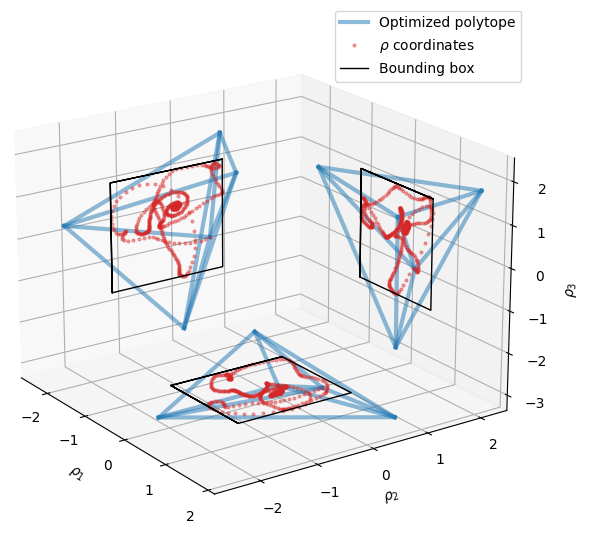
as the polytope for the parameter variation; see Figure 1 for an illustration of the bounding box and an optimized polytope.

Figure 1: An illustration of the first three components of $\rho(t)$, of the bounding box (with 8 vortices), and an optimized polytope of less volume and with only 5 vortices). Each data object is in three-dimensional space but projected along the coordinate axes to planes in the two-dimensional space.

V Numerical Example

Figure 2: Illustration of the computational domain and the developed state of the uncontrolled flow field.

We consider the two-dimensional cylinder wake with control at moderate Reynolds numbers; see Figure 2. The controls are designed as two outlets at the cylinder periphery of size $\pi/6$ located at $\pm\pi/3$ through which fluid can be injected or sucked away. Mathematically, the control is modelled by parabola-shaped spatial shaped function that is scaled by the scalar control value. For inclusion in the FEM scheme, these Dirichlet conditions are relaxed towards Robin-type boundary conditions with a relaxation parameter $\epsilon=10^{-5}$; see [20] for implementation details.

As the output $y$, we consider averaged velocities in 3 square domains of observations of size $D^{2}$ located at a distance of $H$ behind the cylinder symmetrically with respect to the channel middle. Here $D$ denotes the diameter of the cylinder and $H$ the height of the channel. With the two components of the velocity, overall, an output $y(t)\in\mathbb{R}^{6}$ is obtained with the first 3 values corresponding to the stream wise components and the final 3 values to the lateral components of the velocities.

The corresponding PDE model is spatially discretized by Taylor-Hood quadratic-linear mixed finite elements on a nonuniform grid. From the FEM model of about 50 000 degrees of freedom, the low-dimensional LPV approximation is obtained through the following algorithm

1. Starting from the steady-state solution, the FEM model is integrated in time from $t=0$ to $t=5$ with a test input applied to trigger the instabilities.

2. From the FEM solution, 417 equispaced snapshots are collected to define the POD basis.

3. With the POD basis, the reduced order LPV approximation as in (6) is computed.

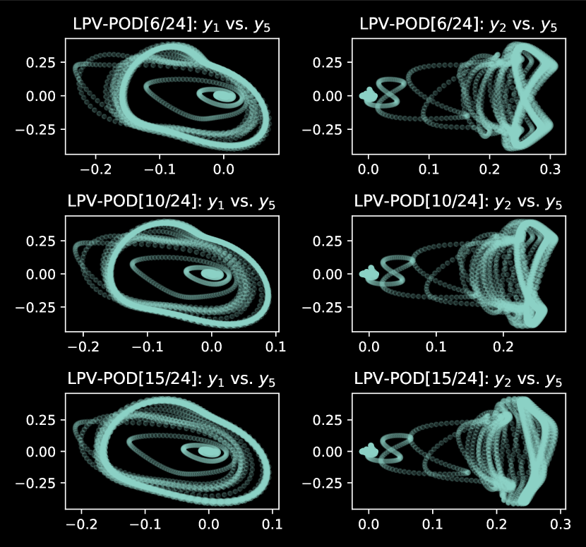
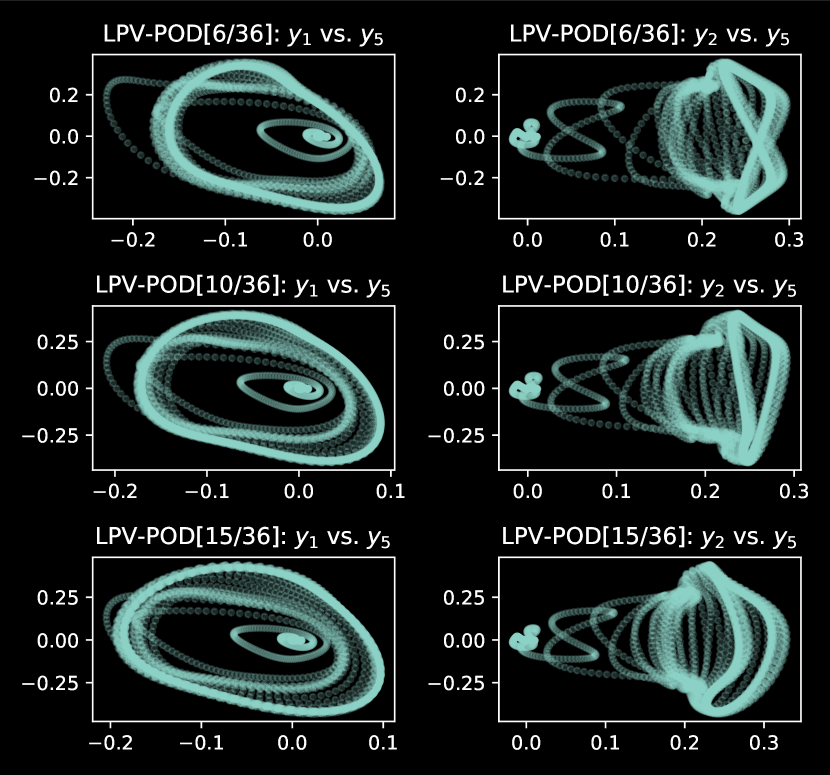
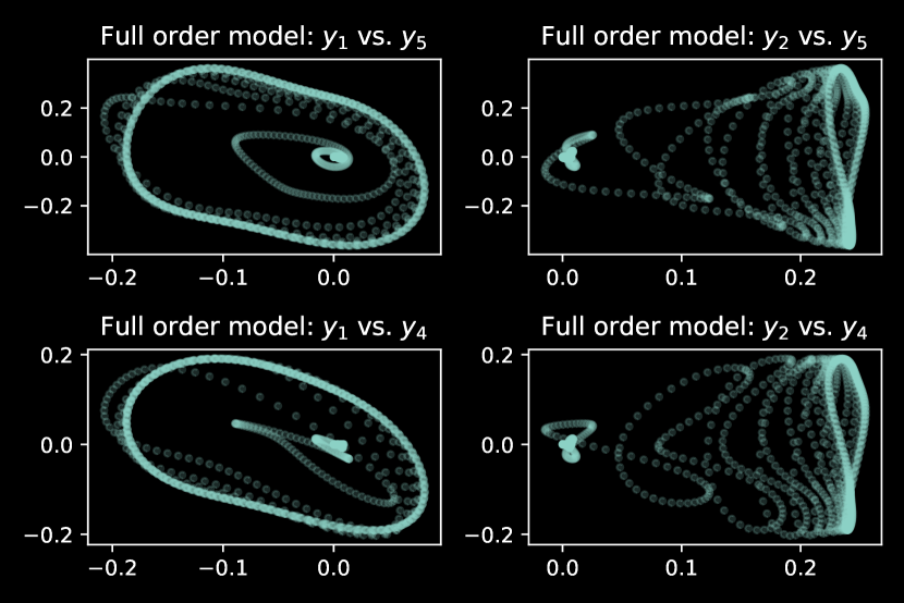
In view of determining $k$ and $r$, i.e., the size of the POD reduced model and the size of the parameter in the LPV approximation, we note that the system is chaotic which makes a quantitative decision delicate (as small perturbations have arbitrarily large effects). That’s why we took the qualitative view of examining the resulting limit cycles of selected components in the phase portraits of $y_{2}$ vs. $y_{5}$ and $y_{1}$ vs. $y_{5}$, see Figures 3–4 for results of different choices of $k$ and $r$ and Figure 5 for the reference. These phase portraits show the data points, say $(y_{2}(t_{i}),y_{5}(t_{i}))$, for $500$ time equidistant instances $t_{i}$ from the output $y$ of the corresponding simulations with zero inputs on the time interval $(0,12)$.

For the following numerical studies we chose the setup $k=36$ and $r=6$ that, judging from Figure 4 (first line) in comparison to Figure 5 (first line), seems to well cover at least the range of values in the phase portraits for the smaller values of $r$.

Figure 3: Phase portraits $y_{2}$ vs. $y_{5}$ and $y_{1}$ vs. $y_{5}$ of the output $y$ for POD dimension $k=24$ and parameter dimension $r=6,10,15$ on the time interval $(0,12)$.

Figure 4: Phase portraits $y_{2}$ vs. $y_{5}$ and $y_{1}$ vs. $y_{5}$ of the output $y$ for POD dimension $k=36$ and parameter dimension $r=6,10,15$ on the time interval $(0,12)$.

Figure 5: Phase portrait of selected components of the output $y$ for the full order FEM model on the time interval $(0,12)$. Because of the symmetry of the overall setup, the phase portraits of the remaining components bear no additional information and are not shown here.

V-A Computing the LPV Controller

For the computation of the LPV controller we used the Matlab Robust Control Toolbox[21] in the release 2022b with built-in function hinfgs that computes an LPV controller with a guaranteed quadratic robustness performance $\gamma_{*}$. The computational costs of the underlying optimization with coupled LMI constraints are significant and make larger values of $k$ and $r$ quickly infeasible for numerical studies.

As for the different approaches of defining the enclosing polytope $W\supseteq\{\rho(t)\colon t>0\}$ we made the following observations.

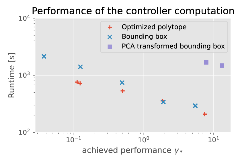
• The bounding box in the original coordinates with $2^{6}=64$ achieves the best robustness performances $\gamma_{*}$ though with rather high computational costs.

• The bounding box in the PCA coordinates comes with the same number of vertices to consider. However, the observed convergence in $\gamma_{*}$ was tediously slow which led to infeasible numerical costs for lower target values of $\gamma_{*}$.

• Using an optimized polytope of $20$ vertices, each iteration in the hinfgs computation was sped up by a factor of $3$ which well compensated for an overall slower convergence. However the slower convergence even led to stagnation so that the best achievable values of $\gamma_{*}$ were larger than that of the bounding box approach.

The results on the performance of hinfgs for the different setups and for different levels of $\gamma_{*}$ are displayed in the chart of Fig. 6. The conducted experiments suggest that a compact representation of $W$ (in the sense that its vertices are evenly distributed in space or that the ratio of surface over volume of $W$ is rather small) is beneficial for convergence in $\gamma_{*}$. Apparently, the vertices of the optimized polytope are further apart (see Fig. 1) which may explain the slower convergence and earlier stagnation. An explanation for the minor performance of the PCA coordinate transformation may call on the interpretation of the PCA concentrating the variance of the data in the leading principal components. This may result in vertices that widely distributed in one dimension and closely located in another. Nonetheless, the strong (in this case negative) effect supports the idea that a transformation of the $\rho$ coordinates has the potential of improving the performance of hinfgs.

Figure 6: Achieved $\gamma_{*}$ versus CPU time (values of three consecutive simulations) for the bounding box, the PCA transformed coordinates, and the optimized vertices setup. The left most values correspond to the best achieved $\gamma_{*}$ for which the iteration stagnates.

V-B Nonlinear Closed Loop Simulations

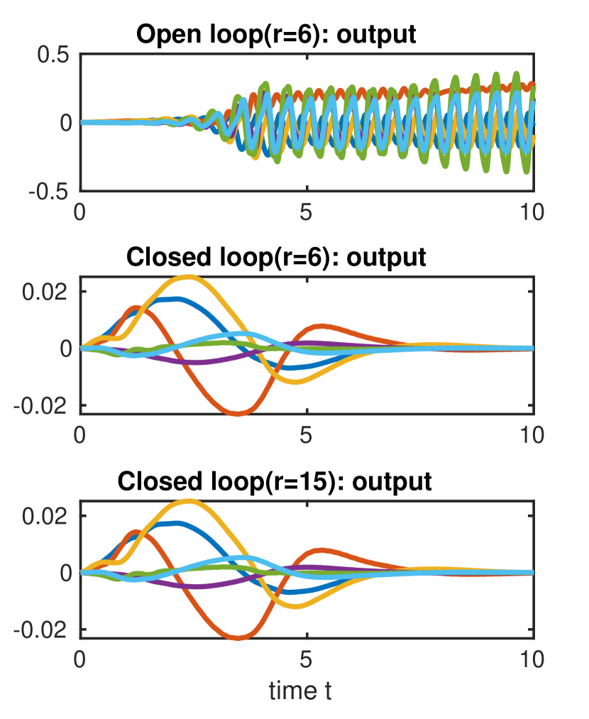
Since the robust control toolbox in Matlab does not provide the functionality to evaluate the LPV controller within a general polytope, we considered closed loop simulations with the controller obtained through the bounding box approach. Also the built-in simulation routines only support predefined parameter trajectories so that the closed-loop system was set up manually and simulated with the time integrator ode15s.

As the result, this nonlinear controller did well stabilize the nonlinear system (with $r=6$ that it was built upon) as illustrated in Fig. 7. Also, this controller proved a certain robustness by performing similarly well for the model with parameter dimension $r=15$ which is similar but also shows different dynamical patterns; cp. Fig. 4(first row vs. third row).

Figure 7: The open loop output of the model for $r=6$ and the closed loop for LPV controller designed for the $r=6$ model applied to this model and used in the larger ($r=15$) model.

V-C Remarks on Nonlinear Systems as LPV Systems

Although the embedding of a nonlinear system via $A(\rho(t))=A(\rho(x(t))$ into the class of LPV systems is readily covered by the available LPV theory, it comes with practical consequences in the controller definition. Firstly, as the trajectory of $\rho$ is not preset but defined through the state trajectory $x$, the containing polytope (or bounding box) has to be estimated from state estimations or approximations.

Secondly, the effect of the feedback is ambivalent. While a functioning controller will stabilize the system around the working point and, thus, prevent $x$ and $\rho(x)$ from attaining extreme values, short-term perturbations may lead to overshoots which can drive the system out of the estimated region.

While, practically, such an overshoot can often be compensated, the computed controller will fail immediately as the parameter update for the controller is no more well-defined. In our experiments we observed these critical overshoots when considering nonzero initial values or discontinuous disturbance signals. Therefore, in the presented simulations, we started from the zero initial conditions and applied a disturbance that smoothly faded out after $t=2$.

V-D Code Availability

The LPV system data (ready for import in Matlab) and the scripts that were used to obtain the presented numerical results are available for immediate reproduction from doi:10.5281/zenodo.10073483 under a CC-BY license.

VI Conclusions and Outlook

In this work, we have employed a two-level model order reduction approach so that, eventually, established LPV theory and algorithms become available for nonlinear controller design for general nonlinear systems like the incompressible Navier-Stokes equations.

In a numerical experiment, we illustrated the potential and feasibility of the combined approach and identified pitfalls of the approach as well as limits in the existing functionality of standard control systems software.

Notably, although the theory applies and although favourable properties of tailored polytopes have been illustrated, routines for LPV controller synthesis basically only allow for bounding boxes as enclosing polytopes. Thus, a future work will concern interpolation of controllers in polytopes using, e.g., the formulas provided in [22].

Another immediate future development could concern the solution of large-scale linear matrix inequalities in the context of LPV controller design.

References

- [1] P. Kokotovic, “The joy of feedback: nonlinear and adaptive,” IEEE Control Syst. Magazine, vol. 12, no. 3, pp. 7–17, 1992.
- [2] E. D. Sontag, Mathematical Control Theory, 2nd ed., ser. Texts in Applied Mathematics. New York, NY: Springer, 1998.
- [3] S. J. Dodds, Feedback Control. Linear, Nonlinear and Robust Techniques and Design with Industrial Applications. London: Springer London, 2015, ch. Sliding Mode Control and Its Relatives, pp. 705–792.
- [4] T. Breiten, K. Kunisch, and L. Pfeiffer, “Feedback stabilization of the two-dimensional Navier-Stokes equations by value function approximation,” Appl. Math. Optim., vol. 80, no. 3, pp. 599–641, 2019.
- [5] T. Breiten, K. Kunisch, and L. Pfeiffer, “Infinite-horizon bilinear optimal control problems: Sensitivity analysis and polynomial feedback laws,” SIAM J. Control Optim., vol. 56, no. 5, pp. 3184–3214, 2018.
- [6] H. Banks, B. Lewis, and H. Tran, “Nonlinear feedback controllers and compensators: a state-dependent Riccati equation approach,” Comput. Optim. Appl., vol. 37, no. 2, pp. 177–218, 2007.
- [7] J. Heiland and S. W. R. Werner, “Low-complexity linear parameter-varying approximations of incompressible Navier-Stokes equations for truncated state-dependent Riccati feedback,” IEEE Control Systems Letters, vol. 7, pp. 3012–3017, 2023.
- [8] P. Apkarian, P. Gahinet, and G. Becker, “Self-scheduled control of linear parameter-varying systems: a design example,” Autom., vol. 31, no. 9, pp. 1251–1261, 1995.
- [9] C. Hoffmann and H. Werner, “A survey of linear parameter-varying control applications validated by experiments or high-fidelity simulations,” IEEE Trans. Control. Syst. Technol., vol. 23, no. 2, pp. 416–433, 2015.
- [10] C. W. Scherer, “Mixed / control for time-varying and linear parametrically-varying systems,” Internat. J. Robust and Nonlinear Control, vol. 6, no. 9-10, pp. 929–952, 1996.
- [11] G. Becker and A. Packard, “Robust performance of linear parametrically varying systems using parametrically-dependent linear feedback,” Systems Control Lett., vol. 23, no. 3, pp. 205–215, 1994.
- [12] M. M. Siraj, R. Tóth, and S. Weiland, “Joint order and dependency reduction for LPV state-space models,” in 51th IEEE Conference on Decision and Control, CDC, 2012, pp. 6291–6296.
- [13] A. Kwiatkowski and H. Werner, “PCA-based parameter set mappings for LPV models with fewer parameters and less overbounding,” IEEE Trans. Control. Syst. Technol., vol. 16, no. 4, pp. 781–788, 2008.
- [14] S. Z. Rizvi, F. Abbasi, and J. M. Velni, “Model reduction in linear parameter-varying models using autoencoder neural networks,” in 2018 Annual American Control Conference. IEEE, 2018, pp. 6415–6420.
- [15] P. J. W. Koelewijn and R. Tóth, “Scheduling dimension reduction of LPV models - A deep neural network approach,” in 2020 American Control Conference. IEEE, 2020, pp. 1111–1117.
- [16] S. M. Hashemi and H. Werner, “Observer-based LPV control of a nonlinear PDE,” in 50th IEEE Conference on Decision and Control. IEEE, 2011, pp. 2010–2015.
- [17] P. Benner and J. Heiland, “Exponential stability and stabilization of extended linearizations via continuous updates of Riccati-based feedback,” Internat. J. Robust Nonlinear Control, vol. 28, no. 4, pp. 1218–1232, 2018.
- [18] J. Heiland, P. Benner, and R. Bahmani, “Convolutional neural networks for very low-dimensional LPV approximations of incompressible Navier-Stokes equations,” Frontiers Appl. Math. Stat., vol. 8, p. 879140, 2022.
- [19] P. Virtanen, R. Gommers, T. E. Oliphant, M. Haberland, T. Reddy, D. Cournapeau, E. Burovski, P. Peterson, W. Weckesser, J. Bright, S. J. van der Walt, M. Brett, J. Wilson, K. J. Millman, N. Mayorov, A. R. J. Nelson, E. Jones, R. Kern, E. Larson, C. J. Carey, İ. Polat, Y. Feng, E. W. Moore, J. VanderPlas, D. Laxalde, J. Perktold, R. Cimrman, I. Henriksen, E. A. Quintero, C. R. Harris, A. M. Archibald, A. H. Ribeiro, F. Pedregosa, P. van Mulbregt, and SciPy 1.0 Contributors, “SciPy 1.0: Fundamental Algorithms for Scientific Computing in Python,” Nature Methods, vol. 17, pp. 261–272, 2020.
- [20] M. Behr, P. Benner, and J. Heiland, “Example setups of Navier-Stokes equations with control and observation: Spatial discretization and representation via linear-quadratic matrix coefficients,” arXiv, e-print arXiv:1707.08711, Jul. 2017, cs.MS, math.DS. [Online]. Available: https://arxiv.org/abs/1707.08711
- [21] R. Y. Chiang and M. G. Safonov, Robust Control Toolbox. For Use with Matlab. User’s Guide, Version 2, The MathWorks, Inc., Cochituate Place, 24 Prime Park Way, Natick, Mass, 01760, 2000.
- [22] E. L. Wachspress, “Barycentric coordinates for polytopes,” Comput. Math. Appl., vol. 61, no. 11, pp. 3319–3321, 2011.