capbtabboxtable[][]

An efficient Bayesian approach to joint functional principal component analysis for complex sampling designs

Abstract

The analysis of multivariate functional curves has the potential to yield important scientific discoveries in domains such as healthcare, medicine, economics and social sciences. However it is common for real-world settings to present data that are both sparse and irregularly sampled, and this introduces important challenges for the current functional data methodology. Here we propose a Bayesian hierarchical framework for multivariate functional principal component analysis which accommodates the intricacies of such sampling designs by flexibly pooling information across subjects and correlated curves. Our model represents common latent dynamics via shared functional principal component scores, thereby effectively borrowing strength across curves while circumventing the computationally challenging task of estimating covariance matrices. These scores also provide a parsimonious representation of the major modes of joint variation of the curves, and constitute interpretable scalar summaries that can be employed in follow-up analyses. We perform inference using a variational message passing algorithm which combines efficiency, modularity and approximate posterior density estimation, enabling the joint analysis of large datasets with parameter uncertainty quantification. We conduct detailed simulations to assess the effectiveness of our approach in sharing information under complex sampling designs. We also exploit it to estimate the molecular disease courses of individual patients with SARS-CoV-2 infection and characterise patient heterogeneity in recovery outcomes; this study reveals key coordinated dynamics across the immune, inflammatory and metabolic systems, which are associated with survival and long-COVID symptoms up to one year post disease onset. Our approach is implemented in the R package bayesFPCA.

1 Introduction

The availability of longitudinal datasets is rising sharply, benefitting from the progress of technologies and monitoring tools in domains where cross-sectional studies were previously the norm. This paradigm shift calls for principled statistical approaches that can flexibly model curves and uncover shared dynamics across them to enhance statistical power and interpretation.

Functional data analysis (FDA) has enjoyed increasing applicability in various areas, including neuroimaging (Wang et al., 2019) and wearable technology (Goldsmith et al., 2015). Functional principal components analysis (FPCA) is a key technique in this field that is used for dimensionality reduction on the inherently infinite-dimensional functional data. The resulting principal components and scores can then be used for further analysis, such as an orthogonal basis and uncorrelated covariates in functional regression models. Such techniques, however, are classically restricted to univariate datasets, but more realistic problems in biomedical research involve numerous functional observations for each subject. In fact, the current article was inspired by longitudinal measurements on numerous molecular markers to characterise systemic recovery from SARS-CoV-2 infection (Bergamaschi et al., 2021; Ruffieux et al., 2023).

The multivariate setting for FPCA, which we call multivariate FPCA (mFPCA), was investigated by Ramsay and Silverman (2005, Chapter 8.5) for dense functional data, where they proposed concatenating the multivariate functional data and applying multivariate PCA to the resulting sample of long vectors. However, real-world multivariate functional data generally involves complicated sampling designs, with sparse and irregular data on correlated variables, possibly also irregularly sampled across different subjects. For irregular multivariate functional data, extensions of covariance-based FPCA methods (Yao et al., 2005) have become popular, permitting adaptations to multivariate longitudinal datasets. Happ and Greven (2018) estimate covariances and cross-covariances via the scores estimated from univariate FPCA, however accurate covariance estimation may be difficult for sparse functional data because scores from univariate FPCA are shrunk towards zero. Li et al. (2020) estimate the covariance and cross-covariance function via B-spline smoothing through a tensor product formulation, which provides fast and accurate estimation in the presence of sparse functional data. Once an estimate of the covariance function has been attained, eigenfunctions and scores can be gathered via an eigendecomposition.

Although covariance-based mFPCA methods have provided a means of analysing sparse functional data, the bivariate smoothing operation can be a computationally challenging task for large datasets. In the case of univariate FPCA, Bayesian implementations allow for direct inference on the eigenfunctions and scores without requiring an estimate of the covariance function as all quantities are considered unknown and estimated jointly. Such approaches have built on or are similar to the probabilistic PCA framework that was introduced by Tipping and Bishop (1999) and Bishop (1999). James et al. (2000) used an expectation maximisation algorithm for estimation and inference in the context of sparsely observed curves. Variational inference for FPCA was introduced by van der Linde (2008) via a generative model with a factorised approximation of the full posterior density function. Goldsmith et al. (2015) introduced a fully Bayes framework for multilevel function-on-scalar regression models with FPCA applied to two levels of residuals. Nolan et al. (2023) introduced a variational message passing (VMP) framework for Bayesian inference on the model parameters. The parameters in the latter approach are updated by messages passed between computational units known as fragments (Wand, 2017), facilitating efficient extensions of univariate Bayesian FPCA to more elaborate models, which Nolan et al. (2023) achieved for the multilevel setting. Indeed, Bayesian methodologies for various multivariate FDA models have been established, while Bayesian mFPCA remains underdeveloped. For example, Zou et al. (2016) introduced a framework for Bayesian inference on undirected, decomposable graphs for multivariate functional data, but rely on covariance-based mFPCA (Yao et al., 2005) for the initial data-processing steps.

In this article, we present a VMP framework for a Bayesian mFPCA model that allows borrowing information across related variables measured longitudinally in complex sampling designs, namely, with sparsely or irregularly sampled functional curves. Specifically, based on the generalisation of the Karhunen–Loève theorem for multivariate Hilbert spaces (Happ and Greven, 2018), we implement a direct representation of the curves as multivariate Karhunen–Loève expansions, with joint estimation of all model parameters. The VMP fragment-based approach facilitates extensions of variational inference to our proposed hierarchical mFPCA model. It constitutes a scalable alternative to MCMC inference whose computational burden would typically be prohibitive in the large multivariate functional settings we are interested in. Crucially, it also permits approximating the posterior distribution of all parameters, unlike other approximate Bayesian inference approaches, such as the expectation-maximisation algorithm, which only provide point estimates. We evaluate the statistical and computational performance of our hierarchical model and VMP algorithm in simulations emulating real-data settings, benchmarking it against MCMC inference on the same model, as well as against the frequentist mFPCA approach of Happ and Greven (2018) and separate Bayesian univariate FPCA runs (Nolan et al., 2023). Doing so, we illustrate the effectiveness of our joint framework in pulling information across sparsely and irregularly sampled curves to improve estimation of subject-level trajectories, principal component scores and latent functions, and we assess the impact of model misspecification. We then exploit our approach to clarify the latent dynamics driving patient-to-patient variability in recovery from COVID-19 using detailed longitudinal data covering one year post infection.

This article is organised as follows. Section 2 presents the COVID-19 study, and motivates the need for new methodology to tackle biomedical research questions based on complex longitudinal designs. Section 3 recalls the multivariate Karhunen–Loève decomposition and presents our joint hierarchical model for mFPCA. Section 4 details the VMP algorithm for inference and describes a post-VMP procedure to obtain orthonormal eigenfunctions and uncorrelated scores. Section 5 presents the results of a series of simulation studies. Section 6 applies our approach to the SARS-CoV-2 study and discusses the possible biomedical implications of our findings, focusing on how the immune, metabolic and inflammatory systems jointly coordinate organismal recovery. Section 7 summarises our work and suggests further methodological developments. We provide a software implementation for our approach as an R package called bayesFPCA.

2 Data and motivating example

COVID-19 is a systemic disease, causing widespread dysregulation across the immune, metabolic and inflammatory systems (Lucas et al., 2020; Masuda et al., 2021). While biological alterations resolve for most individuals soon after the acute phase, they can also be associated with short- and long-term complications, such as ICU admission, prolonged symptoms (“long COVID”) or death. Evolution of clinical and molecular parameters over time has also been shown to be very heterogeneous between patients (Holmes et al., 2021; Peluso et al., 2021), but the mechanisms underlying the different disease dynamics, and the coordination of these dynamics across biological systems, remain largely unclear. Such an understanding could guide the development therapeutic strategies to anticipate and prevent serious disease trajectories, as well as help formulate individualised recommendations for patients with long COVID. It could also provide a basis for studying other infectious diseases, such as caused by the Epstein-Barr virus (EBV) for example.

The numerous studies conducted over the past years have achieved varying degrees of success. These research efforts have however underscored the necessity of coupling access to detailed data, obtained from patient samples assayed repeatedly over months post infection, and use of principled statistical approaches tailored to longitudinal multi-parameter settings. Such approaches should be equipped to (i) jointly model several blood markers across different systems, in order to quantify coordinated alterations in organismal functions; (ii) disentangle the inter- and intra-patient temporal covariation of these alterations over the course of illness; (iii) reconstruct the marker trajectories at the patient level; (iv) uncover latent dynamics driving incomplete recovery in order to relate them to biological pathways influencing the risk of death and of long COVID.

Here we propose to develop new methodology based on these desiderata, and apply it to the analysis of data comprising longitudinal measurements of polar metabolites, serum cytokines and C-reactive protein levels from a cohort of $215$ infected subjects with different clinical severities (Bergamaschi et al., 2021; Ruffieux et al., 2023). Specifically, we will model the disease trajectories of symptomatic SARS-CoV-2 PCR-positive patients admitted to Cambridge Hospitals (CITIID-NIHR BioResource COVID- 19 Collaboration), and compare them with measurements from uninfected individuals as controls.

This problem requires analysis tools adapted to sparse multivariate functional settings, since multiple markers are quantified for each patient over time, and some are scarcely observed (the number of observations per patient and marker may be as low as two). Moreover, the observation grid is irregular, as it differs both across markers for a same patient, and across patients for a same marker. Finally, the dataset is relatively large: it comprises longitudinal measurements across multiple cellular and molecular markers, for tens of subjects. As explained before, these characteristics (large-data setting with sparse observations on an irregular grid) are poorly handled by covariance-based multivariate frequentist FPCA approaches, as they induce unwanted shrinkage and computational intractabilities. This, and the need to flexibly borrow strength between markers from different biological systems, motivates the development of a Bayesian joint FPCA approach that can effectively pull information to estimate shared latent dynamics from related, yet sparsely observed curves.

We will detail our methodology in the next sections, and employ it on the COVID-19 data in Section 6 to estimate individual disease trajectories as well as patient-level scores summarising the disease dynamics of each patient. This will hopefully allow us to identify latent kinetics that are common to multiple markers and that drive patient heterogeneity, thereby clarifying how the different biological systems coordinate the organismal response to infection. We will also exploit survival data and patient questionnaires on long-COVID symptoms to illustrate the added value of our joint approach compared to separate univariate FPCA analyses of individual markers.

3 Multivariate functional principal components analysis

3.1 Karhunen–Loève representation of multivariate functional data

Univariate FPCA is concerned with dimensionality reduction of independent realisations of a random function $x\in L^{2}([0,1])$ into a finite eigenbasis that is constructed from the leading eigenfunctions of the covariance operator of $x$. In the multivariate setting, random functions are replaced by row vectors of random functions $x(\bt)=[\begin{array}[]{ccc}x^{(1)}(t_{1})&\cdots&x^{(p)}(t_{p})\end{array}]$ for $\bt=\T{(t_{1},\dots,t_{p})}\in[0,1]^{p}$. The vector random functions are elements of the Hilbert space $\Hsc\equiv L^{2}([0,1])^{p}$, which is equipped with the norm defined by the inner product:

$$\langle f,g\rangle_{\Hsc}\equiv\sum_{j=1}^{p}\int_{0}^{1}f^{(j)}(t)g^{(j)}(t)dt,\quad f,g\in\Hsc.$$ (1)

Henceforth, the elements of $\Hsc$ will be referred to simply as random functions.

For $x\in\Hsc$, the mean function is defined as $\mu(\bt)\equiv[\begin{array}[]{ccc}\E\{x^{(1)}(t_{1})\}&\cdots&\E\{x^{(p)}(t_{p})\}\end{array}]$. Next, define the matrix of covariances $C(\bs,\bt)$ for $\bs,\bt\in[0,1]^{p}$, with $(j,j^{\prime})$-component

$$C_{jj^{\prime}}(s_{j},t_{j^{\prime}})=\Cov\{x^{(j)}(s_{j}),x^{(j^{\prime})}(t_{j^{\prime}})\},\quad s_{j},t_{j^{\prime}}\in[0,1].$$ (2)

Finally, we define the covariance operator $\Sigma:\Hsc\rightarrow\Hsc$ with $j^{\prime}$th element of $\Sigma f$, $f\in\Hsc$ given by

$$(\Sigma f)^{(j^{\prime})}(t_{j^{\prime}})\equiv\sum_{j=1}^{p}\int_{0}^{1}C_{jj^{\prime}}(s_{j},t_{j^{\prime}})f^{(j)}(s_{j})ds_{j},\quad t_{j^{\prime}}\in[0,1].$$

According to the technical details of Proposition 2 of Happ and Greven (2018), there exists a complete orthonormal basis of eigenfunctions $\psi_{l}\in\Hsc$, for $l\in$, of $\Sigma$ such that $\Sigma\psi_{l}=\gamma_{l}\psi_{l}$ with $\gamma_{l}\rightarrow 0$ as $l\rightarrow\infty$.

These are the main ingredients for establishing the multivariate version of the FPCA decomposition. First, we have the multivariate version of Mercer’s Theorem, which states that $C_{jj}(s_{j},t_{j})=\sum_{l=1}^{\infty}\gamma_{l}\psi_{l}^{(j)}(s_{j})\psi_{l}^{(j)}(t_{j})$, for $j=1,\ldots,p$ and $s_{j},t_{j}\in[0,1]$. Next, the multivariate Karhunen–Loève decomposition is the basis for the mFPCA expansion (Yao et al., 2005):

$$x_{i}(\bt)=\mu(\bt)+\sum_{l=1}^{\infty}\zeta_{il}\psi_{l}(\bt),\quad i=1,\dots,n,\quad\bt\in[0,1]^{p},$$ (3)

where $\zeta_{il}=\langle\{x_{i}-\mu\},\psi_{l}\rangle_{\Hsc}$ are the principal component scores. The $\zeta_{il}$ are independent across $i$ and uncorrelated across $l$, with $\E(\zeta_{il})=0$ and $\Var(\zeta_{il})=\gamma_{l}$. The decay of the eigenvalues with increasing $l$ ensures that we can truncate the sum in (3) for large enough $L$, such that

$$\xhat_{i}(\bt)=\mu(\bt)+\sum_{l=1}^{L}\zeta_{il}\psi_{l}(\bt),\quad i=1,\dots,n,\quad\bt\in[0,1]^{p}.$$ (4)

Each observation $x_{i}$ can then be represented by its vector of scores $\bzeta_{i}=\T{(\zeta_{i1},\dots,\zeta_{iL})}$ and used for further analysis, such as regression (Müller and Stadtmüller, 2005). The key difference between mFPCA and applying univariate FPCA to each of the $p$ variables is that there is only one score $\zeta_{il}$ for the $l$th multivariate eigenfunction in the former approach, whereas there would be a separate score for each component of the $l$th eigenfunction in the latter approach. In this way, mFPCA inherently accounts for correlations between the variables, thereby borrowing information across them and producing a common score for all components of each multivariate eigenfunction.

As in univariate FPCA (Nolan et al., 2023, Section 2), expansions similar to (4) are also possible, where

$$\xhat_{i}(\bt)\equiv\mu(\bt)+\sum_{l=1}^{L}z_{il}\ h_{l}(\bt),\quad i=1,\dots,n,\quad\bt\in[0,1]^{p},$$ (5)

where $z_{il}$ are correlated across $l$, but remain independent across $i$, and the $h_{l}$ are not orthonormal. Theorem 3.1 is a generalisation of Theorem 2.1 of Nolan et al. (2023), and it shows that an orthogonal decomposition of the resulting basis functions and weights is sufficient for establishing the appropriate estimates (4) from (5).

Theorem 3.1.

Given the decomposition in (5), there exists a unique set of orthonormal eigenfunctions $\psi_{1},\dots,\psi_{L}$ and an uncorrelated set of scores $\zeta_{i1},\dots,\zeta_{iL}$, $i=1,\dots,n$, such that $\xhat_{i}(\bt)=\mu(\bt)+\sum_{l=1}^{L}\zeta_{il}\ \psi_{l}(\bt)$, $\bt\in[0,1]^{p}$.

Remark.

The form of the proof of Theorem 3.1 is identical to that of Theorem 2.1 of Nolan et al. (2023), with inner products and norms in $L^{2}$ replaced by those in $\Hsc$. Therefore, we refer the reader to the proof of Theorem 2.1 of Nolan et al. (2023) in Section A of their online supplementary material.

Theorem 3.1 permits direct estimation of the scores and eigenfunctions in the multivariate Karhunen–Loève decomposition (3), without initially estimating a covariance function as in Happ and Greven (2018) and Li et al. (2020). According to Theorem 3.1, we can simply orthogonalise the basis functions and decorrelate the weights to gather estimate of the orthonormal eigenfunctions and uncorrelated scores. There are several advantages in this method in that it does not require estimation or smoothing of a large covariance and can more directly handle sparse or irregular functional data.

3.2 A Bayesian hierarchical model for mFPCA

In practice, the functional data are collected as a set of noisy observations over discrete points in time. Let the set of design points for the $i$th subject’s measurements on the $j$th variable be summarised by the vector $\bt_{i}^{(j)}\equiv\T{(t_{i1}^{(j)},\dots,t_{in_{i}^{(j)}}^{(j)})}$. Then, the corresponding vector of observations is given by $\bx_{i}^{(j)}\equiv x_{i}^{(j)}(\bt_{i}^{(j)})+\bepsilon_{i}^{(j)}$, where $\bepsilon_{i}^{(j)}\indsim\normal(\bzero_{n_{i}^{(j)}},\sigma^{(j)2}_{\epsilon}\bI_{n_{i}^{(j)}})$. In addition, we set $\bmu_{i}^{(j)}\equiv\mu^{(j)}(\bt_{i}^{(j)})$ and $\bpsi_{il}^{(j)}\equiv\psi_{l}^{(j)}(\bt_{i}^{(j)})$. Then, the multivariate Karhunen–Loève decomposition in (3) takes the form:

$$\bx_{i}^{(j)}=\bmu_{i}^{(j)}+\sum_{l=1}^{L}\zeta_{il}\bpsi_{il}^{(j)}+\bepsilon_{i}^{(j)},\quad i=1,\dots,n,\ j=1,\dots,p.$$ (6)

We represent continuous curves from discrete observations via nonparametric regression (Ruppert et al., 2003, 2009), with the mixed model-based penalised spline basis function representation, as in Durbán et al. (2005). The representation for the $j$th component of the mean function and the mFPCA eigenfunctions are: $\mu^{(j)}(t)\approx\beta_{\mu,0}^{(j)}+\beta_{\mu,1}^{(j)}t+\sum_{k=1}^{K}u_{\mu,k}^{(j)}z_{k}^{(j)}(t)$ and $\psi_{l}^{(j)}(t)\approx\beta_{\psi_{l},0}^{(j)}+\beta_{\psi_{l},1}^{(j)}t+\sum_{k=1}^{K}u_{\psi_{l},k}^{(j)}z_{k}^{(j)}(t)$, for $j=1,\dots,p$ and $l=1,\dots,L$, where $\{z_{k}(\cdot)\}_{1\leq k\leq K}$ is a suitable set of basis functions. Splines and wavelet families are the most common choices for the $z_{k}$; in our simulations, we use O’Sullivan penalised splines, which are described in Section 4 of Wand and Ormerod (2008). Next, set $\bnu_{\mu}^{(j)}\equiv\T{(\beta_{\mu,0}^{(j)},\beta_{\mu,1}^{(j)},u_{\mu,1}^{(j)},\dots,u_{\mu,K}^{(j)})}$, $\bnu_{\psi_{l}}^{(j)}\equiv\T{(\beta_{\psi_{l},0}^{(j)},\beta_{\psi_{l},1}^{(j)},u_{\psi_{l},1}^{(j)},\dots,\beta_{\psi_{l},K}^{(j)})}$ and $\bC_{i}^{(j)}\equiv[\begin{array}[]{ccccc}\bone_{n_{i}^{(j)}}&\bt_{i}^{(j)}&z_{1}^{(j)}(\bt_{i}^{(j)})&\cdots&z_{K}^{(j)}(\bt_{i}^{(j)})\end{array}]$. For notational convenience, the dependence that any matrix or vector has on the vector of observations times $\bt_{i}^{(j)}$ will be understood, rather than shown explicitly. For example, we use $\bC_{i}^{(j)}$, as opposed to $\bC_{i}^{(j)}(\bt_{i}^{(j)})$.

With these notational definitions at hand, we have $\bmu_{i}^{(j)}\approx\bC_{i}^{(j)}\bnu_{\mu}^{(j)}$ and $\bpsi_{i,l}^{(j)}\approx\bC_{i}^{(j)}\bnu_{\psi_{l}}^{(j)}$. Then simple derivations that stem from (6) show that the vector of observations on each response curve satisfies the representation $\bx_{i}^{(j)}=\bC_{i}^{(j)}(\bnu_{\mu}^{(j)}+\sum_{l=1}^{L}\zeta_{il}\bnu_{\psi_{l}}^{(j)})+\bepsilon_{i}^{(j)}$. We are now in a position to introduce the Bayesian mFPCA model. In the following, we set $\bnu^{(j)}\equiv\T{(\bnu_{\mu}^{(j)\intercal},\bnu_{\psi_{1}}^{(j)\intercal},\dots,\bnu_{\psi_{L}}^{(j)\intercal})}$ for $j=1,\dots,p$. The Bayesian mFPCA model is

$$\begin{gathered}\bx_{i}^{(j)}\mid\bnu^{(j)},\bzeta_{i},\sigma^{(j)2}_{\epsilon}\indsim\normal\left\{\bC_{i}^{(j)}\left(\bnu_{\mu}^{(j)}+\sum_{l=1}^{L}\zeta_{il}\bnu_{\psi_{l}}^{(j)}\right),\sigma^{(j)2}_{\epsilon}\bI_{n_{i}^{(j)}}\right\},\quad i=1,\dots,n,\quad j=1,\dots,p,\\ \begin{bmatrix}\bnu_{\mu}^{(j)}\\ \bnu_{\psi_{l}}^{(j)}\end{bmatrix}\Bigg{\rvert}\sigma_{\mu}^{(j)2},\sigma_{\psi_{l}}^{(j)2}\indsim\normal\left(\begin{bmatrix}\bzero_{K+2}\\ \bzero_{K+2}\end{bmatrix},\begin{bmatrix}\bSigma_{\mu}^{(j)}&\bO\\ \bO&\bSigma_{\psi_{l}}^{(j)}\end{bmatrix}\right),\quad\bzeta_{i}\indsim\normal(\bzero_{L},\sigma_{\zeta}^{2}\bI_{L}),\hskip 32.72049ptl=1,\dots,L,\\ \sigma_{\mu}^{(j)2}\mid a_{\mu}^{(j)}\indsim\invchisq(1,1/a_{\mu}^{(j)}),\quad a_{\mu}^{(j)}\indsim\invchisq(1,1/A^{2}),\\ \sigma_{\psi_{l}}^{(j)2}\mid a_{\psi_{l}}^{(j)}\indsim\invchisq(1,1/a_{\psi_{l}}^{(j)}),\quad a_{\psi_{l}}^{(j)}\indsim\invchisq(1,1/A^{2}),\\ \sigma^{(j)2}_{\epsilon}\mid a_{\epsilon}^{(j)}\indsim\invchisq(1,1/a_{\epsilon}^{(j)}),\quad a_{\epsilon}^{(j)}\indsim\invchisq(1,1/A^{2}),\end{gathered}$$ (7)

with $\bzeta_{i}\equiv\T{(\zeta_{i,1},\dots,\zeta_{i,L})}$, $\bSigma_{\mu}^{(j)}\equiv\blockdiag(\sigma_{\beta}^{2}\bI_{2},\sigma_{\mu}^{(j)2}\bI_{K})$ and $\bSigma_{\psi_{l}}^{(j)}\equiv\blockdiag(\sigma_{\beta}^{2}\bI_{2},\sigma_{\psi_{l}}^{(j)2}\bI_{K})$, where $\blockdiag_{i=1,\dots,d}(\bM_{i})$ is the block diagonal matrix with matrices $\bM_{i}$, $i=1,\ldots,d$, arranged on the diagonal. Furthermore, $\sigma_{\zeta}^{2}$, $\sigma_{\beta}^{2}$ and $A$ are user-specified hyperparameters. The iterated inverse-$\chi^{2}$ prior specification on each $\sigma^{(j)2}_{\epsilon}$, which involves an inverse-$\chi^{2}$ prior on the auxiliary variable $a_{\epsilon}^{(j)}$, is equivalent to $\sigma^{(j)2}_{\epsilon}\sim\hc(A)$. This hierarchical construction based on auxiliary variables facilitates arbitrarily non-informative priors on standard deviation parameters (Gelman, 2006). The same comments apply to the iterated inverse-$\chi^{2}$ specifications for each $\sigma_{\mu}^{(j)2}$ and $\sigma_{\psi_{1}}^{(j)2},\dots,\sigma_{\psi_{L}}^{(j)2}$.

A key feature of hierarchical model (7) is the shared score parametrisation, $\bzeta_{i}=\left(\zeta_{i1},\ldots,\zeta_{iL}\right)$, which enables borrowing strength across the $p$ variables and provides a parsimonious subject-level representation of the main modes of joint variation. This, combined with the flexible accommodation of variable- and subject-specific time grids, tailors it to irregular and sparse functional data settings, where estimation for scarcely observed curves benefits from pulling information across all curves at different time points.

4 Variational Bayesian inference

4.1 Background

For notational convenience, we set $\bsigma_{\epsilon}^{2}\equiv\{\sigma^{(j)2}_{\epsilon}\}_{j=1,\dots,p}$ and similarly for $\bsigma_{\mu}^{2}$, $\bsigma_{\psi_{1}}^{2},\dots,\bsigma_{\psi_{L}}^{2}$, $\ba_{\epsilon}$, $\ba_{\mu}$ and $\ba_{\psi_{1}},\dots,\ba_{\psi_{L}}$. We also write $\bnu^{(j)}\equiv\T{(\bnu_{\mu}^{(j)\intercal},\bnu_{\psi_{1}}^{(j)\intercal},...,\bnu_{\psi_{L}}^{(j)\intercal})}$, $\bnu\equiv\T{(\bnu^{(1)},\dots,\bnu^{(p)})}$, and $\bx_{i}\equiv\T{(\bx_{i}^{(1)\intercal},\dots,\bx_{i}^{(p)\intercal})}$, $\bx\equiv\T{(\T{\bx_{1}},\dots,\T{\bx_{n}})}$. The full Bayesian inference on the model parameters requires estimating the posterior density $p(\bnu,\bzeta_{1},\dots,\bzeta_{n},\bsigma_{\epsilon}^{2},\ba_{\epsilon},\bsigma_{\mu}^{2},\ba_{\mu},\bsigma_{\psi_{1}}^{2},\dots,\bsigma_{\psi_{L}}^{2},\ba_{\psi_{1}},\dots,\ba_{\psi_{L}}\mid\bx)$. As will be shown in Section 5, classical inference via Markov chain Monte Carlo (MCMC) methods for model (7) are very slow, even for moderate values of $\bnu$, as the computational burden depends on the number of spline coefficients ($K$), the truncation parameter ($L$) and the number of analysed variables ($p$).

Variational inference is a fast alternative to MCMC methods (Ormerod and Wand, 2010; Blei et al., 2017). In this article, the intractability of the full posterior density function is handled by using the following product density approximation, also called mean-field approximation:

$$\begin{split}&p(\bnu,\bzeta_{1},\dots,\bzeta_{n},\bsigma_{\epsilon}^{2},\ba_{\epsilon},\bsigma_{\mu}^{2},\ba_{\mu},\bsigma_{\psi_{1}}^{2},\dots,\bsigma_{\psi_{L}}^{2},\ba_{\psi_{1}},\dots,\ba_{\psi_{L}}\mid\bx)\approx\\ &\qquad q(\bnu)\prod_{i=1}^{n}q(\bzeta_{i})\prod_{j=1}^{p}\left[q(\sigma^{(j)2}_{\epsilon})q(a_{\epsilon}^{(j)})q(\sigma_{\mu}^{(j)2})q(a_{\mu}^{(j)})\prod_{l=1}^{L}\left\{q(\sigma_{\psi_{l}}^{(j)2})q(a_{\psi_{l}}^{(j)})\right\}\right],\end{split}$$ (8)

where each $q$ represents an approximate density function that is specified by its argument. In variational inference, the $q$-density functions are chosen to minimise the Kullback–Leibler divergence of the left-hand side of (8) from its right-hand side (“reverse” Kullback–Leibler divergence). Classical variational algorithms rely on the observation that minimising the reverse Kullback–Leibler divergence amounts to maximising a lower bound on the marginal log-likelihood, called the ELBO, for evidence lower bound (Blei et al., 2017). Because the expression of the ELBO does not involve the marginal likelihood, it can conveniently be used as objective function. In (8), we have assumed posterior independence of the mean function and eigenfunction, the global parameters, from the scores, the subject-specific parameters. The posterior independence of the variance parameters and their associated hyperparameters is a consequence of incorporating asymptotic independence between regression coefficients and variance parameters (Menictas and Wand, 2013) and induced factorisations based on graph theoretic results (Bishop, 2006, Section 10.2.5). Proposition 4.1 permits further factorisations for the complete vector of spline coefficients $\bnu$. Its proof is provided in Appendix A.

Proposition 4.1.

The approximate $q$-density function for the full vector of spline coefficients $\bnu$ in (8) factorises according to $q(\bnu)=\prod_{j=1}^{p}q(\bnu^{(j)})$.

The parameters for each of the $q$-density functions in (8) are interrelated, but can be determined via a coordinate ascent algorithm (Ormerod and Wand, 2010, Algorithm 1). This corresponds to the classical mean-field variational Bayes (MFVB) approach, however, classical MFVB requires the derivation of all approximate posterior density functions. More importantly, it does not take advantage of the fragment-based variational message passing (VMP) set-up of the Bayesian univariate FPCA model in Nolan et al. (2023), where the authors presented convenient model extensions based on a factor graph approach.

4.2 Variational message passing

We next provide a brief overview of VMP tailored towards mFPCA, before detailing our new multivariate functional principal component Gaussian likelihood fragment. For a deeper exposition to VMP, we refer the reader to Minka (2005) and Wand (2017).

VMP for arbitrary Bayesian models relies on identifying fragments within the model. Each fragment consists of one probabilistic specification and all model parameters within that specification. For instance, the fragment for the likelihood specification in model (7) is presented in blue in Figure 1. The central blue square node, the factor, represents the likelihood specification, while the circular nodes represent the parameters $\{\bnu^{(j)}\}_{j=1,\dots,p}$, $\{\bzeta_{i}\}_{i=1,\dots,n}$ and $\{\sigma^{(j)2}_{\epsilon}\}_{j=1,\dots,p}$ that are arguments for the likelihood. Notice that the parameters are separated according to the product density restriction in (8) and that Proposition 4.1 permits further parameter decomposition of $\bnu$.

Throughout the VMP iterations, approximate posterior densities are updated according to messages passed between factors and stochastic nodes. The messages have the general form $\msg{f}{\btheta}(\btheta)$, where $f$ represents an arbitrary factor and $\btheta$ represents an arbitrary parameter vector. The arrow in the subscript represents the direction of the message, while the message itself is a function of the stochastic node that participates in the update. In order to infer the multivariate eigenfunctions and scores, we have to determine the $q$-density functions for $\bnu^{(1)},\dots,\bnu^{(j)}$ and $\bzeta_{1},\dots,\bzeta_{n}$. These can be expressed as

$$\begin{split}q(\bnu^{(j)})&\propto\msg{p(\bx\mid\bnu,\bzeta_{1},\dots,\bzeta_{n},\sigma^{(1)2}_{\epsilon},\dots,\sigma^{(p)2}_{\epsilon})}{\bnu^{(j)}}(\bnu^{(j)})\ \msg{p(\bnu^{(j)}\mid\sigma_{\mu}^{(j)2},\sigma_{\psi_{1}}^{(j)2},\dots,\sigma_{\psi_{L}}^{(j)2})}{\bnu^{(j)}}(\bnu^{(j)}),\quad j=1,\dots,p,\\ q(\bzeta_{i})&\propto\msg{p(\bx\mid\bnu,\bzeta_{1},\dots,\bzeta_{n},\sigma^{(1)2}_{\epsilon},\dots,\sigma^{(p)2}_{\epsilon})}{\bzeta_{i}}(\bzeta_{i})\ \msg{p(\bzeta_{i})}{\bzeta_{i}}(\bzeta_{i}),\quad i=1,\dots,n.\end{split}$$ (9)

A key step in developing the message passing framework is to express density functions in exponential family form: $p(\bx)\propto\exp\{\T{\bT(x)}\bdeta\}$, where $\bT(x)$ is a vector of sufficient statistics that identify the distributional family, and $\bdeta$ is the natural parameter vector; the messages in (9) are typically in the exponential family of density functions. Under these circumstances, the associated natural parameter vector updates for the approximate posterior densities in (9) take the form:

$$\begin{split}\npq{\bnu^{(j)}}&=\np{p(\bx\mid\bnu,\bzeta_{1},\dots,\bzeta_{n},\sigma^{(1)2}_{\epsilon},\dots,\sigma^{(p)2}_{\epsilon})}{\bnu^{(j)}}+\np{p(\bnu^{(j)}\mid\sigma_{\mu}^{(j)2},\sigma_{\psi_{1}}^{(j)2},\dots,\sigma_{\psi_{L}}^{(j)2})}{\bnu^{(j)}},\quad j=1,\dots,p,\\ \npq{\bzeta_{i}}&=\np{p(\bx\mid\bnu,\bzeta_{1},\dots,\bzeta_{n},\sigma^{(1)2}_{\epsilon},\dots,\sigma^{(p)2}_{\epsilon})}{\bzeta_{i}}+\np{p(\bzeta_{i})}{\bzeta_{i}},\quad i=1,\dots,n.\end{split}$$ (10)

We outline the exponential family forms of the normal and inverse chi-squared density functions in Appendix B.

The fragment-based representation of the Bayesian model is the key ingredient in taking advantage of previous algebraic derivations and computer coding. Although the likelihood fragment (blue in Figure 1) is specific for Bayesian mFPCA and requires derivation, all other fragments in model (7) have been identified and derived in previous publications; this is a major advantage in using VMP for the mFPCA model, rather than the standard MFVB inference algorithm (Ormerod and Wand, 2010, Algorithm 1), where each parameter update must be derived and coded. The Gaussian prior specifications for the each $p(\bzeta_{i})$, $i=1,\dots,n$, are examples of Gaussian prior fragments (Wand, 2017, Section 4.1.1); the inverse chi-squared prior specifications on all the subscripted $a^{(j)}$ parameters, $j=1,\dots,p$, are univariate inverse G-Wishart prior fragments (Maestrini and Wand, 2020, Algorithm 1); similarly, the subscripted variance parameter specifications of the form $\sigma^{(j)2}\mid a^{(j)}\sim\invchisq(1,1/a^{(j)})$, $j=1,\dots,p$, are instances of the univariate iterated inverse G-Wishart fragment (Maestrini and Wand, 2020, Algorithm 2). Finally, each of the $p$ fragments representing the penalised specifications on a given $\bnu^{(j)}$ is an example of the multiple Gaussian penalisation fragment derived in Algorithm 2 of Nolan et al. (2023) (red in Figure 1) and which have proven to be central computational units in VMP for Bayesian FPCA.

Figure 1: The factor graph representation of the Bayesian mFPCA model (7). The multivariate functional principal component Gaussian likelihood fragment is represented in blue. It consists of the likelihood specification as the blue square node and all parameters contributing to that specification as blue circles connected to the square node.

We name the new fragment for the likelihood specification in (7) the multivariate functional principal component Gaussian likelihood fragment and outline its updates in the next section.

4.3 Multivariate functional principal component Gaussian likelihood fragment

For each $j=1,\dots,p$, the message from $p(\bx\mid\bnu,\bzeta_{1},\dots,\bzeta_{n},\sigma^{(1)2}_{\epsilon},\dots,\sigma^{(p)2}_{\epsilon})$ to each $\bnu^{(j)}$ can be shown to be proportional to a multivariate normal density function, with natural parameter vector

$$\np{p(\bx\mid\bnu,\bzeta_{1},\dots,\bzeta_{n},\sigma^{(1)2}_{\epsilon},\dots,\sigma^{(p)2}_{\epsilon})}{\bnu^{(j)}}\longleftarrow\begin{bmatrix}\E_{q}(1/\sigma^{(j)2}_{\epsilon})\displaystyle\sum_{i=1}^{n}\T{\left\{\T{\E_{q}(\bzetatilde_{i})}\otimes\bC_{i}^{(j)}\right\}}\bx_{i}^{(j)}\\ -\frac{1}{2}\E_{q}(1/\sigma^{(j)2}_{\epsilon})\displaystyle\sum_{i=1}^{n}\vect\left\{\E_{q}(\bzetatilde_{i}\T{\bzetatilde_{i}})\otimes(\bC_{i}^{(j)\intercal}\bC_{i}^{(j)})\right\}\end{bmatrix},$$ (11)

where $\otimes$ is the Kronecker product, $\bzetatilde_{i}\equiv\T{(1,\T{\bzeta_{i}})},\ i=1,\dots,n$, and, for a $d_{1}\times d_{2}$ matrix $A$, $\vect(A)$ concatenates the columns of $A$ from left to right.

For each $i=1,\dots,n$, the message from $p(\bx\mid\bnu,\bzeta_{1},\dots,\bzeta_{n},\sigma^{(1)2}_{\epsilon},\dots,\sigma^{(p)2}_{\epsilon})$ to $\bzeta_{i}$ is proportional to a multivariate normal density function, with natural parameter vector

$$\np{p(\bx\mid\bnu,\bzeta_{1},\dots,\bzeta_{n},\sigma^{(1)2}_{\epsilon},\dots,\sigma^{(p)2}_{\epsilon})}{\bzeta_{i}}\longleftarrow\begin{bmatrix}\sum_{j=1}^{p}\E_{q}(1/\sigma^{(j)2}_{\epsilon})\left\{\T{\E_{q}(\bV_{\psi}^{(j)})}\bC_{i}^{(j)\intercal}\bx_{i}^{(j)}-\E_{q}(\bh_{\mu\psi,i}^{(j)})\right\}\\ -\frac{1}{2}\sum_{j=1}^{p}\E_{q}(1/\sigma^{(j)2}_{\epsilon})\T{\bD_{L}}\vect\{\E_{q}(\bH_{\psi,i}^{(j)})\}\end{bmatrix},$$ (12)

where $\bV_{\psi}^{(j)}\equiv[\begin{array}[]{ccc}\bnu_{\psi_{1}}^{(j)}&\dots&\bnu_{\psi_{L}}^{(j)}\end{array}]$, $\bh_{\mu\psi,i}^{(j)}\equiv\bV_{\psi}^{(j)\intercal}\bC_{i}^{(j)\intercal}\bC_{i}^{(j)}\bnu_{\mu}^{(j)}$ and $\bH_{\psi,i}^{(j)}\equiv\bV_{\psi}^{(j)\intercal}\bC_{i}^{(j)\intercal}\bC_{i}^{(j)}\bV_{\psi}^{(j)}$.

For each $j=1,\dots,p$, the message from $p(\bx\mid\bnu,\bzeta_{1},\dots,\bzeta_{n},\sigma^{(1)2}_{\epsilon},\dots,\sigma^{(p)2}_{\epsilon})$ to $\sigma^{(j)2}_{\epsilon}$ is an inverse-$\chi^{2}$ density function, with natural parameter vector

$$\np{p(\bx\mid\bnu,\bzeta_{1},\dots,\bzeta_{n},\sigma^{(1)2}_{\epsilon},\dots,\sigma^{(p)2}_{\epsilon})}{\sigma^{(j)2}_{\epsilon}}\longleftarrow\begin{bmatrix}-\frac{1}{2}\displaystyle\sum_{i=1}^{n}n_{i}^{(j)}\\ -\frac{1}{2}\displaystyle\sum_{i=1}^{n}\E_{q}\left\{\T{\left(\bx_{i}^{(j)}-\bC_{i}^{(j)}\bV^{(j)}\bzetatilde_{i}\right)}\left(\bx_{i}^{(j)}-\bC_{i}^{(j)}\bV^{(j)}\bzetatilde_{i}\right)\right\}\end{bmatrix},$$ (13)

where $\bV^{(j)}\equiv[\begin{array}[]{cccc}\bnu_{\mu}^{(j)}&\bnu_{\psi_{1}}^{(j)}&\dots&\bnu_{\psi_{L}}^{(j)}\end{array}]$.

Pseudocode for the multivariate functional principal component Gaussian likelihood fragment is presented in Algorithm 4.3. A derivation of all the relevant expectations and natural parameter vector updates is provided in Appendix C.

Pseudocode for the multivariate functional principal component Gaussian likelihood fragment. [1] $\{\npq{\bnu^{(j)}}:j=1,\dots,p\},\quad\{\npq{\bzeta_{i}}:i=1,\dots,n\},\quad\{\npq{\sigma^{(j)2}_{\epsilon}}:j=1,\dots,p\}$ Update posterior expectations. see Appendix C $j=1,\dots,p$ Update $\np{p(\bx\mid\bnu,\bzeta_{1},\dots,\bzeta_{n},\sigma^{(1)2}_{\epsilon},\dots,\sigma^{(p)2}_{\epsilon})}{\bnu^{(j)}}$ equation (11) Update $\np{p(\bx\mid\bnu,\bzeta_{1},\dots,\bzeta_{n},\sigma^{(1)2}_{\epsilon},\dots,\sigma^{(p)2}_{\epsilon})}{\sigma^{(j)2}_{\epsilon}}$ equation (13) $i=1,\dots,n$ Update $\np{p(\by\mid\bnu,\bzeta_{1},\dots,\bzeta_{n},\sigma^{())2}_{\epsilon}}{\bzeta_{i}}$ equation (12) [t] $\{\np{p(\bx\mid\bnu,\bzeta_{1},\dots,\bzeta_{n},\sigma^{(1)2}_{\epsilon},\dots,\sigma^{(p)2}_{\epsilon})}{\bnu^{(j)}}:j=1,\dots,p\},$

$\{\np{p(\bx\mid\bnu,\bzeta_{1},\dots,\bzeta_{n},\sigma^{(1)2}_{\epsilon},\dots,\sigma^{(p)2}_{\epsilon})}{\bzeta_{i}}:i=1,\dots,n\}$

$\{\np{p(\bx\mid\bnu,\bzeta_{1},\dots,\bzeta_{n},\sigma^{(1)2}_{\epsilon},\dots,\sigma^{(p)2}_{\epsilon})}{\sigma^{(j)2}_{\epsilon}}:j=1,\dots,p\}$

4.4 Post-VMP orthogonalisation

The multivariate FPCA decomposition in (4) consists of orthonormal multivariate eigenfunctions and independent scores. Notice, however, that these restrictions are not enforced in the Bayesian mFPCA model (7). As a consequence, the variational inference-based decomposition must be altered to satisfy these conditions. Theorem 3.1 guarantees that we can recover the orthogonal decomposition through an appropriate sequence of orthogonalisations.

In order to achieve an orthogonal mFPCA decomposition, we will generalise the post-processing steps of Nolan et al. (2023, Section 5). The key posterior densities that we require for orthogonal Bayesian mFPCA are $q(\bnu_{j})$, $j=1,\dots,p$, and $q(\bzeta_{i})$, $i=1,\dots,n$, all of which are normal density functions. Firstly, the natural parameter vectors for each $q(\bnu_{j})$ and $q(\bzeta_{i})$ can be determined via (10). Next, the common parameters $\E_{q}(\bnu^{(j)})$ and $\Cov_{q}(\bnu^{(j)})$ for $q(\bnu^{(j)})$, and the common parameters $\E_{q}(\bzeta_{i})$ and $\Cov_{q}(\bzeta_{i})$ for $q(\bzeta_{i})$ can be computed from (18), respectively (19) of Appendix B. In the remainder, we partition $\E_{q}(\bnu^{(j)})$ as $\E_{q}(\bnu^{(j)})\equiv\T{\{\E_{q}(\bnu_{\mu}^{(j)\intercal}),\E_{q}(\bnu_{\psi_{1}}^{(j)\intercal}),\dots,\E_{q}(\bnu_{\psi_{L}}^{(j)\intercal})\}}$.

First construct the $n_{g}$-length vector $\bt_{g}\equiv\T{(t_{1},\dots,t_{n_{g}})}$ of equidistant time points, where $t_{1}=0$ and $t_{n_{g}}=1$, and establish the spline design matrix $\bC_{g}\equiv[\begin{array}[]{c c c c c}\bone_{n_{g}}&\bt_{g}&z_{1}(\bt_{g})&\dots&z_{K}(\bt_{g})\end{array}]$, where $\bone_{n_{g}}$ is an $n_{g}$-length vector of ones. Then, the posterior estimate for each of the mean functions is $\muhat(\bt_{g})\equiv\bC_{g}\E_{q}(\bnu_{\mu}^{(j)})$, for $j=1,\dots,p$. Likewise, the variational Bayesian estimates of the eigenfunctions are $\E_{q}\{\psi_{l}^{(j)}(\bt_{g})\}=\bC_{g}\E_{q}(\bnu_{\psi_{l}}^{(j)})$, for $l=1,\dots,L$ and $j=1,\dots,p$.

Next define the vectors $\bpsi_{l}\equiv\T{(\T{\E_{q}\{\psi_{l}^{(1)}(\bt_{g})\}},\dots,\E_{q}\{\psi_{l}^{(p)}(\bt_{g})\})}$, for $l=1,\dots,L$. Then bind these vectors column wise to obtain the matrix $\bPsi\equiv[\begin{array}[]{ccc}\bpsi_{1}&\cdots&\bpsi_{L}\end{array}]$ and establish the singular value decomposition $\bPsi=\bU_{\psi}\bD_{\psi}\T{\bV_{\psi}}$.

Now, establish the matrix $\bXi\equiv[\begin{array}[]{ccc}\E_{q}(\bzeta_{1})&\cdots&\E_{q}(\bzeta_{N})\end{array}]$. Then define $\bC_{\zeta}$ to be the $L\times L$ covariance matrix of the columns of $\bXi\bV_{\psi}\bD_{\psi}$ and establish its spectral decomposition $\bC_{\zeta}=\bQ\bLambda\T{\bQ}$.

Finally, define the matrices $\dot{\bPsi}\equiv\bU_{\psi}\bQ\bLambda^{1/2}$ and $\dot{\bXi}\equiv\bXi\bV_{\psi}\bD_{\psi}\bQ\bLambda^{-1/2}$. Next, set the $l$th column of $\dot{\bPsi}$ as $\dot{\psi}_{l}(\bt_{g})$ and the $i$th row of $\dot{\bXi}$ as $\dot{\bzeta}_{i}$. In addition, partition $\dot{\psi}_{l}(\bt_{g})$ according to $\dot{\psi}_{l}(\bt_{g})\equiv\T{\{\dot{\psi}_{l}^{(1)}\T{(\bt_{g})},\dots,\dot{\psi}_{l}^{(p)}\T{(\bt_{g})}\}}$, where each $\dot{\psi}_{l}^{(j)}(\bt_{g})$ is an $n_{g}$-length vector.

The columns of $\dot{\bPsi}$ are orthogonal vectors, but we require orthonormal multivariate functions in $\Hsc$. We can approximate $\|\dot{\psi}_{l}\|_{\Hsc}$, the $\Hsc$-norm of $\dot{\psi}_{l}$, using numerical integration on (1). This permits a posterior estimate on the $l$th multivariate eigenfunction over the vector $\bt_{g}$ as

$$\psihat_{l}(\bt_{g})=\frac{\dot{\psi}_{l}^{(j)}(\bt_{g})}{\|\dot{\psi}_{l}^{(j)}\|_{\Hsc}},\quad l=1,\dots,L.$$

We may partition this vector as $\psihat_{l}(\bt_{g})=\T{\{\psi_{l}^{(1)}\T{(\bt_{g})},\dots,\psihat_{l}^{(p)}\T{(\bt_{g})}\}}$, where each $\psihat_{l}^{(j)}(\bt_{g})$ is an $n_{g}$-length vector that is the posterior estimate of the $j$th element of the $l$th multivariate eigenfunction. In addition, the posterior estimate for each of the scores is given by $\hat{\zeta}_{il}=\|\dot{\psi}_{l}\|_{\Hsc}\dot{\zeta}_{il}$.

It can be shown that the posterior estimates on the response trajectories $\bx_{i}(\bt_{g})$ satisfy

$$\xhat_{i}(\bt_{g})=\muhat(\bt_{g})+\sum_{l=1}^{L}\zetahat_{il}\psihat_{l}(\bt_{g}),\quad i=1,\dots,n.$$ (14)

First, set $\xhat_{i}(\bt_{g})\equiv\T{\{\T{\xhat_{i}^{(1)}(\bt_{g})},\dots,\T{\xhat_{i}^{(p)}(\bt_{g})}\}}$. Then note that the posterior trajectories from the VMP algorithm satisfy

$$\xhat_{i}(\bt_{g}) =\muhat(\bt_{g})+\bPsi\E_{q}(\bzeta_{i})=\muhat(\bt_{g})+\bU_{\psi}\bD_{\psi}\T{\bV_{\psi}}\E_{q}(\bzeta_{i})$$

$$=\muhat(\bt_{g})+\bU_{\psi}\bQ\bLambda^{1/2}\bLambda^{-1/2}\T{\bQ}\bD_{\psi}\T{\bV_{\psi}}\E_{q}(\bzeta_{i})$$

$$=\muhat(\bt_{g})+\dot{\bPsi}\dot{\bzeta}_{i}.$$

Finally, set $\bA\equiv\diag(\|\dot{\psi}_{1}\|_{\Hsc},\dots,\|\dot{\psi}_{L}\|_{\Hsc})$. Then, $\xhat_{i}(\bt_{g})=\muhat(\bt_{g})+\dot{\bPsi}\bA^{-1}\bA\dot{\bzeta}_{i}$, which is equivalent to (14).

5 Simulations

5.1 Data generation, hyperparameter settings and performance metrics

We illustrate our approach in a series of simulation studies aimed at assessing its statistical and computational performance. We place particular emphasis on evaluating the benefits of pulling information in complex sampling designs, with sparse and irregular observations across curves. Unless stated otherwise, for each numerical experiment, we generate synthetic multivariate response curves from expansion (4), also adding a centered error term with variance unity. We use different numbers of observations $n_{i}^{(j)}$, for $i=1,\ldots,n$, $j=1,\ldots,p$, with time sampled uniformly over the interval $[0,1]$ (subject- and variable-specific grids). We choose the mean function and eigenfunctions (orthonormal in $\Hsc\equiv L^{2}([0,1])^{p}$) as

$$\mu^{(j)}(t)=(-1)^{j}2\sin\left\{(2\pi+j)t\right\},\qquad j=1,\ldots,p\,,$$

$$\psi^{(j)}_{2l^{\prime}-1}(t)=(-1)^{j}\sqrt{2/p}\cos\left(2l^{\prime}\pi t\right),\quad\psi^{(j)}_{2l^{\prime}}(t)=(-1)^{j}\sqrt{2/p}\sin\left(2l^{\prime}\pi t\right),\qquad l^{\prime}=1,\ldots,L/2\,,$$

for an even number of eigenfunctions $L$. Finally, we simulate the scores $\zeta_{il}$ independently from a centered Gaussian distribution with variance $1/l^{2}$, $l=1,\ldots L$.

We run our approach from its R package implementation; the package also includes functions to simulate data based on the above data generation procedure. We set the model hyperparameters to ensure uninformative specifications for the standard deviations, namely, $\sigma_{\beta}=A=10^{5}$, and use $L=2$ unless stated otherwise. We also select the number of spline coefficients $K$ as $\max\{\min(n_{obs}/4,40),7\}$, according to the rule described by Ruppert (2002), also using a lower bound motivated by the fact that, for small $n_{obs}$, the spline penalty effectively prevents overfitting. In our multivariate irregular-grid setting, we use variable-specific numbers of spline coefficients, $K_{j}$, $j=1,\ldots,p$, taking $n_{obs,j}=\mbox{median}\{n_{i}^{(j)};i=1,\ldots,n\}$. Finally, we use a convergence tolerance of $\tau=10^{-5}$ on the relative changes in the ELBO (variational objective function) as stopping criterion.

In the simulations presented below, we evaluate estimation accuracy by calculating the root mean square error (RMSE) for the scores and the integrated squared error, $\mbox{ISE}(f,\hat{f})=\int_{0}^{1}\left|f(x)-\hat{f}(x)\right|^{2}\mbox{d}x$, for the mean function and eigenfunctions, where $f(\cdot)$ is the function used for data generation and $\hat{f}(\cdot)$ is its corresponding posterior estimate. The latent function estimates are based on the VMP posterior mean of the spline coefficients.

5.2 Accuracy of the VMP algorithm

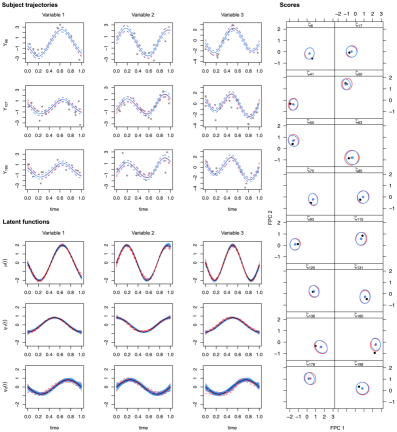
Figure 2: MCMC and VMP estimates for a problem with $p=3$ variables observed at an average of $15$ time points for $n=200$ subjects. Top left: estimated trajectories for a random subset of $3$ subjects, with posterior means (solid lines) and $95\%$ pointwise credible bands (dashed). The lines corresponding to MCMC (red) and VMP (blue) inference overlap. Bottom left: mean and eigen- functions simulated (black) and estimated by MCMC inference (red) with $95\%$ credible bands (dashed) and by VMP inference (blue) for which estimates from $100$ replicates are overlaid. Right: scores simulated (black dots) and estimated by MCMC (posterior mean, red dots) and VMP (posterior mean, blue dots) inference, with $95\%$ credible contours, for a random subset of $16$ subjects.

We start by evaluating the accuracy of the VMP algorithm through direct comparisons with MCMC and vanilla mean-field variational Bayes (MFVB) algorithms for the same model. While variational procedures use a prescribed tolerance, MCMC sampling requires evaluating the chain’s ability to explore the model space, which can be difficult for large problems. Since the two types of algorithms have different stopping rules and convergence diagnostics, comparing their accuracy and runtime can be challenging. To alleviate the risk of unfair comparisons, we conducted MCMC inference with the popular probabilistic programming language Stan (Carpenter et al., 2017), using the default no-U-turn sampler with $2\,000$ iterations of which $1\,000$ were discarded as burn-in.

Figure 2 shows the reconstructed trajectories and scores for randomly selected subjects, as well as the estimated latent functions, for a problem with $p=3$ variables, $n=200$ subjects and a number of observations drawn uniformly from the interval $[10,20]$ for each subject and each variable. It shows a very good agreement between the VMP and MCMC estimates. The same holds for comparisons between MFVB and MCMC estimates (Figure D.8 of Appendix D). Variational inference is known to be prone to posterior variance underestimation, especially when poor mean-field factorisations are employed (see, e.g., Blei et al., 2017); here however, the excellent agreement of the MCMC and variational credible bands for the estimated trajectories and scores provides empirical evidence that is issue is not encountered under the factorisation we employ. As expected the runtime is largely in favour of the variational procedure, with $20$ seconds for the VMP algorithm and $18$ minutes $28$ seconds for the MCMC algorithm on an Intel Xeon CPU, 2.60 GHz machine. The computational advantages of VMP inference over MCMC inference are discussed further in Section 5.6.

A comprehensive comparison of the errors on the estimated scores and latent functions for a grid of problems with $n\in\{50,100,200,300,400,500\}$ further shows strong agreement between the VMP, MFVB and MCMC, as well as a greater accuracy as $n$ increases (Figures D.9 & D.10 of Appendix D).

5.3 Comparison with frequentist multivariate FPCA

We next compare our Bayesian approach with the covariance-based frequentist multivariate approach proposed by Happ and Greven (2018). Here, we consider problems with $n=100$ subjects, for whom $p=3$ variables are measured longitudinally, with an average number of observations per subject and variable ranging from $20$ to $260$. Table 1 reports the ISE on the latent functions and the RMSE on the scores, based on $200$ replicates for each setting. Estimation accuracy is higher with our approach for the two eigenfunctions and comparable for the mean function, with a tendency for Happ and Greven (2018)’s method to improve as the average number of observations increases. A similar observation holds for the estimation of the two sets of scores. This aligns with the fact that our model-based Bayesian approach better handles sparse observation settings, as it eliminates the need for estimating and smoothing covariances, unlike conventional decomposition frequentist procedures, such as used in Happ and Greven (2018)’s approach. Moreover, while statistical performance becomes comparable for the two methods as the number of observations increases, the covariance-estimation requirement induces computational intractability for large covariance matrices, which prevents applications of Happ and Greven (2018)’s method on problems where the average number of observations per variable and subject exceeds $80$. We will provide a more comprehensive discussion of this computational limitation in Section 5.6.

For the setting where Happ and Greven (2018)’s method has the highest accuracy – namely, with $80$ observations per subject and variable, on average – the estimates obtained by the two approaches are visually very close (Figures D.11 & D.12 of Appendix D). An advantage of our approach is that posterior credible bands are readily obtained from the inferred variational posterior distributions. Such uncertainty estimates are unavailable using Happ and Greven (2018)’s method. Pointwise bootstrap confidence bands for the eigenvalues and eigenfunctions can be obtained, but the computational cost associated with the resampling becomes prohibitive for our problem sizes.

Average	$\mu(t)$		$\Psi_{1}(t)$		$\Psi_{2}(t)$		$\zeta_{1}$		$\zeta_{2}$
$n_{i}^{(j)}$	mFPCA	Happ	mFPCA	Happ	mFPCA	Happ	mFPCA	Happ	mFPCA	Happ
20	0.72 (0.73)	0.96 (0.57)	0.42 (0.27)	0.81 (0.41)	1.46 (0.82)	4.17 (2.55)	0.25 (0.05)	0.29 (0.03)	0.23 (0.03)	0.26 (0.03)
40	0.66 (0.82)	0.60 (0.42)	0.26 (0.20)	0.44 (0.27)	0.81 (0.43)	1.75 (0.88)	0.20 (0.07)	0.19 (0.03)	0.17 (0.03)	0.19 (0.02)
60	0.66 (0.96)	0.46 (0.50)	0.21 (0.21)	0.30 (0.22)	0.57 (0.30)	1.04 (0.44)	0.19 (0.09)	0.16 (0.04)	0.14 (0.03)	0.16 (0.03)
80	0.78 (0.93)	0.43 (0.46)	0.19 (0.21)	0.26 (0.24)	0.45 (0.35)	0.82 (0.40)	0.19 (0.11)	0.14 (0.05)	0.13 (0.04)	0.14 (0.03)
100	0.72 (1.08)	-	0.16 (0.16)	-	0.38 (0.21)	-	0.19 (0.13)	-	0.12 (0.03)	-
120	0.70 (1.06)	-	0.15 (0.18)	-	0.38 (0.20)	-	0.18 (0.13)	-	0.12 (0.03)	-
140	0.84 (1.27)	-	0.13 (0.19)	-	0.31 (0.24)	-	0.19 (0.14)	-	0.12 (0.04)	-
160	0.75 (0.95)	-	0.14 (0.23)	-	0.30 (0.25)	-	0.17 (0.13)	-	0.11 (0.04)	-
180	0.66 (1.04)	-	0.13 (0.19)	-	0.27 (0.23)	-	0.16 (0.14)	-	0.11 (0.05)	-
200	0.66 (1.20)	-	0.11 (0.19)	-	0.24 (0.19)	-	0.16 (0.14)	-	0.11 (0.06)	-
220	0.72 (1.15)	-	0.15 (0.19)	-	0.25 (0.22)	-	0.15 (0.14)	-	0.11 (0.05)	-
240	0.83 (1.21)	-	0.12 (0.22)	-	0.23 (0.23)	-	0.17 (0.15)	-	0.12 (0.06)	-
260	0.82 (1.42)	-	0.11 (0.21)	-	0.20 (0.22)	-	0.17 (0.15)	-	0.12 (0.07)	-

Table 1: Errors for latent functions (ISE $\times 100$) and scores (RMSE) estimated using our approach and Happ’s approach for a problem with $p=3$ variables, $n=100$ subjects, and average number of observations per variable and subject ranging from $20$ to $260$ (rows). The median and interquartile range (IQR, parentheses) obtained from $200$ data replicates are shown, and the smallest median error of each row is highlighted in bold. For $\mu(t)$, $\Psi_{1}(t)$ and $\Psi_{2}(t)$, and for each of the data replicates, the per-variable ISE are computed and averaged across the $p$ variables. A “-” indicates scenarios where simulations for Happ’s method fail to complete within $36$ hours (Intel Xeon CPU, 2.60 GHz).

5.4 Borrowing strength in sparse settings

We next examine the benefits of our hierarchical framework for handling estimation in complicated sparse-data settings, where borrowing information across variables and subjects is essential. Specifically, we simulate a problem with $n=200$ subjects and $p=6$ variables, of which the first is very scarcely observed (number of observations uniformly drawn in the interval $[5,10]$), while the remaining five variables are sampled more frequently (number of observations uniformly drawn in the interval $[50,75]$). We then apply our mFPCA approach jointly on the six variables, and compare the posterior estimates of the scores with those of separate univariate FPCA runs. Specifically, we conduct a series of six VMP runs, with $p=1$ in (7), and rescale their posterior mean and standard deviation by a factor $\sqrt{p}$ to make them orthonormal in the multivariate Hilbert space $\Hsc\equiv L^{2}([0,1])^{p}$.

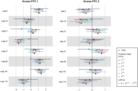
Figure 3: Posterior means with $95\%$ credible intervals for the scores obtained from univariate and multivariate Bayesian FPCA for a problem with $n=200$ subjects and $p=6$ variables, of which the first, $x^{(1)}$, is infrequently observed. Estimates are shown for random subset of $8$ subjects. The mFPCA estimates are in light red, the true simulated values are indicated by black triangles and the remaining colors correspond to estimates obtained from univariate FPCA runs.

In the previous section we have seen that the VMP algorithm advantageously provides uncertainty quantification for the estimated scores. Here we further examine the effect of pulling information with joint modelling on the credible bands and posterior means of the scores, placing special emphasis on the first variable which is infrequently observed. Figure 3 shows the estimated scores for the first and second principal components along with the $95\%$ credible intervals, for a random subset of $8$ subjects. All types of credible intervals tend to be larger for second principal component scores (FPC 2) compared to first principal component scores (FPC 1), reflecting the higher uncertainty associated with the former as they capture a smaller proportion of variance in the data. As expected, the small number of observations collected for the first variable leads to very wide the credible intervals for its corresponding scores (FPC 1 & 2) estimated with univariate FPCA. These intervals cover zero and some fail to include the true simulated scores (for subject 21 FPC 1 and subject 57 FPC 2). This suggests that this curve ($j=1$) is too infrequently observed in order for univariate FPCA to provide any meaningful and useful results. The remaining five curves ($j=2,\ldots,6$) are more frequently observed, and therefore the credible intervals of their corresponding univariate scores are narrower, yet in a few instances the true score is not covered (for $j=3$, subject 16 FPC 1 and subject 63 FPC 2).

Inspecting the credible intervals produced by the mFPCA approach suggests that borrowing strength effectively improves inference: (i) these intervals are generally substantially narrower than their univariate counterparts, and (ii) they all contain the true simulated score. This example shows how pulling information across variables and subjects observed at irregular temporal grids is particularly beneficial in settings where some variables entail very few measurements (here $j=1$). Another notable advantage of mFPCA is that it produces a single set of posterior estimates, under the form of scalar scores, for all variables (rather than six separate sets of scores here), thereby offering a very parsimonious summary of the temporal covariation in the multivariate data.

5.5 Performance under model misspecification

Borrowing information using joint approaches is sensible when the modelled variables are expected to covary over time. However assessing this can be difficult in practice. It is therefore important to evaluate the potential consequences on inference when this assumption is violated. In this section, we examine the robustness of our approach when the joint model is misspecified. Specifically, we generate $p$ variables from distinct univariate models, whose scores are simulated independently ($\rho=0$), or with varying degrees of correlation ($\rho=\{0.2,0.4,0.6,0.8\}$) up to complete correlation ($\rho=1$). This last case corresponds to no misspecification, since the data share the same set of scores and therefore can be thought as generated from the joint model (7). For each scenario, we compare the accuracy of our joint approach with its univariate counterpart, applied independently to each variable as in the previous section. We consider $100$ data replicates of a problem with $p=6$ variables, $n=50$ subjects, and with sparse observations drawn uniformly from the interval $[5,10]$ for each curve.

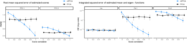
Figure 4: Comparison of the errors obtained using univariate and multivariate Bayesian FPCA for a problem with $p=6$ variables, $n=50$ subjects and numbers of observations drawn uniformly from the interval $[5,10]$ for each variable and each subject. The data were simulated from univariate FPCA models with varying degrees of score correlation $\rho\in\{0,0.2,0.4,0.6,0.8,1\}$ ($x$-axis). The median (dots) and first and third quartiles (grey) of the errors from $100$ data replicates are shown. Left: RMSE for the scores. For each data replicate, the univariate FPCA per-variable RMSE are computed and the average across all $p$ variables is shown. Right: ISE for the mean and eigen-functions. For each data replicate, and both univariate and multivariate FPCA, per-variable ISE are computed and the average across all $p$ variables is shown.

As anticipated, Figure 4 indicates a deterioration on the error of the scores using mFPCA as the correlation of the scores (FPC 1 & 2) weakens, to the point where the univariate model outperforms the joint model, for unrelated or weakly related variables where $\rho\in\{0,0.2,0.4\}$. However, the estimation of the latent functions is more robust to the misspecification, because, unlike the scores, the mean function and eigenfunctions are variable specific, which confers great flexibility, even under different latent dynamics for the $p$ variables. The fact that the ISE for the first eigenfunction is smaller under the joint model than under the univariate model when the correlation is weak ($\rho\leavevmode\nobreak\ \in\leavevmode\nobreak\ \{0.2,0.4\}$) can be attributed to the “virtually larger sample sizes” obtained by accounting jointly for the observations on all $p$ variables.

When the scores are more strongly correlated ($\rho\in\{0.6,0.8,1\}$), there is a substantial reduction in the RMSE of the scores, which is particularly striking for the first component. This again demonstrates the benefits of borrowing strength across related variables.

Altogether, these results suggest that the multivariate model is reasonably robust to misspecifications caused by a lack of common latent dynamics across the variables. Moreover, as shown in Section 5.4, when similar dynamics exist, joint modelling also tends to produce narrower credible intervals for the scores, which contain the true value.

5.6 Computational performance

As mentioned in the above numerical studies, our VMP algorithm has important computational advantages compared to other multivariate FPCA approaches. These advantages concern both runtime and memory (RAM) usages, and can be attributed to the combination of two features: (i) a direct, simultaneous inference of the Karhunen–Loève expansion, treating all parameters as unknown and estimating them jointly – this bypasses the need to model the covariance function, unlike with frequentist approaches which typically use a sequence of time- and memory-greedy smoothing and eigendecomposition steps to estimate large covariance functions; (ii) a fast, deterministic inference approach, which scales to large numbers of subjects and time points, unlike more conventional Bayesian inference approaches based on MCMC inference.

Figure 5 shows the runtime profiles corresponding to the simulations presented in Sections 5.2 and 5.3, on the logarithmic scale. It indicates that the VMP algorithm is $1$ to $2$ orders of magnitude faster than MCMC inference on the same model. The computational advantage of our algorithm compared the frequentist multivariate approach of Happ and Greven (2018) is as large, or perhaps even greater since the latter approach could not complete within $36$ hours for problems with an average number of observations per variable and subject exceeding $80$. For Happ and Greven (2018)’s approach, memory is also an important limiting factor, as the runs with $\leq 80$ observations required compute nodes with tens of GBs of RAM in order to store all matrix objects pertaining to the estimation of the covariance function.

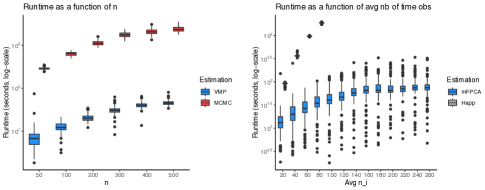
Figure 5: Runtime profiling (on the logarithmic scale) obtained on an Intel Xeon CPU, 2.60 GHz machine. Left: comparison of the MCMC (red) and VMP (blue) algorithms on the problems of Section 5.2 ($100$ replicates). Right: comparison of Happ’s (grey) and our (blue) approaches on the problems of Section 5.3 ($200$ replicates). The results for Happ’s method correspond to the four highest boxplots in black in bins $20$ to $80$; the method does not complete within $36$ hours for problems with more than $80$ observations per variable and subject, hence no boxplots are displayed.

6 The latent underpinnings of the immune response to SARS-CoV-2 infection

We return to the SARS-CoV-2 study presented in Section 2. As motivated there, since COVID-19 is a multi-system, heterogeneous disease, we will undertake to disentangle the patient variability of short- and long-term disease trajectories by applying mFPCA on molecular markers across several biological systems. Such an analysis will hopefully help us interpret the shared latent dynamics driving disease severity and incomplete organismal recovery.

Patient were categorised according to five clinical severity classes, based on their hospitalisation status and oxygen needs, namely, A, asymptomatic ($n=18$); B, mild symptomatic ($n=40$); C, hospitalised without supplemental oxygen ($n=50$); D, hospitalised with supplemental oxygen ($n=38$), and E, hospitalised with assisted ventilation ($n=69$). Time was measured from the first positive swab for patients of class A, and from symptom onset for patients of the remaining classes; to prevent biased inferences due to temporal shifts resulting from these different definitions, we focus our analysis on symptomatic patients, i.e., patients from classes B to E. We analyse data collected during the first $7$-weeks from symptom onset (acute and post-acute phase), focusing on five important molecular markers, namely, C-reactive protein (CRP) levels, interleukin 10 (IL-10) cytokine levels, glycoprotein B (glyc-B) levels and levels of two metabolites from the kynurenine pathway, quinolinic acid and tryptophan. We also further exclude patients that had fewer than two measurements collected within the $7$-week time window for any given marker, leaving a total of $n=82$ patients for analysis. Importantly, we are in presence of a complex sampling design, with sparse observations recorded at different time points across subjects and variables, which underlines the need for flexible hierarchical modelling with effective pooling of information. Finally, we use one-time measurements from $45$ SARS-CoV-2 negative healthy controls (HC), and use the IQR of the HC measurements for the five parameters as a reference for normal parameter levels.

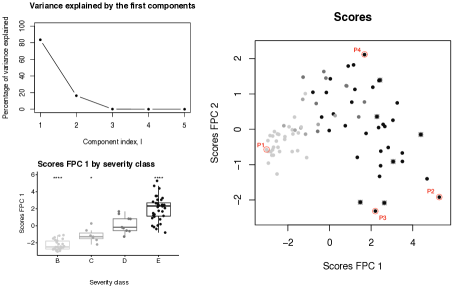
Figure 6: mFPCA analysis of the COVID-19 data. Top right: percentage of variance explained by the first $5$ components. The first two components capture $83.6\%$ and $16.3\%$ of the variance, respectively. Bottom right: FPC 1 scores (“severity scores”) as a function of the clinical severity classes B to E. Stars: one vs. all two-sided $t$-tests (${}^{****}:p<0.0001$, ${}^{***}:p<0.001$, ${}^{**}:p<0.01$ and ${}^{*}:p<0.05$). Right: estimates of the FPC 1 scores ($x$-axis, “severity scores”) and FPC 2 scores ($y$-axis, “recovery scores”). The red labels P1, P2, P3 and P4 indicate the patients with the most extreme severity or recovery scores, and the grey levels indicate the clinical severity classes B (light grey), C (grey), D (dark grey) or E (black) to which each patient belongs; the gradient of grey points along the $x$-axis again reflects the association of the FPC 1 scores with the severity classes. The six points with a black cross indicate patients who died from COVID-19.

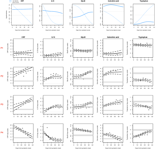
Figure 7: mFPCA analysis of the COVID-19 data: eigenfunctions and patient trajectories. Top row: first (blue) and second (light blue) eigenfunctions estimated for each marker (column) and displayed over the first $7$ weeks post symptom onset. Bottom rows: estimated trajectories (posterior mean with $95\%$ credible bands) for the four patients P1, P2, P3, P4 with most extreme scores as shown in Figure 6. The horizontal grey band corresponds to the healthy control (HC) IQR, reflecting normal levels of the corresponding markers.

We first set to determine the number of eigenfunctions needed to explain the temporal variation in the data. Analysing the data with $L=5$ components indicates a sharp decrease in variance explained after $l=2$ (Figure 6), with the first two components capturing together $>99\%$ of the variance; we therefore conduct the analysis with $L=2$ components. Convergence is obtained in $8$ seconds after $24$ iterations (Intel Xeon CPU, 2.60 GHz). Figure 7 shows that the two eigenfunctions estimated for the five markers have clear interpretations. Specifically, the first eigenfunction is above zero for CRP, IL-10, glyc-B and quinolinic acid, while it is below zero for tryptophan, over the entire $7$-week disease course. This means that patients with a positive score for the first eigenfunction tend to have positive deviations from the mean for the first four markers, and a negative deviation for tryptophan. This allows us to conclude that the scores corresponding to the first eigenfunction can serve as proxies for disease severity since it has been established that patients with severe COVID-19 infection tend to have increased levels of CRP, IL-10, glyc-B and quinolinic acid, and depleted tryptophan levels; in fact, these five markers have well-established roles in inflammation and immune regulation (Bergamaschi et al., 2021; Masuda et al., 2021). The second eigenfunction reflects parameter recovery over time, since it decreases for the first four markers and increases for tryptophan, meaning that patients with a positive score for the second eigenfunction tended to see their parameter disruption resolve over time, i.e., a decrease for the levels of the first four markers and an increase for tryptophan, toward normal levels.

Figure 6 displays the estimated patient scores corresponding to the two eigenfunctions. It suggests that the first set of scores reflects the clinical severity classes B to E, which corroborates their interpretation as proxies for disease severity, and this association is significant (anova $p<0.001$). Moreover, the group of six patients that did not survive had significantly higher scores for the first eigenfunction on average, compared to random patient groups of same size ($p<0.001$), and four of these six patients had negative scores for the second eigenfunction (poor recovery). We thus hereafter refer to the scores corresponding to the first and second eigenfunctions as “severity” and “recovery” scores, respectively.

Figure 7 shows the reconstructed parameter trajectories for four patients with extreme scores (referred to as “P1”, “P2”, “P3” and “P4” in Figure 6). They also corroborate the interpretation on the scores, since the trajectories of patient P1, with the most favourable severity and recovery scores, largely overlap the normal HC range over the entire disease course. The trajectories of patient P2, with a high severity score, tend to stay well above (or below, for tryptophan) the normal range. Finally, the trajectories of patient P3 (P4), with unfavourable (favourable) recovery scores, tend to deteriorate (resolve) over time, as expected.

mFPCA	Severity scores		Recovery scores
Dyspnoea	0.34	*	0.28	.
Cough	0.3	*	0.21
Chest Pain on exertion, palpitations or swollen ankles	0.1		0.08
New leg swelling in one leg or shortness of breath with chest pain	0.12		0.05
New skin rashes or sores	0.23		0.26	.
Voice alteration	0.21		0.24
Difficulties eating, drinking or swallowing	0.18		-0.02
Constant noisy breathing or throat whistling	0.02		0.08
Anosmia or dysgeusia	0.08		0.1
Difficulty to gain or maintain weight, loss of appetite	0.03		0
New neurology in one or more limbs	0.33	*	0.18
New pain in one or more parts of the body	0.49	***	0.39	*
General muscle weakness, balance or range of movement of joints	0.43	**	0.26	.
Fatigue	0.36	**	0.33	*
Cognition: memory, concentration and thinking skills	0.09		0.23
Overall physical & mental recovery:
mFPCA (n = 40)	0.39	**	0.32	**
FPCA CRP (n = 51)	0.28	**	0.14
FPCA IL-10 (n = 40)	0.29	*	0.16
FPCA GlycB (n = 57)	0.22	*	0.02
FPCA Quinolinic acid (n = 57)	0.27	**	0.04
FPCA Tryptophan (n = 57)	0.15		0.12

Table 2: Association of the scores with long-COVID symptoms. Kendall’s rank correlation and significance after Benjamini–Hochberg multiplicity adjustment (^∗∗∗: FDR$<0.001$, ^∗∗: FDR$<0.01$ and ${}^{*}:$ FDR$<0.05$, ${}^{.}:$ FDR$<0.1$) for the association of the severity and recovery mFPCA scores with long-COVID symptoms ranked from $0$ (no symptom) to $5$ (extreme manifestation of the symptom). Kendall’s rank correlation and significance with overall physical and mental recovery is also assessed for scores estimated by separate univariate FPCA analysis; the sample size for the tests are indicated and correspond to the intersection of the number of patients used in each FPCA/mFPCA analysis and the number patients for which long-COVID questionnaires were collected.

We next use survival data and questionnaires collected up to one year after infection to ask whether the latent dynamics underlying the disease courses over the first $7$ weeks post symptom onset are associated with fatalities and specific long-COVID symptoms. The six patients who did not survive were all under assisted ventilation (class E) and died at $19$, $20$, $44$, $109$, $153$ and $158$ days post symptom onset, respectively. Using a Cox proportional hazards model, we find that severity scores are significantly associated with survival ($p=0.005$), but not the recovery scores ($p=0.15$), which suggests that peak severity during the acute and post-acute phases has greater prognostic value than the actual disease dynamics. Table 2 next shows associations of the severity and recovery scores with specific long-COVID symptoms that were evaluated for a subset of $67$ patients on a scale from $0$ (no symptom) to $5$ (extreme manifestation of the symptom). Using Kendall’s rank correlation tests and a Benjamini–Hochberg multiplicity correction of $5\%$, severity scores are associated with six long-term symptoms, namely, dyspnoea, cough and four neurological symptoms, while recovery scores are associated with fatigue and pain. Moreover, both sets of severity and recovery scores are associated with an “Overall physical and mental recovery” category recorded in all patient questionnaires ($p=0.001$ and $p=0.007$, respectively; Table 2).

Finally, we explore the extent to which the analysis benefits from borrowing information across the five markers using our mFPCA approach, by inspecting whether added biological insights are obtained compared to separate univariate FPCA analyses. To this end, we perform independent runs of the univariate version of our Bayesian approach ($p=1$) for each of the five markers. Except for the IL-10 analysis, the number of patients analysed is larger than for the multivariate analysis as it is not limited by the threshold $\geq 2$ on the number of observations across all five markers (i.e., we have CRP: $n=96$, IL-10: $n=82$, glyc-B: $n=106$, quinolinic acid: $n=106$ and tryptophan: $n=106$). Interestingly, in each univariate analysis, the scores corresponding to the first two eigenfunctions have the same interpretation as in the multivariate analysis, that is, they are proxies of severity and recovery, respectively. However, as shown in Table 2, inspecting their association with long-term recovery indicates that, while nearly all sets of univariate severity scores (except for tryptophan) are significantly associated with the “Overall physical and mental recovery” category, none of the univariate recovery scores are associated with it. This suggests that the joint analysis better captures the underlying latent dynamics reflecting recovery patterns, since associations with the mFPCA severity and recovery scores are both highly significant, as discussed above. Finally, as already emphasised in the different simulation studies, the fact that mFPCA provides single set of scalar scores, FPC 1 and FPC 2, common to all five markers, allows effectively summarising their temporal covariation, unlike with univariate FPCA which yields separate sets of scores for the different markers, hindering the ability to grasp a synthetic picture.

7 Discussion

We have presented a hierarchical modelling framework for multivariate functional principal component analysis (mFPCA) using variational message passing (VMP) inference, which addresses important challenges posed in complex real-world sampling designs, by flexibly pooling information from limited data and infrequently observed curves. This is, to the best of our knowledge, the first Bayesian approach to mFPCA.

We model the temporal covariation of multivariate curves via the model hierarchy, namely, via shared scores which allow borrowing strength across related longitudinal measurements. In addition to enhancing statistical power, this model-based approach circumvents the estimation of large covariance and cross-covariance matrices, and thus enables mFPCA in (i) sparse and irregular sampling settings and (ii) sizable real-data settings which are typically beyond the scope of existing frequentist mFPCA approaches. Variational inference using message passing permits an elegant modularisation of the algorithm algebra under the form of fragments. Thanks to this principle, we could seamlessly repurpose fragments obtained in our previous work (Nolan et al., 2023) and combine them with a newly-derived multivariate functional principal component Gaussian likelihood fragment. This new fragment, on its own, constitutes a novel contribution, with utility extending beyond the present work context: its algebraic derivation and computer code are now readily available to statisticians willing to employ VMP inference for any models involving multivariate Gaussian likelihood components.

Our detailed simulation studies indicate that the VMP algorithm is both accurate and computationally efficient: it produces comparable or lower estimation errors on the scores and latent functions compared to MCMC inference on the same model and to the frequentist approach of Happ and Greven (2018), while being orders of magnitude faster. Crucially, we have seen how our hierarchical model allowed estimation from data with very sparsely observed curves ($5$-$10$ observations), exploiting information about other related curves with sampling grids that differ across variables and subjects.

In addition to its accuracy, flexibility and computational convenience, our Bayesian mFPCA framework possesses important advantages in terms of interpretability and uncertainty quantification. The “shared score” parametrisation offers a parsimonious representation of the major modes of joint variation of the curves, and our VMP procedure approximates the full posterior distribution of the scores, making it straightforward to construct credible boundaries. These scores therefore constitute a principled, subject-level scalar summary of the multivariate curves that can be used for further analysis tasks, such as regression or clustering. We have illustrated such a use case in the COVID-19 study where we inspected the association of patient-specific “severity” (FPC 1) and “recovery” (FPC 2) scores estimated from related molecular markers, with survival outcomes and long-term symptoms. Specifically, our mFPCA framework highlighted complex coordinated dynamics across the inflammatory, immune and metabolic systems, and suggested that the patients’ molecular status during the acute and post-acute phase is interlinked with incomplete clinical recovery up to one year post disease onset. This should prompt further research on organismal recovery from COVID-19, to pinpoint the specific inflammatory and immune mechanisms mobilised early in the disease course, understand their possible long-term consequences, and help formulate therapeutic recommendations applicable soon after infection to prevent adverse outcomes.

Thanks to its versatility and scalability, our framework is readily applicable to any study that involves multiple parameters measured longitudinally, possibly with scarce and irregular observations across subjects and functional curves. We anticipate that frameworks like ours will gain relevance in the near future for acquiring early personalised insights into disease risk, development and monitoring, especially when applied to routinely collected blood test data (complete blood count or CBC) available from electronic health records.

There are several avenues for methodological development. One of them concerns extensions to high-dimensional curves, a setting which is expected to gain prominence; for instance, in genomics, there is growing interest in collecting longitudinal observations on a large number of genes (up to $20\,000$ within the human genome) to understand how dynamic gene expression programs drive disease formation.

Software

The R package bayesFPCA is available at https://github.com/hruffieux/bayesFPCA.

Data

The data and metadata for the SARS-CoV-2 study are available at NIHR CITIID COVID-19 Cohort (https://www.covid19cellatlas.org/patient/citiid/).

Funding

This research was supported by the the Wellcome Collaborative Award 219506/Z/19/Z (T.N.), the UK Medical Research Council programme MRC MC UU 00002/10 (S.R.), the Alan Turing Institute, London, UK (S.R.) and the Lopez–Loreta Foundation (H.R.).

Appendix

Matrix algebraic background

We define the $\vect$ and $\vech$ operators, which are well-established (Gentle, 2007, e.g.). For a $d_{1}\times d_{2}$ matrix, the $\vect$ operator concatenates the columns of the matrix from left to right. For a $d_{1}\times d_{1}$ matrix, the $\vech$ operator concatenates the columns of the matrix after removing the above diagonal elements. For example, suppose that $\bA=[\begin{array}[]{c c}\T{(2,-3)}&\T{(-1,1)}\end{array}]$. Then $\vect(\bA)=\T{(2,-3,-1,1)}$ and $\vech(\bA)=\T{(2,-3,1)}$. For a $d^{2}\times 1$ vector $\ba$, $\vect^{-1}(\ba)$ is the $d\times d$ matrix such that $\vect\{\vect^{-1}(\ba)\}=\ba$. Additionally, the matrix $\bD_{d}$ is the duplication matrix of order $d$, and it is such that $\bD_{d}\vech(\bA)=\vect(\bA)$ for a $d\times d$ symmetric matrix $\bA$. Furthermore, $\bD_{d}^{+}\equiv(\T{\bD_{d}}\bD_{d})^{-1}\T{\bD_{d}}$ is the Moore-Penrose inverse of $\bD_{d}$, where $\bD_{d}^{+}\vect(\bA)=\vech(\bA)$.

For a set of $d$ matrices $\{\bM_{i}\}_{i=1,\dots,d}$, we define:

$$\stack_{i=1,\dots,d}(\bM_{i})\equiv\begin{bmatrix}\bM_{1}\\ \vdots\\ \bM_{d}\end{bmatrix}\quad\text{and}\quad\blockdiag_{i=1,\dots,d}(\bM_{i})\equiv\begin{bmatrix}\bM_{1}&\bO&\cdots&\bO\\ \bO&\bM_{2}&\cdots&\bO\\ \vdots&\vdots&\ddots&\vdots\\ \bO&\bO&\cdots&\bM_{d}\end{bmatrix},$$

with the first of these definitions requiring that each $\bM_{i}$ has the same number of columns.

Appendix A Proof of Proposition 4.1

First, set $\btheta\equiv\{\bnu,\bzeta_{1},\dots,\bzeta_{n},\bsigma_{\epsilon}^{2},\ba_{\epsilon},\bsigma_{\mu}^{2},\ba_{\mu},\bsigma_{\psi_{1}}^{2},\dots,\bsigma_{\psi_{L}}^{2},\ba_{\psi_{1}},\dots,\ba_{\psi_{L}}\}$, the entire parameter set. Then, the optimal posterior density function for $\bnu$ in (8) that minimises the Kullback–Leibler divergence of its left-hand side from its right-hand side is computed according to

$$q(\bnu)=C_{1}\exp\left\{\E_{q(\btheta\setminus\bnu)}\log p(\bx,\btheta)\right\},$$ (15)

where $C_{1}$ is a constant of proportionality. Next, note that

$$\log p(\bx,\btheta)=\sum_{j=1}^{p}\left\{\sum_{i=1}^{n}\log p(\bx_{i}^{(j)}\mid\bnu^{(j)},\bzeta_{i},\sigma^{(j)2}_{\epsilon})+\log p(\bnu^{(j)}\mid\sigma^{((j))2}_{\epsilon})\right\}+f(\btheta\setminus\bnu),$$ (16)

where $\bx^{(j)}\equiv\T{(\bx_{1}^{(j)\intercal},\dots,\bx_{n}^{(j)\intercal})}$, for $j=1,\dots,p$, and $f(\btheta\setminus\bnu)$ represents an arbitrary function that does not depend on $\bnu$. Substituting (16) into (15), we have

$$q(\bnu)=C_{2}\prod_{j=1}^{p}\exp\left[\E_{q(\btheta\setminus\bnu^{(j)})}\left\{\sum_{i=1}^{n}\log p(\bx_{i}^{(j)}\mid\bnu^{(j)},\bzeta_{i},\sigma^{(j)2}_{\epsilon})+\log p(\bnu^{(j)}\mid\sigma^{((j))2}_{\epsilon})\right\}\right]=\prod_{j=1}^{p}q(\bnu^{(j)}),$$

where $C_{2}$ is an arbitrary constant of proportionality.

Appendix B Exponential family form

We first describe the exponential family form for the normal distribution. For a $d\times 1$ multivariate normal random vector $\bx\sim\normal(\bmu,\bSigma)$, the probability density function of $\bx$ can be shown to satisfy

$$p(\bx)=\exp\left\{\T{\bT_{\vect}(\bx)}\bdeta_{\vect}-A_{\vect}(\bdeta_{\vect})-\frac{d}{2}\log(2\pi)\right\},$$ (17)

where $\bT_{\vect}(\bx)\equiv\T{\{\T{\bx},\T{\vect(\bx\T{\bx})}\}}$ is the vector of sufficient statistics and $\bdeta_{\vect}\equiv\T{(\T{\bdeta_{\vect,1}},\T{\bdeta_{\vect,2}})}\equiv\T{[\T{(\bSigma^{-1}\bmu)},-\frac{1}{2}\T{\{\vect(\bSigma^{-1})\}}]}$ is the natural parameter vector. The function $A_{\vect}(\bdeta_{\vect})=-\frac{1}{4}\T{\bdeta}_{\vect,1}\{\vect^{-1}(\bdeta_{\vect,2})\}^{-1}\bdeta_{\vect,1}-\frac{1}{2}\log|-2\vect^{-1}(\bdeta_{\vect,2})|$ is the log-partition function. The inverse mapping of the natural parameter vector is (Wand, 2017, equation S.4)

$$\bmu=-\frac{1}{2}\left\{\vect^{-1}(\bdeta_{\vect,2})\right\}^{-1}\bdeta_{\vect,1}\quad\text{and}\quad\bSigma=-\frac{1}{2}\left\{\vect^{-1}(\bdeta_{\vect,2})\right\}^{-1}.$$ (18)

We will refer to the representation of the multivariate normal probability density function in (17) as the vec-based representation.

Alternatively, a more storage-economical representation of the multivariate normal probability density function is the vech-based representation:

$$p(\bx)=\exp\left\{\T{\bT_{\vech}(\bx)}\bdeta_{\vech}-A_{\vech}(\bdeta_{\vech})-\frac{d}{2}\log(2\pi)\right\},$$

where the vector of sufficient statistics, the natural parameter vector and the log-partition function are, $\bT_{\vech}(\bx)\equiv\T{\{\T{\bx},\T{\vect(\bx\T{\bx})}\}}$, $\bdeta_{\vech}\equiv\T{(\T{\bdeta_{\vech,1}},\T{\bdeta_{\vech,2}})}\equiv\T{[\T{(\bSigma^{-1}\bmu)},\allowbreak-\frac{1}{2}\T{\T{\bD_{d}}\{\vect(\bSigma^{-1})\}}]}$ and $A_{\vech}(\bdeta_{\vech})=-\frac{1}{4}\T{\bdeta}_{\vech,1}\{\vect^{-1}(\bD_{d}^{+\intercal}\bdeta_{\vech,2})\}^{-1}\bdeta_{\vech,1}-\frac{1}{2}\log|-2\vect^{-1}(\bD_{d}^{+\intercal}\bdeta_{\vech,2})|$, respectively. The inverse mapping of the natural parameter vector under the vech-based representation is

$$\bmu=-\frac{1}{2}\left\{\vect^{-1}(\bD_{d}^{+\intercal}\bdeta_{\vech,2})\right\}^{-1}\bdeta_{\vech,1}\quad\text{and}\quad\bSigma=-\frac{1}{2}\left\{\vect^{-1}(\bD_{d}^{+\intercal}\bdeta_{\vech,2})\right\}^{-1}.$$ (19)

The other major distribution within the exponential family that is pivotal for this article is the inverse-$\chi^{2}$ distribution. A random variable $x$ has an inverse-$\chi^{2}$ distribution with shape parameter $\xi>0$ and scale parameter $\lambda>0$ if the probability density function of $x$ is

$$p(x)=\frac{(\lambda/2)^{\xi/2}}{\Gamma(\xi/2)}x^{-(\xi+2)/2}\exp\left(-\frac{\lambda}{2x}\right)\ind(x>0),$$

where the vector of sufficient statistics, the natural parameter vector and the log-partition function are $\bT(x)\equiv\T{(\log(x),1/x)}$, $\bdeta=\T{(\eta_{1},\eta_{2})}=\T{\{-\frac{1}{2}(\xi+2),-\frac{\lambda}{2}\}}$ and $A(\bdeta)\equiv\log\{\Gamma(\xi/2)\}-\frac{\xi}{2}\log(\lambda/2)$, respectively. Note that $\Gamma(z)\equiv\int_{0}^{\infty}u^{z-1}e^{u}du$ is the gamma function, $\ind(\cdot)$ is the indicator function, $\zeta>0$ is the scale parameter and $\lambda>0$ is the shape parameter. The inverse mapping of the natural parameter vector is $\xi=-2\eta_{1}-2$ and $\lambda=-2\eta_{2}$.

Appendix C Derivation of the multivariate functional principal component Gaussian likelihood fragment

From (7), we have, for $i=1,\dots,n$ and $j=1,\dots,p$,

$$\log p(\bx_{i}^{(j)}|\bnu^{(j)},\bzeta_{i},\sigma^{(j)2}_{\epsilon})=-\frac{n_{i}^{(j)}}{2}\log(\sigma^{(j)2}_{\epsilon})-\frac{1}{2\sigma^{(j)2}_{\epsilon}}\left|\left|\bx_{i}^{(j)}-\bC_{i}^{(j)}\left(\bnu_{\mu}^{(j)}+\sum_{l=1}^{L}\zeta_{il}\bnu_{\psi_{l}}^{(j)}\right)\right|\right|^{2}+\text{const.}$$ (20)

First, we establish the natural parameter vector for each of the optimal posterior density functions. These natural parameter vectors are essential for determining expectations with respect to the optimal posterior distribution. From equation (10) of Wand (2017), we deduce that the natural parameter vector for $q(\bnu^{(j)})$, $j=1,\dots,p$ is

$$\npq{\bnu^{(j)}}=\np{p(\bx\mid\bnu,\bzeta_{1},\dots,\bzeta_{n},\sigma^{(1)2}_{\epsilon},\dots,\sigma^{(p)2}_{\epsilon})}{\bnu^{(j)}}+\np{\bnu^{(j)}}{p(\bx\mid\bnu,\bzeta_{1},\dots,\bzeta_{n},\sigma^{(1)2}_{\epsilon},\dots,\sigma^{(p)2}_{\epsilon})},$$

the natural parameter vector for $q(\bzeta_{i})$, $i=1,\dots,n$, is

$$\npq{\bzeta_{i}}=\np{p(\bx\mid\bnu,\bzeta_{1},\dots,\bzeta_{n},\sigma^{(1)2}_{\epsilon},\dots,\sigma^{(p)2}_{\epsilon})}{\bzeta_{i}}+\np{\bzeta_{i}}{p(\bx\mid\bnu,\bzeta_{1},\dots,\bzeta_{n},\sigma^{(1)2}_{\epsilon},\dots,\sigma^{(p)2}_{\epsilon})},$$

and the natural parameter vector for $q(\sigma^{(j)2}_{\epsilon})$, $j=1,\dots,p$ is

$$\npq{\sigma^{(j)2}_{\epsilon}}=\np{p(\bx\mid\bnu,\bzeta_{1},\dots,\bzeta_{n},\sigma^{(1)2}_{\epsilon},\dots,\sigma^{(p)2}_{\epsilon})}{\sigma^{(j)2}_{\epsilon}}+\np{\sigma^{(j)2}_{\epsilon}}{p(\bx\mid\bnu,\bzeta_{1},\dots,\bzeta_{n},\sigma^{(1)2}_{\epsilon},\dots,\sigma^{(p)2}_{\epsilon})}.$$

Next, we consider the updates for standard expectations that occur for each of the random variables and random vectors in (20). For each $\bnu^{(j)}$, we need to determine the mean vector $\E_{q}(\bnu^{(j)})$ and the covariance matrix $\Cov_{q}(\bnu^{(j)})$. The expectations are taken with respect to the normalisation of

$$\msg{p(\bx\mid\bnu,\bzeta_{1},\dots,\bzeta_{n},\sigma^{(1)2}_{\epsilon},\dots,\sigma^{(p)2}_{\epsilon})}{\bnu^{(j)}}(\bnu^{(j)})\ \msg{\bnu^{(j)}}{p(\bx\mid\bnu,\bzeta_{1},\dots,\bzeta_{n},\sigma^{(1)2}_{\epsilon},\dots,\sigma^{(p)2}_{\epsilon})}(\bnu^{(j)}),$$

which is a multivariate normal density function with natural parameter vector $\npq{\bnu^{(j)}}$. From (18), we have

$$\begin{split}\E_{q}(\bnu^{(j)})&\longleftarrow-\frac{1}{2}\left[\vect^{-1}\left\{\left(\npq{\bnu^{(j)}}\right)_{2}\right\}\right]^{-1}\left(\npq{\bnu^{(j)}}\right)_{1}\\ \text{and}\quad\Cov_{q}(\bnu^{(j)})&\longleftarrow-\frac{1}{2}\left[\vect^{-1}\left\{\left(\npq{\bnu^{(j)}}\right)_{2}\right\}\right]^{-1}.\end{split}$$ (21)

Furthermore, the mean vector has the form

$$\E_{q}(\bnu^{(j)})\equiv\T{\left\{\T{\E_{q}(\bnu_{\mu}^{(j)})},\T{\E_{q}(\bnu_{\psi_{1}}^{(j)})},\dots,\T{\E_{q}(\bnu_{\psi_{L}}^{(j)})}\right\}},$$ (22)

and the covariance matrix has the form

$$\Cov_{q}(\bnu)\equiv\begin{bmatrix}\Cov_{q}(\bnu_{\mu}^{(j)})&\Cov_{q}(\bnu_{\mu}^{(j)},\bnu_{\psi_{1}}^{(j)})&\dots&\Cov_{q}(\bnu_{\mu}^{(j)},\bnu_{\psi_{L}}^{(j)})\\ \Cov_{q}(\bnu_{\psi_{1}}^{(j)},\bnu_{\mu}^{(j)})&\Cov_{q}(\bnu_{\psi_{1}}^{(j)})&\dots&\Cov_{q}(\bnu_{\psi_{1}}^{(j)},\bnu_{\psi_{L}}^{(j)})\\ \vdots&\vdots&\ddots&\vdots\\ \Cov_{q}(\bnu_{\psi_{L}}^{(j)},\bnu_{\mu}^{(j)})&\Cov_{q}(\bnu_{\psi_{L}}^{(j)},\bnu_{\psi_{1}}^{(j)})&\dots&\Cov_{q}(\bnu_{\psi_{L}}^{(j)})\\ \end{bmatrix}.$$ (23)

Similarly, for each $i=1,\dots,n$, we need to determine the optimal mean vector and covariance matrix for $\bzeta_{i}$, which are $\E_{q}(\bzeta_{i})$ and $\Cov_{q}(\bzeta_{i})$, respectively. The expectations are taken with respect to the normalisation of

$$\msg{p(\bx\mid\bnu,\bzeta_{1},\dots,\bzeta_{n},\sigma^{(1)2}_{\epsilon},\dots,\sigma^{(p)2}_{\epsilon})}{\bzeta_{i}}(\bzeta_{i})\ \msg{\bzeta_{i}}{p(\bx\mid\bnu,\bzeta_{1},\dots,\bzeta_{n},\sigma^{(1)2}_{\epsilon},\dots,\sigma^{(p)2}_{\epsilon})}(\bzeta_{i}),$$

which is a multivariate normal density function with natural parameter vector $\npq{\bzeta_{i}}$. According to (19),

$$\begin{split}\E_{q}(\bzeta_{i})&\longleftarrow-\frac{1}{2}\left[\vect^{-1}\left\{\bD_{L}^{+\intercal}\left(\npq{\bzeta_{i}}\right)_{2}\right\}\right]^{-1}\left(\npq{\bzeta_{i}}\right)_{1}\\ \text{and}\quad\Cov_{q}(\bzeta_{i})&\longleftarrow-\frac{1}{2}\left[\vect^{-1}\left\{\bD_{L}^{+\intercal}\left(\npq{\bzeta_{i}}\right)_{2}\right\}\right]^{-1},\quad\text{for $i=1,\dots,n$.}\end{split}$$ (24)

Finally, for each $j=1,\dots,p$, we need to determine $\E_{q}(1/\sigma^{(j)2}_{\epsilon})$, with the expectation taken with respect to the normalisation of

$$\msg{p(\bx\mid\bnu,\bzeta_{1},\dots,\bzeta_{n},\sigma^{(1)2}_{\epsilon},\dots,\sigma^{(p)2}_{\epsilon})}{\sigma^{(j)2}_{\epsilon}}(\sigma^{(j)2}_{\epsilon})\ \msg{\sigma^{(j)2}_{\epsilon}}{p(\bx\mid\bnu,\bzeta_{1},\dots,\bzeta_{n},\sigma^{(1)2}_{\epsilon},\dots,\sigma^{(p)2}_{\epsilon})}(\sigma^{(j)2}_{\epsilon}).$$

This is an inverse-$\chi^{2}$ density function, with natural parameter vector $\npq{\sigma^{(j)2}_{\epsilon}}$. According to Result 6 of Maestrini and Wand (2020),

$$\E_{q}(1/\sigma^{(j)2}_{\epsilon})\longleftarrow\frac{\left(\npq{\sigma^{(j)2}_{\epsilon}}\right)_{1}+1}{\left(\npq{\sigma^{(j)2}_{\epsilon}}\right)_{2}}.$$

Now, we turn our attention to the derivation of the message passed from $p(\bx\mid\bnu,\bzeta_{1},\dots,\bzeta_{n},\sigma^{(1)2}_{\epsilon},\dots,\sigma^{(p)2}_{\epsilon})$ to $\bnu^{(j)}$, $j=1,\dots,p$. Notice that

$$\bC_{i}^{(j)}\left(\bnu_{\mu}^{(j)}-\sum_{l=1}^{L}\zeta_{il}\bnu_{\psi_{l}}^{(j)}\right)=(\T{\bzetatilde_{i}}\otimes\bC_{i}^{(j)})\bnu^{(j)}.$$ (25)

Therefore, as a function of $\bnu^{(j)}$, (20) can be re-written as

$$\log p(\bx_{i}^{(j)}\mid\bnu^{(j)},\bzeta_{i},\sigma^{(j)2}_{\epsilon}) =-\frac{1}{2\sigma^{(j)2}_{\epsilon}}\left|\left|\bx_{i}^{(j)}-(\T{\bzetatilde_{i}}\otimes\bC_{i}^{(j)})\bnu^{(j)}\right|\right|^{2}+\text{terms not involving $\bnu^{(j)}$}$$

$$=\T{\begin{bmatrix}\bnu^{(j)}\\ \vect(\bnu^{(j)}\bnu^{(j)\intercal})\end{bmatrix}}\begin{bmatrix}\frac{1}{\sigma^{(j)2}_{\epsilon}}\T{(\T{\bzetatilde_{i}}\otimes\bC_{i}^{(j)})}\bx_{i}^{(j)}\\ -\frac{1}{2\sigma^{(j)2}_{\epsilon}}\vect\left\{(\bzetatilde_{i}\T{\bzetatilde_{i}})\otimes(\bC_{i}^{(j)\intercal}\bC_{i}^{(j)})\right\}\end{bmatrix}$$

$$\qquad+\text{terms not involving $\bnu^{(j)}$}.$$

According to equation (8) of Wand (2017), the message from the factor $p(\bx\mid\bnu,\bzeta_{1},\dots,\bzeta_{n},\sigma^{(1)2}_{\epsilon},\dots,\sigma^{(p)2}_{\epsilon})$ to $\bnu^{(j)}$ is

$$\msg{p(\bx\mid\bnu,\bzeta_{1},\dots,\bzeta_{n},\sigma^{(1)2}_{\epsilon},\dots,\sigma^{(p)2}_{\epsilon})}{\bnu^{(j)}}(\bnu^{(j)})\propto\exp\left\{\T{\begin{bmatrix}\bnu^{(j)}\\ \vect(\bnu^{(j)}\bnu^{(j)\intercal})\end{bmatrix}}\np{p(\bx\mid\bnu,\bzeta_{1},\dots,\bzeta_{n},\sigma^{(1)2}_{\epsilon},\dots,\sigma^{(p)2}_{\epsilon})}{\bnu^{(j)}}\right\},$$

which is proportional to a multivariate normal density function. The update for the message’s natural parameter vector, in (11), is dependent upon the mean vector and covariance matrix of $\bzetatilde_{i}$, which are

$$\E_{q}(\zetatilde_{i})=\T{\{1,\T{\E_{q}(\bzeta_{i})}\}}\quad\text{and}\quad\Cov_{q}(\zetatilde_{i})=\blockdiag\left\{0,\Cov_{q}(\bzeta_{i})\right\},\quad\text{for $i=1,\dots,n$,}$$ (26)

where $\E_{q}(\bzeta_{i})$ and $\Cov_{q}(\bzeta_{i})$ are defined in (24). Note that a standard statistical result allows us to write

$$\E_{q}(\bzetatilde_{i}\T{\bzetatilde_{i}})=\Cov_{q}(\bzetatilde_{i})+\E_{q}(\bzetatilde_{i})\T{\E_{q}(\bzetatilde_{i})},\quad\text{for $i=1,\dots,n$.}$$ (27)

Next, notice that

$$\sum_{l=1}^{L}\zeta_{il}\bnu_{\psi_{l}}^{(j)}=\bV_{\psi}^{(j)}\bzeta_{i}$$ (28)

Then, for each $i=1,\dots,n$, the log-density function in (20) can be represented as a function of $\bzeta_{i}$ by

$$\log p(\bx_{i}^{(j)}\mid\bnu^{(j)},\bzeta_{i},\sigma^{(j)2}_{\epsilon}) =-\frac{1}{2\sigma^{(j)2}_{\epsilon}}\left|\left|\bx_{i}^{(j)}-\bC_{i}^{(j)}\bnu_{\mu}^{(j)}-\bC_{i}^{(j)}\bV_{\psi}^{(j)}\bzeta_{i}\right|\right|^{2}+\text{terms not involving $\bzeta_{i}$}$$

$$=\T{\begin{bmatrix}\bzeta_{i}\\ \vech(\bzeta_{i}\T{\bzeta_{i}})\end{bmatrix}}\begin{bmatrix}\frac{1}{\sigma^{(j)2}_{\epsilon}}(\bV_{\psi}^{(j)\intercal}\bC_{i}^{(j)\intercal}\bx_{i}^{(j)}-\bh_{\mu\psi,i}^{(j)})\\ -\frac{1}{2\sigma^{(j)2}_{\epsilon}}\T{\bD_{L}}\vect(\bH_{\psi,i}^{(j)})\end{bmatrix}$$

$$\qquad+\text{terms not involving $\bzeta_{i}$},$$

According to equation (8) of Wand (2017), the message from the factor $p(\bx\mid\bnu,\bzeta_{1},\dots,\bzeta_{n},\sigma^{(1)2}_{\epsilon},\dots,\sigma^{(p)2}_{\epsilon})$ to $\bzeta_{i}$ is

$$\msg{p(\bx\mid\bnu,\bzeta_{1},\dots,\bzeta_{n},\sigma^{(1)2}_{\epsilon},\dots,\sigma^{(p)2}_{\epsilon})}{\bzeta_{i}}(\bzeta_{i})\propto\exp\left\{\T{\begin{bmatrix}\bzeta_{i}\\ \vech(\bzeta_{i}\T{\bzeta_{i}})\end{bmatrix}}\np{p(\bx\mid\bnu,\bzeta_{1},\dots,\bzeta_{n},\sigma^{(1)2}_{\epsilon},\dots,\sigma^{(p)2}_{\epsilon})}{\bzeta_{i}}\right\},$$

which is proportional to a multivariate normal density function. The message’s natural parameter vector update, in (12), is dependant on the following expectations that are yet to be determined:

$$\E_{q}(\bV_{\psi}^{(j)}),\quad\E_{q}(\bH_{\psi,i}^{(j)}),\quad\text{and}\quad\E_{q}(\bh_{\mu\psi,i}^{(j)}),\quad i=1,\dots,n\quad\text{and}\quad j=1,\dots,p.$$

Now, we have,

$$\E_{q}(\bV_{\psi}^{(j)})=\begin{bmatrix}\E_{q}(\bnu_{\psi_{1}}^{(j)})&\dots&\E_{q}(\bnu_{\psi_{L}}^{(j)})\end{bmatrix},$$ (29)

where, for $l=1,\dots,L$, $\E_{q}(\bnu_{\psi_{l}}^{(j)})$ is defined by (21) and (22). Next, $\E_{q}(\bh_{\mu\psi,i}^{(j)})$ is an $L\times 1$ vector, with $l$th component being

$$\E_{q}(\bh_{\mu\psi,i}^{(j)})_{l}=\tr\{\Cov_{q}(\bnu_{\mu}^{(j)},\bnu_{\psi_{l}}^{(j)})\bC_{i}^{(j)\intercal}\bC_{i}^{(j)}\}+\T{\E_{q}(\bnu_{\psi_{l}}^{(j)})}\bC_{i}^{(j)\intercal}\bC_{i}^{(j)}\E_{q}(\bnu_{\mu}^{(j)}),\quad l=1,\dots,L,$$ (30)

which depends on sub-vectors of $\E_{q}(\bnu^{(j)})$ and sub-blocks of $\Cov_{q}(\bnu^{(j)})$ that are defined in (22) and (23), respectively. Finally, $\E_{q}(\bH_{\psi,i}^{(j)})$ is an $L\times L$ matrix, with $(l,l^{\prime})$ component being

$$\E_{q}(\bH_{\psi,i}^{(j)})_{l,l^{\prime}}=\tr\{\Cov_{q}(\bnu_{\psi_{l^{\prime}}}^{(j)},\bnu_{\psi_{l}}^{(j)})\bC_{i}^{(j)\intercal}\bC_{i}^{(j)}\}+\T{\E_{q}(\bnu_{\psi_{l}}^{(j)})}\bC_{i}^{(j)\intercal}\bC_{i}^{(j)}\E_{q}(\bnu_{\psi_{l^{\prime}}}^{(j)}),\quad l,l^{\prime}=1,\dots,L.$$ (31)

The final message to consider is the message from $p(\bx\mid\bnu,\bzeta_{1},\dots,\bzeta_{n},\sigma^{(1)2}_{\epsilon},\dots,\sigma^{(p)2}_{\epsilon})$ to $\sigma^{(j)2}_{\epsilon}$, for $j=1,\dots,p$. As a function of $\sigma^{(j)2}_{\epsilon}$, (20) takes the form

$$\log p(\bx_{i}^{(j)}\mid\bnu^{(j)},\bzeta_{i},\sigma^{(j)2}_{\epsilon}) =-\frac{n_{i}^{(j)}}{2}\log(\sigma^{(j)2}_{\epsilon})-\frac{1}{2\sigma^{(j)2}_{\epsilon}}\left|\left|\bx_{i}^{(j)}-\bC_{i}^{(j)}\bV^{(j)}\bzetatilde_{i}\right|\right|^{2}$$

$$\qquad+\text{terms not involving $\sigma^{(j)2}_{\epsilon}$}$$

$$=\T{\begin{bmatrix}\log(\sigma^{(j)2}_{\epsilon})\\ \frac{1}{\sigma^{(j)2}_{\epsilon}}\end{bmatrix}}\begin{bmatrix}-\frac{n_{i}^{(j)}}{2}\\ -\frac{1}{2}\left|\left|\bx_{i}^{(j)}-\bC_{i}^{(j)}\bV^{(j)}\bzetatilde_{i}\right|\right|^{2}\end{bmatrix}+\text{terms not involving $\sigma^{(j)2}_{\epsilon}$},$$

According to equation (8) of Wand (2017), the message from $p(\bx\mid\bnu,\bzeta_{1},\dots,\bzeta_{n},\sigma^{(1)2}_{\epsilon},\dots,\sigma^{(p)2}_{\epsilon})$ to $\sigma^{(j)2}_{\epsilon}$ is

$$\msg{p(\bx\mid\bnu,\bzeta_{1},\dots,\bzeta_{n},\sigma^{(1)2}_{\epsilon},\dots,\sigma^{(p)2}_{\epsilon})}{\sigma^{(j)2}_{\epsilon}}(\sigma^{(j)2}_{\epsilon})\propto\exp\left\{\T{\begin{bmatrix}\log(\sigma^{(j)2}_{\epsilon})\\ 1/\sigma^{(j)2}_{\epsilon}\end{bmatrix}}\np{p(\bx\mid\bnu,\bzeta_{1},\dots,\bzeta_{n},\sigma^{(1)2}_{\epsilon},\dots,\sigma^{(p)2}_{\epsilon})}{\sigma^{(j)2}_{\epsilon}}\right\},$$

which is proportional to an inverse-$\chi^{2}$ density function. The message’s natural parameter vector, in (13), depends on the mean of the square norm $\|\bx_{i}^{()j}-\bC_{i}^{(j)}\bV^{(j)}\bzetatilde_{i}\|^{2}$, for $i=1,\dots,n$. This expectation takes the form

$$\E_{q}\left(\left|\left|\bx_{i}^{j}-\bC_{i}^{(j)}\bV^{(j)}\bzetatilde_{i}\right|\right|^{2}\right)= \bx_{i}^{(j)\intercal}\bx_{i}^{(j)}-2\T{\E_{q}(\bzetatilde_{i})}\T{\E_{q}(\bV^{(j)})}\bC_{i}^{(j)\intercal}\bx_{i}^{(j)}$$

$$+\tr\left[\left\{\Cov_{q}(\bzetatilde_{i})+\E_{q}(\bzetatilde_{i})\T{\E_{q}(\bzetatilde_{i})}\right\}\E_{q}(\bH_{i}^{(j)})\right],$$

where we introduce the matrices

$$\bH_{i}^{(j)}\equiv\begin{bmatrix}h_{\mu,i}^{(j)}&\bh_{\mu\psi,i}^{(j)\intercal}\\ \bh_{\mu\psi,i}^{(j)}&\bH_{\psi,i}^{(j)}\end{bmatrix},\quad\text{for $i=1,\dots,n$ and $j=1,\dots,p$},$$ (32)

and vectors

$$h_{\mu,i}^{(j)}\equiv\bnu_{\mu}^{(j)\intercal}\bC_{i}^{(j)\intercal}\bC_{i}^{(j)}\bnu_{\mu}^{(j)},\quad\text{for $i=1,\dots,n$ and $j=1,\dots,p$}.$$ (33)

For each $i=1,\dots,n$, the mean vector $\E_{q}(\bzetatilde_{i})$ and $\Cov_{q}(\bzetatilde_{i})$ are defined in (26). However, $\E_{q}(\bV^{(j)})$ and $\E_{q}(\bH_{i}^{(j)})$, $i=1,\dots,n$ and $j=1,\dots,p$, are yet to be determined. We then have,

$$\E_{q}(\bV^{(j)})=\begin{bmatrix}\E_{q}(\bnu_{\mu}^{(j)})&\E_{q}(\bnu_{\psi_{1}}^{(j)})&\dots&\E_{q}(\bnu_{\psi_{L}}^{(j)})\end{bmatrix},$$

where the component mean vectors are defined by (22). For each $i=1,\dots,n$ and $j=1,\dots,p$, the expectation of $\bH_{i}^{(j)}$, defined in (32), with respect to the optimal posterior distribution is

$$\E_{q}(\bH_{i}^{(j)})\equiv\begin{bmatrix}\E_{q}(h_{\mu,i}^{(j)})&\T{\E_{q}(\bh_{\mu\psi,i}^{(j)})}\\ \E_{q}(\bh_{\mu\psi,i}^{(j)})&\E_{q}(\bH_{\psi,i}^{(j)})\end{bmatrix},$$

where $h_{\mu,i}^{(j)}$ is defined in (33) with expected value

$$\E_{q}(h_{\mu,i}^{(j)})\equiv\tr\{\Cov_{q}(\bnu_{\mu}^{(j)})\bC_{i}^{(j)\intercal}\bC_{i}^{(j)}\}+\T{\E_{q}(\bnu_{\mu}^{(j)})}\bC_{i}^{(j)\intercal}\bC_{i}^{(j)}\E_{q}(\bnu_{\mu}^{(j)}).$$

Furthermore, $\E_{q}(\bh_{\mu\psi,i}^{(j)})$ and $\E_{q}(\bH_{\psi,i}^{(j)})$ are defined in (30) and (31), respectively.

The multivariate FPCA Gaussian likelihood fragment, summarised in Algorithm 4.3, is a proceduralisation of these results.

Appendix D Additional simulation results

This section contains additional results from the simulation studies.

D.1 Addendum on the accuracy of the variational algorithm

Figure D.8 shows a comparison between the MCMC and MFVB subject trajectories, scores and latent functions, for the problem described in Section 5.2. It indicates strong agreement, similarly as in the comparison between VMP and MCMC estimates.

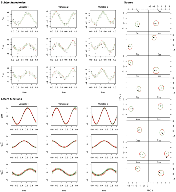
Figure D.8: MCMC and MFVB estimates for a problem with $p=3$ variables observed at an average of $15$ time points for $n=200$ subjects. Top left: estimated trajectories for a random subset of $3$ subjects, with the posterior mean (solid lines) and $95\%$ pointwise credible bands (dashed). The lines corresponding to MCMC (red) and MFVB (green) inference overlap. Bottom left: mean and eigenfunctions simulated (black) and estimated by MCMC inference (red) with $95\%$ credible bands (dashed) and by MFVB inference (green) for which estimates from $100$ replicates are overlaid. Right: scores simulated (black dots) and estimated by MCMC (posterior mean, red dots) inference and MFVB (posterior mean, green dots), with $95\%$ credible contours, for a random subset of $16$ subjects.

Figures D.9 and D.10 show a comparison of the errors on the estimated scores and latent functions for a grid of problems with $n\in\{50,100,200,300,400,500\}$, simulating $100$ replicates for each. The VMP, MFVB and MCMC errors are very similar, and all decrease as $n$ increases. Additionally, as we expect, when $n$ is small, the variability of the errors is greater (which is better seen for the scores, whose RMSE is presented on the original scale, rather than for the latent functions whose ISE is shown on the logarithmic scale).

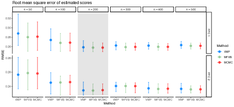
Figure D.9: Root mean square error (RMSE) of scores (FPC 1 first row, FPC 2 second row) for a problem with $p=3$ variables observed at an average of $15$ time points for a grid of $n\in\{50,100,200,300,400,500\}$ subjects, using VMP (blue), MFVB (green) and MCMC (red) inference. Each scenario is based on $100$ data replicates and the scenario shown on Figure 2 is shaded in grey.

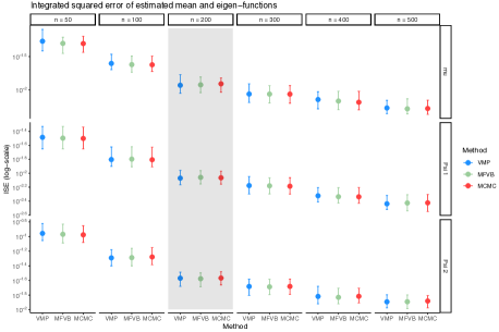
Figure D.10: Integrated squared error (ISE) of the mean function (first row) and two eigenfunctions (second and third rows) for a problem with $p=3$ variables observed at an average of $15$ time points for a grid of $n\leavevmode\nobreak\ \in\leavevmode\nobreak\ \{50,100,200,300,400,500\}$ subjects, using VMP (blue), MFVB (green) and MCMC (red) inference. Each scenario is based on $100$ data replicates and the scenario shown on Figure 2 is shaded in grey. For each replicate, per-variable ISE are computed and averaged across all $p$ variables.

D.2 Addendum on the comparison with frequentist multivariate FPCA

Figure D.11 compares the estimated scores with the true scores for one replicate of the setting where Happ and Greven (2018)’s method has the highest accuracy according to the simulation results of Section 5.3, namely, with $80$ observations per subject and variable, on average. The two methods perform similarly well; note that our approach permits quantifying the uncertainty around the scores thanks to posterior credible ellipses readily available from the estimated VMP posterior distributions.

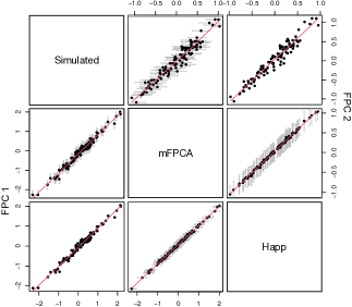
Figure D.11: Comparison of scores simulated and estimated with Happ’s and our approach for one data replicate of a problem with $80$ observations per subject and variable on average. The scores corresponding to the first (resp. second) eigenfunction are shown on the lower (resp. upper) diagonal part. $95\%$ credible intervals are shown for estimates obtained with our approach (grey); such uncertainty quantification is unavailable for Happ’s estimates.

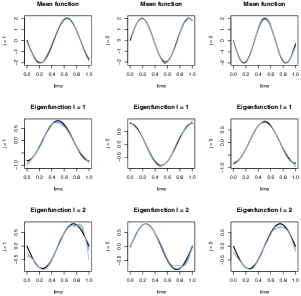
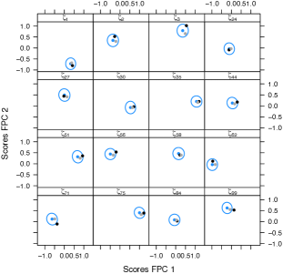
Figure D.12: Comparison of FPCA estimates obtained with Happ’s and our approaches, for a problem with $p=3$ variables, $n=100$ subjects, and an average of $80$ observations per variable and subject. Left: mean and eigen- functions simulated (black) and estimated by Happ’s (grey) and our (blue) approach. Right: scores simulated (black dots) and estimated by Happ’s approach (grey dots) and our approach (posterior mean, blue dots, and $95\%$ credible contours), for a random subset of $16$ subjects.

References

- Bergamaschi et al. (2021) L. Bergamaschi, F. Mescia, L. Turner, A. L. Hanson, P. Kotagiri, B. J. Dunmore, H. Ruffieux, A. De Sa, O. Huhn, M. D. Morgan, et al. Longitudinal analysis reveals that delayed bystander CD8+ T cell activation and early immune pathology distinguish severe COVID-19 from mild disease. Immunity, 54:1257–1275, 2021.
- Bishop (1999) C. M. Bishop. Variational pincipal components. In Proceedings of the Ninth International Conference on Artificial Neural Networks. Institute of Electrical and Electronics Engineers, 1999.
- Bishop (2006) C. M. Bishop. Pattern Recognition and Machine Learning. Springer, New York, 2006.
- Blei et al. (2017) D. M. Blei, A. Kucukelbir, and J. D. McAuliffe. Variational inference: A review for statisticians. Journal of the American Statistical Association, 112:859–877, 2017.
- Carpenter et al. (2017) B. Carpenter, A. Gelman, M. D. Hoffman, D. Lee, B. Goodrich, M. Betancourt, M. Brubaker, J. Guo, P. Li, and A. Riddell. Stan: A probabilistic programming language. Journal of Statistical Software, 76, 2017.
- Durbán et al. (2005) M. Durbán, J. Harezlak, M. P. Wand, and R. J. Carroll. Simple fitting of subject specific curves for longitudinal data. Statistics in Medicine, 24:1153–1167, 2005.
- Gelman (2006) A. Gelman. Prior distributions for variance parameters in hierarchical models (comment on article by Browne and Draper). Bayesian Analysis, 1:515–534, 2006.
- Gentle (2007) J. E. Gentle. Matrix Algebra. Springer, New York, 2007.
- Goldsmith et al. (2015) J. Goldsmith, V. Zippunnikov, and J. Schrack. Generalized multilevel function-on-scalar regression and principal component analysis. Biometrics, 71:344–353, 2015.
- Happ and Greven (2018) C. Happ and S. Greven. Multivariate functional principal component analysis for data observed on different (dimensional) domains. Journal of the American Statistical Association, 113:649–659, 2018.
- Holmes et al. (2021) E. Holmes, J. Wist, R. Masuda, S. Lodge, P. Nitschke, T. Kimhofer, R. L. Loo, S. Begum, B. Boughton, and R. Yang. Incomplete systemic recovery and metabolic phenoreversion in Post-Acute-Phase nonhospitalized COVID-19 Patients: Implications for assessment of Post-Acute COVID-19 syndrome. Journal of Proteome Research, 2021.
- James et al. (2000) G. M. James, T. J. Hastie, and C. A. Sugar. Principal component models for sparse functional data. Biometrika, 87:587–602, 2000.
- Li et al. (2020) C. Li, L. Xiao, and S. Luo. Fast covariance estimation for multivariate sparse functional data. Stat, 9:245–262, 2020.
- Lucas et al. (2020) C. Lucas, P. Wong, J. Klein, T. B. R. Castro, J. Silva, M. Sundaram, M. K. Ellingson, T. Mao, J. E. Oh, B. Israelow, et al. Longitudinal analyses reveal immunological misfiring in severe COVID-19. Nature, 584:463–469, 2020.
- Maestrini and Wand (2020) L. Maestrini and M. P. Wand. The Inverse G-Wishart distribution and variational message passing. arXiv e-prints, art. arXiv:2005.09876, 2020.
- Masuda et al. (2021) R. Masuda, S. Lodge, P. Nitschke, M. Spraul, H. Schaefer, S.-H. Bong, T. Kimhofer, D. Hall, R. L. Loo, Bizkarguenaga, C. Bruzzone, R. Gil-Redondo, N. Embade, J. M. Mato, E. Holmes, J. Wist, O. Millet, and J. K. Nicholson. Integrative modeling of plasma metabolic and lipoprotein biomarkers of SARS-CoV-2 infection in Spanish and Australian COVID-19 patient cohorts. Journal of Proteome Research, 20:4139–4152, 2021.
- Menictas and Wand (2013) M. Menictas and M. P. Wand. Variational inference for marginal longitudinal semiparametric regression. Stat, 2:61–71, 2013.
- Minka (2005) T. Minka. Divergence measures and message passing. Technical report, Microsoft Research Ltd., Cambridge, UK, 2005.
- Müller and Stadtmüller (2005) H. G. Müller and U. Stadtmüller. Generalised functional linear models. The Annals of Statistics, 33:774–805, 2005.
- Nolan et al. (2023) T. H. Nolan, J. Goldsmith, and D. Ruppert. Bayesian functional principal components analysis via variational message passing with multilevel extensions. Bayesian Analysis, 1(1):1–27, 2023.
- Ormerod and Wand (2010) J. T. Ormerod and M. P. Wand. Explaining variational approximations. The American Statistician, 64:140–153, 2010.
- Peluso et al. (2021) M. J. Peluso, S. Lu, A. F. Tang, M. S. Durstenfeld, H.-E. Ho, S. A. Goldberg, C. A. Forman, S. E. Munter, R. Hoh, and V. Tai. Markers of immune activation and inflammation in individuals with postacute sequelae of severe acute respiratory syndrome coronavirus 2 infection. The Journal of Infectious Diseases, 224:1839–1848, 2021.
- Ramsay and Silverman (2005) J. O. Ramsay and B. W. Silverman. Functional Data Analysis. Springer, New York, 2005.
- Ruffieux et al. (2023) Hélène Ruffieux, Aimee L Hanson, Samantha Lodge, Nathan G Lawler, Luke Whiley, Nicola Gray, Tui H Nolan, Laura Bergamaschi, Federica Mescia, Lorinda Turner, et al. A patient-centric modeling framework captures recovery from sars-cov-2 infection. Nature Immunology, 24(2):349–358, 2023.
- Ruppert (2002) D. Ruppert. Selecting the number of knots for penalized splines. Journal of Computational and Graphical Statistics, 11:735–757, 2002.
- Ruppert et al. (2003) D. Ruppert, M. P. Wand, and R. J. Carroll. Semiparametric Regression. Cambridge University Press, 2003.
- Ruppert et al. (2009) D. Ruppert, M. P. Wand, and R. J. Carroll. Semiparametric regression during 2003–2007. Electronic Journal of Statistics, 3:1193–1256, 2009.
- Tipping and Bishop (1999) M. E. Tipping and C. M. Bishop. Probabilistic principal component analysis. Journal of the Royal Statistical Society, Series B, 3:611–622, 1999.
- van der Linde (2008) A. van der Linde. Variational Bayesian functional PCA. Computational Statistics and Data Analysis, 53:517–533, 2008.
- Wand (2017) M. P. Wand. Fast approximate inference for arbitrarily large semiparametric regression models via message passing (with discussion). Journal of the American Statistical Association, 112:137–168, 2017.
- Wand and Ormerod (2008) M. P. Wand and J. T. Ormerod. On semiparametric regression with O’Sullivan penalized splines. Australian & New Zealand Journal of Statistics, 50:179–198, 2008.
- Wang et al. (2019) Y. Wang, G. Wang, L. Wang, and R. T. Ogden. Simultaneous confidence corridors for mean functions in functional data analysis of imaging data. Biometrics, 76:427–437, 2019.
- Yao et al. (2005) F. Yao, H. G. Müller, and J. L. Wang. Functional data analysis for sparse longitudinal data. Journal of the American Statistical Association, 100:577–590, 2005.
- Zou et al. (2016) H. Zou, N. Strawn, and D. B. Dunson. Bayesian graphical models for multivariate functional data. Journal of Machine Learning Research, pages 1–27, 2016.