Mixture of Weak & Strong Experts on Graphs

Abstract

Realistic graphs contain both rich self-features of nodes and informative structures of neighborhoods, jointly handled by a GNN in the typical setup. We propose to decouple the two modalities by mixture of weak and strong experts (Mowst), where the weak expert is a light-weight Multi-layer Perceptron (MLP), and the strong expert is an off-the-shelf Graph Neural Network (GNN). To adapt the experts’ collaboration to different target nodes, we propose a “confidence” mechanism based on the dispersion of the weak expert’s prediction logits. The strong expert is conditionally activated when either the node’s classification relies on neighborhood information, or the weak expert has low model quality. We reveal interesting training dynamics by analyzing the influence of the confidence function on loss: our training algorithm encourages the specialization of each expert by effectively generating soft splitting of the graph. In addition, our “confidence” design imposes a desirable bias toward the strong expert to benefit from GNN’s better generalization capability. Mowst is easy to optimize and achieves strong expressive power, with a computation cost comparable to a single GNN. Empirically, Mowst shows significant accuracy improvement on 6 standard node classification benchmarks (including both homophilous and heterophilous graphs).

1 Introduction

Graph Neural Networks (GNNs) have achieved tremendous success (Zhou et al., 2020; Wu et al., 2020). Many widely used models are derived based on the global properties of the graph. For example, Kipf & Welling (2016); Wu et al. (2019); Chen et al. (2020b) perform signal smoothing using the full Laplacian; Xu et al. (2019) tests $k$-hop isomorphism for all target nodes; Hamilton et al. (2017); Veličković et al. (2018) apply spatial aggregation on (approximation of) the full neighborhood. However, realistic graphs contain non-homogeneous patterns. Different parts of the graph may exhibit different characteristics. For example, locally homophilous and locally heterophilous regions may co-exist in one graph (Zhu et al., 2021). Suresh et al. (2021) further proposes a node-level assortativity metric to demonstrate the diverse signal mixing patterns across nodes. Zhang et al. (2021) notes that the number graph convolution iterations need to be adjusted on a per-node basis based on local structure. Therefore, a powerful model should have diversified treatments on different target nodes.

The root problem underlying the above challenge is the limited model capacity. One solution is to develop more advanced layer architectures to improve the expressiveness of a single GNN model (Yun et al., 2019; Brody et al., 2022; Zheng et al., 2023; Joshi et al., 2023). The other way is to combine existing GNN models into a Mixture-of-Experts (MoE) system (Jacobs et al., 1991; Hu et al., 2022), considering that MoE has effectively improved model capacity in many domains (Masoudnia & Ebrahimpour, 2014; Du et al., 2022; Lepikhin et al., 2021). However, both approaches have drawbacks. GNNs are both expensive to compute and hard to optimize. “Neighborhood explosion” (Chen et al., 2018) makes it infeasible to train a deep and complicated GNN model on commercial hardware. The widely observed oversmoothing (Chen et al., 2020a; Li et al., 2018) and oversquashing (Topping et al., 2022; Alon & Yahav, 2021) phenomena make it hard to optimize the model well. Therefore, the above two solutions increase model capacity at the cost of exacerbating the computation and optimization issues. Note that variants of MoE, exemplified by Sparse MoE (Shazeer et al., 2017), may partially address the computation challenge by activating only a subset of experts during inference. However, it is a well-known issue that the sparse gating may make the optimization even harder due to manually introduced discontinuity and intentionally added noises (Fedus et al., 2022).

To improve model capacity without significant trade-offs in computation overhead and optimization difficulty, we follow the basic MoE design philosophy, but take a step back to mix a simple Multi-Layer Perceptron (MLP) with an off-the-shelf GNN – an intentionally imbalanced combination unseen in traditional MoE models. The intuitive justifications are two-fold. First, the MLP and GNN models can specialize to address the two most fundamental modalities in realistic graphs: the feature of a node itself, and the structure of its neighborhood. The MLP, though much weaker than the GNN, can play an important role in various cases. For example, in a cluster of high homophily, the neighbors are similar, and thus aggregating their features via a GNN layer may not be more advantageous than extracting just the rich self-features of nodes. On the other hand, in the highly heterophilous parts of the graph, the edges connecting dissimilar neighbors may be noisy. Thus, performing message passing there may bring more harm than benefits (Zhu et al., 2020a). The MLP can help “clean up” the dataset for the GNN, enabling the strong expert to focus on the more complicated nodes whose neighborhood structure provides useful information for the learning task. The second justification for our “weak-strong” duo is that an MLP is both lightweight and easy to optimize. Its lack of recursive neighborhood aggregation not only makes the computation orders of magnitude cheaper than GNN (Wu et al., 2019; Zhang et al., 2022), but also automatically avoids oversmoothing and oversquashing.

Contributions.     We propose mixture of weak and strong experts (Mowst) on graphs, where the MLP and GNN experts specialize in the feature and structure modalities. To encourage collaboration without complicated gating functions, we propose a “confidence” mechanism to control the contribution of each expert on a per-node basis. Unlike recent MoE designs where experts are fused in each layer (Du et al., 2022; Lepikhin et al., 2021), our experts execute independently through their last layer and are then mixed based on a confidence score calculated by the dispersion of the MLP’s prediction logits. Our mixing mechanism has the following properties. First, since the confidence score solely depends on MLP’s output, the system is biased and inherently favors the GNN’s prediction. However, such bias is desirable since under the same training loss, a GNN can generalize better than an MLP (Yang et al., 2023). The extent of such bias depends on the confidence function, which can be learned in training. Second, our model-level (rather than layer-level) mixture makes the optimization easier and more explainable. Through theoretical analysis of the optimization behavior, we uncover various interesting collaboration modes between the two experts. During training, the system dynamically creates a soft splitting of the graph based on not only the nodes’ characteristics but also the two experts’ relative model quality. Such splitting leads to experts’ specialization. Upon convergence, it is possible that the GNN expert dominates and the splitting becomes insignificant. Even so, Mowst still outperforms a GNN alone: the MLP denoises for the GNN during training, ultimately enabling the GNN to converge better. The above advantages of Mowst, together with the theoretically high expressive power, come at the cost of minor computation overhead. In experiments, we extensively evaluate Mowst on 2 types of GNN experts and 6 standard benchmarks covering both homophilous and heterophilous graphs. We show consistent accuracy improvements over state-of-the-art baselines.

2 Model

Algorithm 1 Mowst inference

Input: $\IfEq{}{}{\mathcal{G}}{\mathcal{G}}\left(\IfEq{}{}{\mathcal{V}}{\mathcal{V}},\IfEq{}{}{\mathcal{E}}{\mathcal{E}},\IfEq{}{}{\bm{X}}{\bm{X}^{\left(\right)}}\right)$; target node $v$

Output: prediction of $v$

Run the MLP expert on $v$

Get prediction $\bm{p}_{v}$ & confidence $C\left(\bm{p}_{v}\right)\in[0,1]$

if random number $q\in[0,1]$ has $q<C\left(\bm{p}_{v}\right)$ then

     Predict $v$ by MLP’s prediction $\bm{p}_{v}$

else

     Run the GNN expert on $v$

     Predict $v$ by GNN’s prediction $\bm{p}^{\prime}_{v}$

end if

Algorithm 2 Mowst training

Input: $\IfEq{}{}{\mathcal{G}}{\mathcal{G}}\left(\IfEq{}{}{\mathcal{V}}{\mathcal{V}},\IfEq{}{}{\mathcal{E}}{\mathcal{E}},\IfEq{}{}{\bm{X}}{\bm{X}^{\left(\right)}}\right)$; training labels $\{\bm{y}_{v}\}$

Initialize MLP & GNN weights as $\bm{\theta}_{0}$ & $\bm{\theta}^{\prime}_{0}$

for round $r=1$ until convergence do

     Fix GNN weights $\bm{\theta}^{\prime}_{r-1}$

     Update MLP weights to $\bm{\theta}_{r}$ by gradient descent on $L$ until convergence

     Fix MLP weights $\bm{\theta}_{r}$

     Update GNN weights to $\bm{\theta}^{\prime}_{r}$ by gradient descent on $L$ until convergence

end for

Our discussion mainly focuses on the most fundamental form, consisting of a weak MLP expert and a strong GNN expert (§2.7 presents the generalization to more experts). The key challenge lies in designing the mixture module in consideration of the inherent imbalance between experts. There are subtleties in experts’ interactions. On the one hand, the weak expert should only be cautiously activated to avoid accuracy degradation. On the other hand, for nodes that can be truly mastered by the MLP, we should ensure that the weak expert can meaningfully contribute rather than being overshadowed by its stronger counterpart. We present the overall model in §2.1 and §2.2, and discuss how our mixing mechanism encourages collaboration via theory §2.3 and analysis §2.4. We also present a variant of Mowst in §2.5, and analyze the expressive power and computation cost in §2.6.

Notations.     Let $\IfEq{}{}{\mathcal{G}}{\mathcal{G}}\left(\IfEq{}{}{\mathcal{V}}{\mathcal{V}},\IfEq{}{}{\mathcal{E}}{\mathcal{E}},\IfEq{}{}{\bm{X}}{\bm{X}^{\left(\right)}}\right)$ be a graph with node set $\IfEq{}{}{\mathcal{V}}{\mathcal{V}}$ and edge set $\IfEq{}{}{\mathcal{E}}{\mathcal{E}}$. Each node $v$ has a length-$f$ raw feature vector $\bm{x}_{v}$. The node features can be stacked as $\IfEq{}{}{\bm{X}}{\bm{X}^{\left(\right)}}\in\mathbb{R}^{\left\lvert\IfEq{}{}{\mathcal{V}}{\mathcal{V}}\right\rvert\times f}$. Denote $v$’s ground truth label as $\bm{y}_{v}\in\mathbb{R}^{n}$, where $n$ is the number of classes. Denote the model prediction as $\bm{p}_{v}\in\mathbb{R}^{n}$.

2.1 Mowst

Inference.     By Algorithm 1, on a target $v$, the two experts each execute independently until they generate their own predictions $\bm{p}_{v}$ and $\bm{p}_{v}^{\prime}$. The mixture module either accepts $\bm{p}_{v}$ with probability $C\left(\bm{p}_{v}\right)$ (in which case we do not need to execute the GNN at all), or discards $\bm{p}_{v}$ and uses $\bm{p}_{v}^{\prime}$ as the final prediction. The score $C\left(\bm{p}_{v}\right)$ reflects how confident the MLP is in its prediction. e.g., in binary classification, $\bm{p}_{v}=[0,1]^{\mathsf{T}}$ and $[0.5,0.5]^{\mathsf{T}}$ correspond to cases where the MLP is certain and uncertain about its prediction. The corresponding $C\left(\bm{p}_{v}\right)$ should be close to 1 and 0 respectively.

Training.     The training (Algorithm 2) minimizes the expected loss of inference. Thus, the loss is:

$$L_{\text{{Mowst}}}= \frac{1}{\left\lvert\IfEq{}{}{\mathcal{V}}{\mathcal{V}}\right\rvert}\sum_{v\in\IfEq{}{}{\mathcal{V}}{\mathcal{V}}}\big{(}C\left(\bm{p}_{v}\right)\cdot L\left(\bm{p}_{v},\bm{y}_{v}\right)+\left(1-C\left(\bm{p}_{v}\right)\right)\cdot L\left(\bm{p}^{\prime}_{v},\bm{y}_{v}\right)\big{)}$$ (1)

where $\bm{p}_{v}={\text{MLP}\left(\bm{x}_{v};\bm{\theta}\right)}$ and $\bm{p}^{\prime}_{v}={\text{GNN}\left(\bm{x}_{v};\bm{\theta}^{\prime}\right)}$ are the experts’ predictions; $\bm{\theta}$ and $\bm{\theta}^{\prime}$ are the experts’ model parameters. $L_{\text{{Mowst}}}$ is fully differentiable. While we could simultaneously optimize both experts via standard gradient descent, Algorithm 2 shows an alternative “training in turn” strategy: we fix one expert’s parameters while optimizing the other. Training in turn enables the experts to more thoroughly optimize themselves despite the different convergence behaviors due to the different model architectures. If $C$ is learnable (see §2.2), we update its parameters together with MLP’s $\bm{\theta}$.

Intuition.     We demonstrate via a simple case study how $C$ moderates the two experts. Suppose at some point of training, the two experts have the same loss on some $v$. In case 1, $v$’s self features are sufficient for a good prediction, then MLP can make $\bm{p}_{v}$ more certain to lower its $L\left(\bm{p}_{v},\bm{y}_{v}\right)$ and increase $C$. The better MLP’s loss then contributes more to $L_{\text{{Mowst}}}$ than GNN’s loss, thus improving the overall $L_{\text{{Mowst}}}$. In case 2, $v$’s self-features are insufficient for further reducing MLP’s loss. Then if the MLP makes $\bm{p}_{v}$ more certain, $L_{\text{{Mowst}}}$ will deteriorate since an increased $C$ will up-weight the contribution of a worse $L\left(\bm{p}_{v},\bm{y}_{v}\right)$. Otherwise, if the MLP acts in the reverse way to even degrade $\bm{p}_{v}$ to random guess, $L\left(\bm{p}_{v},\bm{y}_{v}\right)$ will still be worse but $C$ will also reduce to 0. Thus, $L_{\text{{Mowst}}}$ remains unaffected even if MLP is completely ignored. Case 2 shows the bias of Mowst towards the GNN, but thanks to case 1, the weak MLP can indeed play a role on nodes where it specializes well.

2.2 Confidence function

In this sub-section, we omit subscript $v$. We formally categorize the class of the confidence function $C$. Consider single task, multi-class node prediction, where $n$ is the total number of classes. The input to $C$, $\bm{p}$, belongs to the standard $\left(n-1\right)$-simplex, $\IfEq{n-1}{}{\mathcal{S}}{\mathcal{S}}_{n-1}$. i.e., $\sum_{1\leq i\leq n}p_{i}=1$ and $p_{i}\geq 0$, for $i=1,\ldots,n$. The output of $C$ falls between 0 and 1. Since $C$ depends on how certain the MLP’s prediction is, we further apply decomposition as $C=G\circ D$, where $D$ takes $\bm{p}$ as input and computes its dispersion, and $G$ is a real-valued scalar function. We formally define $G$ and $D$ as follows:

Definition 2.1.

$D:\IfEq{n-1}{}{\mathcal{S}}{\mathcal{S}}_{n-1}\mapsto\mathbb{R}$ is continuous and quasiconvex where $D\left(\frac{1}{n}\bm{1}\right)=0$ and $D\left(\bm{p}\right)>0$ if $\bm{p}\neq\frac{1}{n}\bm{1}$. $G:\mathbb{R}\mapsto\mathbb{R}$ is monotonically non-decreasing where $G\left(0\right)=0$ and $0<G\left(x\right)\leq 1,\forall x>0$.

Proposition 2.2.

$C=G\circ D$ is quasiconvex.

$D$’s definition states that only a prediction as bad as a random guess receives 0 dispersion. Typical dispersion functions such as variance and (offsetted) negative entropy belong to our class of $D$. $G$’s definition states that the confidence $C$ does not decrease with a higher dispersion, which is reasonable as dispersion reflects the certainty of the prediction. During training, we can fix $C$ by manually specifying both $D$ and $G$. Alternatively, we can use a lightweight neural network (e.g., MLP) to learn $G$, where the input to $G$’s MLP is the variance and negative entropy computed by $D$ (§4).

2.3 Interaction Between Experts

On any node, the experts’ coefficients, $C$ and $1-C$, always sum up to 1. When training starts, the experts compete for higher weight. When training progresses, the experts specialize in diverse ways. Correspondingly, $C$ evolves to accumulate on some nodes, while diminish on the others. The eventual $C$ distribution turns experts’ competition into collaboration, improving the overall Mowst accuracy.

Assume the MLP expert can fit an arbitrary function on node features. This is reasonable as an MLP is a universal approximator (Hornik et al., 1989) and optimizing it is easy. Accordingly, we divide the graph nodes into $m$ disjoint groups, where nodes are in the same group, $\IfEq{i}{}{\mathcal{M}}{\mathcal{M}}_{i}$, if and only if they have indistinguishable self-features. For all nodes in $\IfEq{i}{}{\mathcal{M}}{\mathcal{M}}_{i}$, an MLP generates the same prediction denoted as $\hat{\bm{p}}_{i}$. However, nodes $u,v\in\IfEq{i}{}{\mathcal{M}}{\mathcal{M}}_{i}$ may have different labels $\bm{y}_{u}\neq\bm{y}_{v}$. In such a case, the MLP expert can never distinguish $u$ from $v$ since neighborhood information is necessary. Let $\bm{\alpha}_{i}$ be the label distribution for $\IfEq{i}{}{\mathcal{M}}{\mathcal{M}}_{i}$. i.e., $\alpha_{ij}\in(0,1)$ portion of nodes in $\IfEq{i}{}{\mathcal{M}}{\mathcal{M}}_{i}$ have label $j$, and $\sum_{1\leq j\leq n}\alpha_{ij}=1$. Consider the phase of training the MLP expert while fixing the GNN. We analyze the optimal $\hat{\bm{p}}^{*}_{i}$ that minimizes $L_{\text{{Mowst}}}$ in Equation 1. The optimization problem is as follows (Appendix C.1):

$$\{\hat{\bm{p}}_{i}^{*}\}=\arg\min_{\{\hat{\bm{p}}_{i}\}}L_{\text{{Mowst}}}=\arg\min_{\{\hat{\bm{p}}_{i}\}}\sum_{1\leq i\leq m}C\left(\hat{\bm{p}}_{i}\right)\cdot\left(\hat{L}_{\bm{\alpha}_{i}}\left(\hat{\bm{p}}_{i}\right)-\mu_{i}\right)$$ (2)

where $\hat{L}_{\bm{\alpha}_{i}}\left(\hat{\bm{p}}_{i}\right)=\frac{1}{\left\lvert\IfEq{i}{}{\mathcal{M}}{\mathcal{M}}_{i}\right\rvert}\sum_{v\in\IfEq{i}{}{\mathcal{M}}{\mathcal{M}}_{i}}L\left(\hat{\bm{p}}_{i},\bm{y}_{v}\right)=-\sum_{1\leq j\leq n}\alpha_{ij}\cdot\log\hat{p}_{ij}$ is the average MLP cross-entropy loss on nodes in $\IfEq{i}{}{\mathcal{M}}{\mathcal{M}}_{i}$; $\mu_{i}=\frac{1}{\left\lvert\IfEq{i}{}{\mathcal{M}}{\mathcal{M}}_{i}\right\rvert}\sum_{v\in\IfEq{i}{}{\mathcal{M}}{\mathcal{M}}_{i}}L\left(\bm{p}^{\prime}_{v},\bm{y}_{v}\right)$ is a constant representing the average GNN loss on nodes in $\IfEq{i}{}{\mathcal{M}}{\mathcal{M}}_{i}$. We first summarize the properties of the loss as follows.

Proposition 2.3.

Given $\bm{\alpha}_{i}$, $\hat{L}_{\bm{\alpha}_{i}}\left(\hat{\bm{p}}_{i}\right)$ is a convex function of $\hat{\bm{p}}_{i}$ with unique minimizer $\hat{\bm{p}}_{i}^{*}=\bm{\alpha}_{i}$. Let $\Delta\left(\bm{\alpha}\right)=\hat{L}_{\bm{\alpha}}\left(\bm{\alpha}\right)$ be a function of $\bm{\alpha}$, $\Delta$ is a concave function with unique maximizer $\bm{\alpha}^{*}=\frac{1}{n}\bm{1}$.

$\Delta\left(\bm{\alpha}_{i}\right)$ reflects the best possible performance of any MLP on a group $\mathcal{M}_{i}$. We now analyze the optimization problem 2. Theorem 2.4 quantifies the positions of the minimizer $\hat{\bm{p}}_{i}^{*}$ and the corresponding values of $C$. In case 3 ($\Delta\left(\bm{\alpha}_{i}\right)<\mu_{i}$), it is impossible to derive the exact $\hat{\bm{p}}_{i}^{*}$ without knowing the specific $C$. Therefore, we bound $\hat{\bm{p}}^{*}_{i}$ via “sub-level sets”, which characterize the shapes of the loss and confidence functions. The last sentence of Theorem 2.4 shows the “tightness” of the bound.

Theorem 2.4.

Suppose $C=G\circ D$ follows Definition 2.1. Denote $\mathcal{L}_{\bm{\alpha}_{i}}^{\mu_{i}}=\{\hat{\bm{p}}_{i}\;|\;\hat{L}_{\bm{\alpha}_{i}}\left(\hat{\bm{p}}_{i}\right)=\mu_{i}\}$ and $\mathcal{L}_{\bm{\alpha}_{i}}^{<\mu_{i}}=\{\hat{\bm{p}}_{i}\;|\;\hat{L}_{\bm{\alpha}_{i}}\left(\hat{\bm{p}}_{i}\right)<\mu_{i}\}$ as the level set and strict sublevel set of $\hat{L}_{\bm{\alpha}_{i}}$. Denote $\mathcal{C}^{<\mu_{i}}=\{\hat{\bm{p}}_{i}\;|\;C\left(\hat{\bm{p}}_{i}\right)<\mu_{i}\}$ as the strict sublevel set of $C$. For a given $\bm{\alpha}_{i}\neq\frac{1}{n}\bm{1}_{n}$, the minimizer $\hat{\bm{p}}_{i}^{*}$ satisfies:

• If $\Delta\left(\bm{\alpha}_{i}\right)>\mu_{i}$, then $\hat{\bm{p}}_{i}^{*}=\frac{1}{n}\bm{1}_{n}$ and $C\left(\hat{\bm{p}}_{i}^{*}\right)=0$.

• If $\Delta\left(\bm{\alpha}_{i}\right)=\mu_{i}$, then $\hat{\bm{p}}_{i}^{*}=\bm{\alpha}_{i}$ or $\hat{\bm{p}}_{i}^{*}=\frac{1}{n}\bm{1}$.

• If $\Delta\left(\bm{\alpha}_{i}\right)<\mu_{i}$, then $\hat{\bm{p}}_{i}^{*}\in\mathcal{L}_{\bm{\alpha}_{i}}^{<\mu_{i}}-\mathcal{C}^{<\mu^{\prime}}$ where $\mu^{\prime}=C\left(\bm{\alpha}_{i}\right)\leq C\left(\hat{\bm{p}}_{i}^{*}\right)\leq G\left(\max_{\hat{\bm{p}}_{i}\in\mathcal{L}_{\bm{\alpha}_{i}}^{\mu_{i}}}D\left(\hat{\bm{p}}_{i}\right)\right)$. Further, there exists $C$ such that $\hat{\bm{p}}_{i}^{*}=\bm{\alpha}_{i}$, or $\hat{\bm{p}}_{i}^{*}$ is sufficiently close to the level set $\mathcal{L}_{\bm{\alpha}_{i}}^{\mu_{i}}$.

Corollary 2.4.1.

For binary classification ($n=2$), w.l.o.g, assume $\alpha_{i1}\in[0.5,1)$. Define $\hat{L}_{i+}\left(p\right)=\hat{L}_{\bm{\alpha}}\left([p,1-p]^{\mathsf{T}}\right)$ for $p\in[\alpha_{i1},1)$. For strictly quasiconvex $D$ and monotonically increasing $G$, $\hat{p}_{i1}^{*}\in\left[\alpha_{i1},\hat{L}_{i+}^{-1}\left(\mu_{i}\right)\right)$ and $C\left(\bm{\alpha}_{i}\right)\leq C\left(\hat{\bm{p}}_{i}^{*}\right)<C\left(\left[\hat{L}_{i+}^{-1}\left(\mu_{i}\right),1-\hat{L}_{i+}^{-1}\left(\mu_{i}\right)\right]^{\mathsf{T}}\right)$ when $\Delta\left(\bm{\alpha}_{i}\right)<\mu_{i}$.

Proposition 2.3 and Theorem 2.4 jointly reveal factors affecting the MLP’s contribution to the overall system: 1. Ratio of indistinguishable nodes, $\bm{\alpha}_{i}$: the closer $\bm{\alpha}_{i}$ is to $\frac{1}{n}\bm{1}$, the harder it is to reduce the MLP loss, and thus the lower the confidence $C$ is. 2. Relative strength of experts, $\Delta\left(\bm{\alpha}_{i}\right)-\mu_{i}$: when the best possible MLP loss $\Delta\left(\bm{\alpha}_{i}\right)$ cannot beat the GNN loss $\mu_{i}$, the MLP simply learns to give up on the node group $\mathcal{M}_{i}$ by generating random guess $\hat{\bm{p}}_{i}^{*}=\frac{1}{n}\bm{1}$. Otherwise, if the MLP can possibly outperform GNN, it will do so by learning a $\hat{\bm{p}}_{i}^{*}$ in some neighborhood of $\bm{\alpha}_{i}$ and obtaining positive confidence $C$. The worse the GNN (i.e., larger $\mu_{i}$), the easier to obtain a more dispersed $\hat{\bm{p}}_{i}^{*}$ (i.e., enlarged $\mathcal{L}_{\bm{\alpha}_{i}}^{<\mu_{i}}$), and so the easier to achieve a larger $C$ (i.e., increased $\max_{\hat{\bm{p}}_{i}\in\mathcal{L}_{\bm{\alpha}_{i}}^{\mu_{i}}}D\left(\hat{\bm{p}}_{i}\right)$). 3. Shape of the confidence function$C$: the sub-level set, $\mathcal{C}^{<\mu^{\prime}}$, constrains the range of $\hat{\bm{p}}_{i}^{*}$. Additionally, changing $G$’s shape can push $C\left(\hat{\bm{p}}_{i}^{*}\right)$ towards the lower bound $C\left(\bm{\alpha}_{i}\right)$ or the upper bound $G\left(\max_{\hat{\bm{p}}_{i}\in\mathcal{L}_{\bm{\alpha}_{i}}^{\mu_{i}}}D\left(\hat{\bm{p}}_{i}\right)\right)$. See Appendix B.1 for specific $G$ constructions and all proofs.

Point (1) above shows a property of the graph. Point (2) leads to diverse training dynamics (§2.4). In addition, it reflects the inherent bias of Mowst: a better GNN completely dominates the MLP by $1-C\left(\hat{\bm{p}}_{i}^{*}\right)=1$, while a better MLP only softly deprecates the GNN with $C\left(\hat{\bm{p}}_{i}^{*}\right)<1$. Such bias is by design: first, a GNN is harder to optimize than an MLP. So even if it temporarily performs badly during training, we still preserve positive $1-C$ so that it has a chance to later catch up with the MLP. Second, since a GNN can generalize better on the test set (Yang et al., 2023), we prefer it when the training performance of the two experts is similar. Point (3) justifies our learnable $G$ design in §2.2.

2.4 Training dynamics

Specialization via data splitting.     At the beginning of training ($r=1$, Algorithm 2), a randomly initialized GNN approximately produces random guess. So MLP generates a distribution of $C$ over all training nodes purely based on self-feature importance. Denote the subset of nodes with large $1-C$ as $\mathcal{S}_{\text{GNN}}$. When it is GNN’s turn to update its model parameters, the GNN optimizes $\mathcal{S}_{\text{GNN}}$ better due to the larger loss weight. In the next round $r=2$, the MLP will fail to beat the GNN on many nodes, especially on $\mathcal{S}_{\text{GNN}}$. According to Theorem 2.4, the MLP will completely ignore such challenging nodes (by setting $C=0$ on $\mathcal{S}_{\text{GNN}}$), simplifying the learning task for the weak expert. When MLP again converges, it specializes better on a smaller subset of the training set, and the updated $C$ distribution makes the data partition between the two experts more clear. This process goes on and each additional round of “in-turn training” reinforces better specialization between experts.

Denoised fine-tuning.     From analysis above, it is natural to expect that MLP is assigned with a significant portion of nodes when the overall Mowst training converges. Yet we empirically observe that this is not always the case. When the GNN is really powerful, it can possibly dominate MLP on almost all nodes. This seems to degrade Mowst to a vanilla GNN during inference when MLP plays a negligible role. Surprisingly, Mowst still achieves significant accuracy improvement. We next uncover how MLP helps us fine-tune a better GNN by denoising a small number of critical nodes during training. Imagine 3 categories of nodes: 1. $\IfEq{1}{}{\mathcal{S}}{\mathcal{S}}_{1}$(e.g., 95% of $\IfEq{}{}{\mathcal{V}}{\mathcal{V}}$), where GNN has converged very well, 2. $\IfEq{2}{}{\mathcal{S}}{\mathcal{S}}_{2}$(e.g., 4% of $\IfEq{}{}{\mathcal{V}}{\mathcal{V}}$), where GNN can potentially further improve, 3. $\IfEq{3}{}{\mathcal{S}}{\mathcal{S}}_{3}$(e.g., 1% of $\IfEq{}{}{\mathcal{V}}{\mathcal{V}}$), where GNN performs badly due to unrecoverable noises. A standalone GNN may be stuck in sub-optimality since the harmful gradients from $\IfEq{3}{}{\mathcal{S}}{\mathcal{S}}_{3}$ may counter-act the useful gradients from $\IfEq{2}{}{\mathcal{S}}{\mathcal{S}}_{2}$. To improve GNN on $\IfEq{2}{}{\mathcal{S}}{\mathcal{S}}_{2}$, the MLP expert needs to break the equilibrium. From the §2.3 analysis on experts’ relative strength, MLP will have $C=0$ on $\IfEq{1}{}{\mathcal{S}}{\mathcal{S}}_{1}$, low $C$ on $\IfEq{2}{}{\mathcal{S}}{\mathcal{S}}_{2}$ and high $C$ on $\IfEq{3}{}{\mathcal{S}}{\mathcal{S}}_{3}$. Essentially, MLP ignores most of $\IfEq{}{}{\mathcal{V}}{\mathcal{V}}$ and overfits the small set of $\IfEq{3}{}{\mathcal{S}}{\mathcal{S}}_{3}$. MLP’s overfitting eliminates the harmful gradients for the GNN, enabling it to fine-tune on $\IfEq{2}{}{\mathcal{S}}{\mathcal{S}}_{2}$. In this case, MLP is a training-time noise filter.

2.5 Mowst^$\star$

We propose a model variant, Mowst^$\star$, by modifying the training loss of Mowst. In Equation 1, we compute the losses of the two experts separately, and then combine them via $C$ to get the overall loss $L_{\text{{Mowst}}}$. In Equation 3, we first use $C$ to combine the predictions of the two experts, $\bm{p}_{v}$ and $\bm{p}_{v}^{\prime}$, and then calculate a single loss for $L_{\text{{Mowst}}}^{\star}$. Note that the cross entropy loss, $L\left(\cdot,\bm{y}_{v}\right)$ is convex, and the weighted sum based on $C$ also corresponds to a convex combination. We thus derive Proposition 2.5, which states that Mowst^$\star$ is theoretically better than Mowst due to a lower loss.

$$L_{\text{{Mowst}}}^{\star}=\frac{1}{\left\lvert\IfEq{}{}{\mathcal{V}}{\mathcal{V}}\right\rvert}\sum_{v\in\IfEq{}{}{\mathcal{V}}{\mathcal{V}}}L\big{(}C\left(\bm{p}_{v}\right)\cdot\bm{p}_{v}+\left(1-C\left(\bm{p}_{v}\right)\right)\cdot\bm{p}^{\prime}_{v},\;\bm{y}_{v}\big{)}$$ (3)

Proposition 2.5.

$L_{\text{{Mowst}}}$ upper-bounds $L_{\text{{Mowst}}}^{\star}$.

Since Mowst^$\star$ only has a single loss term, we no longer use “in-turn training” of Algorithm 2. Instead, we directly differentiate $L_{\text{{Mowst}}}^{\star}$ and update the MLP, GNN and the learnable $C$ altogether. During inference, Mowst^$\star$ computes both experts and predicts via $C\left(\bm{p}_{v}\right)\cdot\bm{p}_{v}+\left(1-C\left(\bm{p}_{v}\right)\right)\cdot\bm{p}_{v}^{\prime}$.

Mowst vs. Mowst^$\star$.     Both variants have similar collaboration behaviors (e.g., §2.4), fundamentally determined by the “weak-strong” design choice and the confidence mechanism. Regarding tradeoffs, Mowst may be easier to optimize as its “in-turn training” fully decouples the experts’ different model architectures, while Mowst^$\star$ enjoys a theoretically lower loss. Both variants can be practically useful.

2.6 Expressive power and computation complexity

We jointly analyze Mowst and Mowst^$\star$ due to their commonalities. Since the MLP and GNN experts execute all their layers independently before mixture, it is intuitive that our system can express a vanilla single-expert model by simply disabling the other expert. In Proposition 2.6, we construct a specific $G$ so that the confidence function acts like a binary gate between experts. Theorem 2.7 provides a stronger result on the GCN architecture (Kipf & Welling, 2016). The idea (Appendix B.3.1) is that, when neighbors are noisy (or even adversarial), their aggregation brings more harm than benefit. An MLP is a simple yet effective way to eliminate such neighbor noises. The theoretical proof is inherently consistent with the empirically observed “denoising” behavior discussed in §2.4.

Proposition 2.6.

Mowst and Mowst^$\star$ are at least as expressive as the MLP or GNN expert alone.

Theorem 2.7.

Mowst-GCN and Mowst^$\star$-GCN are more expressive than the GCN expert alone.

For computation complexity, we consider the average cost of predicting one node in inference. For sake of discussion, we consider the GCN architecture and assume that both experts have the same number of layers $\ell$ and feature dimension $f$. In the worst case, both experts are activated (note from Algorithm 1 that we can skip the strong expert with probability $C$). The cost of the GCN is lower bound by $\Omega\left(f^{2}\cdot\left(\ell+b_{\ell-1}\right)\right)$ where $b_{\ell-1}$ is the average number of $\left(\ell-1\right)$-hop neighbors. The cost of the MLP is $O\left(f^{2}\cdot\ell\right)$. On large graphs, the neighborhood size $b_{\ell-1}$ can grow exponentially with $\ell$. So realistically, $b_{\ell-1}\gg\ell$. This means the worst-case cost of Mowst or Mowst^$\star$ is similar to that of a vanilla GCN. The conclusion still holds if we use an additional, lightweight MLP to compute the confidence score $C$ (such an MLP only approximates a scalar function $G$, and thus is very compact).

2.7 Mixture of progressively stronger experts

Suppose we have a series of $k$ progressively stronger experts where expert $i$ is stronger than $j$ if $i>j$ (e.g., 3 experts consisting of MLP, SGC (Wu et al., 2019) and GCN (Kipf & Welling, 2016)). Mowst and Mowst^$\star$ can be generalized following a recursive formulation. Let $L_{i}^{v}$ be the loss of expert $i$ on node $v$, $L_{\geq i}^{v}$ be the loss of a Mowst sub-system consisting of experts $i$ to $k$, and $C^{v}_{i}$ be the confidence of expert $i$ computed by $i$’s prediction on node $v$. Then Equation 1 generalizes to $L_{\text{{Mowst}}}=\frac{1}{\left\lvert\IfEq{}{}{\mathcal{V}}{\mathcal{V}}\right\rvert}\sum_{v\in\IfEq{}{}{\mathcal{V}}{\mathcal{V}}}L_{\geq 1}^{v}$ and $L_{\geq i}^{v}=C_{i}^{v}\cdot L_{i}^{v}+\left(1-C_{i}^{v}\right)\cdot L_{\geq i+1}^{v}$. During inference, similar to Algorithm 1, the strong expert will be activated only when all previous weaker experts are passed due to their low confidence. The case for Mowst^$\star$ can be derived similarly. See Appendix C.2 for final form of $L_{\text{{Mowst}}}$. Due to the recursive way of adding new experts, all our analysis and observation in previous sections still hold. For example, the expressive power is ensured as follows:

Proposition 2.8.

Mowst and Mowst^$\star$ are at least as expressive as any expert alone.

3 Related Work

Mixture-of-Experts.     Since its original proposal (Jacobs et al., 1991), MoE has been effective in increasing model capacity (Masoudnia & Ebrahimpour, 2014; Yuksel et al., 2012; Riquelme et al., 2021). The key idea is to localize / specialize different expert models to different partitions of the data. Typically, experts have comparable strengths. Thus, the numerous gating functions in the literature have a symmetric form w.r.t. all experts without biasing towards any specific one (e.g., variants of softmax (Jordan & Jacobs, 1994; Shazeer et al., 2017; Puigcerver et al., 2023)). In comparison, Mowst deliberately breaks the balance among experts and adopts a biased gating. Another major concern in existing MoE models is the increased computation cost. Sparse gating is needed to save computation by conditionally deactivating some experts. However, it is widely observed that such sparsity causes training instability (Fedus et al., 2022; Shazeer et al., 2017; Puigcerver et al., 2023). Under our confidence-based gating, Mowst is both easy to train (§2.4) and computationally efficient (§2.6). Finally, many recent designs apply MoE in each layer of a large model (Riquelme et al., 2021; Du et al., 2022; Lepikhin et al., 2021), while Mowst only mixes at the output layers. We fully decouple the experts with imbalanced strengths in consideration of their different training dynamics.

MoE & model ensemble on graphs.     GraphDIVE (Hu et al., 2022) proposed mixture of multi-view experts to address the class-imbalance issue in graph classification. GraphMoE (Wang et al., 2023) proposed to mix multiple GNN experts via the top-$K$ sparse gating (Shazeer et al., 2017). Zhou & Luo (2019) explored a similar idea of mixing multiple GNNs with existing gating functions. AdaGCN (Sun et al., 2021) proposed a model ensemble technique for GNNs, based on the classic AdaBoost algorithm (Freund et al., 1999). In addition, AM-GCN (Wang et al., 2020) performs graph convolution on the decoupled topological and feature graphs to learn multi-channel information.

Decoupling feature & structure information.     GraphSAGE (Hamilton et al., 2017), GCNII (Chen et al., 2020b) and H₂GCN (Zhu et al., 2020b) use various forms of residual connections to facilitate self-feature propagation. GPR-GNN (Chien et al., 2021), MixHop (Abu-El-Haija et al., 2019) and SIGN (Frasca et al., 2020) blend information from various hops away via different weighting strategies. NDLS (Zhang et al., 2021) performs adaptive $k$-hop sampling to customize the per-node receptive field. GLNN (Zhang et al., 2022) distills structural information into an MLP. These methods implicitly decouple the feature and structure information implicitly within one model, while Mowst does so explicitly via separate expert models. The above models can also be a GNN expert of Mowst.

4 Experiments

We use the notation “Mowst(^$\star$)” when we do not differentiate Mowst (§2.1) and Mowst^$\star$ (§2.5).

Setup.     We evaluate Mowst(^$\star$) on a diverse set of benchmarks, including 3 homophilous graphs (Flickr (Zeng et al., 2020), ogbn-arxiv and ogbn-products (Hu et al., 2020)) and 3 heterophilous graphs (Penn94, pokec and twitch-gamer (Lim et al., 2021)). Following the literature, we perform node prediction with the “accuracy” metric, under standard training / validation / test split. The graph sizes range from 89K (Flickr) to 2.4M (ogbn-products) nodes. See details in Appendix A.1.

Baselines.     GCN (Kipf & Welling, 2016), GraphSAGE (Hamilton et al., 2017), GAT (Veličković et al., 2018) and GIN (Xu et al., 2019) are the most widely used GNN architectures achieving, state-of-the-art accuracy on both homophilous (Hu et al., 2020; Shi et al., 2023) and heterophilous (Lim et al., 2021; Zhu et al., 2021; Platonov et al., 2023) graphs. In addition, GPR-GNN (Chien et al., 2021) decouples the aggregation of neighbors within different hops, achieving flexibility in learning feature and structure information. AdaGCN (Sun et al., 2021) and GraphMoE (Wang et al., 2023) are the state-of-the-art ensemble and MoE models respectively, both combining multiple GNNs.

Hyperparameters.     For Flickr, ogbn-products and ogbn-arxiv, we follow the original literature (Hu et al., 2020; Zeng et al., 2021) to set the number of layers as 3 and hidden dimension as 256, for all the baselines as well as for both the MLP and GNN experts of Mowst(^$\star$). Regarding Penn94, pokec and twitch-gamer, the authors of the original paper (Lim et al., 2021) searched for the best network architecture for each baseline independently. We follow the same protocol and hyperparameter space for our baselines and Mowst(^$\star$). We set an additional constraint on Mowst(^$\star$) to ensure fair comparison under similar computation costs: we first follow Lim et al. (2021) to determine the number of layers $\ell$ and hidden dimension $d$ of the baseline GCN and GraphSAGE, and then set the same $\ell$ and $d$ for Mowst(^$\star$)-GCN and Mowst(^$\star$)-SAGE. We use another MLP to implement the learnable $G$ function (§2.2). To reduce the size of the hyperparameter space, we set the number of layers and hidden dimension of $G$’s MLP the same as those of the experts. See Appendix A.2 for the hyperparameter space (e.g., learning rate, dropout) and the grid-search methodology.

Table 1: Mowst outperforms all baselines under the same number of layers and hidden dimension. Numbers marked with ‘$\dagger$’, ‘$\ddagger$’ and ‘$\dagger\dagger$’ are from Hu et al. (2020), Lim et al. (2021) and Wang et al. (2023), respectively. For each graph, the best and second best results are shown with boldface and underline. The absolute gains against the GNN counterparts (e.g., Mowst(^$\star$)-GCN vs. GCN and GraphMoE-GCN) are in green. All results are averaged over 10 runs with different random seeds.

Flickr ogbn-products ogbn-arxiv Penn94 pokec twitch-gamer Rank MLP 46.93 ${\color[rgb]{.5,.5,.5}\definecolor[named]{pgfstrokecolor}{rgb}{.5,.5,.5}\pgfsys@color@gray@stroke{.5}\pgfsys@color@gray@fill{.5}\pm 0.00}$ 61.06^† ${\color[rgb]{.5,.5,.5}\definecolor[named]{pgfstrokecolor}{rgb}{.5,.5,.5}\pgfsys@color@gray@stroke{.5}\pgfsys@color@gray@fill{.5}\pm 0.08}$ 55.50^† ${\color[rgb]{.5,.5,.5}\definecolor[named]{pgfstrokecolor}{rgb}{.5,.5,.5}\pgfsys@color@gray@stroke{.5}\pgfsys@color@gray@fill{.5}\pm 0.23}$ 73.61^‡ ${\color[rgb]{.5,.5,.5}\definecolor[named]{pgfstrokecolor}{rgb}{.5,.5,.5}\pgfsys@color@gray@stroke{.5}\pgfsys@color@gray@fill{.5}\pm 0.40}$ 62.37^‡ ${\color[rgb]{.5,.5,.5}\definecolor[named]{pgfstrokecolor}{rgb}{.5,.5,.5}\pgfsys@color@gray@stroke{.5}\pgfsys@color@gray@fill{.5}\pm 0.02}$ 60.92^‡ ${\color[rgb]{.5,.5,.5}\definecolor[named]{pgfstrokecolor}{rgb}{.5,.5,.5}\pgfsys@color@gray@stroke{.5}\pgfsys@color@gray@fill{.5}\pm 0.07}$ 10.3 GAT 52.47 ${\color[rgb]{.5,.5,.5}\definecolor[named]{pgfstrokecolor}{rgb}{.5,.5,.5}\pgfsys@color@gray@stroke{.5}\pgfsys@color@gray@fill{.5}\pm 0.14}$ OOM 71.58 ${\color[rgb]{.5,.5,.5}\definecolor[named]{pgfstrokecolor}{rgb}{.5,.5,.5}\pgfsys@color@gray@stroke{.5}\pgfsys@color@gray@fill{.5}\pm 0.17}$ 81.53^‡ ${\color[rgb]{.5,.5,.5}\definecolor[named]{pgfstrokecolor}{rgb}{.5,.5,.5}\pgfsys@color@gray@stroke{.5}\pgfsys@color@gray@fill{.5}\pm 0.55}$ 71.77^‡ ${\color[rgb]{.5,.5,.5}\definecolor[named]{pgfstrokecolor}{rgb}{.5,.5,.5}\pgfsys@color@gray@stroke{.5}\pgfsys@color@gray@fill{.5}\pm 6.18}$ 59.89^‡ ${\color[rgb]{.5,.5,.5}\definecolor[named]{pgfstrokecolor}{rgb}{.5,.5,.5}\pgfsys@color@gray@stroke{.5}\pgfsys@color@gray@fill{.5}\pm 4.12}$ 7.8 GIN 53.71 ${\color[rgb]{.5,.5,.5}\definecolor[named]{pgfstrokecolor}{rgb}{.5,.5,.5}\pgfsys@color@gray@stroke{.5}\pgfsys@color@gray@fill{.5}\pm 0.35}$ 70.26 ${\color[rgb]{.5,.5,.5}\definecolor[named]{pgfstrokecolor}{rgb}{.5,.5,.5}\pgfsys@color@gray@stroke{.5}\pgfsys@color@gray@fill{.5}\pm 0.00}$ 69.39 ${\color[rgb]{.5,.5,.5}\definecolor[named]{pgfstrokecolor}{rgb}{.5,.5,.5}\pgfsys@color@gray@stroke{.5}\pgfsys@color@gray@fill{.5}\pm 0.56}$ 82.68 ${\color[rgb]{.5,.5,.5}\definecolor[named]{pgfstrokecolor}{rgb}{.5,.5,.5}\pgfsys@color@gray@stroke{.5}\pgfsys@color@gray@fill{.5}\pm 0.32}$ 53.37 ${\color[rgb]{.5,.5,.5}\definecolor[named]{pgfstrokecolor}{rgb}{.5,.5,.5}\pgfsys@color@gray@stroke{.5}\pgfsys@color@gray@fill{.5}\pm 2.15}$ 61.76 ${\color[rgb]{.5,.5,.5}\definecolor[named]{pgfstrokecolor}{rgb}{.5,.5,.5}\pgfsys@color@gray@stroke{.5}\pgfsys@color@gray@fill{.5}\pm 0.60}$ 7.0 GPR-GNN 53.23 ${\color[rgb]{.5,.5,.5}\definecolor[named]{pgfstrokecolor}{rgb}{.5,.5,.5}\pgfsys@color@gray@stroke{.5}\pgfsys@color@gray@fill{.5}\pm 0.14}$ 72.41 ${\color[rgb]{.5,.5,.5}\definecolor[named]{pgfstrokecolor}{rgb}{.5,.5,.5}\pgfsys@color@gray@stroke{.5}\pgfsys@color@gray@fill{.5}\pm 0.04}$ 71.10 ${\color[rgb]{.5,.5,.5}\definecolor[named]{pgfstrokecolor}{rgb}{.5,.5,.5}\pgfsys@color@gray@stroke{.5}\pgfsys@color@gray@fill{.5}\pm 0.22}$ 81.38^‡ ${\color[rgb]{.5,.5,.5}\definecolor[named]{pgfstrokecolor}{rgb}{.5,.5,.5}\pgfsys@color@gray@stroke{.5}\pgfsys@color@gray@fill{.5}\pm 0.16}$ 78.83^‡ ${\color[rgb]{.5,.5,.5}\definecolor[named]{pgfstrokecolor}{rgb}{.5,.5,.5}\pgfsys@color@gray@stroke{.5}\pgfsys@color@gray@fill{.5}\pm 0.05}$ 61.89^‡ ${\color[rgb]{.5,.5,.5}\definecolor[named]{pgfstrokecolor}{rgb}{.5,.5,.5}\pgfsys@color@gray@stroke{.5}\pgfsys@color@gray@fill{.5}\pm 0.29}$ 5.8 AdaGCN 48.96 ${\color[rgb]{.5,.5,.5}\definecolor[named]{pgfstrokecolor}{rgb}{.5,.5,.5}\pgfsys@color@gray@stroke{.5}\pgfsys@color@gray@fill{.5}\pm 0.06}$ 69.06 ${\color[rgb]{.5,.5,.5}\definecolor[named]{pgfstrokecolor}{rgb}{.5,.5,.5}\pgfsys@color@gray@stroke{.5}\pgfsys@color@gray@fill{.5}\pm 0.04}$ 58.45 ${\color[rgb]{.5,.5,.5}\definecolor[named]{pgfstrokecolor}{rgb}{.5,.5,.5}\pgfsys@color@gray@stroke{.5}\pgfsys@color@gray@fill{.5}\pm 0.50}$ 74.42 ${\color[rgb]{.5,.5,.5}\definecolor[named]{pgfstrokecolor}{rgb}{.5,.5,.5}\pgfsys@color@gray@stroke{.5}\pgfsys@color@gray@fill{.5}\pm 0.58}$ 55.92 ${\color[rgb]{.5,.5,.5}\definecolor[named]{pgfstrokecolor}{rgb}{.5,.5,.5}\pgfsys@color@gray@stroke{.5}\pgfsys@color@gray@fill{.5}\pm 0.35}$ 61.02 ${\color[rgb]{.5,.5,.5}\definecolor[named]{pgfstrokecolor}{rgb}{.5,.5,.5}\pgfsys@color@gray@stroke{.5}\pgfsys@color@gray@fill{.5}\pm 0.14}$ 9.7 GCN 53.86 ${\color[rgb]{.5,.5,.5}\definecolor[named]{pgfstrokecolor}{rgb}{.5,.5,.5}\pgfsys@color@gray@stroke{.5}\pgfsys@color@gray@fill{.5}\pm 0.37}$ 75.64^† ${\color[rgb]{.5,.5,.5}\definecolor[named]{pgfstrokecolor}{rgb}{.5,.5,.5}\pgfsys@color@gray@stroke{.5}\pgfsys@color@gray@fill{.5}\pm 0.21}$ 71.74^† ${\color[rgb]{.5,.5,.5}\definecolor[named]{pgfstrokecolor}{rgb}{.5,.5,.5}\pgfsys@color@gray@stroke{.5}\pgfsys@color@gray@fill{.5}\pm 0.29}$ 82.17 ${\color[rgb]{.5,.5,.5}\definecolor[named]{pgfstrokecolor}{rgb}{.5,.5,.5}\pgfsys@color@gray@stroke{.5}\pgfsys@color@gray@fill{.5}\pm 0.04}$ 76.01 ${\color[rgb]{.5,.5,.5}\definecolor[named]{pgfstrokecolor}{rgb}{.5,.5,.5}\pgfsys@color@gray@stroke{.5}\pgfsys@color@gray@fill{.5}\pm 0.49}$ 62.42 ${\color[rgb]{.5,.5,.5}\definecolor[named]{pgfstrokecolor}{rgb}{.5,.5,.5}\pgfsys@color@gray@stroke{.5}\pgfsys@color@gray@fill{.5}\pm 0.53}$ 4.3 GraphMoE-GCN 53.03 ${\color[rgb]{.5,.5,.5}\definecolor[named]{pgfstrokecolor}{rgb}{.5,.5,.5}\pgfsys@color@gray@stroke{.5}\pgfsys@color@gray@fill{.5}\pm 0.14}$ 73.90 ${\color[rgb]{.5,.5,.5}\definecolor[named]{pgfstrokecolor}{rgb}{.5,.5,.5}\pgfsys@color@gray@stroke{.5}\pgfsys@color@gray@fill{.5}\pm 0.00}$ 71.88^†† ${\color[rgb]{.5,.5,.5}\definecolor[named]{pgfstrokecolor}{rgb}{.5,.5,.5}\pgfsys@color@gray@stroke{.5}\pgfsys@color@gray@fill{.5}\pm 0.32}$ 81.61 ${\color[rgb]{.5,.5,.5}\definecolor[named]{pgfstrokecolor}{rgb}{.5,.5,.5}\pgfsys@color@gray@stroke{.5}\pgfsys@color@gray@fill{.5}\pm 0.27}$ 76.99 ${\color[rgb]{.5,.5,.5}\definecolor[named]{pgfstrokecolor}{rgb}{.5,.5,.5}\pgfsys@color@gray@stroke{.5}\pgfsys@color@gray@fill{.5}\pm 0.10}$ 62.76 ${\color[rgb]{.5,.5,.5}\definecolor[named]{pgfstrokecolor}{rgb}{.5,.5,.5}\pgfsys@color@gray@stroke{.5}\pgfsys@color@gray@fill{.5}\pm 0.22}$ 4.8 Mowst(^$\star$)-GCN 54.62 ${\color[rgb]{.5,.5,.5}\definecolor[named]{pgfstrokecolor}{rgb}{.5,.5,.5}\pgfsys@color@gray@stroke{.5}\pgfsys@color@gray@fill{.5}\pm 0.23}$ 76.49 ${\color[rgb]{.5,.5,.5}\definecolor[named]{pgfstrokecolor}{rgb}{.5,.5,.5}\pgfsys@color@gray@stroke{.5}\pgfsys@color@gray@fill{.5}\pm 0.22}$ 72.52 ${\color[rgb]{.5,.5,.5}\definecolor[named]{pgfstrokecolor}{rgb}{.5,.5,.5}\pgfsys@color@gray@stroke{.5}\pgfsys@color@gray@fill{.5}\pm 0.07}$ 83.19 ${\color[rgb]{.5,.5,.5}\definecolor[named]{pgfstrokecolor}{rgb}{.5,.5,.5}\pgfsys@color@gray@stroke{.5}\pgfsys@color@gray@fill{.5}\pm 0.43}$ 77.28 ${\color[rgb]{.5,.5,.5}\definecolor[named]{pgfstrokecolor}{rgb}{.5,.5,.5}\pgfsys@color@gray@stroke{.5}\pgfsys@color@gray@fill{.5}\pm 0.08}$ 63.74 ${\color[rgb]{.5,.5,.5}\definecolor[named]{pgfstrokecolor}{rgb}{.5,.5,.5}\pgfsys@color@gray@stroke{.5}\pgfsys@color@gray@fill{.5}\pm 0.23}$ 2.0 (+0.76) (+0.85) (+0.64) (+1.02) (+0.29) (+0.83) GraphSAGE 53.51 ${\color[rgb]{.5,.5,.5}\definecolor[named]{pgfstrokecolor}{rgb}{.5,.5,.5}\pgfsys@color@gray@stroke{.5}\pgfsys@color@gray@fill{.5}\pm 0.05}$ 78.50^† ${\color[rgb]{.5,.5,.5}\definecolor[named]{pgfstrokecolor}{rgb}{.5,.5,.5}\pgfsys@color@gray@stroke{.5}\pgfsys@color@gray@fill{.5}\pm 0.14}$ 71.49^† ${\color[rgb]{.5,.5,.5}\definecolor[named]{pgfstrokecolor}{rgb}{.5,.5,.5}\pgfsys@color@gray@stroke{.5}\pgfsys@color@gray@fill{.5}\pm 0.27}$ 76.75 ${\color[rgb]{.5,.5,.5}\definecolor[named]{pgfstrokecolor}{rgb}{.5,.5,.5}\pgfsys@color@gray@stroke{.5}\pgfsys@color@gray@fill{.5}\pm 0.52}$ 75.76 ${\color[rgb]{.5,.5,.5}\definecolor[named]{pgfstrokecolor}{rgb}{.5,.5,.5}\pgfsys@color@gray@stroke{.5}\pgfsys@color@gray@fill{.5}\pm 0.04}$ 61.99 ${\color[rgb]{.5,.5,.5}\definecolor[named]{pgfstrokecolor}{rgb}{.5,.5,.5}\pgfsys@color@gray@stroke{.5}\pgfsys@color@gray@fill{.5}\pm 0.30}$ 5.8 GraphMoE-SAGE 52.16 ${\color[rgb]{.5,.5,.5}\definecolor[named]{pgfstrokecolor}{rgb}{.5,.5,.5}\pgfsys@color@gray@stroke{.5}\pgfsys@color@gray@fill{.5}\pm 0.13}$ 77.79 ${\color[rgb]{.5,.5,.5}\definecolor[named]{pgfstrokecolor}{rgb}{.5,.5,.5}\pgfsys@color@gray@stroke{.5}\pgfsys@color@gray@fill{.5}\pm 0.00}$ 71.19 ${\color[rgb]{.5,.5,.5}\definecolor[named]{pgfstrokecolor}{rgb}{.5,.5,.5}\pgfsys@color@gray@stroke{.5}\pgfsys@color@gray@fill{.5}\pm 0.15}$ 77.04 ${\color[rgb]{.5,.5,.5}\definecolor[named]{pgfstrokecolor}{rgb}{.5,.5,.5}\pgfsys@color@gray@stroke{.5}\pgfsys@color@gray@fill{.5}\pm 0.55}$ 76.67 ${\color[rgb]{.5,.5,.5}\definecolor[named]{pgfstrokecolor}{rgb}{.5,.5,.5}\pgfsys@color@gray@stroke{.5}\pgfsys@color@gray@fill{.5}\pm 0.08}$ 63.42 ${\color[rgb]{.5,.5,.5}\definecolor[named]{pgfstrokecolor}{rgb}{.5,.5,.5}\pgfsys@color@gray@stroke{.5}\pgfsys@color@gray@fill{.5}\pm 0.23}$ 5.8 Mowst(^$\star$)-SAGE 53.90 ${\color[rgb]{.5,.5,.5}\definecolor[named]{pgfstrokecolor}{rgb}{.5,.5,.5}\pgfsys@color@gray@stroke{.5}\pgfsys@color@gray@fill{.5}\pm 0.18}$ 79.38 ${\color[rgb]{.5,.5,.5}\definecolor[named]{pgfstrokecolor}{rgb}{.5,.5,.5}\pgfsys@color@gray@stroke{.5}\pgfsys@color@gray@fill{.5}\pm 0.44}$ 72.04 ${\color[rgb]{.5,.5,.5}\definecolor[named]{pgfstrokecolor}{rgb}{.5,.5,.5}\pgfsys@color@gray@stroke{.5}\pgfsys@color@gray@fill{.5}\pm 0.24}$ 79.07 ${\color[rgb]{.5,.5,.5}\definecolor[named]{pgfstrokecolor}{rgb}{.5,.5,.5}\pgfsys@color@gray@stroke{.5}\pgfsys@color@gray@fill{.5}\pm 0.43}$ 77.84 ${\color[rgb]{.5,.5,.5}\definecolor[named]{pgfstrokecolor}{rgb}{.5,.5,.5}\pgfsys@color@gray@stroke{.5}\pgfsys@color@gray@fill{.5}\pm 0.04}$ 64.38 ${\color[rgb]{.5,.5,.5}\definecolor[named]{pgfstrokecolor}{rgb}{.5,.5,.5}\pgfsys@color@gray@stroke{.5}\pgfsys@color@gray@fill{.5}\pm 0.14}$ 2.5 (+0.39) (+0.88) (+0.55) (+2.03) (+1.33) (+1.05)

Comparison with SoTA.     In Table 1, we compare with the baselines under two criteria. First, comparing Mowst(^$\star$) with all baselines, we consistently achieve significant accuracy improvement on almost all datasets, with one exception: GPR-GNN on pokec. However, the performance of GPR-GNN on the other 5 graphs does not stand out. To more clearly see the overall performance, we rank all models on each graph and show the ranking averaged over all 6 graphs in the last column. Mowst(^$\star$)-GCN and Mowst(^$\star$)-SAGE are clearly the top 2 models, followed by GCN with an average ranking of 4.3. Second, we perform a comparison within two sub-groups, one with GCN as the backbone architecture (GCN, GraphMoE-GCN and Mowst(^$\star$)-GCN) and the other with GraphSAGE (GraphSAGE, GraphMoE-SAGE and Mowst(^$\star$)-SAGE). In both sub-groups, Mowst(^$\star$) achieves significant accuracy improvement over the second best. The accuracy improvement is consistently observed on both homophilous and heterophilous graphs, showing that the decoupling of the self-feature and neighbor structures and the weak expert’s denoising effect are generally beneficial. Lastly, consistently with our analysis in §2.6, we observe that the inference speed of Mowst(^$\star$)-GCN and Mowst(^$\star$)-SAGE is almost identical to that of the GCN and GraphSAGE baselines.

Ablation study.     We first justify our most fundamental design choice to favor a “weak-strong” combination over the traditional “strong-strong” duo. Then we compare variants of Mowst.

Figure 1: Test accuracy comparison between “weak-strong” and “strong-strong”.

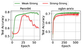
Weak-strong vs. strong-strong.     We implement a “strong-strong” variant of Mowst^$\star$ consisting of two GNN experts with identical network architecture. Figure 1 shows the convergence curves of the test set accuracy during training, with GCN as the strong experts’ architecture. On both Penn94 and ogbn-arxiv, we observe that the convergence quality of the “strong-strong” variant is much worse. Specifically, on Penn94, the “strong-strong” model eventually failed to identify a suitable collaboration mode between the two GNNs, causing the collapse of the accuracy curve. On ogbn-arxiv, the collapse of the “strong-strong” model does not happen. Yet it is still clear that 1. training a “weak-strong” model is more stable, indicated by the much smaller variance, and 2. the accuracy of the “strong-strong” variant is significantly lower. Lastly, note that the $x$-axis denotes number of epochs. The per-epoch execution time for “strong-strong” is also significantly longer, indicating an even longer overall convergence time than the “weak-strong” model.

Table 2: Comparison of test set accuracy.

	Flickr	pokec	twitch-gamer
Mowst-GCN (joint)	53.47$\pm$0.36	76.62$\pm$0.11	63.44$\pm$0.22
Mowst-GCN	54.62$\pm$0.23	77.12$\pm$0.09	63.74$\pm$0.23
Mowst$\star$-GCN	53.94$\pm$0.37	77.28$\pm$0.08	63.59$\pm$0.11

Mowst vs. Mowst^$\star$.     Using the GCN architecture as an example, we compare three model variants: 1. Mowst, 2. Mowst^$\star$ and 3. Mowst (joint), a vanilla version of Mowst that performs training by simultaneously updating the two experts from the gradients of the whole $L_{\text{{Mowst}}}$ (Equation 1). i.e., Mowst (joint) does not follow the “in-turn training” strategy discussed in Algorithm 2. From Table 2, we observe that 1. Mowst (joint) achieves lower test accuracy on all 3 graphs, 2. Mowst or Mowst^$\star$ may outperform the other variant depending on the property of the graph. Observation (1) shows the efficacy of our “in-turn training” strategy. Intuitively, since the two experts may have difference convergence rate, updating one expert with the other one fixed may help stabilize training and improve the overall convergence quality. Observation (2) is consistent with our tradeoff analysis in §2.5. Mowst^$\star$ can theoretically achieve a lower loss, while Mowst may be easier to optimize. In practice, both variants can be useful.

Training dynamics.     The two behaviors described in §2.4 may be observed on both Mowst and Mowst^$\star$. For demonstration, we visualize each behavior with one model variant.

Figure 2: Evolution of the $C$ distribution.

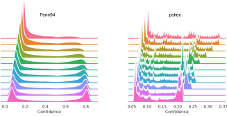
Specialization via data splitting.     We track the evolution of the confidence score $C$ during Mowst^$\star$-GCN training. In Figure 2, for each benchmark graph, we plot the distribution of $C$ generated by different snapshots of the model. The distribution on the upper side of the figure corresponds to earlier stage of training, while the distribution on the lower side reflects the relative weighting between the two experts when the training has converged well. In each distribution, the height shows the percentage of nodes assigned with such $C$. On Penn94, the GNN dominates initially. The MLP gradually learns to specialize on a significant portion of the data. Eventually, the whole graph is clearly split between the two experts, indicated by the two large peaks around 0 and 0.8 (corresponding to nodes assigned to GNN and MLP respectively). For pokec, the specialization is not so strong. When training progresses, the MLP becomes less confidence when the GNN is optimized better – nodes initially having larger $C$ gradually reduce $C$ to form a peak at around 0.2. For different graphs, the two experts will adapt their extent of collaboration by minimizing the confidence-weighted loss.

Figure 3: t-SNE visualization on GNN embeddings for Flickr.

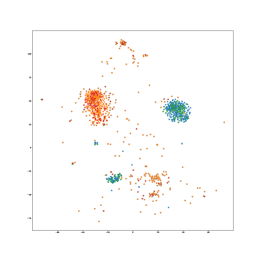
Denoised fine-tuning.     When this behavior emerges, the GNN expert has been optimized reasonably well and it dominates the MLP on almost all nodes. We focus on two distinct node groups and visualize their positions in a shared latent space by employing t-SNE (Van der Maaten & Hinton, 2008) on the second-to-last layer of the GNN expert, as illustrated in Figure 3. The first node group comprises those nodes that elicit high confidence from the MLP expert (nodes with top-25% $C$). The second group includes the remaining nodes. Green and blue dots represent the initial positions of the group 1 and 2 nodes at the end of training round $r$ (Algorithm 2). Red and orange dots represent the final positions of the group 1 and 2 nodes at the end of training round $r+10$. e.g., a node starting from a green dot will end at a red dot. Notably, we observe that a significant portion of nodes remains relatively stable throughout the training process, and thus their start and end positions almost completely overlap. We refrain from visualizing them, as their GNN’s predictions remain unaltered. Instead, we visualize only those nodes whose movement exceeds the 75^th percentile in terms of Euclidean distance. In Figure 3, the blue and green nodes are tightly clustered together, indicating that the GNN cannot differentiate them. After the MLP filters out the green nodes via high $C$, the GNN is then able to better optimize the blue nodes even if doing so will increase the GNN loss on the green ones (since the loss on green nodes is down-weighted). Eventually, the GNN pushes the blue nodes to a better position belonging to their true class (the shift of the green nodes is a side effect, as the GNN cannot differentiate the green from the blue ones). Overall, the blue nodes are originally misclassified but are corrected during this fine-tuning process enabled by the MLP expert’s denoising effect.

5 Conclusion

We presented a novel mixture-of-experts design to combine a weak MLP expert with a strong GNN expert for decoupling the self-feature and neighbor structure modalities in graphs. The “weak-strong” collaboration emerges under a gating mechanism based on the weak expert’s prediction confidence. We theoretically and empirically demonstrated intriguing training dynamics that evolve based on the properties of the graph and the relative strengths of the experts. We showed significant accuracy improvement over state-of-the-art on both homophilous and heterophilous graphs.

1Table of Contents (Appendix)   

Appendix A More Details on Experiments

A.1 Dataset statistics

Table 3 summarizes the basic statistics of the 6 benchmark graphs. Flickr is originally proposed in Zeng et al. (2020). ogbn-products and ogbn-arxiv are originally proposed in Hu et al. (2020). Penn94, pokec and twitch-gamer are originally proposed in Lim et al. (2021).

Table 3: Statistics of the datasets.

	# nodes	# edges	# classes	# node features
Flickr	89,250	899,756	7	500
ogbn-products	2,449,029	61,859,140	47	100
ogbn-arxiv	169,343	2,332,486	40	128
Penn94	41,554	1,362,229	2	5
pokec	1,632,803	30,622,564	2	65
twitch-gamer	168,114	6,797,557	2	7

A.2 Hyperparameters

We perform grid search within the entire hyperparameter space defined as follows. Note that for GPR-GNN (Chien et al., 2021) and AdaGCN (Sun et al., 2021), we use the same grid search as reported in their original papers.

• MLP, GCN, GraphSAGE, GAT, GIN: learning rate $lr\in\{.1,.01,.001\}$ for all graphs. For all the homophilous graphs, the dropout ratio is searched in $\{.1,.2,.3,.4,.5\}$, hidden dimension is set as 256 and the number of layers is 3 according to Hu et al. (2020). For the heterophilous graphs, we follow the same as Lim et al. (2021).

• GPR-GNN: $lr\in\{.01,.05,.002\}$, $\alpha\in\{.1,.2,.5,.9\}$, hidden dimension $\in\{16,32,64,128,256\}$.

• AdaGCN: $lr\in\{.01,.005,.001\}$, number of layers $\in\{5,10\}$, dropout ratio $\in\{.0,.5\}$.

• GraphMoE: $lr\in\{.1,.01,.001\}$, dropout ratio $\in\{.1,.2,.3,.4,.5\}$, number of experts $\in\{2,8\}$.

• Mowst and Mowst^$\star$: The learning rate and dropout ratio of the MLP expert and the GNN expert are kept the same. The girds for them are $lr\in\{.1,.01,.001\}$, dropout ratio $\in\{.1,.2,.3,.4,.5\}$. As for the gating module, we also conduct a grid search to find the optimal combination of the learning rate and dropout ratio. The grid for them are $lr\in\{.1,.01,.001\}$, dropout ratio $\in\{.1,.2,.3,.4,.5\}$.

A.3 Implementation details

We implement our code using PyTorch and the PyTorch Geometric library (for the GCN and GraphSAGE layers of Mowst(^$\star$)-GCN and Mowst(^$\star$)-SAGE). Training of our models and the baselines were conducted on NVIDIA A100 GPUs with 80GB memory. All trainings were conducted by full-batch gradient descent using Adam (Kingma & Ba, 2014) optimizer, without any neighborhood or subgraph sampling.

Appendix B Proof and Derivation

B.1 Proofs related to model optimization

Definition B.1.

(Convex function (Bertsekas et al., 2003)) Let $\mathcal{D}$ be a convex subset of $\mathbb{R}^{n}$. A function $f:\mathcal{D}\mapsto\mathbb{R}$ is convex if $f\left(\lambda\cdot x+\left(1-\lambda\right)\cdot y\right)\leq\lambda\cdot f\left(x\right)+\left(1-\lambda\right)\cdot f\left(y\right)$, $\forall x,y\in\mathcal{D}$ and $\forall\lambda\in[0,1]$.

Definition B.2.

(Quasiconvex function (Boyd & Vandenberghe, 2004)) Consider a real-valued function $f$ whose domain $\mathcal{D}$ is convex. Function $f$ is quasiconvex if for any $\gamma\in\mathbb{R}$, its $\gamma$-sublevel set $\{x\in\mathcal{D}\;|\;f(x)\leq\gamma\}$ is convex. Equivalently, $f$ is quasiconvex if, for all $x,y\in\mathcal{D}$ and $\lambda\in[0,1]$, we have $f\left(\lambda\cdot x+\left(1-\lambda\right)\cdot y\right)\leq\max\left\{f\left(x\right),f\left(y\right)\right\}$.

Definition B.3.

(Strictly quasiconvex function) A real-valued function $f$ defined on a convex domain $\mathcal{D}$ is strictly quasiconvex if, for all $x,y\in\mathcal{D}$, $x\neq y$ and $\lambda\in(0,1)$, we have $f\left(\lambda\cdot x+\left(1-\lambda\right)\cdot y\right)<\max\left\{f\left(x\right),f\left(y\right)\right\}$.

B.1.1 Proof of Proposition 2.2

Proposition B.4.

(Originally Proposition 2.2) $C=G\circ D$ is quasiconvex.

Proof.

The proof directly follows Agrawal & Boyd (2020), which states that if $g:\mathcal{D}\mapsto\mathbb{R}$ is a quasiconvex function and $h$ is a non-decreasing real-valued function on the real line, then $f=h\circ g$ is quasiconvex. By Definition 2.1, we have $C=G\circ D$ is quasiconvex.

Then the only thing remains to be shown is the quasiconvexity of typical dispersion functions. We show the convexity of the variance and negative entropy functions by following Definition B.1. Then we complete the proof since any convex function is also quasiconvex (based on Definitions B.1 and B.2: if $f$ is convex, then $f\left(\lambda x+\left(1-\lambda\right)y\right)\leq\lambda f(x)+\left(1-\lambda\right)f(y)\leq\lambda\max\{f(x),f(y)\}+\left(1-\lambda\right)\max\{f(x),f(y)\}=\max\{f(x),f(y)\}$).

To show convexity of the dispersion function $D\left(\bm{p}\right)$, we first note that its domain is a $\left(n-1\right)$-simplex (i.e., $\sum_{1\leq i\leq n}p_{i}=1$ and $p_{i}\geq 0$ for $i=1,2,\ldots,n$), which is a convex set. Next, for specific $D$:

Variance function

is defined as $D\left(\bm{p}\right)=\sum_{1\leq i\leq n}\left(p_{i}-\frac{1}{n}\right)^{2}$. For two points $\bm{p}$ and $\bm{p}^{\prime}$ and $\lambda\in[0,1]$, it is easy to show that $D\left(\lambda\bm{p}+\left(1-\lambda\right)\bm{p}^{\prime}\right)\leq\lambda D\left(\bm{p}\right)+\left(1-\lambda\right)D\left(\bm{p}^{\prime}\right)$ (we can follow a similar treatment as Equation B.1.3 by noting that scalar function $d(x)=\left(x-\frac{1}{n}\right)^{2}$ is convex).

Negative entropy function

is defined as $D\left(\bm{p}\right)=c+\sum_{1\leq i\leq n}p_{i}\cdot\log p_{i}$, where $c$ is just a constant to satisfy Definition 2.1 that $D\left(\frac{1}{n}\bm{1}\right)=0$. It is a well-known result that the negative entropy is convex. See for example the proof in JoramSoch (2020).

∎

B.1.2 Proof of Proposition 2.3

Proposition B.5.

(Originally Proposition 2.3) Given $\bm{\alpha}_{i}$, $\hat{L}_{\bm{\alpha}_{i}}\left(\hat{\bm{p}}_{i}\right)$ is a convex function of $\hat{\bm{p}}_{i}$ with unique minimizer $\hat{\bm{p}}_{i}^{*}=\bm{\alpha}_{i}$. Let $\Delta\left(\bm{\alpha}\right)=\hat{L}_{\bm{\alpha}}\left(\bm{\alpha}\right)$ be a function of $\bm{\alpha}$, $\Delta$ is a concave function with unique maximizer $\bm{\alpha}^{*}=\frac{1}{n}\bm{1}$.

Proof.

We can formulate the problem of finding the minimizer $\hat{\bm{p}}_{i}^{*}$ of $\hat{L}_{\bm{\alpha}_{i}}\left(\hat{\bm{p}}_{i}\right)$ as

$$\min_{\hat{\bm{p}}_{i}}\quad -\sum_{1\leq j\leq n}\alpha_{ij}\cdot\log\hat{p}_{ij}$$ (4)

s.t. $$\hat{p}_{ij}\geq 0,\textrm{ for }j=1,2,...n$$ (5)

$$\sum_{1\leq j\leq n}\hat{p}_{ij}=1$$ (6)

The Larangian is

$$\mathcal{L}\left(\hat{\bm{p}}_{i},\gamma,\lambda_{1},\lambda_{2},...,\lambda_{n}\right)=\sum_{1\leq j\leq n}\alpha_{ij}\cdot\log\hat{p}_{ij}+\gamma\left(\sum_{1\leq j\leq n}\hat{p}_{ij}-1\right)+\sum_{1\leq j\leq n}{\lambda_{j}\hat{p}_{ij}}$$ (7)

Applying the KKT condition (Bertsekas, 2009), we have

$$\begin{cases}\begin{aligned} &\alpha_{ij}\cdot\frac{1}{\hat{p}^{*}_{ij}}+\gamma^{*}+\lambda^{*}_{j}=0,&\textrm{for }j=1,2,...,n\quad&\textrm{ (Stationarity)}\\ &\lambda_{j}^{*}\cdot\hat{p}^{*}_{ij}=0,&\textrm{ for }j=1,2,...,n\quad&\textrm{ (Complementary slackness)}\\ &\hat{p}^{*}_{ij}\geq 0,&\textrm{ for }j=1,2,...,n\quad&\textrm{ (Primal feasibility)}\\ &\sum_{1\leq j\leq n}{\hat{p}^{*}_{ij}}=1&\quad&\textrm{ (Primal feasibility)}\\ &\lambda^{*}_{j}\geq 0&\textrm{ for }j=1,2,...,n\quad&\textrm{ (Dual feasibility)}\\ &\gamma^{*}\geq 0&\quad&\textrm{ (Dual feasibility)}\end{aligned}\end{cases}$$ (8)

Solving the system of equations in 8, we have $\hat{p}^{*}_{ij}=\alpha_{ij}/\left(\sum_{1\leq j\leq n}{\alpha_{ij}}\right)$. Since $\bm{\alpha}_{i}$ forms a distribution, we further have $\hat{p}^{*}_{ij}=\alpha_{ij}$, i.e.,

$$\hat{\bm{p}}_{i}^{*}=\bm{\alpha}_{i}$$ (9)

Since $\hat{L}_{\bm{\alpha_{i}}}$ is also strictly convex (Proposition B.7), its minimizer is unique.

In particular, $\Delta\left(\bm{\alpha}_{i}\right)=\hat{L}_{\bm{\alpha}_{i}}\left(\bm{\alpha}_{i}\right)=-\sum_{1\leq j\leq n}\alpha_{ij}\cdot\log\alpha_{ij}=\mathcal{H}\left(\bm{\alpha}_{i}\right)$. It is easy to show that the entropy function $\mathcal{H}$ is strictly concave w.r.t. the probability mass function and attains its maximum when $\bm{\alpha}_{i}^{*}=\frac{1}{n}\bm{1}$ (JoramSoch, 2020).

∎

B.1.3 Proof of Theorem 2.4 and Corollary 2.4.1

We first observe that the optimization problem defined in Equation 2 can be fully decomposed:

$$\min_{\{\hat{\bm{p}}_{i}\}}\sum_{1\leq i\leq m}C\left(\hat{\bm{p}}_{i}\right)\cdot\left(\hat{L}_{\bm{\alpha}_{i}}\left(\hat{\bm{p}}_{i}\right)-\mu_{i}\right)=\sum_{1\leq i\leq m}\min_{\hat{\bm{p}}_{i}}\left(C\left(\hat{\bm{p}}_{i}\right)\cdot\left(\hat{L}_{\bm{\alpha}_{i}}\left(\hat{\bm{p}}_{i}\right)-\mu_{i}\right)\right)$$ (10)

It clearly follows that we can break down the original optimization problem 2 into $m$ independent sub-problems:

$$\hat{\bm{p}}_{i}^{*}=\arg\min_{\hat{\bm{p}}_{i}}\left(C\left(\hat{\bm{p}}_{i}\right)\cdot\left(\hat{L}_{\bm{\alpha}_{i}}\left(\hat{\bm{p}}_{i}\right)-\mu_{i}\right)\right),\qquad 1\leq i\leq m$$ (11)

Therefore, in the following, we omit the subscript $i$.

Definition B.6.

(Extreme points (Bertsekas et al., 2003)) Given a nonempty convex set $\mathcal{D}$, a point $x\in\mathcal{D}$ is an extreme point if there do not exist $y\in\mathcal{D}$ and $z\in\mathcal{D}$ with $y\neq x$ and $z\neq x$, and a scalar $\lambda\in(0,1)$, such that $x=\lambda y+\left(1-\lambda\right)z$.

Proposition B.7.

The loss function $\hat{L}_{\bm{\alpha}}\left(\hat{\bm{p}}\right)$ is strictly convex. For all $\mu$, the sub-level set $\mathcal{L}_{\bm{\alpha}}^{\leq\mu}$ is convex and compact.

Proof.

For strict convexity, first of all, the domain of $\hat{L}_{\bm{\alpha}}$, the $\left(n-1\right)$-simplex, is convex. Then consider two points $\hat{\bm{p}}$ and $\hat{\bm{p}}^{\prime}$ in $\hat{L}_{\bm{\alpha}}$’s domain and some $\lambda\in(0,1)$:

$$\hat{L}_{\bm{\alpha}}\left(\lambda\cdot\hat{\bm{p}}+\left(1-\lambda\right)\cdot\hat{\bm{p}}^{\prime}\right)= -\sum_{1\leq i\leq n}\alpha_{i}\cdot\log\left(\lambda\cdot\hat{p}_{i}+\left(1-\lambda\right)\cdot\hat{p}_{i}^{\prime}\right)$$

$$\stackrel{{\scriptstyle(a)}}{{<}} \sum_{1\leq i\leq n}\alpha_{i}\cdot\left(-\lambda\cdot\log\hat{p}_{i}-\left(1-\lambda\right)\cdot\log\hat{p}_{i}^{\prime}\right)$$

$$= \lambda\cdot\left(-\sum_{1\leq i\leq n}\alpha_{i}\cdot\log\hat{p}_{i}\right)+\left(1-\lambda\right)\cdot\left(-\sum_{1\leq i\leq n}\alpha_{i}\cdot\log\hat{p}_{i}^{\prime}\right)$$

$$= \lambda\cdot\hat{L}_{\bm{\alpha}}\left(\hat{\bm{p}}\right)+\left(1-\lambda\right)\cdot\hat{L}_{\bm{\alpha}}\left(\hat{\bm{p}}^{\prime}\right)$$ (12)

where “(a)” is due to the strict convexity of the $\log$ function. This proves that $\hat{L}_{\bm{\alpha}}$ is strictly convex. Then it directly follows that all its sub-level sets are convex.

Note that $\hat{L}_{\bm{\alpha}}$ is continuous (and so lower semicontinuous as well). By Proposition 1.2.2 of Bertsekas et al. (2003), all sublevel sets of $\hat{L}_{\bm{\alpha}}$ are closed. Further, since $\hat{L}_{\bm{\alpha}}$ is defined on the $\left(n-1\right)$-simplex, $\mathcal{L}_{\bm{\alpha}}^{\leq\mu}$ is also bounded. So $\mathcal{L}_{\bm{\alpha}}^{\leq\mu}$ is compact (compact means closed and bounded). ∎

Proposition B.8.

The set of extreme points of $\mathcal{L}_{\bm{\alpha}}^{\leq\mu}$ equals $\mathcal{L}_{\bm{\alpha}}^{\mu}$.

Proof.

Denote $\mathcal{P}$ as the set of extreme points of $\mathcal{L}_{\bm{\alpha}}^{\leq\mu}$. We first show that $\mathcal{L}_{\bm{\alpha}}^{\mu}\subseteq\mathcal{P}$. Consider a point $\hat{\bm{p}}_{0}\in\mathcal{L}_{\bm{\alpha}}^{\mu}$. Suppose there exist some other points $\hat{\bm{p}}_{1},\hat{\bm{p}}_{2}\in\mathcal{L}_{\bm{\alpha}}^{\leq\mu}$ (with $\hat{\bm{p}}_{1}\neq\hat{\bm{p}}_{0}$ and $\hat{\bm{p}}_{2}\neq\hat{\bm{p}}_{0}$), such that $\lambda\hat{\bm{p}}_{1}+\left(1-\lambda\right)\hat{\bm{p}}_{2}=\hat{\bm{p}}_{0}$ for some $\lambda\in(0,1)$. By strict convexity shown in Proposition B.7, we have $\mu=\hat{L}_{\bm{\alpha}}\left(\hat{\bm{p}}_{0}\right)=\hat{L}_{\bm{\alpha}}\left(\lambda\hat{\bm{p}}_{1}+\left(1-\lambda\right)\hat{\bm{p}}_{2}\right)<\lambda\hat{L}_{\bm{\alpha}}\left(\hat{\bm{p}}_{1}\right)+\left(1-\lambda\right)\hat{L}_{\bm{\alpha}}\left(\hat{\bm{p}}_{2}\right)$. This implies that $\hat{L}_{\bm{\alpha}}\left(\hat{\bm{p}}_{1}\right)>\mu$ or $\hat{L}_{\bm{\alpha}}\left(\hat{\bm{p}}_{2}\right)>\mu$, which contradicts with the condition that $\hat{\bm{p}}_{1},\hat{\bm{p}}_{2}\in\mathcal{L}_{\bm{\alpha}}^{\leq\mu}$. Thus, any point $\hat{\bm{p}}_{0}\in\mathcal{L}_{\bm{\alpha}}^{\mu}$ is an extreme point of $\mathcal{L}_{\bm{\alpha}}^{\leq\mu}$.

Now we show $\mathcal{P}\subseteq\mathcal{L}_{\bm{\alpha}}^{\mu}$. Consider a point $\hat{\bm{p}}_{0}\in\mathcal{L}_{\bm{\alpha}}^{<\mu}$. For any $\mu\in\mathbb{R}$, we always have $\hat{p}_{0i}>0$, for all $i=1,2,\ldots,n$ (otherwise, $\hat{L}_{\bm{\alpha}}\left(\hat{\bm{p}}_{0}\right)\rightarrow\infty$). This means that we can find a vector $\bm{\epsilon}$, such that 1. $\sum_{1\leq i\leq n}\epsilon_{i}=0$, 2. $|\epsilon_{i}|<\hat{p}_{0i}$, for all $1\leq i\leq n$, and 3. $\hat{L}_{\bm{\alpha}}\left(\hat{\bm{p}}_{0}+\bm{\epsilon}\right)\leq\mu$and $\hat{L}_{\bm{\alpha}}\left(\hat{\bm{p}}_{0}-\bm{\epsilon}\right)\leq\mu$. Point (1) and (2) ensure that $\hat{\bm{p}}_{0}+\bm{\epsilon}$ and $\hat{\bm{p}}_{0}-\bm{\epsilon}$ are both with the domain of $\hat{L}_{\bm{{\alpha}}}$. For Point (3), we can always find small enough $\epsilon_{i}$ due to the continuity of the loss function $\hat{L}_{\bm{\alpha}}$. We thus find two points, $\hat{\bm{p}}_{1}=\hat{\bm{p}}_{0}+\bm{\epsilon}\in\mathcal{L}_{\bm{\alpha}}^{\leq\mu}$ and $\hat{\bm{p}}_{2}=\hat{\bm{p}}_{0}-\bm{\epsilon}\in\mathcal{L}_{\bm{\alpha}}^{\leq\mu}$, where $\hat{\bm{p}}_{0}=\frac{1}{2}\hat{\bm{p}}_{1}+\frac{1}{2}\hat{\bm{p}}_{2}$. Thus, $\hat{\bm{p}}_{0}\in\mathcal{L}_{\bm{\alpha}}^{<\mu}$ is not an extreme point of $\mathcal{L}_{\bm{\alpha}}^{\leq\mu}$.

In summary, $\mathcal{P}=\mathcal{L}_{\bm{\alpha}}^{\mu}$. ∎

Proposition B.9.

(Krein-Milman Theorem (Bertsekas et al., 2003)) Let $\mathcal{D}$ be a nonempty convex subset of $\mathbb{R}^{n}$. If $\mathcal{D}$ is compact, then $\mathcal{D}$ is equal to the convex hull of its extreme points.

Proposition B.10.

(Caratheodory’s Theorem (Bertsekas, 2009)) Let $\mathcal{D}$ be a nonempty subset of $\mathbb{R}^{n}$. Every point from the convex hull of $\mathcal{D}$ can be represented as a convex combination of $x_{1},\ldots,x_{m}$ from $\mathcal{D}$, where $m\leq n+1$ and $x_{2}-x_{1},\ldots,x_{m}-x_{1}$ are linearly independent.

Proposition B.11.

If $f$ is a quasiconvex function defined on $\mathcal{D}$, then for all $x_{1},\ldots,x_{m}\in\mathcal{D}$ and $\lambda_{1}\geq 0,\ldots,\lambda_{m}\geq 0$ such that $\sum_{1\leq i\leq m}\lambda_{i}=1$, we have $f\left(\sum_{1\leq i\leq m}\lambda_{i}x_{i}\right)\leq\max_{1\leq i\leq m}\{f\left(x_{i}\right)\}$.

Proposition B.12.

If $f$ is a strictly quasiconvex function defined on $\mathcal{D}$, then for 1. $x_{1},\ldots,x_{m}\in\mathcal{D}$such that $x_{1}\neq x_{2}\ldots\neq x_{m}$ and $x_{2}-x_{1},\ldots,x_{m}-x_{1}$ are linearly independent, and 2. $\lambda_{1}>0,\ldots,\lambda_{m}>0$such that $\sum_{1\leq i\leq m}\lambda_{i}=1$, we have $f\left(\sum_{1\leq i\leq m}\lambda_{i}x_{i}\right)<\max_{1\leq i\leq m}\{f\left(x_{i}\right)\}$.

Proof.

For brevity, we only show the proof for Proposition B.12 as the proof for Proposition B.11 is similar (and easier). We prove by induction. The base case of $m=2$ automatically holds by Definition B.2.

For $m>2$, note that

$$\sum_{1\leq i\leq m}\lambda_{i}x_{i}=\lambda_{1}x_{1}+\left(\sum_{2\leq i\leq m}\lambda_{i}\right)\cdot\left(\sum_{2\leq j\leq m}\frac{\lambda_{j}}{\sum_{2\leq i\leq m}\lambda_{i}}x_{j}\right)$$ (13)

Let $\lambda_{j}^{\prime}=\frac{\lambda_{j}}{\sum_{2\leq i\leq m}\lambda_{i}}$. Apparently, $\sum_{2\leq j\leq m}\lambda_{j}^{\prime}=1$ and $\lambda_{j}^{\prime}>0$ for all $2\leq j\leq m$. In addition, $x_{3}-x_{2},\ldots,x_{m}-x_{2}$ are linearly independent (To show this: $\sum_{2\leq j\leq m}\beta_{j}\left(x_{j}-x_{1}\right)=\sum_{3\leq j\leq m}\beta_{j}\left(x_{j}-x_{2}\right)+\left(\sum_{2\leq j\leq m}\beta_{j}\right)\left(x_{2}-x_{1}\right)$. If $x_{3}-x_{2},\ldots,x_{m}-x_{2}$ are linearly dependent, then there exists $\beta_{3},\ldots,\beta_{m}$ such that $\sum_{3\leq j\leq m}\beta_{j}\left(x_{j}-x_{2}\right)=0$. Then by letting $\beta_{2}=-\sum_{3\leq j\leq m}\beta_{j}$, we have $\sum_{2\leq j\leq m}\beta_{j}\left(x_{j}-x_{1}\right)=0$ – contradiction with the hypothesis that $x_{2}-x_{1},\ldots,x_{m}-x_{1}$ are linearly independent). Therefore, by induction hypothesis, we have

$$f\left(\sum_{2\leq j\leq m}\lambda_{j}^{\prime}x_{j}\right)<\max_{2\leq j\leq m}\{f\left(x_{j}\right)\}$$ (14)

Let $x^{\prime}=\sum_{2\leq j\leq m}\lambda_{j}^{\prime}x_{j}$. Since $x_{2}-x_{1},\ldots,x_{m}-x_{1}$ are linearly independent, we must have $\sum_{2\leq j\leq m}\lambda_{j}^{\prime}\left(x_{j}-x_{1}\right)\neq 0$. Equivalently, $\sum_{2\leq j\leq m}\lambda_{j}^{\prime}x_{j}=x^{\prime}\neq x_{1}$. Thus,

$$f\left(\sum_{1\leq i\leq m}\lambda_{i}x_{i}\right)= f\left(\lambda_{1}x_{1}+\left(1-\lambda_{1}\right)x^{\prime}\right)<\max\{f\left(x_{1}\right),f\left(x^{\prime}\right)\}$$ (15)

$$< \max\left\{f\left(x_{1}\right),\max_{2\leq i\leq m}\{f\left(x_{i}\right)\}\right\}$$ (16)

$$= \max_{1\leq i\leq m}\{f\left(x_{i}\right)\}$$ (17)

This completes the induction process and thus concludes the proof. ∎

Theorem B.13.

(Originally Theorem 2.4) Suppose $C=G\circ D$ follows Definition 2.1. Denote $\mathcal{L}_{\bm{\alpha}}^{\mu}=\{\hat{\bm{p}}\;|\;\hat{L}_{\bm{\alpha}}\left(\hat{\bm{p}}\right)=\mu\}$ and $\mathcal{L}_{\bm{\alpha}}^{<\mu}=\{\hat{\bm{p}}\;|\;\hat{L}_{\bm{\alpha}}\left(\hat{\bm{p}}\right)<\mu\}$ as the level set and strict sublevel set of $\hat{L}_{\bm{\alpha}}$. Denote $\mathcal{C}^{<\mu}=\{\hat{\bm{p}}\;|\;C\left(\hat{\bm{p}}\right)<\mu\}$ as the strict sublevel set of $C$. For a given $\bm{\alpha}\neq\frac{1}{n}\bm{1}_{n}$, the minimizer $\hat{\bm{p}}^{*}$ satisfies:

• If $\Delta\left(\bm{\alpha}\right)>\mu$, then $\hat{\bm{p}}^{*}=\frac{1}{n}\bm{1}_{n}$ and $C\left(\hat{\bm{p}}^{*}\right)=0$.

• If $\Delta\left(\bm{\alpha}\right)=\mu$, then $\hat{\bm{p}}^{*}=\bm{\alpha}$ or $\hat{\bm{p}}^{*}=\frac{1}{n}\bm{1}$.

• If $\Delta\left(\bm{\alpha}\right)<\mu$, then $\hat{\bm{p}}^{*}\in\mathcal{L}_{\bm{\alpha}}^{<\mu}-\mathcal{C}^{<\mu^{\prime}}$ where $\mu^{\prime}=C\left(\bm{\alpha}\right)\leq C\left(\hat{\bm{p}}^{*}\right)\leq G\left(\max_{\hat{\bm{p}}\in\mathcal{L}_{\bm{\alpha}}^{\mu}}D\left(\hat{\bm{p}}\right)\right)$. Further, there exists $C$ such that $\hat{\bm{p}}^{*}=\bm{\alpha}$, or $\hat{\bm{p}}^{*}$ is sufficiently close to the level set $\mathcal{L}_{\bm{\alpha}}^{\mu}$.

Proof.

We separately consider the three cases listed by Theorem 2.4.

Case 1.

By Proposition 2.3, we have $\hat{L}_{\bm{\alpha}}\left(\hat{\bm{p}}\right)-\mu\geq\min_{\hat{\bm{p}}}\left(\hat{L}_{\bm{\alpha}}\left(\hat{\bm{p}}\right)-\mu\right)=\hat{L}_{\bm{\alpha}}\left(\bm{\alpha}\right)-\mu=\Delta\left(\bm{\alpha}\right)-\mu>0$ for all $\hat{\bm{p}}$. By Definition 2.1, we have $C\left(\hat{\bm{p}}\right)\geq 0$ for all $\hat{\bm{p}}$. We can thus derive the following bound: $C\left(\hat{\bm{p}}^{*}\right)\cdot\left(\hat{L}_{\bm{\alpha}}\left(\hat{\bm{p}}^{*}\right)-\mu\right)=\min_{\hat{\bm{p}}}\left(C\left(\hat{\bm{p}}\right)\cdot\left(\hat{L}_{\bm{\alpha}}\left(\hat{\bm{p}}\right)-\mu\right)\right)\geq 0$. Further, since $\hat{L}_{\bm{\alpha}}\left(\hat{\bm{p}}\right)-\mu>0$ for all $\hat{\bm{p}}$, the lower bound $C\left(\hat{\bm{p}}^{*}\right)\cdot\left(\hat{L}_{\bm{\alpha}}\left(\hat{\bm{p}}^{*}\right)-\mu\right)=0$ is achieved if and only if $C\left(\hat{\bm{p}}^{*}\right)=0$. By Definition 2.1, the minimizer $\hat{\bm{p}}^{*}=\frac{1}{n}\bm{1}_{n}$.

Case 2.

The reasoning is similar to Case 1. We can derive $C\left(\hat{\bm{p}}^{*}\right)\cdot\left(\hat{L}_{\bm{\alpha}}\left(\hat{\bm{p}}^{*}\right)-\mu\right)\geq 0$. Now to achieve the lower bound $C\left(\hat{\bm{p}}^{*}\right)\cdot\left(\hat{L}_{\bm{\alpha}}\left(\hat{\bm{p}}^{*}\right)-\mu\right)=0$, we either need $C\left(\hat{\bm{p}}^{*}\right)=0$ or $\hat{L}_{\bm{\alpha}}\left(\hat{\bm{p}}^{*}\right)-\mu=0$, which means either $\hat{\bm{p}}^{*}=\frac{1}{n}\bm{1}_{n}$ or $\hat{\bm{p}}^{*}=\bm{\alpha}$.

Case 3.

First, observe that $C\left(\hat{\bm{p}}^{*}\right)\cdot\left(\hat{L}_{\bm{\alpha}}\left(\hat{\bm{p}}^{*}\right)-\mu\right)=\min_{\hat{\bm{p}}}\left(C\left(\hat{\bm{p}}\right)\cdot\left(\hat{L}_{\bm{\alpha}}\left(\hat{\bm{p}}\right)-\mu\right)\right)\stackrel{{\scriptstyle\hat{\bm{p}}=\bm{\alpha}}}{{\leq}}C\left(\bm{\alpha}\right)\cdot\left(\hat{L}_{\bm{\alpha}}\left(\bm{\alpha}\right)-\mu\right)=C\left(\bm{\alpha}\right)\cdot\left(\Delta\left(\bm{\alpha}\right)-\mu\right)<0$ (note that we assume $\bm{\alpha}\neq\frac{1}{n}\bm{1}_{n}$). Since $C\left(\hat{\bm{p}}\right)\geq 0$ for all $\hat{\bm{p}}$, this implies that

$$C\left(\hat{\bm{p}}^{*}\right)>0$$ (18)

$$\hat{L}_{\bm{\alpha}}\left(\hat{\bm{p}}^{*}\right)-\mu<0$$ (19)

By inequality 19, we have $\hat{\bm{p}}^{*}\in\mathcal{L}_{\bm{\alpha}}^{<\mu}$.

We can further constrain $\hat{\bm{p}}^{*}$ such that $C\left(\hat{\bm{p}}^{*}\right)\geq C\left(\bm{\alpha}\right)$: Suppose otherwise that $0\leq C\left(\hat{\bm{p}}^{*}\right)<C\left(\bm{\alpha}\right)$. By Proposition 2.3, we have $\hat{L}_{\bm{\alpha}}\left(\hat{\bm{p}}^{*}\right)-\mu\geq\Delta\left(\bm{\alpha}\right)-\mu\quad\Rightarrow\quad-\left(\hat{L}_{\bm{\alpha}}\left(\hat{\bm{p}}^{*}\right)-\mu\right)\leq-\left(\Delta\left(\bm{\alpha}\right)-\mu\right)$. Combining the two inequalities together, we have $-C\left(\hat{\bm{p}}^{*}\right)\cdot\left(\hat{L}_{\bm{\alpha}}\left(\hat{\bm{p}}^{*}\right)-\mu\right)<-C\left(\bm{\alpha}\right)\cdot\left(\Delta\left(\bm{\alpha}\right)-\mu\right)\quad\Rightarrow\quad C\left(\hat{\bm{p}}^{*}\right)\cdot\left(\hat{L}_{\bm{\alpha}}\left(\hat{\bm{p}}^{*}\right)-\mu\right)>C\left(\bm{\alpha}\right)\cdot\left(\Delta\left(\bm{\alpha}\right)-\mu\right)$. This means that $\hat{\bm{p}}^{*}$ is not a minimizer – a contradiction. In other words, we must have $\hat{\bm{p}}^{*}\not\in\mathcal{C}^{<\mu^{\prime}}$ where $\mu^{\prime}=C\left(\bm{\alpha}\right)$.

So far, we have proven $\hat{\bm{p}}^{*}\in\mathcal{L}_{\bm{\alpha}}^{<\mu}-\mathcal{C}^{<\mu^{\prime}}$ where $\mu^{\prime}=C\left(\bm{\alpha}\right)\leq C\left(\hat{\bm{p}}^{*}\right)$. Next, we further upper-bound the range of the confidence corresponding to $\hat{\bm{p}}^{*}$. Note that

$$C\left(\hat{\bm{p}}^{*}\right)\leq\sup_{\hat{\bm{p}}\in\mathcal{L}_{\bm{\alpha}}^{<\mu}-\mathcal{C}^{<\mu^{\prime}}}C\left(\hat{\bm{p}}\right)\stackrel{{\scriptstyle(a)}}{{\leq}}\sup_{\hat{\bm{p}}\in\mathcal{L}_{\bm{\alpha}}^{\leq\mu}}C\left(\hat{\bm{p}}\right)\stackrel{{\scriptstyle(b)}}{{=}}G\left(\max_{\hat{\bm{p}}\in\mathcal{L}_{\bm{\alpha}}^{\leq\mu}}D\left(\hat{\bm{p}}\right)\right)\stackrel{{\scriptstyle(c)}}{{=}}G\left(\max_{\hat{\bm{p}}\in\mathcal{L}_{\bm{\alpha}}^{\mu}}D\left(\hat{\bm{p}}\right)\right)$$ (20)

For “$\stackrel{{\scriptstyle(a)}}{{\leq}}$” above, the reason is that $\mathcal{L}_{\bm{\alpha}}^{<\mu}-\mathcal{C}^{<\mu^{\prime}}\subseteq\mathcal{L}_{\bm{\alpha}}^{\leq\mu}$. For “$\stackrel{{\scriptstyle(b)}}{{=}}$”, let’s first consider $\sup_{\mathcal{L}_{\bm{\alpha}}^{\leq\mu}}D\left(\hat{\bm{p}}\right)$. By Proposition B.7, $\mathcal{L}_{\bm{\alpha}}^{\leq\mu}$ is compact. By Definition 2.1, $D$ is continuous. So by the extreme value theorem (Murphy, 2008), $D$ attains its maximum value. i.e., there exists $\hat{\bm{p}}^{\prime}\in\mathcal{L}_{\bm{\alpha}}^{\leq\mu}$ such that $D\left(\hat{\bm{p}}^{\prime}\right)=\sup_{\mathcal{L}_{\bm{\alpha}}^{\leq\mu}}D\left(\hat{\bm{p}}\right)=\max_{\mathcal{L}_{\bm{\alpha}}^{\leq\mu}}D\left(\hat{\bm{p}}\right)$. In other words, $D\left(\hat{\bm{p}}^{\prime}\right)\geq D\left(\hat{\bm{p}}\right)$ for all $\hat{\bm{p}}\in\mathcal{L}_{\bm{\alpha}}^{\leq\mu}$. Now since $G$ is monotonically non-decreasing (Definition 2.1), we have $G\left(D\left(\hat{\bm{p}}^{\prime}\right)\right)\geq G\left(D\left(\hat{\bm{p}}\right)\right)$ for all $\hat{\bm{p}}\in\mathcal{L}_{\bm{\alpha}}^{\leq\mu}$. This means $C=G\circ D$ attains its maximum at $\hat{\bm{p}}^{\prime}$ and $\sup_{\hat{\bm{p}}\in\mathcal{L}_{\bm{\alpha}}^{\leq\mu}}C\left(\hat{\bm{p}}\right)=\max_{\hat{\bm{p}}\in\mathcal{L}_{\bm{\alpha}}^{\leq\mu}}C\left(\hat{\bm{p}}\right)=G\left(\max_{\hat{\bm{p}}\in\mathcal{L}_{\bm{\alpha}}^{\leq\mu}}D\left(\hat{\bm{p}}\right)\right)$. Finally, for “$\stackrel{{\scriptstyle(c)}}{{=}}$”, we need to show $\max_{\hat{\bm{p}}\in\mathcal{L}_{\bm{\alpha}}^{\leq\mu}}D\left(\hat{\bm{p}}\right)=\max_{\hat{\bm{p}}\in\mathcal{L}_{\bm{\alpha}}^{\mu}}D\left(\hat{\bm{p}}\right)$. By Proposition B.7, B.8 and B.9, $\mathcal{L}_{\bm{\alpha}}^{\leq\mu}$ is the convex hull of $\mathcal{L}_{\bm{\alpha}}^{\mu}$. So by Proposition B.10, for any point $\hat{\bm{p}}_{0}\in\mathcal{L}_{\bm{\alpha}}^{\leq\mu}$, we can find $\hat{\bm{p}}_{1},\ldots,\hat{\bm{p}}_{m}\in\mathcal{L}_{\bm{\alpha}}^{\mu}$ (with $m\leq n+1$), such that $\hat{\bm{p}}_{0}=\sum_{1\leq i\leq m}\lambda_{i}\hat{\bm{p}}_{i}$ (with $\sum_{1\leq i\leq m}\lambda_{i}=1$ and $\lambda_{i}\geq 0$ for $i=1,\ldots,m$). By Proposition B.11, we have $D\left(\hat{\bm{p}}_{0}\right)\leq\max_{1\leq i\leq m}\{D\left(\hat{\bm{p}}_{i}\right)\}\leq\max_{\hat{\bm{p}}\in\mathcal{L}_{\bm{\alpha}}^{\mu}}D\left(\hat{\bm{p}}\right)$. Thus, $\max_{\hat{\bm{p}}\in\mathcal{L}_{\bm{\alpha}}^{\leq\mu}}D\left(\hat{\bm{p}}\right)=\max_{\hat{\bm{p}}\in\mathcal{L}_{\bm{\alpha}}^{\mu}}D\left(\hat{\bm{p}}\right)$. This completes the proof for Equation 20. Thus, we have proven the bound on both the minimizer $\hat{\bm{p}}^{*}$ and its corresponding $C\left(\hat{\bm{p}}^{*}\right)$.

Case 3: tightness of the bound.

From the above proof, we know that when $\Delta\left(\bm{\alpha}\right)<\mu$, the possible positions that the minimizer $\hat{\bm{p}}^{*}$ can take are determined by the two level sets $\mathcal{C}^{<\mu^{\prime}}$ ($\mu^{\prime}=C\left(\bm{\alpha}\right)$) and $\mathcal{L}_{\bm{\alpha}}^{<\mu}$. We now show that the bound on $\hat{\bm{p}}^{*}$ is tight since $\hat{\bm{p}}^{*}$ can be close to the two level sets under appropriate $C=G\circ D$ function. Note that all our proof is based on $C$ defined by 2.1, meaning that $C$ does not need to be continuous.

First, we construct a $C$ such that $\hat{\bm{p}}^{*}=\bm{\alpha}$. Such a $C$ can be defined by a simple $G$ for any $D$:

$$G(x)=\begin{cases}0,\qquad&\text{when }x\leq 0\\ 1,&\text{when }x>0\end{cases}$$ (21)

Since $\bm{\alpha}\neq\frac{1}{n}\bm{1}_{n}$, we have $D\left(\bm{\alpha}\right)>0$ and thus $C\left(\bm{\alpha}\right)=G\left(D\left(\bm{\alpha}\right)\right)=1$. By conditions 18, 19, we have $C\left(\hat{\bm{p}}^{*}\right)\cdot\left(\hat{L}_{\bm{\alpha}}\left(\hat{\bm{p}}^{*}\right)-\mu\right)\geq\max C\left(\hat{\bm{p}}\right)\cdot\min\left(\hat{L}_{\bm{\alpha}}\left(\hat{\bm{p}}\right)-\mu\right)=1\cdot\left(\Delta\left(\bm{\alpha}\right)-\mu\right)=\Delta\left(\bm{\alpha}\right)-\mu$. In addition, since the problem $\min\left(\hat{L}_{\bm{\alpha}}\left(\hat{\bm{p}}\right)-\mu\right)$ has a unique minimizer at $\bm{\alpha}$ (Proposition 2.3), and $C\left(\bm{\alpha}\right)=\max C\left(\hat{\bm{p}}\right)=1$, we know that under $C$ defined by Equation 21, we have a unique minimizer $\hat{\bm{p}}^{*}=\bm{\alpha}$ for the overall optimization problem 11.

Next, we construct a $C$ such that $\hat{\bm{p}}^{*}$ is close to $\hat{L}_{\bm{\alpha}}^{\mu}$. We first define the distance between a point $\hat{\bm{p}}$ and the level set $\mathcal{L}_{\bm{\alpha}}^{\mu}$ as:

$${\text{dist}\left(\hat{\bm{p}},\mathcal{L}_{\bm{\alpha}}^{\mu}\right)}=\min_{\hat{\bm{p}}^{\prime}\in\mathcal{L}_{\bm{\alpha}}^{\mu}}\|\hat{\bm{p}}-\hat{\bm{p}}^{\prime}\|$$ (22)

Thus, we want to show that there exists a $C$, such that ${\text{dist}\left(\hat{\bm{p}}^{*},\mathcal{L}_{\bm{\alpha}}^{\mu}\right)}<\epsilon$ for any $\epsilon>0$.

Consider another sub-level set $\mathcal{L}_{\bm{\alpha}}^{\leq\mu-\eta}$ for some $\eta>0$ (we also let $\eta$ to be small enough so that $\mathcal{L}_{\bm{\alpha}}^{\leq\mu-\eta}$ is non-empty). We have shown before (by combining Propositions B.7, B.8, B.9 and B.10) that any point $\hat{\bm{p}}^{\prime}\in\mathcal{L}_{\bm{\alpha}}^{<\mu-\eta}$ can be expressed as a convex combination of $\hat{\bm{p}}_{1},\ldots,\hat{\bm{p}}_{m}$, where $m\leq n+1$, $\hat{\bm{p}}_{i}\in\mathcal{L}_{\bm{\alpha}}^{\mu-\eta}$ and $\hat{\bm{p}}_{2}-\hat{\bm{p}}_{1},\ldots,\hat{\bm{p}}_{m}-\hat{\bm{p}}_{1}$ are linearly independent. Since $\hat{\bm{p}}^{\prime}$ is in the strict sub-level set and $\hat{\bm{p}}_{i}$ are in the sub-level set, we have $\hat{\bm{p}}^{\prime}\neq\hat{\bm{p}}_{i}$, and thus we can write $\hat{\bm{p}}^{\prime}=\sum_{1\leq i\leq m}\lambda_{i}\hat{\bm{p}}_{i}$ where $\lambda_{i}>0$ and $\sum_{1\leq i\leq m}\lambda_{i}=1$.

Suppose $D$ is strictly quasiconvex. We can now apply Proposition B.12, such that

$$D\left(\hat{\bm{p}}^{\prime}\right)=D\left(\sum_{1\leq i\leq m}\lambda_{i}\hat{\bm{p}}_{i}\right)<\max_{1\leq i\leq m}\{D\left(\hat{\bm{p}}_{i}\right)\}$$ (23)

The strict “$<$” means that $\mathcal{L}_{\bm{\alpha}}^{<\mu-\eta}$ cannot contain any maximizer of the optimization problem “$\max_{\hat{\bm{p}}\in\mathcal{L}_{\bm{\alpha}}^{\leq\mu-\eta}}D\left(\hat{\bm{p}}\right)$” (note that previously, we have only shown $\mathcal{L}_{\bm{\alpha}}^{\mu-\eta}$ contains the maximizer, but it is also possible for $\mathcal{L}_{\bm{\alpha}}^{<\mu-\eta}$ to contain the maximizer if $D$ is not strictly quasiconvex). Now, define $D_{\text{max}}\coloneqq\max_{\hat{\bm{p}}\in\mathcal{L}_{\bm{\alpha}}^{\leq\mu-\eta}}D\left(\hat{\bm{p}}\right)>0$ and the corresponding maximizer (or one of the maximizers) as $\hat{\bm{p}}^{*}_{\eta}\in\mathcal{L}_{\bm{\alpha}}^{\mu-\eta}$. For all $\hat{\bm{p}}\in\mathcal{L}_{\bm{\alpha}}^{<\mu-\eta}$, we have $D\left(\hat{\bm{p}}\right)<D_{\text{max}}$.

Consider a $G$ function defined as follows:

$$G=\begin{cases}0,\qquad&\text{when }x\leq 0\\ \beta,&\text{when }0<x<D_{\text{max}}\\ 1,&\text{when }x\geq D_{\text{max}}\end{cases}$$ (24)

By definition, $\hat{L}_{\bm{\alpha}}\left(\hat{\bm{p}}_{\eta}^{*}\right)=\mu-\eta>0$. Also, $C\left(\hat{\bm{p}}_{\eta}^{*}\right)=G\left(D\left(\hat{\bm{p}}_{\eta}^{*}\right)\right)=1$. So $C\left(\hat{\bm{p}}_{\eta}^{*}\right)\cdot\left(\hat{L}_{\bm{\alpha}}\left(\hat{\bm{p}}_{\eta}^{*}\right)-\mu\right)=-\eta$. For any point $\hat{\bm{p}}\in\mathcal{L}_{\bm{\alpha}}^{<\mu-\eta}$, we have $C\left(\hat{\bm{p}}\right)=G\left(D\left(\hat{\bm{p}}\right)\right)=\beta$. So $\min_{\hat{\bm{p}}\in\mathcal{L}_{\bm{\alpha}}^{<\mu-\eta}}C\left(\hat{\bm{p}}\right)\cdot\left(\hat{L}_{\bm{\alpha}}\left(\hat{\bm{p}}\right)-\mu\right)=\beta\min_{\hat{\bm{p}}\in\mathcal{L}_{\bm{\alpha}}^{<\mu-\eta}}\left(\hat{L}_{\bm{\alpha}}\left(\hat{\bm{p}}\right)-\mu\right)=\beta\left(\Delta\left(\bm{\alpha}\right)-\mu\right)$. Therefore, as long as $0<\beta<\frac{\eta}{\mu-\Delta\left(\bm{\alpha}\right)}$, the minimizer $\hat{\bm{p}}^{*}$ of the original optimization problem 11 must satisfy $\hat{\bm{p}}^{*}\in\mathcal{L}_{\bm{\alpha}}^{<\mu}-\mathcal{L}_{\bm{\alpha}}^{<\mu-\eta}$ (or more precisely, $\hat{\bm{p}}^{*}\in\mathcal{L}_{\bm{\alpha}}^{<\mu}-\mathcal{L}_{\bm{\alpha}}^{<\mu-\eta}-\mathcal{C}^{<\mu^{\prime}}$).

Now the last issue is to determine the relationship between $\eta$ and $\epsilon$. We know that $\mu-\eta\leq\hat{L}_{\bm{\alpha}}\left(\hat{\bm{p}}^{*}\right)<\mu$. We utilize the idea of path integral. We first note that the domain of $\hat{L}_{\bm{\alpha}}\left(\hat{\bm{p}}\right)$ is the $\left(n-1\right)$-simplex, which lies within a hyperplane of $\mathbb{R}^{n}$. It is easy to show that the normal vector of such a hyperplane is parallel to $\bm{1}$. For a point $\hat{\bm{p}}$, denote $\bm{\pi}\left(\hat{\bm{p}}\right)$ as the vector by projecting the gradient $\nabla\hat{L}_{\bm{\alpha}}\left(\hat{\bm{p}}\right)$ onto the hyperplane. With some basic calculation, we derive that

$$\bm{\pi}\left(\hat{\bm{p}}\right)= \begin{bmatrix}-\frac{\alpha_{1}}{\hat{p}_{1}}+\frac{1}{n}\sum_{1\leq j\leq n}\frac{\alpha_{j}}{\hat{p}_{j}}\\ \vdots\\ -\frac{\alpha_{n}}{\hat{p}_{n}}+\frac{1}{n}\sum_{1\leq j\leq n}\frac{\alpha_{j}}{\hat{p}_{j}}\\ \end{bmatrix}$$ (25)

$$= \begin{bmatrix}\left(\frac{1}{n}-1\right)\alpha_{1}&\alpha_{2}&\ldots&\alpha_{n}\\ \alpha_{1}&\left(\frac{1}{n}-1\right)\alpha_{2}&\ldots&\alpha_{n}\\ \vdots&&\ddots&\vdots\\ \alpha_{1}&\alpha_{2}&\ldots&\left(\frac{1}{n}-1\right)\alpha_{n}\end{bmatrix}\cdot\begin{bmatrix}\hat{p}_{1}\\ \hat{p}_{2}\\ \vdots\\ \hat{p}_{n}\end{bmatrix}$$ (26)

The linear system of equations $\bm{\pi}\left(\hat{\bm{p}}\right)=\bm{0}$ has unique solution of $\hat{\bm{p}}=\bm{\alpha}$, since the coefficient matrix in Equation 26 has full rank. In other words, $\|\bm{\pi}\left(\hat{\bm{p}}\right)\|>0$ for all $\hat{\bm{p}}\neq\bm{\alpha}$.

Imagine we start from $\hat{\bm{p}}^{*}$ and traverse a path $P$ in the hyperplane. Suppose that the path always follows the direction of $\bm{\pi}\left(\hat{\bm{p}}\right)$ for all $\hat{\bm{p}}$ on the $P$. If the total length of $P$ is less than $\|\hat{\bm{p}}^{*}-\bm{\alpha}\|$, then regardless of what path $P$ looks like, it always holds that $\|\bm{\pi}\left(\hat{\bm{p}}\right)\|>0$ for all $\hat{\bm{p}}$ on $P$. Define $d_{\text{min}}\coloneqq\min_{\hat{\bm{p}}\text{ on path }P}\|\bm{\pi}\left(\hat{\bm{p}}\right)\|>0$.

Now consider the path integral along $P$. The start point of $P$ is $\hat{\bm{p}}^{*}$. Denote $P$’s end point at $\hat{\bm{p}}^{\prime}$

$$\int_{P}\bm{\pi}\left(\hat{\bm{p}}\right)\cdot d\hat{\bm{p}}\stackrel{{\scriptstyle(a)}}{{=}}\int_{P}\nabla\hat{L}_{\bm{\alpha}}\left(\hat{\bm{p}}\right)\cdot d\hat{\bm{p}}\stackrel{{\scriptstyle(b)}}{{=}}\hat{L}_{\bm{\alpha}}\left(\hat{\bm{p}}^{\prime}\right)-\hat{L}_{\bm{\alpha}}\left(\hat{\bm{p}}^{*}\right)$$ (27)

where “(a)” is due to that $\nabla\hat{L}_{\bm{\alpha}}\left(\hat{\bm{p}}\right)-\bm{\pi}\left(\hat{\bm{p}}\right)$ is a vector perpendicular to the hyperplane (and thus to $d\hat{\bm{p}}$). “(b)” is due to that $\nabla\hat{L}_{\bm{\alpha}}\left(\hat{\bm{p}}\right)$ defines a gradient field, and the path integral can be computed by the end points and is path independent (gradient theorem).

In addition, note that

$$\int_{P}\bm{\pi}\left(\hat{\bm{p}}\right)\cdot d\hat{\bm{p}}\stackrel{{\scriptstyle(c)}}{{=}}\int_{P}\|\bm{\pi}\left(\hat{\bm{p}}\right)\|\cdot\|d\hat{\bm{p}}\|\geq\int_{P}d_{\text{min}}\cdot\|d\hat{\bm{p}}\|=d_{\text{min}}\int_{P}\|d\hat{\bm{p}}\|=d_{\text{min}}\cdot{\text{len}\left(P\right)}$$ (28)

where “(c)” is due to that we always traverse the path along the direction of $\bm{\pi}\left(\hat{\bm{p}}\right)$; ${\text{len}\left(P\right)}$ denotes the total length of the path $P$.

Combining 27 and 28, we have $\hat{L}_{\bm{\alpha}}\left(\hat{\bm{p}}^{\prime}\right)\geq d_{\text{min}}\cdot{\text{len}\left(P\right)}+\hat{L}_{\bm{\alpha}}\left(\hat{\bm{p}}^{*}\right)$. This means, if we start from a point $\hat{\bm{p}}^{*}$ at level set $\mathcal{L}_{\bm{\alpha}}^{\mu-\eta}$ and traverse a path with length at most $\frac{\eta}{d_{\text{min}}}$, we will arrive at a point $\hat{\bm{p}}^{\prime}$ at the level set $\mathcal{L}_{\bm{\alpha}}^{\mu}$. We can further derive the following bound:

$${\text{dist}\left(\hat{\bm{p}}^{*},\mathcal{L}_{\bm{\alpha}}^{\mu}\right)}\leq\|\hat{\bm{p}}^{*}-\hat{\bm{p}}^{\prime}\|\leq{\text{len}\left(P\right)}\leq\frac{\eta}{d_{\text{min}}}$$ (29)

In summary, for any budget $\epsilon>0$, we can construct a $C$ according to Equation 24 by choosing parameters such that $0<\eta\leq d_{\text{min}}\cdot\epsilon$ and $0<\beta<\frac{\eta}{\mu-\Delta\left(\bm{\alpha}\right)}$.

∎

Corollary B.13.1.

(Originally Corollary 2.4.1) For binary classification ($n=2$), w.l.o.g, assume $\alpha_{1}\in[0.5,1)$. Define $\hat{L}_{+}\left(p\right)=\hat{L}_{\bm{\alpha}}\left([p,1-p]^{\mathsf{T}}\right)$ for $p\in[\alpha_{1},1)$. For strictly quasiconvex $D$ and monotonically increasing $G$, $\hat{p}_{1}^{*}\in\left[\alpha_{1},\hat{L}_{+}^{-1}\left(\mu\right)\right)$ and $C\left(\bm{\alpha}\right)\leq C\left(\hat{\bm{p}}^{*}\right)<C\left(\left[\hat{L}_{+}^{-1}\left(\mu\right),1-\hat{L}_{+}^{-1}\left(\mu\right)\right]^{\mathsf{T}}\right)$ when $\Delta\left(\bm{\alpha}\right)<\mu$.

Proof.

Proof of Corollary 2.4.1

For binary classification, we have $\hat{\bm{p}}=[\hat{p}_{1},\hat{p}_{2}]^{\mathsf{T}}=[\hat{p}_{1},1-\hat{p}_{1}]^{\mathsf{T}}$. So:

$$\hat{L}_{\bm{\alpha}}\left(\hat{\bm{p}}\right)=\hat{L}_{\bm{\alpha}}\left([\hat{p}_{1},1-\hat{p}_{1}]^{\mathsf{T}}\right)=-\alpha_{1}\cdot\log\hat{p}_{1}-\left(1-\alpha_{1}\right)\cdot\log\left(1-\hat{p}_{1}\right)$$ (30)

Let $\hat{L}_{\pm}\left(\hat{p}\right)=-\alpha_{1}\cdot\log\hat{p}-\left(1-\alpha\right)\cdot\log\left(1-\hat{p}\right)$. Define $\hat{L}_{+}\left(\hat{p}\right)=\hat{L}_{\pm}\left(\hat{p}\right)$ where $\hat{p}\in[\alpha_{1},1)$ and $\hat{L}_{-}\left(\hat{p}\right)=\hat{L}_{\pm}\left(\hat{p}\right)$ where $\hat{p}\in(0,\alpha_{1}]$. It is easy to verify that $\hat{L}_{+}$ monotonically increases and $\hat{L}_{-}$ monotonically decreases. In addition, $\hat{L}_{+}\left(\alpha_{1}\right)=\hat{L}_{-}\left(\alpha_{1}\right)=\Delta\left([\alpha_{1},1-\alpha_{1}]^{\mathsf{T}}\right)=\Delta\left(\bm{\alpha}\right)$.

When $\Delta\left(\bm{\alpha}\right)<\mu$, then $\hat{L}_{+}\left(\hat{p}\right)<\mu$ if and only if $\hat{p}\in\left[\alpha_{1},\hat{L}_{+}^{-1}\left(\mu\right)\right)$, and $\hat{L}_{-}\left(\hat{p}\right)<\mu$ if and only if $\hat{p}\in\left(\hat{L}_{-}^{-1}\left(\mu\right),\alpha_{1}\right]$. Thus, let $\hat{\bm{p}}_{-}=\left[\hat{L}_{-}^{-1}\left(\mu\right),1-\hat{L}_{-}^{-1}\left(\mu\right)\right]^{\mathsf{T}}$ and $\hat{\bm{p}}_{+}=\left[\hat{L}_{+}^{-1}\left(\mu\right),1-\hat{L}_{+}^{-1}\left(\mu\right)\right]^{\mathsf{T}}$. Then $\mathcal{L}_{\bm{\alpha}}^{\mu}=\{\hat{\bm{p}}_{-},\hat{\bm{p}}_{+}\}$ and $\mathcal{L}_{\bm{\alpha}}^{<\mu}$ consists of the open line segment connecting $\hat{\bm{p}}_{-}$ and $\hat{\bm{p}}_{+}$ (not including the two end points $\hat{\bm{p}}_{-}$ and $\hat{\bm{p}}_{+}$).

For $C$, since $D$ is strictly quasiconvex, then let $\bm{\alpha}=[\alpha_{1},1-\alpha_{1}]^{\mathsf{T}}$ and $\bm{\alpha}^{\prime}=[1-\alpha_{1},\alpha_{1}]^{\mathsf{T}}$, we have $D\left(\lambda\cdot\bm{\alpha}+\left(1-\lambda\right)\cdot\bm{\alpha}^{\prime}\right)<\max\left\{D\left(\bm{\alpha}\right),D\left(\bm{\alpha}^{\prime}\right)\right\}=D\left(\bm{\alpha}\right)=D\left(\bm{\alpha}^{\prime}\right)$ for $\lambda\in(0,1)$ (see Definition B.3; also note that $[p,1-p]^{\mathsf{T}}$ and $[1-p,p]^{\mathsf{T}}$ should always have the same dispersion). Therefore, for all $\hat{p}\in(1-\alpha_{1},\alpha_{1})$, we have $D\left([\hat{p},1-\hat{p}]^{\mathsf{T}}\right)<D\left(\bm{\alpha}\right)$. We can similarly show that for all $\hat{p}\in(0,1-\alpha_{1})\cup(\alpha_{1},1)$, we have $D\left([\hat{p},1-\hat{p}]^{\mathsf{T}}\right)>D\left(\bm{\alpha}\right)$. Now since $G$ is monotonically increasing, then for $\hat{p}\in(1-\alpha_{1},\alpha_{1})$, we have $C\left([\hat{p},1-\hat{p}]^{\mathsf{T}}\right)<C\left(\bm{\alpha}\right)=\mu^{\prime}$. For $\hat{p}\in(0,1-\alpha_{1})\cup(\alpha_{1},1)$, we have $C\left([\hat{p},1-\hat{p}]^{\mathsf{T}}\right)<\mu^{\prime}$. Therefore, $\mathcal{C}^{<\mu^{\prime}}$ consists of the open line segment connecting $\bm{\alpha}$ and $\bm{\alpha}^{\prime}$ (not including the two end points of $\bm{\alpha}$ and $\bm{\alpha}^{\prime}$).

If $1-\alpha_{1}\leq\hat{L}_{-}^{-1}\left(\mu\right)<\alpha_{1}$, then the line segment connecting $\hat{\bm{p}}_{-}$ and $\bm{\alpha}$ overlap with $\mathcal{C}^{<\mu^{\prime}}$. So $\mathcal{L}_{\bm{\alpha}}^{<\mu}-\mathcal{C}^{<\mu}$ equals the line segment between $\bm{\alpha}$ and $\hat{\bm{p}}_{+}$. i.e., $\mathcal{L}_{\bm{\alpha}}^{<\mu}-\mathcal{C}^{<\mu}=\{[\hat{p},1-\hat{p}]^{\mathsf{T}}\;|\;\hat{p}\in\left[\alpha_{1},\hat{L}_{+}^{-1}\left(\mu\right)\right)\}$.

If $0.5>1-\alpha_{1}>\hat{L}_{-}^{-1}\left(\mu\right)$, then the line segment between $\bm{\alpha}$ and $\bm{\alpha}^{\prime}$ fully overlap with the line segment between $\hat{\bm{p}}_{-}$ and $\hat{\bm{p}}_{+}$. So $\mathcal{L}_{\bm{\alpha}}^{<\mu}-\mathcal{C}^{<\mu}$ consisting of 1. a segment between $\hat{\bm{p}}_{-}$ and $\bm{\alpha}^{\prime}$, defined by $\IfEq{1}{}{\mathcal{S}}{\mathcal{S}}_{1}=\{[\hat{p},1-\hat{p}]^{\mathsf{T}}\;|\;\hat{p}\in\left(\hat{L}_{-}^{-1}\left(\mu\right),1-\alpha_{1}\right]\}$, and 2. a segment between $\bm{\alpha}$ and $\hat{\bm{p}}_{+}$, defined by $\IfEq{2}{}{\mathcal{S}}{\mathcal{S}}_{2}=\{[\hat{p},1-\hat{p}]^{\mathsf{T}}\;|\;\hat{p}\in\left[\alpha_{1},\hat{L}_{+}^{-1}\left(\mu\right)\right)\}$. We can further rule out segment (1) by the following analysis. For all $\hat{p}\in(0,0.5)$, we have $\hat{L}_{\pm}\left(\hat{p}\right)-\hat{L}_{\pm}\left(1-\hat{p}\right)=\left(1-2\alpha_{1}\right)\left(\log\left(1-\hat{p}\right)-\log\hat{p}\right)>0$. This implies that $\hat{L}_{+}^{-1}\left(\mu\right)>1-\hat{L}_{-}^{-1}\left(\mu\right)>0.5$. So for any $\hat{\bm{p}}=[\hat{p},1-\hat{p}]^{\mathsf{T}}\in\IfEq{1}{}{\mathcal{S}}{\mathcal{S}}_{1}$, we can find a corresponding $\hat{\bm{p}}^{\prime}=[1-\hat{p},\hat{p}]^{\mathsf{T}}\in\IfEq{2}{}{\mathcal{S}}{\mathcal{S}}_{2}$. Since $\hat{\bm{p}}$ and $\hat{\bm{p}}^{\prime}$ have the same dispersion, then $C\left(\hat{\bm{p}}\right)=C\left(\hat{\bm{p}}^{\prime}\right)$. However, $\hat{L}_{\bm{\alpha}}\left(\hat{\bm{p}}\right)=\hat{L}_{\pm}\left(\hat{p}\right)>\hat{L}_{\pm}\left(1-\hat{p}\right)=\hat{L}_{\bm{\alpha}}\left(\hat{\bm{p}}^{\prime}\right)$. So $C\left(\hat{\bm{p}}\right)\cdot\left(\hat{L}_{\bm{\alpha}}\left(\hat{\bm{p}}\right)-\mu\right)>C\left(\hat{\bm{p}}^{\prime}\right)\cdot\left(\hat{L}_{\bm{\alpha}}\left(\hat{\bm{p}}^{\prime}\right)-\mu\right)$. This implies that $\hat{\bm{p}}$ cannot be a minimizer. In summary, the minimizer can only fall in $\IfEq{2}{}{\mathcal{S}}{\mathcal{S}}_{2}$.

Considering the two cases, we have $\hat{p}^{*}_{1}\in\left[\alpha_{1},\hat{L}_{+}^{-1}\left(\mu\right)\right)$ for the minimizer $\hat{\bm{p}}^{*}$.

Finally, let us consider the range of $C\left(\hat{\bm{p}}^{*}\right)$. According to Theorem 2.4, we only need to consider the upper bound $G\left(\max_{\hat{\bm{p}}\in\mathcal{L}_{\bm{\alpha}}^{\mu}}D\left(\hat{\bm{p}}\right)\right)$. We have shown that $\mathcal{L}_{\bm{\alpha}}^{\mu}=\{\hat{\bm{p}}_{-},\hat{\bm{p}}_{+}\}$, as well as $\hat{L}_{+}^{-1}\left(\mu\right)>1-\hat{L}_{-}^{-1}\left(\mu\right)>0.5$. Thus, the dispersion of $\hat{\bm{p}}_{+}$ is no less than that of $\hat{\bm{p}}_{-}$, meaning that $G\left(\max_{\hat{\bm{p}}\in\mathcal{L}_{\bm{\alpha}}^{\mu}}D\left(\hat{\bm{p}}\right)\right)=G\left(D\left(\hat{\bm{p}}_{+}\right)\right)=C\left(\hat{\bm{p}}_{+}\right)=C\left(\left[\hat{L}_{+}^{-1}\left(\mu\right),1-\hat{L}_{+}^{-1}\left(\mu\right)\right]^{\mathsf{T}}\right)$.

∎

B.1.4 Proof of Proposition 2.5

Proposition B.14.

(Originally Proposition 2.5) $L_{\text{{Mowst}}}$ upper-bounds $L_{\text{{Mowst}}}^{\star}$.

Proof.

We compare Equation 1 and 3. Note that the loss $L$ is a convex function. In addition, $C\left(\bm{p}_{v}\right)\in[0,1]$. Thus, $C\left(\bm{p}_{v}\right)\cdot\bm{p}_{v}+\left(1-C\left(\bm{p}_{v}\right)\right)\cdot\bm{p}_{v}^{\prime}$ is a convex combination of $\bm{p}_{v}$ and $\bm{p}_{v}^{\prime}$ in $L$’s domain.

Thus, by Definition B.1,

$$C\left(\bm{p}_{v}\right)\cdot L\left(\bm{p}_{v}\right)+\left(1-C\left(\bm{p}_{v}\right)\right)\cdot L\left(\bm{p}_{v}^{\prime}\right)\geq L\left(C\left(\bm{p}_{v}\right)\cdot\bm{p}_{v}+\left(1-C\left(\bm{p}_{v}\right)\right)\cdot\bm{p}_{v}^{\prime}\right)$$ (31)

Summing the left-hand side and right-hand side of the above inequality over all nodes $v\in\IfEq{}{}{\mathcal{V}}{\mathcal{V}}$, we derive the conclusion that $L_{\text{{Mowst}}}\geq L_{\text{{Mowst}}}^{\star}$. ∎

B.2 Proofs related to expressive power

B.3 Proof of Proposition 2.6

Proposition B.15.

(Originally Proposition 2.6) Mowst and Mowst^$\star$ are at least as expressive as the MLP or GNN expert alone.

Proof.

We complete the proof by showing a particular confidence function $C=G\circ D$ and expert configuration, that reduce Mowst to an expert alone.

Define $\bm{q}_{v}=C\left(\bm{p}_{v}\right)\cdot\bm{p}_{v}+\left(1-C\left(\bm{p}_{v}\right)\right)\cdot\bm{p}_{v}^{\prime}$.

Further, define the following $G$:

$$G(x)=\begin{cases}0,\qquad&\text{when }x\leq 0\\ 1,&\text{when }x>0\end{cases}$$ (32)

Mowst^$\star$ $\Rightarrow$ MLP expert.

Let the GNN expert in our Mowst system always generate random prediction of $\bm{p}_{v}^{\prime}=\frac{1}{n}\bm{1}$, regardless of $v$. If the MLP expert does not generate a purely random guess (i.e., $\bm{p}_{v}\neq\frac{1}{n}\bm{1}$), then $D\left(\bm{p}_{v}\right)>0$ according to Definition 2.1. So $C\left(\bm{p}_{v}\right)=G\left(D\left(\bm{p}_{v}\right)\right)=1$, and thus $\bm{q}_{v}=\bm{p}_{v}$. In the extreme case, where $\bm{p}_{v}=\frac{1}{n}\bm{1}$, we have $\bm{q}_{v}=\bm{p}_{v}^{\prime}$. Yet, note that we configure our GNN expert to always output $\frac{1}{n}\bm{1}$. So we still have $\bm{q}_{v}=\bm{p}_{v}=\frac{1}{n}\bm{1}$. This shows that Mowst^$\star$ can always produce identical output as an MLP alone.

Mowst^$\star$ $\Rightarrow$ GNN expert.

We configure the MLP expert such that it always generates a trivial prediction of $\bm{p}_{v}=\frac{1}{n}\bm{1}$. Then $D\left(\bm{p}_{v}\right)=0$ for all $v$, and $C\left(\bm{p}_{v}\right)=G\left(D\left(\bm{p}_{v}\right)\right)=0$ for all $v$ according to Equation 32. So $\bm{q}_{v}=\bm{p}_{v}^{\prime}$, and Mowst^$\star$ always produces identical output as a GNN alone.

Cases for Mowst.

Similar reasoning can be applied to the Mowst design, where we can use the $G$ function defined in Equation 32 to let the Mowst system always predict according to the MLP expert alone, or the GNN expert alone (see Algorithm 1 for the inference operation).

∎

B.3.1 Proof of Theorem 2.7

Theorem B.16.

(Originally Theorem 2.7) Mowst-GCN and Mowst^$\star$-GCN are more expressive than the GCN expert alone.

Proof.

By Proposition 2.6, we know that Mowst-GCN and Mowst^$\star$-GCN are at least as expressive as a GCN alone. To show that Mowst-GCN and Mowst^$\star$-GCN are more expressive than GCN, we only need to construct an example graph where 1. Mowst-GCN and Mowst^$\star$-GCN can differentiate all nodes that a GCN can differentiate, and 2. Mowst-GCN and Mowst^$\star$-GCN can differentiate some nodes that any GCN cannot differentiate.

Suppose the GCN has $K$ layers. We construct a graph $\IfEq{}{}{\mathcal{G}}{\mathcal{G}}\left(\IfEq{}{}{\mathcal{V}}{\mathcal{V}},\IfEq{}{}{\mathcal{E}}{\mathcal{E}},\IfEq{}{}{\bm{X}}{\bm{X}^{\left(\right)}}\right)$ as follows. Consider two sets of nodes $\IfEq{1}{}{\mathcal{S}}{\mathcal{S}}_{1}$ and $\IfEq{2}{}{\mathcal{S}}{\mathcal{S}}_{2}$, where $v\in\IfEq{1}{}{\mathcal{S}}{\mathcal{S}}_{1}$ has label $y$ and $v\in\IfEq{2}{}{\mathcal{S}}{\mathcal{S}}_{2}$ has label $y^{\prime}$ ($y\neq y^{\prime}$). Denote $\IfEq{v}{}{\mathcal{N}}{\mathcal{N}}_{v}^{k}$ as the set of neighbor nodes that are $k$ hops away from $v$ (let $\IfEq{v}{}{\mathcal{N}}{\mathcal{N}}_{v}^{0}=\{v\}$). We further enforce the following two constraints:

1. For any $u\in\IfEq{1}{}{\mathcal{S}}{\mathcal{S}}_{1}$ and $v\in\IfEq{2}{}{\mathcal{S}}{\mathcal{S}}_{2}$, their $K$-hop neighborhood do not overlap. i.e., $\left(\bigcup_{0\leq k\leq K}\IfEq{u}{}{\mathcal{N}}{\mathcal{N}}_{u}^{k}\right)\cap\left(\bigcup_{0\leq k\leq K}\IfEq{v}{}{\mathcal{N}}{\mathcal{N}}_{v}^{k}\right)=\emptyset$

2. For any $v\in\IfEq{1}{}{\mathcal{S}}{\mathcal{S}}_{1}\cup\IfEq{2}{}{\mathcal{S}}{\mathcal{S}}_{2}$ and for any $u\in\IfEq{v}{}{\mathcal{N}}{\mathcal{N}}_{v}^{k}$ (where $1\leq k\leq K-1$), there exist some edge $\left(u,w\right)\in\IfEq{}{}{\mathcal{E}}{\mathcal{E}}$ where $w\in\IfEq{v}{}{\mathcal{N}}{\mathcal{N}}_{v}^{k+1}$.

Next, we discuss how to set the node features. We first review the operation of a GCN layer. For a node $v$ in layer $k$, the GCN performs weighted sum of the embedding vectors of $v$’s direct neighbors in layer $\left(k-1\right)$. Denote $\bm{h}_{v}^{\left(k\right)}$ as the output embedding vector of $v$ in layer $k$. Then

$$\bm{h}_{v}^{\left(k\right)}=\sigma\left(\left(\bm{W}^{\left(k\right)}\right)^{\mathsf{T}}\cdot\sum_{u\in\IfEq{v}{}{\mathcal{N}}{\mathcal{N}}_{v}^{1}\cup\{v\}}\frac{1}{\sqrt{\left({\text{deg}\left(u\right)}+1\right)\cdot\left({\text{deg}\left(v\right)}+1\right)}}\bm{h}_{u}^{\left(k-1\right)}\right)$$ (33)

where $\sigma$ is the activation function, $\bm{W}^{\left(k\right)}$ is the learnable weight matrix of layer $k$, and ${\text{deg}\left(\cdot\right)}$ gives the degree of the node.

Denote $\bm{x}_{v}=\bm{h}_{v}^{\left(0\right)}$ as the raw node feature. We can construct the graph features such that $\sum_{u\in\IfEq{v}{}{\mathcal{N}}{\mathcal{N}}_{v}^{1}\cup\{v\}}\frac{1}{\sqrt{\left({\text{deg}\left(u\right)}+1\right)\cdot\left({\text{deg}\left(v\right)}+1\right)}}\bm{h}_{u}^{\left(0\right)}=\bm{0}$ for all $v\in\bigcup_{0\leq k\leq K-1}\IfEq{v}{}{\mathcal{N}}{\mathcal{N}}_{v}^{k}$. This can be achieved due to the constraint (2) above: for each $u\in\IfEq{v}{}{\mathcal{N}}{\mathcal{N}}_{v}^{k}$, we can set the feature of $u$’s neighbor(s) in $\IfEq{v}{}{\mathcal{N}}{\mathcal{N}}_{v}^{k+1}$ so that it “counter-acts” the features for $u$’s neighbor(s) in $\IfEq{v}{}{\mathcal{N}}{\mathcal{N}}_{v}^{k}\cup\IfEq{v}{}{\mathcal{N}}{\mathcal{N}}_{v}^{k-1}$. i.e., $\sum_{w\in\IfEq{u}{}{\mathcal{N}}{\mathcal{N}}_{u}^{1}\cap\IfEq{v}{}{\mathcal{N}}{\mathcal{N}}_{v}^{k+1}}\frac{1}{\sqrt{\left({\text{deg}\left(w\right)}+1\right)\cdot\left({\text{deg}\left(u\right)}+1\right)}}\cdot\bm{h}_{w}^{\left(0\right)}=\sum_{w^{\prime}\in\IfEq{u}{}{\mathcal{N}}{\mathcal{N}}_{u}^{1}\cap\left(\IfEq{v}{}{\mathcal{N}}{\mathcal{N}}_{v}^{k}\cup\IfEq{v}{}{\mathcal{N}}{\mathcal{N}}_{v}^{k-1}\right)}\frac{1}{\sqrt{\left({\text{deg}\left(w^{\prime}\right)}+1\right)\cdot\left({\text{deg}\left(u\right)}+1\right)}}\cdot\bm{h}_{w^{\prime}}^{\left(0\right)}$.

When we configure the $K$-hop neighbors in this way, it is easy to see that for any two nodes $v,u\in\IfEq{1}{}{\mathcal{S}}{\mathcal{S}}_{1}\cup\IfEq{2}{}{\mathcal{S}}{\mathcal{S}}_{2}$, all possible $K$-layer GCN will always output the same prediction. This can be seen by an induction process. In layer 1, the model aggregates $\bm{h}_{w}^{\left(0\right)}$ from all $w\in\left(\bigcup_{0\leq k\leq{\color[rgb]{1,0,0}\definecolor[named]{pgfstrokecolor}{rgb}{1,0,0}K}}\IfEq{u}{}{\mathcal{N}}{\mathcal{N}}_{u}^{k}\right)\cup\left(\bigcup_{0\leq k\leq{\color[rgb]{1,0,0}\definecolor[named]{pgfstrokecolor}{rgb}{1,0,0}K}}\IfEq{v}{}{\mathcal{N}}{\mathcal{N}}_{v}^{k}\right)$. Nodes $w\in\left(\bigcup_{0\leq k\leq{\color[rgb]{0,0,1}\definecolor[named]{pgfstrokecolor}{rgb}{0,0,1}K-1}}\IfEq{u}{}{\mathcal{N}}{\mathcal{N}}_{u}^{k}\right)\cup\left(\bigcup_{0\leq k\leq{\color[rgb]{0,0,1}\definecolor[named]{pgfstrokecolor}{rgb}{0,0,1}K-1}}\IfEq{v}{}{\mathcal{N}}{\mathcal{N}}_{v}^{k}\right)$ gets $\bm{0}$ from the neighbor aggregation, and thus all such $w$ have identical layer-1 output embeddings. In layer 2, the model aggregates $\bm{h}_{w}^{\left(1\right)}$ from $w\in\left(\bigcup_{0\leq k\leq{\color[rgb]{0,0,1}\definecolor[named]{pgfstrokecolor}{rgb}{0,0,1}K-1}}\IfEq{u}{}{\mathcal{N}}{\mathcal{N}}_{u}^{k}\right)\cup\left(\bigcup_{0\leq k\leq{\color[rgb]{0,0,1}\definecolor[named]{pgfstrokecolor}{rgb}{0,0,1}K-1}}\IfEq{v}{}{\mathcal{N}}{\mathcal{N}}_{v}^{k}\right)$ and gets $\bm{0}$, so all $w\in\left(\bigcup_{0\leq k\leq{\color[rgb]{0,1,0}\definecolor[named]{pgfstrokecolor}{rgb}{0,1,0}K-2}}\IfEq{u}{}{\mathcal{N}}{\mathcal{N}}_{u}^{k}\right)\cup\left(\bigcup_{0\leq k\leq{\color[rgb]{0,1,0}\definecolor[named]{pgfstrokecolor}{rgb}{0,1,0}K-2}}\IfEq{v}{}{\mathcal{N}}{\mathcal{N}}_{v}^{k}\right)$ have identical $\bm{h}_{w}^{\left(2\right)}$. Following this reasoning, $\bm{h}_{v}^{\left(K\right)}$ and $\bm{h}_{u}^{\left(K\right)}$ output from the last GCN layer must be the same. So it is impossible for any $K$-layer GCN to differentiate nodes in $\IfEq{1}{}{\mathcal{S}}{\mathcal{S}}_{1}$ from those in $\IfEq{2}{}{\mathcal{S}}{\mathcal{S}}_{2}$.

Now consider Mowst-GCN and Mowst^$\star$-GCN. For simplicity, consider that for all $u\in\IfEq{1}{}{\mathcal{S}}{\mathcal{S}}_{1}$, they have identical self-feature $\bm{x}_{w}=\bm{x}_{1}$. For all $w\in\IfEq{2}{}{\mathcal{S}}{\mathcal{S}}_{2}$, they also have identical self-feature $\bm{x}_{w}=\bm{x}_{2}$. And $\bm{x}_{1}\neq\bm{x}_{2}$. In addition, for all other nodes $w\in\IfEq{}{}{\mathcal{V}}{\mathcal{V}}-\IfEq{1}{}{\mathcal{S}}{\mathcal{S}}_{1}-\IfEq{2}{}{\mathcal{S}}{\mathcal{S}}_{2}$ that we want to predict, they have self-features not equal to $\bm{x}_{1}$ or $\bm{x}_{2}$. Consider the following confidence function defined by

$$G(x)=\begin{cases}0,\qquad&\text{when }x\leq 0\\ 1,&\text{when }x>0\end{cases}$$ (34)

We can have an MLP expert which only differentiates nodes in $\IfEq{1}{}{\mathcal{S}}{\mathcal{S}}_{1}$ and $\IfEq{2}{}{\mathcal{S}}{\mathcal{S}}_{2}$ based on the input feature $\bm{x}_{1}$ and $\bm{x}_{2}$, and always produces a $\frac{1}{n}\bm{1}$ prediction for all other target nodes. This is doable because target nodes not in $\IfEq{1}{}{\mathcal{S}}{\mathcal{S}}_{1}\cup\IfEq{2}{}{\mathcal{S}}{\mathcal{S}}_{2}$ have different self-features. In this case, for nodes in $\IfEq{1}{}{\mathcal{S}}{\mathcal{S}}_{1}\cup\IfEq{2}{}{\mathcal{S}}{\mathcal{S}}_{2}$, the MLP’s prediction has positive dispersion and so $G=1$. This means that the confidence function acts like a binary gate to completely disable the GCN expert. Otherwise, the MLP’s prediction has zero dispersion and so $G=0$. The confidence function completely disable the MLP expert and rely on the GCN expert. Under the above configuration, Mowst-GCN and Mowst^$\star$-GCN can differentiate all nodes that a GCN model can differentiate, and they can also differentiate nodes that any GCN model cannot differentiate ($\IfEq{1}{}{\mathcal{S}}{\mathcal{S}}_{1}$ vs. $\IfEq{2}{}{\mathcal{S}}{\mathcal{S}}_{2}$). This proves that Mowst-GCN and Mowst^$\star$-GCN are strictly more expressive than a GCN alone. ∎

B.3.2 Proof of Proposition 2.8

Proposition B.17.

(Originally Proposition 2.8) Mowst and Mowst^$\star$ are at least as expressive as any expert alone.

Proof.

The proof follows the idea of proving Proposition 2.8.

The logic to prove the case of Mowst is identical to that of Mowst^$\star$, and thus we only discuss the Mowst case in detail. Consider a confidence function $C=G\circ D$ defined by:

$$G(x)=\begin{cases}0,\qquad&\text{when }x\leq 0\\ 1,&\text{when }x>0\end{cases}$$ (35)

Equation 40 defines the general form for Mowst consisting of $M$ experts. The coefficient in front of the $L_{m}^{v}$ loss, $\tau_{m}^{v}\coloneqq\left(\prod\limits_{1\leq i<m}\left(1-C_{i}^{v}\right)\right)\cdot C_{m}^{v}$ , defines the probability of activating expert $m$ during inference (i.e., we can easily generalize Algorithm 1 based on Equation 40). If we want the whole Mowst system to produce identical results as the $m$-th expert, we (roughly) need to show that $\tau_{m}^{v}=1$ for all $v$, and $\tau_{m^{\prime}}^{v}=0$ (except some corner case that we will separately discuss).

For $m^{\prime}\neq m$, we always let the expert $m^{\prime}$ to generate random guess of $\frac{1}{n}\bm{1}$ for all $v$. Note that a $\frac{1}{n}\bm{1}$ prediction corresponds to a 0 dispersion, and thus the corresponding $G$ and $C$ are also 0. A prediction not equal to $\frac{1}{n}\bm{1}$ leads to positive dispersion, and thus a confidence of 1. Since the confidence value in our setup is binary, then if we want $\tau_{m^{\prime}}^{v}=0$ for some $1\leq m^{\prime}\leq M$, we either need its own $C_{m^{\prime}}^{v}=0$, or at least one of its preceding experts to have $C_{m^{\prime\prime}}^{v}=1$ (for some $m^{\prime\prime}<m^{\prime}$). If we want $\tau_{m^{\prime}}^{v}=1$ for some $1\leq m^{\prime}\leq M$, we need all its preceding experts to have $C_{m^{\prime\prime}}^{v}=0$ (for all $m^{\prime\prime}<m^{\prime}$) as well as $C_{m^{\prime}}^{v}=1$.

According to the above categorization, for expert $m^{\prime}$ where $m^{\prime}<m$, we always have their $\tau_{m^{\prime}}^{v}=0$ since $C_{m^{\prime}}^{v}=0$. If expert $m$ generates a non-$\frac{1}{n}\bm{1}$ prediction, then $\tau_{m}^{v}=1$ and thus the whole Mowst system degrades to a single expert $m$. If expert $m$ predicts $\frac{1}{n}\bm{1}$, then $\tau_{M}^{v}=1$ (since by definition, $C_{M}^{v}=1$ for all $v$). Since the expert $M$ also predicts $\frac{1}{n}\bm{1}$, the system’s output is also equivalent to expert $m$’s output.

Thus, Mowst and Mowst^$\star$ can produce identical results as any expert alone.

∎

Appendix C Additional Algorithmic Details

C.1 Derivation of the optimization problem 2

We re-write $L_{\text{{Mowst}}}$ (Equation 1) as follows:

$$L_{\text{{Mowst}}}= \frac{1}{\left\lvert\IfEq{}{}{\mathcal{V}}{\mathcal{V}}\right\rvert}\sum_{v\in\IfEq{}{}{\mathcal{V}}{\mathcal{V}}}\big{(}C\left(\bm{p}_{v}\right)\cdot L\left(\bm{p}_{v},\bm{y}_{v}\right)+\left(1-C\left(\bm{p}_{v}\right)\right)\cdot L\left(\bm{p}^{\prime}_{v},\bm{y}_{v}\right)\big{)}$$

$$= \frac{1}{\left\lvert\IfEq{}{}{\mathcal{V}}{\mathcal{V}}\right\rvert}\sum_{v\in\IfEq{}{}{\mathcal{V}}{\mathcal{V}}}\big{(}C\left(\bm{p}_{v}\right)\cdot\left(L\left(\bm{p}_{v},\bm{y}_{v}\right)-L\left(\bm{p}_{v}^{\prime},\bm{y}_{v}\right)\right)+L\left(\bm{p}_{v}^{\prime},\bm{y}_{v}\right)\big{)}$$

$$= \frac{1}{\left\lvert\IfEq{}{}{\mathcal{V}}{\mathcal{V}}\right\rvert}\sum_{v\in\IfEq{}{}{\mathcal{V}}{\mathcal{V}}}C\left(\bm{p}_{v}\right)\cdot\left(L\left(\bm{p}_{v},\bm{y}_{v}\right)-L\left(\bm{p}_{v}^{\prime},\bm{y}_{v}\right)\right)+\frac{1}{\left\lvert\IfEq{}{}{\mathcal{V}}{\mathcal{V}}\right\rvert}\sum_{v\in\IfEq{}{}{\mathcal{V}}{\mathcal{V}}}L\left(\bm{p}_{v}^{\prime},\bm{y}_{v}\right)$$ (36)

Since we optimize the MLP parameters by fixing the GNN, $L\left(\bm{p}_{v}^{\prime},\bm{y}_{v}\right)$ remains constant throughout the process. So:

$$\arg\min_{\{\bm{p}_{v}\}}L_{\text{{Mowst}}}=\arg\min_{\{\bm{p}_{v}\}}\sum_{v\in\IfEq{}{}{\mathcal{V}}{\mathcal{V}}}C\left(\bm{p}_{v}\right)\cdot\left(L\left(\bm{p}_{v},\bm{y}_{v}\right)-L\left(\bm{p}_{v}^{\prime},\bm{y}_{v}\right)\right)$$ (37)

Now we simplify as follows:

$$\sum_{v\in\IfEq{}{}{\mathcal{V}}{\mathcal{V}}}C\left(\bm{p}_{v}\right)\cdot\left(L\left(\bm{p}_{v},\bm{y}_{v}\right)-L\left(\bm{p}_{v}^{\prime},\bm{y}_{v}\right)\right)$$

$$= \sum_{1\leq i\leq m}\sum_{v\in\mathcal{M}_{i}}C\left(\bm{p}_{v}\right)\cdot\left(L\left(\bm{p}_{v},\bm{y}_{v}\right)-L\left(\bm{p}_{v}^{\prime},\bm{y}_{v}\right)\right)$$

$$= \sum_{1\leq i\leq m}\sum_{v\in\mathcal{M}_{i}}C\left(\bm{p}_{v}\right)\cdot L\left(\bm{p}_{v},\bm{y}_{v}\right)-\sum_{1\leq i\leq m}\sum_{v\in\mathcal{M}_{i}}C\left(\bm{p}_{v}\right)\cdot L\left(\bm{p}_{v}^{\prime},\bm{y}_{v}\right)$$

$$= \sum_{1\leq i\leq m}C\left(\hat{\bm{p}}_{i}\right)\cdot\left(\sum_{v\in\mathcal{M}_{i}}L\left(\hat{\bm{p}}_{i},\bm{y}_{v}\right)\right)-\sum_{1\leq i\leq m}C\left(\hat{\bm{p}}_{i}\right)\cdot\left(\sum_{v\in\mathcal{M}_{i}}L\left(\bm{p}_{v}^{\prime},\bm{y}_{v}\right)\right)$$

$$= \sum_{1\leq i\leq m}C\left(\hat{\bm{p}}_{i}\right)\cdot\left(\sum_{v\in\mathcal{M}_{i}}L\left(\hat{\bm{p}}_{i},\bm{y}_{v}\right)-\sum_{v\in\mathcal{M}_{i}}L\left(\bm{p}_{v}^{\prime},\bm{y}_{v}\right)\right)$$

$$= \sum_{1\leq i\leq m}C\left(\hat{\bm{p}}_{i}\right)\cdot\left(\left\lvert\mathcal{M}_{i}\right\rvert\cdot\hat{L}_{\bm{\alpha}_{i}}\left(\hat{\bm{p}}_{i}\right)-\left\lvert\mathcal{M}_{i}\right\rvert\cdot\mu_{i}\right)$$

$$= \left\lvert\mathcal{M}_{i}\right\rvert\sum_{1\leq i\leq m}C\left(\hat{\bm{p}}_{i}\right)\cdot\left(\hat{L}_{\bm{\alpha}_{i}}\left(\hat{\bm{p}}_{i}\right)-\mu_{i}\right)$$ (38)

where Equation 38 is (almost) exactly our objective in optimization problem 2, with the only difference being the scaling factor $\left\lvert\mathcal{M}_{i}\right\rvert$. We can use the “decomposible” argument in Appendix B.1.3 to easily derive that this scaling factor does not affect the optimizer $\hat{\bm{p}}_{i}^{*}$.

C.2 Extending to more than two experts

Following the notations in §2.7, we first have the case of 3 agents:

$$L_{\text{{Mowst}}}= \frac{1}{\left\lvert\IfEq{}{}{\mathcal{V}}{\mathcal{V}}\right\rvert}\sum\limits_{v\in\IfEq{}{}{\mathcal{V}}{\mathcal{V}}}\left(C_{1}^{v}\cdot L_{1}^{v}+\left(1-C_{1}^{v}\right)\cdot\left(C_{2}^{v}\cdot L_{2}^{v}+\left(1-C_{2}^{v}\right)\cdot L_{3}^{v}\right)\right)$$

$$= \frac{1}{\left\lvert\IfEq{}{}{\mathcal{V}}{\mathcal{V}}\right\rvert}\sum\limits_{v\in\IfEq{}{}{\mathcal{V}}{\mathcal{V}}}\left(C_{1}^{v}\cdot L_{1}^{v}+\left(1-C_{1}^{v}\right)\cdot C_{2}^{v}\cdot L_{2}^{v}+\left(1-C_{1}^{v}\right)\left(1-C_{2}^{v}\right)\cdot L_{3}^{v}\right)$$ (39)

In general, for $M$ experts, we have the following loss:

$$L_{\text{{Mowst}}}=\frac{1}{\left\lvert\IfEq{}{}{\mathcal{V}}{\mathcal{V}}\right\rvert}\sum\limits_{v\in\IfEq{}{}{\mathcal{V}}{\mathcal{V}}}\sum\limits_{1\leq m\leq M}\left(\prod\limits_{1\leq i<m}\left(1-C_{i}^{v}\right)\right)\cdot C_{m}^{v}\cdot L_{m}^{v}$$ (40)

where we define $\prod_{x\leq i<x}\left(1-C_{i}^{v}\right)=1$ for any integer $x$.

We further define the following term:

$$L_{\geq q}^{v}=\sum\limits_{q\leq m\leq M}\left(\prod\limits_{q\leq i<m}\left(1-C_{i}^{v}\right)\right)\cdot C_{m}^{v}\cdot L_{m}^{v}$$ (41)

So $L_{\text{{Mowst}}}=\frac{1}{\left\lvert\IfEq{}{}{\mathcal{V}}{\mathcal{V}}\right\rvert}\sum_{v\in\IfEq{}{}{\mathcal{V}}{\mathcal{V}}}L_{\geq 1}^{v}$ and $L_{\geq q}^{v}=C_{q}^{v}\cdot L_{q}^{v}+\left(1-C_{q}^{v}\right)\cdot L_{\geq q+1}^{v}$ defines the basic recursive formulation.

References

- Abu-El-Haija et al. (2019) Sami Abu-El-Haija, Bryan Perozzi, Amol Kapoor, Nazanin Alipourfard, Kristina Lerman, Hrayr Harutyunyan, Greg Ver Steeg, and Aram Galstyan. Mixhop: Higher-order graph convolutional architectures via sparsified neighborhood mixing. In international conference on machine learning, pp. 21–29. PMLR, 2019.
- Agrawal & Boyd (2020) Akshay Agrawal and Stephen Boyd. Disciplined quasiconvex programming. Optimization Letters, 14(7):1643–1657, Oct 2020. ISSN 1862-4480. doi: 10.1007/s11590-020-01561-8. URL https://doi.org/10.1007/s11590-020-01561-8.
- Alon & Yahav (2021) Uri Alon and Eran Yahav. On the bottleneck of graph neural networks and its practical implications. In International Conference on Learning Representations, 2021. URL https://openreview.net/forum?id=i80OPhOCVH2.
- Bertsekas (2009) Dimitri Bertsekas. Convex optimization theory, volume 1. Athena Scientific, 2009.
- Bertsekas et al. (2003) Dimitri Bertsekas, Angelia Nedic, and Asuman Ozdaglar. Convex analysis and optimization, volume 1. Athena Scientific, 2003.
- Boyd & Vandenberghe (2004) S. Boyd and L. Vandenberghe. Convex Optimization. Cambridge University Press, 2004. ISBN 9781107394001. URL https://books.google.com/books?id=IUZdAAAAQBAJ.
- Brody et al. (2022) Shaked Brody, Uri Alon, and Eran Yahav. How attentive are graph attention networks? In International Conference on Learning Representations, 2022. URL https://openreview.net/forum?id=F72ximsx7C1.
- Chen et al. (2020a) Deli Chen, Yankai Lin, Wei Li, Peng Li, Jie Zhou, and Xu Sun. Measuring and relieving the over-smoothing problem for graph neural networks from the topological view. Proceedings of the AAAI Conference on Artificial Intelligence, 34(04):3438–3445, Apr. 2020a. doi: 10.1609/aaai.v34i04.5747. URL https://ojs.aaai.org/index.php/AAAI/article/view/5747.
- Chen et al. (2018) Jie Chen, Tengfei Ma, and Cao Xiao. FastGCN: Fast learning with graph convolutional networks via importance sampling. In International Conference on Learning Representations, 2018. URL https://openreview.net/forum?id=rytstxWAW.
- Chen et al. (2020b) Ming Chen, Zhewei Wei, Zengfeng Huang, Bolin Ding, and Yaliang Li. Simple and deep graph convolutional networks. In International conference on machine learning, pp. 1725–1735. PMLR, 2020b.
- Chien et al. (2021) Eli Chien, Jianhao Peng, Pan Li, and Olgica Milenkovic. Adaptive universal generalized pagerank graph neural network. In International Conference on Learning Representations, 2021. URL https://openreview.net/forum?id=n6jl7fLxrP.
- Du et al. (2022) Nan Du, Yanping Huang, Andrew M Dai, Simon Tong, Dmitry Lepikhin, Yuanzhong Xu, Maxim Krikun, Yanqi Zhou, Adams Wei Yu, Orhan Firat, Barret Zoph, Liam Fedus, Maarten P Bosma, Zongwei Zhou, Tao Wang, Emma Wang, Kellie Webster, Marie Pellat, Kevin Robinson, Kathleen Meier-Hellstern, Toju Duke, Lucas Dixon, Kun Zhang, Quoc Le, Yonghui Wu, Zhifeng Chen, and Claire Cui. GLaM: Efficient scaling of language models with mixture-of-experts. In Kamalika Chaudhuri, Stefanie Jegelka, Le Song, Csaba Szepesvari, Gang Niu, and Sivan Sabato (eds.), Proceedings of the 39th International Conference on Machine Learning, volume 162 of Proceedings of Machine Learning Research, pp. 5547–5569. PMLR, 17–23 Jul 2022. URL https://proceedings.mlr.press/v162/du22c.html.
- Fedus et al. (2022) William Fedus, Jeff Dean, and Barret Zoph. A review of sparse expert models in deep learning. arXiv preprint arXiv:2209.01667, 2022.
- Frasca et al. (2020) Fabrizio Frasca, Emanuele Rossi, Davide Eynard, Ben Chamberlain, Michael Bronstein, and Federico Monti. Sign: Scalable inception graph neural networks. arXiv preprint arXiv:2004.11198, 2020.
- Freund et al. (1999) Yoav Freund, Robert Schapire, and Naoki Abe. A short introduction to boosting. Journal-Japanese Society For Artificial Intelligence, 14(771-780):1612, 1999.
- Hamilton et al. (2017) Will Hamilton, Zhitao Ying, and Jure Leskovec. Inductive representation learning on large graphs. In Advances in Neural Information Processing Systems, volume 30, 2017. URL https://proceedings.neurips.cc/paper_files/paper/2017/file/5dd9db5e033da9c6fb5ba83c7a7ebea9-Paper.pdf.
- Hornik et al. (1989) Kurt Hornik, Maxwell Stinchcombe, and Halbert White. Multilayer feedforward networks are universal approximators. Neural networks, 2(5):359–366, 1989.
- Hu et al. (2022) Fenyu Hu, Liping Wang, Qiang Liu, Shu Wu, Liang Wang, and Tieniu Tan. Graphdive: Graph classification by mixture of diverse experts. In Lud De Raedt (ed.), Proceedings of the Thirty-First International Joint Conference on Artificial Intelligence, IJCAI-22, pp. 2080–2086. International Joint Conferences on Artificial Intelligence Organization, 7 2022. doi: 10.24963/ijcai.2022/289. URL https://doi.org/10.24963/ijcai.2022/289. Main Track.
- Hu et al. (2020) Weihua Hu, Matthias Fey, Marinka Zitnik, Yuxiao Dong, Hongyu Ren, Bowen Liu, Michele Catasta, and Jure Leskovec. Open graph benchmark: Datasets for machine learning on graphs. Advances in neural information processing systems, 33:22118–22133, 2020.
- Jacobs et al. (1991) Robert A Jacobs, Michael I Jordan, Steven J Nowlan, and Geoffrey E Hinton. Adaptive mixtures of local experts. Neural computation, 3(1):79–87, 1991.
- JoramSoch (2020) JoramSoch. Proof: Concavity of the Shannon entropy. https://statproofbook.github.io/P/ent-conc, 2020. Accessed: 2023-05-15.
- Jordan & Jacobs (1994) Michael I Jordan and Robert A Jacobs. Hierarchical mixtures of experts and the em algorithm. Neural computation, 6(2):181–214, 1994.
- Joshi et al. (2023) Chaitanya K Joshi, Cristian Bodnar, Simon V Mathis, Taco Cohen, and Pietro Lio. On the expressive power of geometric graph neural networks. arXiv preprint arXiv:2301.09308, 2023.
- Kingma & Ba (2014) Diederik P Kingma and Jimmy Ba. Adam: A method for stochastic optimization. arXiv preprint arXiv:1412.6980, 2014.
- Kipf & Welling (2016) Thomas N Kipf and Max Welling. Semi-supervised classification with graph convolutional networks. arXiv preprint arXiv:1609.02907, 2016.
- Lepikhin et al. (2021) Dmitry Lepikhin, HyoukJoong Lee, Yuanzhong Xu, Dehao Chen, Orhan Firat, Yanping Huang, Maxim Krikun, Noam Shazeer, and Zhifeng Chen. {GS}hard: Scaling giant models with conditional computation and automatic sharding. In International Conference on Learning Representations, 2021. URL https://openreview.net/forum?id=qrwe7XHTmYb.
- Li et al. (2018) Qimai Li, Zhichao Han, and Xiao-Ming Wu. Deeper insights into graph convolutional networks for semi-supervised learning. In Proceedings of the AAAI conference on artificial intelligence, volume 32, 2018.
- Lim et al. (2021) Derek Lim, Felix Hohne, Xiuyu Li, Sijia Linda Huang, Vaishnavi Gupta, Omkar Bhalerao, and Ser Nam Lim. Large scale learning on non-homophilous graphs: New benchmarks and strong simple methods. Advances in Neural Information Processing Systems, 34:20887–20902, 2021.
- Masoudnia & Ebrahimpour (2014) Saeed Masoudnia and Reza Ebrahimpour. Mixture of experts: a literature survey. Artificial Intelligence Review, 42:275–293, 2014.
- Murphy (2008) James Murphy. Topological proofs of the extreme and intermediate value theorems. Chicago: University of Chicago, 2008.
- Platonov et al. (2023) Oleg Platonov, Denis Kuznedelev, Michael Diskin, Artem Babenko, and Liudmila Prokhorenkova. A critical look at the evaluation of GNNs under heterophily: Are we really making progress? In The Eleventh International Conference on Learning Representations, 2023. URL https://openreview.net/forum?id=tJbbQfw-5wv.
- Puigcerver et al. (2023) Joan Puigcerver, Carlos Riquelme, Basil Mustafa, and Neil Houlsby. From sparse to soft mixtures of experts. arXiv preprint arXiv:2308.00951, 2023.
- Riquelme et al. (2021) Carlos Riquelme, Joan Puigcerver, Basil Mustafa, Maxim Neumann, Rodolphe Jenatton, André Susano Pinto, Daniel Keysers, and Neil Houlsby. Scaling vision with sparse mixture of experts. Advances in Neural Information Processing Systems, 34:8583–8595, 2021.
- Shazeer et al. (2017) Noam Shazeer, *Azalia Mirhoseini, *Krzysztof Maziarz, Andy Davis, Quoc Le, Geoffrey Hinton, and Jeff Dean. Outrageously large neural networks: The sparsely-gated mixture-of-experts layer. In International Conference on Learning Representations, 2017. URL https://openreview.net/forum?id=B1ckMDqlg.
- Shi et al. (2023) Zhihao Shi, Xize Liang, and Jie Wang. LMC: Fast training of GNNs via subgraph sampling with provable convergence. In The Eleventh International Conference on Learning Representations, 2023.
- Sun et al. (2021) Ke Sun, Zhanxing Zhu, and Zhouchen Lin. Ada{gcn}: Adaboosting graph convolutional networks into deep models. In International Conference on Learning Representations, 2021. URL https://openreview.net/forum?id=QkRbdiiEjM.
- Suresh et al. (2021) Susheel Suresh, Vinith Budde, Jennifer Neville, Pan Li, and Jianzhu Ma. Breaking the limit of graph neural networks by improving the assortativity of graphs with local mixing patterns. In Proceedings of the 27th ACM SIGKDD Conference on Knowledge Discovery & Data Mining, pp. 1541–1551, 2021.
- Topping et al. (2022) Jake Topping, Francesco Di Giovanni, Benjamin Paul Chamberlain, Xiaowen Dong, and Michael M. Bronstein. Understanding over-squashing and bottlenecks on graphs via curvature. In International Conference on Learning Representations, 2022. URL https://openreview.net/forum?id=7UmjRGzp-A.
- Van der Maaten & Hinton (2008) Laurens Van der Maaten and Geoffrey Hinton. Visualizing data using t-sne. Journal of machine learning research, 9(11), 2008.
- Veličković et al. (2018) Petar Veličković, Guillem Cucurull, Arantxa Casanova, Adriana Romero, Pietro Liò, and Yoshua Bengio. Graph attention networks. In International Conference on Learning Representations, 2018. URL https://openreview.net/forum?id=rJXMpikCZ.
- Wang et al. (2023) Haotao Wang, Ziyu Jiang, Yan Han, and Zhangyang Wang. Graph mixture of experts: Learning on large-scale graphs with explicit diversity modeling, 2023.
- Wang et al. (2020) Xiao Wang, Meiqi Zhu, Deyu Bo, Peng Cui, Chuan Shi, and Jian Pei. Am-gcn: Adaptive multi-channel graph convolutional networks. In Proceedings of the 26th ACM SIGKDD International Conference on Knowledge Discovery & Data Mining, KDD ’20, pp. 1243–1253, New York, NY, USA, 2020. Association for Computing Machinery. ISBN 9781450379984. doi: 10.1145/3394486.3403177. URL https://doi.org/10.1145/3394486.3403177.
- Wu et al. (2019) Felix Wu, Amauri Souza, Tianyi Zhang, Christopher Fifty, Tao Yu, and Kilian Weinberger. Simplifying graph convolutional networks. In International conference on machine learning, pp. 6861–6871. PMLR, 2019.
- Wu et al. (2020) Zonghan Wu, Shirui Pan, Fengwen Chen, Guodong Long, Chengqi Zhang, and S Yu Philip. A comprehensive survey on graph neural networks. IEEE transactions on neural networks and learning systems, 32(1):4–24, 2020.
- Xu et al. (2019) Keyulu Xu, Weihua Hu, Jure Leskovec, and Stefanie Jegelka. How powerful are graph neural networks? In International Conference on Learning Representations, 2019. URL https://openreview.net/forum?id=ryGs6iA5Km.
- Yang et al. (2023) Chenxiao Yang, Qitian Wu, Jiahua Wang, and Junchi Yan. Graph neural networks are inherently good generalizers: Insights by bridging GNNs and MLPs. In The Eleventh International Conference on Learning Representations, 2023. URL https://openreview.net/forum?id=dqnNW2omZL6.
- Yuksel et al. (2012) Seniha Esen Yuksel, Joseph N Wilson, and Paul D Gader. Twenty years of mixture of experts. IEEE transactions on neural networks and learning systems, 23(8):1177–1193, 2012.
- Yun et al. (2019) Seongjun Yun, Minbyul Jeong, Raehyun Kim, Jaewoo Kang, and Hyunwoo J Kim. Graph transformer networks. In H. Wallach, H. Larochelle, A. Beygelzimer, F. d'Alché-Buc, E. Fox, and R. Garnett (eds.), Advances in Neural Information Processing Systems, volume 32. Curran Associates, Inc., 2019. URL https://proceedings.neurips.cc/paper_files/paper/2019/file/9d63484abb477c97640154d40595a3bb-Paper.pdf.
- Zeng et al. (2020) Hanqing Zeng, Hongkuan Zhou, Ajitesh Srivastava, Rajgopal Kannan, and Viktor Prasanna. Graphsaint: Graph sampling based inductive learning method. In International Conference on Learning Representations, 2020. URL https://openreview.net/forum?id=BJe8pkHFwS.
- Zeng et al. (2021) Hanqing Zeng, Muhan Zhang, Yinglong Xia, Ajitesh Srivastava, Andrey Malevich, Rajgopal Kannan, Viktor Prasanna, Long Jin, and Ren Chen. Decoupling the depth and scope of graph neural networks. In A. Beygelzimer, Y. Dauphin, P. Liang, and J. Wortman Vaughan (eds.), Advances in Neural Information Processing Systems, 2021. URL https://openreview.net/forum?id=_IY3_4psXuf.
- Zhang et al. (2022) Shichang Zhang, Yozen Liu, Yizhou Sun, and Neil Shah. Graph-less neural networks: Teaching old MLPs new tricks via distillation. In International Conference on Learning Representations, 2022. URL https://openreview.net/forum?id=4p6_5HBWPCw.
- Zhang et al. (2021) Wentao Zhang, Mingyu Yang, Zeang Sheng, Yang Li, Wen Ouyang, Yangyu Tao, Zhi Yang, and Bin CUI. Node dependent local smoothing for scalable graph learning. In A. Beygelzimer, Y. Dauphin, P. Liang, and J. Wortman Vaughan (eds.), Advances in Neural Information Processing Systems, 2021. URL https://openreview.net/forum?id=ekKaTdleJVq.
- Zheng et al. (2023) Yizhen Zheng, He Zhang, Vincent Lee, Yu Zheng, Xiao Wang, and Shirui Pan. Finding the missing-half: Graph complementary learning for homophily-prone and heterophily-prone graphs. arXiv preprint arXiv:2306.07608, 2023.
- Zhou et al. (2020) Jie Zhou, Ganqu Cui, Shengding Hu, Zhengyan Zhang, Cheng Yang, Zhiyuan Liu, Lifeng Wang, Changcheng Li, and Maosong Sun. Graph neural networks: A review of methods and applications. AI open, 1:57–81, 2020.
- Zhou & Luo (2019) Xuanyu Zhou and Yuanhang Luo. Explore mixture of experts in graph neural networks, 2019.
- Zhu et al. (2020a) Jiong Zhu, Yujun Yan, Lingxiao Zhao, Mark Heimann, Leman Akoglu, and Danai Koutra. Beyond homophily in graph neural networks: Current limitations and effective designs. Advances in neural information processing systems, 33:7793–7804, 2020a.
- Zhu et al. (2020b) Jiong Zhu, Yujun Yan, Lingxiao Zhao, Mark Heimann, Leman Akoglu, and Danai Koutra. Beyond homophily in graph neural networks: Current limitations and effective designs. In H. Larochelle, M. Ranzato, R. Hadsell, M.F. Balcan, and H. Lin (eds.), Advances in Neural Information Processing Systems, volume 33, pp. 7793–7804. Curran Associates, Inc., 2020b. URL https://proceedings.neurips.cc/paper_files/paper/2020/file/58ae23d878a47004366189884c2f8440-Paper.pdf.
- Zhu et al. (2021) Jiong Zhu, Ryan A Rossi, Anup Rao, Tung Mai, Nedim Lipka, Nesreen K Ahmed, and Danai Koutra. Graph neural networks with heterophily. In Proceedings of the AAAI conference on artificial intelligence, volume 35, pp. 11168–11176, 2021.