SCAAT: Improving Neural Network Interpretability via Saliency Constrained Adaptive Adversarial Training

Abstract

Deep Neural Networks (DNNs) are expected to provide explanation for users to understand their black-box predictions. Saliency map is a common form of explanation illustrating the heatmap of feature attributions, but it suffers from noise in distinguishing important features. In this paper, we propose a model-agnostic learning method called Saliency Constrained Adaptive Adversarial Training (SCAAT) to improve the quality of such DNN interpretability. By constructing adversarial samples under the guidance of saliency map, SCAAT effectively eliminates most noise and makes saliency maps sparser and more faithful without any modification to the model architecture. We apply SCAAT to multiple DNNs and evaluate the quality of the generated saliency maps on various natural and pathological image datasets. Evaluations on different domains and metrics show that SCAAT significantly improves the interpretability of DNNs by providing more faithful saliency maps without sacrificing their predictive power.

1 Introduction

With the fast development of deep neural networks, model interpretability has become an essential part of building reliable and robust models in critical application domains such as pathological diagnosis[Ma et al.(2023)Ma, Zhang, Lu, and Luo, Qin et al.(2022)Qin, Xu, Jiang, Jiang, and Luo, Huang et al.(2023)Huang, Zhang, Gan, Xu, Zhu, Qin, Guo, Jiang, and Luo, Qin et al.(2023)Qin, Xu, Huang, Wu, Zhang, and Luo], drug discovery[Preuer et al.(2019)Preuer, Klambauer, Rippmann, Hochreiter, and Unterthiner], cross-modal reasoning[Yang et al.(2023)Yang, Xu, Guo, Huang, Chen, Ding, Wang, and Zhou] and autonomous driving[Huang et al.(2022)Huang, Liu, Zhang, Zhang, Xu, Wang, and Liu].

Saliency methods are techniques used to analyze the contribution of input features to model predictions. In image classification, these methods can generate a heatmap, called a saliency map [Simonyan et al.(2013)Simonyan, Vedaldi, and Zisserman], to highlight the most crucial input regions for a model’s prediction. Techniques such as SmoothGrad [Smilkov et al.(2017)Smilkov, Thorat, Kim, Viégas, and Wattenberg], Integrated Gradient [Sundararajan et al.(2017)Sundararajan, Taly, and Yan], CAM [Zhou et al.(2016)Zhou, Khosla, Lapedriza, Oliva, and Torralba], LRP [Bach et al.(2015)Bach, Binder, Montavon, Klauschen, Müller, and Samek], and DeepLIFT [Shrikumar et al.(2017)Shrikumar, Greenside, and Kundaje] are commonly used for interpreting model predictions and understanding the decision-making process of complex models.

By analyzing saliency maps, it is possible to quantitatively determine which input regions are the most relevant to the classification result and which are not, thus to understand the decision-making process of a model. The sparsity of the saliency map is crucial, as it helps to identify the key regions without being overwhelmed by random noise. In addition to sparsity, the faithfulness of a saliency map is a measure of how accurately it reflects the salient features of the inputs, imposing additional requirements on the saliency map generation process.

Traditional learning methods, which focus on task-related objectives and prediction performance, may have limitations in interpretability. Due to the lack of constraints on the sparsity of the model’s attention, a model may be sensitive to many irrelevant features, resulting in a lot of noises in the saliency map, which impacts the interpretability of the model predictions.

In this paper, we propose a novel model-agnostic learning method called Saliency Constrained Adaptive Adversarial Training (SCAAT) which actively introduces saliency constraint to the model training process to improve the sparsity and faithfulness of the saliency maps. Our method is distinct from general adversarial training approaches as it can adaptively select critical features from saliency maps and keep them unperturbed, thereby preserving model discrimination power on clean samples and meanwhile improving the faithfulness of the saliency maps.

The contributions of our work can be summarized as follows:

• We propose a novel model-agnostic adaptive adversarial training framework which improves the interpretability of deep neural networks without changing the networks, and thus it can be generalized to various models and domains.

• We develop an adaptive perturbation searching method with an adversarial objective function which can balance the optimization between the learning performance and the resilience against perturbations on irrelevant features.

• To our best knowledge, this is the first work that introduces adversarial training with saliency constraints to improve neural network interpretability. Experiments on both natural and pathological image datasets show that our SCAAT outperforms the state-of-the-art interpretability approaches in measures of saliency map sparsity and faithfulness, while barely sacrificing the predictive performance of the models.

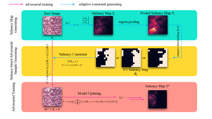
Figure 1: An overview of our proposed SCAAT. For each sample, we generate the region-averaged gradient-based saliency map whose resolution is same as the input image, then we select the regions to be perturbed in the adversarial training based on the proportion $q_{i}$. Then we involve the saliency constraints (i.e. high saliency pixels will not be perturbed) in adversarial sample generation and get the optimal adversarial sample using PGD-k [Madry et al.(2017)Madry, Makelov, Schmidt, Tsipras, and Vladu]. We further update model to improve its robustness to perturbations on those low-saliency features and adjust $q_{i}$ to get more suitable feature perturbing proportion for each instance.

2 Related Work

Interpretability

Interpretability research is critical to deep learning and is growing rapidly. Related work can be divided into three lines. The first line is about post-hoc explanation methods. Some gradient-based methods try to compute backpropagation for a modified gradient function, like [Baehrens et al.(2010)Baehrens, Schroeter, Harmeling, Kawanabe, Hansen, and Müller, Sundararajan et al.(2017)Sundararajan, Taly, and Yan, Smilkov et al.(2017)Smilkov, Thorat, Kim, Viégas, and Wattenberg, Shrikumar et al.(2017)Shrikumar, Greenside, and Kundaje, Lundberg and Lee(2017), Selvaraju et al.(2017)Selvaraju, Cogswell, Das, Vedantam, Parikh, and Batra]. And others [Zeiler and Fergus(2014), Suresh et al.(2017)Suresh, Hunt, Johnson, Celi, Szolovits, and Ghassemi, Ribeiro et al.(2016)Ribeiro, Singh, and Guestrin, Tonekaboni et al.(2020)Tonekaboni, Joshi, Campbell, Duvenaud, and Goldenberg], called perturbation-based methods, trying to perturb areas of the input and measure how much this changes the model output. The second line is about measure the reliability of interpretability methods [Adebayo et al.(2018)Adebayo, Gilmer, Muelly, Goodfellow, Hardt, and Kim, Adebayo et al.(2020)Adebayo, Muelly, Liccardi, and Kim, Ghorbani et al.(2019)Ghorbani, Abid, and Zou, Hooker et al.(2019)Hooker, Erhan, Kindermans, and Kim, Kindermans et al.(2019)Kindermans, Hooker, Adebayo, Alber, Schütt, Dähne, Erhan, and Kim, Petsiuk et al.(2018)Petsiuk, Das, and Saenko, Samek et al.(2016b)Samek, Binder, Montavon, Lapuschkin, and Müller, Tomsett et al.(2020b)Tomsett, Harborne, Chakraborty, Gurram, and Preece]. Other methods like [Ba and Caruana(2014), Frosst and Hinton(2017), Ismail et al.(2019)Ismail, Gunady, Pessoa, Corrada Bravo, and Feizi, Ross et al.(2017)Ross, Hughes, and Doshi-Velez, Wu et al.(2018)Wu, Hughes, Parbhoo, Zazzi, Roth, and Doshi-Velez] modifying neural architectures for better interpretability. Related to our work, [Ghaeini et al.(2019)Ghaeini, Fern, Shahbazi, and Tadepalli, Ross et al.(2017)Ross, Hughes, and Doshi-Velez, Ismail et al.(2021)Ismail, Corrada Bravo, and Feizi] incorporate explanations into the learning process.

Adversarial training

Adversarial samples are perturbed samples that are usually generated by adding small perturbations to the original samples that may mislead the neural network to make erroneous predictions [Szegedy et al.(2013)Szegedy, Zaremba, Sutskever, Bruna, Erhan, Goodfellow, and Fergus]. There are many popular methods to generate adversarial perturbations such as FGSM [Goodfellow et al.(2014)Goodfellow, Shlens, and Szegedy], PGD [Madry et al.(2017)Madry, Makelov, Schmidt, Tsipras, and Vladu], DeepFool [Moosavi-Dezfooli et al.(2016)Moosavi-Dezfooli, Fawzi, and Frossard], FreeAT [Shafahi et al.(2019)Shafahi, Najibi, Ghiasi, Xu, Dickerson, Studer, Davis, Taylor, and Goldstein] and YOPO [Zhang et al.(2019)Zhang, Zhang, Lu, Zhu, and Dong]. Based on these methods of adversarial sample generating, adversarial training has been widely used to make model robust to adversarial attacks [Pang et al.(2020)Pang, Yang, Dong, Su, and Zhu, Maini et al.(2020)Maini, Wong, and Kolter, Schott et al.(2018)Schott, Rauber, Bethge, and Brendel]. Different from those works that focus on improving the model robustness to adversarial attacks, our work aims to desensitize the model to perturbations on the irrelevant features only.

Input level perturbation

Input level perturbation during training has been previously explored. But most of these works try to improve performance or robustness rather than interpretability. [Wei et al.(2017)Wei, Feng, Liang, Cheng, Zhao, and Yan, Kumar Singh and Jae Lee(2017), Li et al.(2018)Li, Wu, Peng, Ernst, and Fu, Hou et al.(2018)Hou, Jiang, Wei, and Cheng] use attention maps to improve segmentation performance. And [Wang et al.(2019)Wang, Wu, Karanam, Peng, Singh, Liu, and Metaxas] use attention maps for training to improve performance of classfication. [DeVries and Taylor(2017)] improve the robustness and performance for convolutional neural networks. Related to our work, [Ismail et al.(2021)Ismail, Corrada Bravo, and Feizi] is the first work we know of improving model interpretability through input level perturbation in a self-supervised learning manner. Their work developed a pattern-fixed and interpretability-related regularization term under the guidance of saliency map, which differs from our method of generating adversarial samples systematically and adaptively to improve the model interpretability. Furthermore, our method significantly outperforms that of [Ismail et al.(2021)Ismail, Corrada Bravo, and Feizi] for both model interpretability and classification performance.

3 Method

3.1 Notation

First, let $\mathcal{D}=\left\{\left(\mathbf{X}_{i}\mathrm{,}\ {y_{i}}\right)\right\}_{i=1}^{N}$ denote the samples in training dataset, and each sample $\mathbf{X}_{i}=\left[x_{1},...,x_{n}\right]\in\mathbb{R}^{n}$ has $n$ features. In the classification task, the label can be formulated as $y_{i}\in\left\{1,2,...,N_{c}\right\}$, where $N_{c}$ denotes the class number. The neural network $f_{\theta}$ with learnable parameters $\theta$ takes $\mathbf{x}=\mathbf{X}_{i}\in\mathbb{R}^{n}$ as input, and $f_{\theta}(\mathbf{x}):\mathbb{R}^{n}\longrightarrow\mathbb{R}^{N_{c}}$ denotes that the network predicts the score of $N_{c}$ classes. The supervised learning objective is minimizing the cross-entropy loss $\mathcal{L}_{ce}$ between labels and predictions, which can be formulated as follows:

$$\min\limits_{\theta}\frac{1}{N}\sum\limits_{i=1}^{N}\mathcal{L}_{ce}(f_{\theta}(\mathbf{X}_{i}),\ y_{i})$$ (1)

Assume that the model takes $\mathbf{x}=\mathbf{X}_{i}$ as input with a classification label $y=y_{i}$, the gradient of the confidence of class $y$ with respect to $\mathbf{x}$ is given by $\nabla_{\mathbf{x}}f_{\theta}(\mathbf{x})\mid_{y}\ =\left\{g_{1},...,g_{n}\right\}\in\mathbb{R}^{n}$. Let $GSmap(f_{\theta},\mathbf{x},y)$ denote the absolute gradient-based saliency map $\left\{\left|g_{1}\right|,...,\left|g_{n}\right|\right\}$ for sample $\mathbf{x}$ of model $f_{\theta}$.

Let $S$ be a set of $s$ real numbers $\left\{a_{1},...,a_{s}\right\}$, $Lowest(S,q)$ outputs a set consisted of the indexes of those elements whose value is less than the bottom $q$-quantile value in the input set $S$, $i.e.$ $Lowest(S,q)=\left\{i\ |\ a_{i}<Quantile(S,q)\right\}$

For standard adversarial training methods [Bai et al.(2021)Bai, Luo, Zhao, Wen, and Wang], the most critical step is to find adversarial perturbation $\delta_{i}$ which can maximally confuse the model when being added to the clean sample $\mathbf{X}_{i}$, and the cross-entropy loss $\mathcal{L}_{ce}$ is often used as a measure of confusion. The objective of perturbation searching under an $\epsilon$-ball constraint can be formulated as follows:

$$\max\limits_{\left\|\delta_{i}\right\|_{\infty}\leq\epsilon}\frac{1}{N}\sum\limits_{i=1}^{N}\mathcal{L}_{ce}(f_{\theta}(\mathbf{X}_{i}+\delta_{i}),\ y_{i})$$ (2)

Given two probability distributions $P$ and $Q$ on probability space $\mathcal{X}$, the Kullback-Leibler (KL) divergence [Kullback and Leibler(1951)] from $P$ to $Q$ is defined as follows:

$$D_{KL}(P\ \left|\right|\ Q)={\textstyle\sum\limits_{x\in\mathcal{X}}}P(x)\cdot log_{2}\left(\frac{P(x)}{Q(x)}\right)$$ (3)

The Jensen–Shannon (JS) divergence [Lin(1991)] $D_{JS}$ is the symmetrical form of $D_{KL}$:

$$D_{JS}(P\ \left|\right|\ Q)=\frac{1}{2}D_{KL}(P\ \left|\right|\ Q)+\frac{1}{2}D_{KL}(Q\ \left|\right|\ P)$$ (4)

3.2 Saliency Constrained Adaptive Adversarial Training

To improve the sparsity and faithfulness of saliency map, the noise on irrelevant features in the saliency map must be eliminated [Ismail et al.(2021)Ismail, Corrada Bravo, and Feizi]. In other words, the model prediction should be robust to the small perturbations on irrelevant features while being sensitive to critical features, which makes the saliency map clearly indicate those features that are essential in model’s prediction process. We developed a novel adversarial-based learning objective to solve this problem.

First, we search for an optimal perturbation term $\delta_{i}^{\ast}\in\mathbb{R}^{n}$ for each sample $\mathbf{X}_{i}$ in the training set which maximizes the JS divergence [Lin(1991)] $D_{JS}$ between $f_{\theta}(\mathbf{X}_{i}+\delta_{i}^{\ast})$ and $f_{\theta}(\mathbf{X}_{i})$:

$$\delta_{i}^{\ast}=\mathop{\arg\max}\limits_{\delta_{i}}D_{JS}(f_{\theta}(\mathbf{X}_{i}+\delta_{i})\left|\right|f_{\theta}(\mathbf{X}_{i}))$$ (5)

Like standard adversarial training methods [Bai et al.(2021)Bai, Luo, Zhao, Wen, and Wang], the feasible perturbation $\delta_{i}$ is restricted to a small region controlled by $\epsilon$ since arbitrary perturbations may harm the model performance on clean samples. Additionally, we involve sample-specific saliency constraint for $\delta_{i}$ to prevent those features with high saliency values from being perturbed, thus the saliency map will be sparser and more faithful. The constraint for $\delta_{i}$ is formulated as follows:

$$\left\|\delta_{i}\right\|_{\infty}\leq\epsilon$$ (6)

and

$$\delta_{i}^{k}=0,\ k\notin Lowest(Smap(f_{\theta},\mathbf{X}_{i},y_{i}),\ q_{i})$$ (7)

For each sample $\mathbf{X}_{i}$, the value of $q_{i}$ determines what proportion of features in $\mathbf{X}_{i}$ will be perturbed, and it can be adjusted adaptively during the training process with an initialization value $q_{0}\in\left[0,1\right]$. The maximization problem above can be effectively solved by the PGD-k algorithm [Madry et al.(2017)Madry, Makelov, Schmidt, Tsipras, and Vladu].

The complete learning objective for our saliency constrained adversarial training is:

$$\min\limits_{\theta}\frac{1}{N}\sum\limits_{i=1}^{N}\Big{[} \mathcal{L}_{ce}(f_{\theta}(\mathbf{X}_{i}),\ y_{i})$$ (8)

$$+\lambda D_{JS}(f_{\theta}(\mathbf{X}_{i}+\delta_{i}^{\ast})\left|\right|f_{\theta}(\mathbf{X}_{i}))\Big{]}$$

where the $\delta_{i}^{\ast}$ is the optimal solution of the problem defined in formulation 5, and $\lambda$ is a hyper-parameter to balance the supervised loss and the divergence loss.

Algorithm 1 Saliency constrained adaptive adversarial training.

  Rquire: $N_{iter}$: Total training iterations

  Rquire: $PGD_{k}(f_{\theta},\mathbf{X}_{i},y_{i},\epsilon,IrreFeats_{i})$: The k-step PGD function [Madry et al.(2017)Madry, Makelov, Schmidt, Tsipras, and Vladu] to generate optimal adversarial perturbation $\delta_{i}^{\ast}$ in the constrained $\epsilon$-ball, guaranteeing $\delta_{i}^{k}=0,k\notin IrreFeats_{i}$

  Rquire: Feature perturbation proportions for each training sample: $q=\left\{q_{i}\right\}_{1}^{N}$ initialized by $q_{0}\in\left[0,1\right]$

  for $iter=1$ to $N_{iter}$ do

     Sample a batch $\left\{\left(\mathbf{X}_{i}\mathrm{,}\ {y_{i}}\right)\right\}_{i=1}^{N_{batch}}$ from the training set $\mathcal{D}$

     for $i=1$ to $N_{batch}$ do

        Generate saliency map

        $S_{i}=GSmap(f_{\theta},\mathbf{X}_{i},y_{i})$

        Select irrelevant features

        $IrreFeats_{i}=Lowest(S_{i},q_{i})$

        Generate adversarial samples

        $\mathbf{X}_{i}^{adv}=\mathbf{X}_{i}+PGD_{k}(f_{\theta},\mathbf{X}_{i},y_{i},\epsilon,IrreFeats_{i})$

        Compute the loss terms

        $L_{i}^{cls}=\mathcal{L}_{ce}(f_{\theta}(\mathbf{X}_{i}),\ y_{i})$

        $L_{i}^{adv}=D_{JS}(f_{\theta}(\mathbf{X}_{i}^{adv})\left|\right|f_{\theta}(\mathbf{X}_{i}))$

        Update $q_{i}$ using Algorithm 2

     end for

     Update the model parameters

     $\theta^{{}^{\prime}}=arg\min\limits_{\theta}\frac{1}{N^{batch}}\sum_{i=1}^{N^{batch}}\left(L^{cls}_{i}+\lambda L^{adv}_{i}\right)$

  end for

3.3 Adaptive Feature Perturbation Proportion

Intuitively, the ratio of irrelevant features varies across samples. For example, an image that is mostly background should have more irrelevant features than a dense one, which deserves more aggressive perturbing strategy (i.e. perturbing more low-saliency regions). In this sense, perturbing irrelevant features with fixed proportion for the whole dataset is sub-optimal while determining the suitable proportion for each training sample is more reasonable.

Our method optimizes perturbing proportion for each instance by adaptively adjusting the proportion $q_{i}$ for each sample $\mathbf{X}_{i}$ during training process. Before model training, the values of $\left\{q_{i}\right\}_{i=1}^{N}$ are initialized to the same empirically selected value $q_{0}\in\left[0,1\right]$, and will not be adjusted in the warm-up period. After that, we reduce $q_{i}$ by a step of $\gamma$ if the adversarial sample $\mathbf{X}_{adv}$ generated under the constraint of $q_{i}$ is misclassified by the model and vice versa. We believe that if small perturbations applied to $q_{i}$-proportion regions has crossed the model’s decision boundary and mislead the model to a wrong prediction, then the proportion should be reduced to protect model’s discrimination power.

Our training method is shown in Algorithm 1, and the details about how we update $q_{i}$ are in Algorithm 2.

Algorithm 2 $q$ updating algorithm

  Rquire: $i$: Index of sample, $iter$: Iteration index; $N^{warm-up}$: Warm-up iterations;

  Rquire: $q_{max},q_{min}$: Boundary values for $q$; $\gamma$: Discretization for $q$ searching.

  if $iter\leq N^{warm-up}$ then

     Set $q_{i}{}^{\prime}=q_{i}$

  else if $f_{\theta}(X_{i}^{adv})$ predicts as $y_{i}$ then

     Set $q_{i}{}^{\prime}=q_{i}+\gamma$

  else

     Set $q_{i}{}^{\prime}=q_{i}-\gamma$

  end if

  Set $q_{i}{}^{\prime\prime}=\min(\max(q_{i}{}^{\prime},\ q_{min}),\ q_{max})$

  return $q_{i}{}^{\prime\prime}$

4 Experiments

4.1 Datasets

To demonstrate our method can improve model interpretability across domains, we conduct experiments on the PCAM [Veeling et al.(2018)Veeling, Linmans, Winkens, Cohen, and Welling], CIFAR-10 [Krizhevsky et al.(2009)Krizhevsky, Hinton, et al.] and ImageNet-1k [Deng et al.(2009)Deng, Dong, Socher, Li, Li, and Fei-Fei] dataset. PCAM [Veeling et al.(2018)Veeling, Linmans, Winkens, Cohen, and Welling] is a dataset of pathological images which consists of 327680 color images ($96\times 96$ px) extracted from histopathologic scans of lymph node sections and has been generally used in the domain of computational pathology.

For each dataset, we train the model by SCAAT on ResNet-18 [He et al.(2016)He, Zhang, Ren, and Sun] and VGG-16 [Simonyan and Zisserman(2014)] then compare model interpretability and performance for regular training, previous method proposed by Ismail et al[Ismail et al.(2021)Ismail, Corrada Bravo, and Feizi] and our SCAAT.

4.2 Quality Evaluation for Saliency Map

Sparsity  Generally, a saliency map consists of pixel-wise scores that indicate relevant pixels for model decision. Good saliency maps should highlight relevant regions only, while sub-optimal saliency maps may have much noise and lack of sparsity. We select two metrics to evaluate the sparsity of a saliency map. One is entropy, and the other is compressed saliency map size in Kbyte. Faithfulness  Faithfulness is a measure that quantifies the extent to which the regions highlighted by a saliency map align with the true important regions for the given prediction. Compared with sparsity, faithfulness is a more comprehensive and important evaluation metric, because sparsity only evaluates the noise level of the saliency map, without considering how accurately the highlighted regions in the saliency map match the critical regions.

By following [Samek et al.(2016a)Samek, Binder, Montavon, Lapuschkin, and Müller, Tomsett et al.(2020a)Tomsett, Harborne, Chakraborty, Gurram, and Preece], we use AOPC to evaluate the saliency map faithfulness. Given a saliency map of a test sample, we iteratively perturb the regions (i.e. substitute them with random pixels) in the ascending order of region’s saliency score and feed model with these perturbed samples to get the prediction scores, thus we get a curve of prediction score decay versus feature perturbation steps. This curve is called LeRF perturbation curve [Tomsett et al.(2020a)Tomsett, Harborne, Chakraborty, Gurram, and Preece], where LeRF is short for Least Relevant First. In this sense, we compute the average of this curve which is denoted as AOPC${}_{\texttt{lerf}}$, and the lower value means a less noisy and more faithful saliency map.

Opposite to AOPC${}_{\texttt{lerf}}$, the method perturbing those regions with high saliency score first is called MoRF (i.e. Most Relevant First), and we combine these two metrics to a more comprehensive metric called relative AOPC [Samek et al.(2016a)Samek, Binder, Montavon, Lapuschkin, and Müller] (i.e. AOPC${}_{\texttt{rel}}$ $=$ AOPC${}_{\texttt{morf}}$ $/$ AOPC${}_{\texttt{lerf}}$) to get better estimation of faithfulness for a saliency map.

During evaluation, we perturb a significant part of each test image (20% regions) in 20 perturbation steps, and each perturbation step is repeated for 5 times.

4.3 Main Results

Table 1: Evaluation results of saliency map sparsity and faithfulness metrics. ($\uparrow$) indicates higher numbers are better, while ($\downarrow$) indicates lower numbers are better. We compare our model interpretability with regular trained model (i.e Rgl.) and the model trained with the method proposed by Ismail et al[Ismail et al.(2021)Ismail, Corrada Bravo, and Feizi] under different saliency visualization methods. Here the AOPC${}_{\texttt{lerf}}$ indicates how sensitive the model is to irrelevant features while AOPC${}_{\texttt{rel}}$ is a comprehensive metric for saliency map faithfulness and should be mainly focused. All models are ResNet-18 and the ’C’, ’P’ and ’I’ in the left column stand for the CIFAR-10, PCAM and ImageNet-1k dataset respectively.

	Metric	Vallina Grad			Smooth Grad			Integrated Grad
		Rgl.	Ismail	Ours	Rgl.	Ismail	Ours	Rgl.	Ismail	Ours
C	Sal. Entropy $\downarrow$	5.89	5.60	4.69	5.86	5.69	4.71	5.56	5.40	4.34
	Sal. Size (Kbyte) $\downarrow$	3.30	2.93	1.95	3.14	2.91	1.92	2.84	2.63	1.80
	AOPC${}_{\texttt{lerf}}$$\downarrow$ ($10^{-3}$)	220	14.6	0.18	180	11.7	0.32	220	38.4	0.36
	AOPC${}_{\texttt{rel}}$ $\uparrow$	2.18	17.1	960	2.72	22.2	917	2.18	6.25	801
P	Sal. Entropy $\downarrow$	5.61	5.30	4.56	5.60	5.43	4.54	4.93	4.72	4.43
	Sal. Size (Kbyte) $\downarrow$	2.48	2.34	1.61	2.45	2.33	1.61	2.23	2.04	1.52
	AOPC${}_{\texttt{lerf}}$$\downarrow$ ($10^{-3}$)	3.20	6.25	0.23	2.89	6.29	0.23	8.94	7.65	0.21
	AOPC${}_{\texttt{rel}}$ $\uparrow$	78.1	38.4	1030	90.0	38.1	982	24.6	28.8	938
I	Sal. Entropy $\downarrow$	5.49	5.21	4.45	5.12	5.01	4.23	4.98	4.85	4.15
	Sal. Size (Kbyte) $\downarrow$	13.2	11.9	7.12	12.9	12.7	6.94	12.8	12.4	6.80
	AOPC${}_{\texttt{lerf}}$$\downarrow$ ($10^{-3}$)	85.2	42.1	0.98	72.5	56.9	0.93	43.2	21.8	1.21
	AOPC${}_{\texttt{rel}}$ $\uparrow$	3.84	5.13	321	4.66	6.56	346	4.21	7.93	305

We evaluate the model performance and the quality of our model’s saliency map generated by different saliency methods and compare them with that of the baseline and of [Ismail et al.(2021)Ismail, Corrada Bravo, and Feizi]. Table 1 shows the comparison of saliency map quality with the baseline and the model proposed by Ismail et al[Ismail et al.(2021)Ismail, Corrada Bravo, and Feizi]. For all of the listed saliency methods and evaluation metrics, our SCAAT beats baseline and Ismail et al[Ismail et al.(2021)Ismail, Corrada Bravo, and Feizi] under multiple evaluation metrics for both natural and pathological images. For example, on the ImageNet-1k [Deng et al.(2009)Deng, Dong, Socher, Li, Li, and Fei-Fei] dataset, the AOPC${}_{\texttt{lerf}}$ of gradient-based saliency map is decreased from $8.52\times 10^{-2}$ of baseline and $4.21\times 10^{-2}$ of [Ismail et al.(2021)Ismail, Corrada Bravo, and Feizi] to $9.8\times 10^{-4}$, which is reduced over one order of magnitude. Figure 2(a) shows the saliency map entropy distribution of our model and the baseline for all test samples. Figure 2(b) shows the comparison between the perturbation curves. Specifically, when we perturbs 20% low-saliency features of the input samples in ImageNet-1k [Deng et al.(2009)Deng, Dong, Socher, Li, Li, and Fei-Fei], the average prediction score decay of baseline model is at the level of $10^{-2}$ while $10^{-4}$ for our SCAAT.

In addition to model interpretability, Table 2 compares the performance and interpretability with our method and others. Our method with adaptive $q$ achieves comparable performance to the baseline model and higher than [Ismail et al.(2021)Ismail, Corrada Bravo, and Feizi] with a significant margin. Specifically, our method performs even better than the baseline model on discrimination power for pathological images.

Figure 3(a) visualizes the saliency map of the ResNet-18 [He et al.(2016)He, Zhang, Ren, and Sun] model trained by SCAAT and baseline method on both PCAM [Veeling et al.(2018)Veeling, Linmans, Winkens, Cohen, and Welling] and ImageNet-1k [Deng et al.(2009)Deng, Dong, Socher, Li, Li, and Fei-Fei] dataset. Obviously our method enhances the model’s sensitivity to critical features while suppressing the noise on irrelevant features, so the saliency map looks more sparse and accurately indicates the critical features. Figure 3(b) shows the representative training samples in PCAM [Veeling et al.(2018)Veeling, Linmans, Winkens, Cohen, and Welling] of different $q$ which are adjusted during the process of our adaptive adversarial training. Obviously the images with more uncritical regions will be assigned larger $q$ values adaptively in the training process, which means we can perturb more their irrelevant features to get cleaner saliency map without making the model misclassify them.

Table 2: Performance comparison. We test the performance of baseline methods and ours under fixed or adaptive saliency constraint. The metric of performance is top-1 ACC for CIFAR-10 [Krizhevsky et al.(2009)Krizhevsky, Hinton, et al.] and ImageNet-1k [Deng et al.(2009)Deng, Dong, Socher, Li, Li, and Fei-Fei] while AUC for PCAM [Veeling et al.(2018)Veeling, Linmans, Winkens, Cohen, and Welling], and Intp. indicates the AOPC${}_{\texttt{rel}}$ of gradient-based saliency map. The models trained by our method have comparable performance with baseline while the interpretability is significantly improved.

Dataset	Method	ResNet-18		VGG-16
		Perf.	Intp.	Perf.	Intp.
CIFAR-10	Regular	0.910	2.18	0.904	2.35
	Ismail	0.892	17.1	0.889	15.2
	Ours (fixed $q$)	0.890	871	0.893	896
	Ours (adpt. $q$)	0.905	960	0.901	921
PCAM	Regular	0.928	78.1	0.935	85.3
	Ismail	0.911	38.4	0.929	78.4
	Ours (fixed $q$)	0.926	987	0.931	801
	Ours (adpt. $q$)	0.933	1030	0.939	956
ImageNet-1k	Regular	0.687	3.84	0.744	4.29
	Ismail	0.653	5.13	0.684	6.05
	Ours (fixed $q$)	0.671	215	0.721	266
	Ours (adpt. $q$)	0.682	321	0.738	368

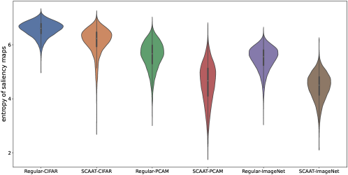
(a) Entropy distributions.

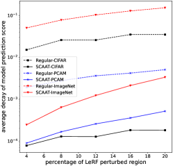
(b) Perturbation curves.

Figure 2: (a) Comparison of saliency map entropy distributions. (b) Comparison of the confidence-decay curve.

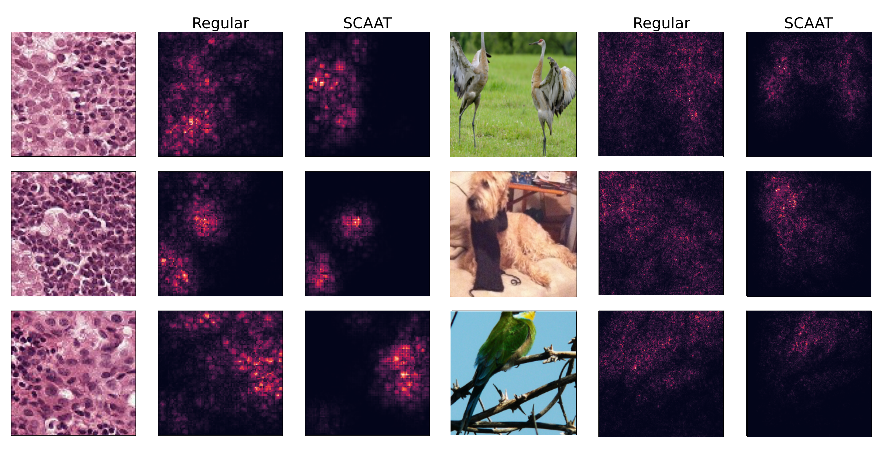
(a) Saliency map comparison.

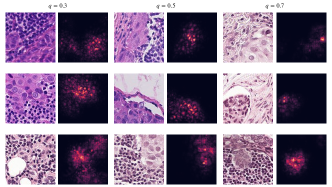
(b) Samples of different $q$ values.

Figure 3: (a) Visualizations of saliency maps of baseline model and ours. Left pane is for PCAM and right pane is for ImageNet-1k. (b) Visualizations of training samples and their saliency maps with values of $q$ which are searched in the training process.

Adaptive adversarial training is the core module of SCAAT to improve the model’s interpretability. Thus we did a lot of experiments for the adaptive $q$-selecting algorithm, the loss function of divergence, and the searching radius for perturbations. These detailed results are shown in the supplementary materials.

4.4 Training Efficiency

The extra training cost for our SCAAT mainly comes from adversarial sample generation, which just requires several back-propagation steps and depends on the searching algorithm. The default step is set to 4 in our work, which makes the training time about 2.5$\times$ longer than regular training. Additionally, FGSM[Goodfellow et al.(2014)Goodfellow, Shlens, and Szegedy] fast searching requires only one extra gradient step, leading to slight interpretability sacrifice but significant efficiency gains (see the last row in Table 3). There is a trade-off between quality of adversarial samples and the computational efficiency.

Towards the computational efficiency, we simply determine irrelevant features in each image according to the saliency map of vallina gradients. Despite requiring several extra back-propagation steps, we also experimented with Smooth Grad [Smilkov et al.(2017)Smilkov, Thorat, Kim, Viégas, and Wattenberg], which more precisely indicates uncritical features then prevents the model from being desensitised to the critical features. The performance can be further improved by introducing this more advanced saliency method, but the computational overhead will be greatly increased during training.

Table 3: Efficiency Comparison. We evaluate the extra training cost of our method. The Gini Index proposed in [Chalasani et al.(2020)Chalasani, Chen, Chowdhury, Wu, and Jha] measures the sparsity of saliency maps.

Dataset	Method	Acc(%)	Gini Index $\uparrow$	Time
ImageNet-1k	Regular	68.7$\pm$0.1	0.455	1.0$\times$
	Ours (PGD-4)	68.3$\pm$0.2	0.601	2.5$\times$
	Ours (FGSM)	68.4$\pm$0.2	0.578	1.4$\times$

5 Conclusion

In this work, we focus on improving interpretability of deep neural networks by denoising the saliency maps of a model. We proposed a model-agnostic adversary-based training method using saliency map as constraints to desensitize a model to irrelevant features. Motivated by the observation that the ratio of irrelevant features varies across training samples, the proposed method iteratively estimates the ratio of irrelevant features in a saliency map for further desensitizing perturbation, according to the dynamic impact on the model. Experiments showed our proposed training method achieves significant improvement on the quality of saliency map for both natural and pathological images without sacrifying model performance.

6 Acknowledgement

This research was supported in part by the NIFDC Key Technology Research Grant (GJJS-2022-3-1). We thank Qiuchuan Liang for doing some data processing work.

References

- [Adebayo et al.(2018)Adebayo, Gilmer, Muelly, Goodfellow, Hardt, and Kim] Julius Adebayo, Justin Gilmer, Michael Muelly, Ian Goodfellow, Moritz Hardt, and Been Kim. Sanity checks for saliency maps. Advances in neural information processing systems, 31, 2018.
- [Adebayo et al.(2020)Adebayo, Muelly, Liccardi, and Kim] Julius Adebayo, Michael Muelly, Ilaria Liccardi, and Been Kim. Debugging tests for model explanations. arXiv preprint arXiv:2011.05429, 2020.
- [Ba and Caruana(2014)] Jimmy Ba and Rich Caruana. Do deep nets really need to be deep? Advances in neural information processing systems, 27, 2014.
- [Bach et al.(2015)Bach, Binder, Montavon, Klauschen, Müller, and Samek] Sebastian Bach, Alexander Binder, Grégoire Montavon, Frederick Klauschen, Klaus-Robert Müller, and Wojciech Samek. On pixel-wise explanations for non-linear classifier decisions by layer-wise relevance propagation. PloS one, 10(7):e0130140, 2015.
- [Baehrens et al.(2010)Baehrens, Schroeter, Harmeling, Kawanabe, Hansen, and Müller] David Baehrens, Timon Schroeter, Stefan Harmeling, Motoaki Kawanabe, Katja Hansen, and Klaus-Robert Müller. How to explain individual classification decisions. The Journal of Machine Learning Research, 11:1803–1831, 2010.
- [Bai et al.(2021)Bai, Luo, Zhao, Wen, and Wang] Tao Bai, Jinqi Luo, Jun Zhao, Bihan Wen, and Qian Wang. Recent advances in adversarial training for adversarial robustness. arXiv preprint arXiv:2102.01356, 2021.
- [Chalasani et al.(2020)Chalasani, Chen, Chowdhury, Wu, and Jha] Prasad Chalasani, Jiefeng Chen, Amrita Roy Chowdhury, Xi Wu, and Somesh Jha. Concise explanations of neural networks using adversarial training. In International Conference on Machine Learning, pages 1383–1391. PMLR, 2020.
- [Deng et al.(2009)Deng, Dong, Socher, Li, Li, and Fei-Fei] Jia Deng, Wei Dong, Richard Socher, Li-Jia Li, Kai Li, and Li Fei-Fei. Imagenet: A large-scale hierarchical image database. In 2009 IEEE conference on computer vision and pattern recognition, pages 248–255. Ieee, 2009.
- [DeVries and Taylor(2017)] Terrance DeVries and Graham W Taylor. Improved regularization of convolutional neural networks with cutout. arXiv preprint arXiv:1708.04552, 2017.
- [Frosst and Hinton(2017)] Nicholas Frosst and Geoffrey Hinton. Distilling a neural network into a soft decision tree. arXiv preprint arXiv:1711.09784, 2017.
- [Ghaeini et al.(2019)Ghaeini, Fern, Shahbazi, and Tadepalli] Reza Ghaeini, Xiaoli Z Fern, Hamed Shahbazi, and Prasad Tadepalli. Saliency learning: Teaching the model where to pay attention. arXiv preprint arXiv:1902.08649, 2019.
- [Ghorbani et al.(2019)Ghorbani, Abid, and Zou] Amirata Ghorbani, Abubakar Abid, and James Zou. Interpretation of neural networks is fragile. In Proceedings of the AAAI conference on artificial intelligence, volume 33, pages 3681–3688, 2019.
- [Goodfellow et al.(2014)Goodfellow, Shlens, and Szegedy] Ian J Goodfellow, Jonathon Shlens, and Christian Szegedy. Explaining and harnessing adversarial examples. arXiv preprint arXiv:1412.6572, 2014.
- [He et al.(2016)He, Zhang, Ren, and Sun] Kaiming He, Xiangyu Zhang, Shaoqing Ren, and Jian Sun. Deep residual learning for image recognition. In Proceedings of the IEEE conference on computer vision and pattern recognition, pages 770–778, 2016.
- [Hooker et al.(2019)Hooker, Erhan, Kindermans, and Kim] Sara Hooker, Dumitru Erhan, Pieter-Jan Kindermans, and Been Kim. A benchmark for interpretability methods in deep neural networks. Advances in neural information processing systems, 32, 2019.
- [Hou et al.(2018)Hou, Jiang, Wei, and Cheng] Qibin Hou, PengTao Jiang, Yunchao Wei, and Ming-Ming Cheng. Self-erasing network for integral object attention. Advances in Neural Information Processing Systems, 31, 2018.
- [Huang et al.(2022)Huang, Liu, Zhang, Zhang, Xu, Wang, and Liu] Peixiang Huang, Li Liu, Renrui Zhang, Song Zhang, Xinli Xu, Baichao Wang, and Guoyi Liu. Tig-bev: Multi-view bev 3d object detection via target inner-geometry learning, 2022.
- [Huang et al.(2023)Huang, Zhang, Gan, Xu, Zhu, Qin, Guo, Jiang, and Luo] Peixiang Huang, Songtao Zhang, Yulu Gan, Rui Xu, Rongqi Zhu, Wenkang Qin, Limei Guo, Shan Jiang, and Lin Luo. Assessing and enhancing robustness of deep learning models with corruption emulation in digital pathology, 2023.
- [Ismail et al.(2019)Ismail, Gunady, Pessoa, Corrada Bravo, and Feizi] Aya Abdelsalam Ismail, Mohamed Gunady, Luiz Pessoa, Hector Corrada Bravo, and Soheil Feizi. Input-cell attention reduces vanishing saliency of recurrent neural networks. Advances in Neural Information Processing Systems, 32, 2019.
- [Ismail et al.(2021)Ismail, Corrada Bravo, and Feizi] Aya Abdelsalam Ismail, Hector Corrada Bravo, and Soheil Feizi. Improving deep learning interpretability by saliency guided training. Advances in Neural Information Processing Systems, 34:26726–26739, 2021.
- [Kindermans et al.(2019)Kindermans, Hooker, Adebayo, Alber, Schütt, Dähne, Erhan, and Kim] Pieter-Jan Kindermans, Sara Hooker, Julius Adebayo, Maximilian Alber, Kristof T Schütt, Sven Dähne, Dumitru Erhan, and Been Kim. The (un) reliability of saliency methods. Explainable AI: Interpreting, explaining and visualizing deep learning, pages 267–280, 2019.
- [Krizhevsky et al.(2009)Krizhevsky, Hinton, et al.] Alex Krizhevsky, Geoffrey Hinton, et al. Learning multiple layers of features from tiny images. 2009.
- [Kullback and Leibler(1951)] Solomon Kullback and Richard A Leibler. On information and sufficiency. The annals of mathematical statistics, 22(1):79–86, 1951.
- [Kumar Singh and Jae Lee(2017)] Krishna Kumar Singh and Yong Jae Lee. Hide-and-seek: Forcing a network to be meticulous for weakly-supervised object and action localization. In Proceedings of the IEEE International Conference on Computer Vision, pages 3524–3533, 2017.
- [Li et al.(2018)Li, Wu, Peng, Ernst, and Fu] Kunpeng Li, Ziyan Wu, Kuan-Chuan Peng, Jan Ernst, and Yun Fu. Tell me where to look: Guided attention inference network. In Proceedings of the IEEE Conference on Computer Vision and Pattern Recognition, pages 9215–9223, 2018.
- [Lin(1991)] Jianhua Lin. Divergence measures based on the shannon entropy. IEEE Transactions on Information theory, 37(1):145–151, 1991.
- [Lundberg and Lee(2017)] Scott M Lundberg and Su-In Lee. A unified approach to interpreting model predictions. Advances in neural information processing systems, 30, 2017.
- [Ma et al.(2023)Ma, Zhang, Lu, and Luo] Tao Ma, Chao Zhang, Min Lu, and Lin Luo. Agmdt: Virtual staining of renal histology images with adjacency-guided multi-domain transfer, 2023.
- [Madry et al.(2017)Madry, Makelov, Schmidt, Tsipras, and Vladu] Aleksander Madry, Aleksandar Makelov, Ludwig Schmidt, Dimitris Tsipras, and Adrian Vladu. Towards deep learning models resistant to adversarial attacks. arXiv preprint arXiv:1706.06083, 2017.
- [Maini et al.(2020)Maini, Wong, and Kolter] Pratyush Maini, Eric Wong, and Zico Kolter. Adversarial robustness against the union of multiple perturbation models. In International Conference on Machine Learning, pages 6640–6650. PMLR, 2020.
- [Moosavi-Dezfooli et al.(2016)Moosavi-Dezfooli, Fawzi, and Frossard] Seyed-Mohsen Moosavi-Dezfooli, Alhussein Fawzi, and Pascal Frossard. Deepfool: a simple and accurate method to fool deep neural networks. In Proceedings of the IEEE conference on computer vision and pattern recognition, pages 2574–2582, 2016.
- [Pang et al.(2020)Pang, Yang, Dong, Su, and Zhu] Tianyu Pang, Xiao Yang, Yinpeng Dong, Hang Su, and Jun Zhu. Bag of tricks for adversarial training. arXiv preprint arXiv:2010.00467, 2020.
- [Petsiuk et al.(2018)Petsiuk, Das, and Saenko] Vitali Petsiuk, Abir Das, and Kate Saenko. Rise: Randomized input sampling for explanation of black-box models. arXiv preprint arXiv:1806.07421, 2018.
- [Preuer et al.(2019)Preuer, Klambauer, Rippmann, Hochreiter, and Unterthiner] Kristina Preuer, Günter Klambauer, Friedrich Rippmann, Sepp Hochreiter, and Thomas Unterthiner. Interpretable deep learning in drug discovery, 2019.
- [Qin et al.(2022)Qin, Xu, Jiang, Jiang, and Luo] Wenkang Qin, Rui Xu, Shan Jiang, Tingting Jiang, and Lin Luo. Pathtr: Context-aware memory transformer for tumor localization in gigapixel pathology images. In Proceedings of the Asian Conference on Computer Vision, pages 3603–3619, 2022.
- [Qin et al.(2023)Qin, Xu, Huang, Wu, Zhang, and Luo] Wenkang Qin, Rui Xu, Peixiang Huang, Xiaomin Wu, Heyu Zhang, and Lin Luo. What a whole slide image can tell? subtype-guided masked transformer for pathological image captioning. arXiv preprint arXiv:2310.20607, 2023.
- [Ribeiro et al.(2016)Ribeiro, Singh, and Guestrin] Marco Tulio Ribeiro, Sameer Singh, and Carlos Guestrin. " why should i trust you?" explaining the predictions of any classifier. In Proceedings of the 22nd ACM SIGKDD international conference on knowledge discovery and data mining, pages 1135–1144, 2016.
- [Ross et al.(2017)Ross, Hughes, and Doshi-Velez] Andrew Slavin Ross, Michael C Hughes, and Finale Doshi-Velez. Right for the right reasons: Training differentiable models by constraining their explanations. arXiv preprint arXiv:1703.03717, 2017.
- [Samek et al.(2016a)Samek, Binder, Montavon, Lapuschkin, and Müller] Wojciech Samek, Alexander Binder, Grégoire Montavon, Sebastian Lapuschkin, and Klaus-Robert Müller. Evaluating the visualization of what a deep neural network has learned. IEEE transactions on neural networks and learning systems, 28(11):2660–2673, 2016a.
- [Samek et al.(2016b)Samek, Binder, Montavon, Lapuschkin, and Müller] Wojciech Samek, Alexander Binder, Grégoire Montavon, Sebastian Lapuschkin, and Klaus-Robert Müller. Evaluating the visualization of what a deep neural network has learned. IEEE transactions on neural networks and learning systems, 28(11):2660–2673, 2016b.
- [Schott et al.(2018)Schott, Rauber, Bethge, and Brendel] Lukas Schott, Jonas Rauber, Matthias Bethge, and Wieland Brendel. Towards the first adversarially robust neural network model on mnist. arXiv preprint arXiv:1805.09190, 2018.
- [Selvaraju et al.(2017)Selvaraju, Cogswell, Das, Vedantam, Parikh, and Batra] Ramprasaath R Selvaraju, Michael Cogswell, Abhishek Das, Ramakrishna Vedantam, Devi Parikh, and Dhruv Batra. Grad-cam: Visual explanations from deep networks via gradient-based localization. In Proceedings of the IEEE international conference on computer vision, pages 618–626, 2017.
- [Shafahi et al.(2019)Shafahi, Najibi, Ghiasi, Xu, Dickerson, Studer, Davis, Taylor, and Goldstein] Ali Shafahi, Mahyar Najibi, Mohammad Amin Ghiasi, Zheng Xu, John Dickerson, Christoph Studer, Larry S Davis, Gavin Taylor, and Tom Goldstein. Adversarial training for free! Advances in Neural Information Processing Systems, 32, 2019.
- [Shrikumar et al.(2017)Shrikumar, Greenside, and Kundaje] Avanti Shrikumar, Peyton Greenside, and Anshul Kundaje. Learning important features through propagating activation differences. In International conference on machine learning, pages 3145–3153. PMLR, 2017.
- [Simonyan and Zisserman(2014)] Karen Simonyan and Andrew Zisserman. Very deep convolutional networks for large-scale image recognition. arXiv preprint arXiv:1409.1556, 2014.
- [Simonyan et al.(2013)Simonyan, Vedaldi, and Zisserman] Karen Simonyan, Andrea Vedaldi, and Andrew Zisserman. Deep inside convolutional networks: Visualising image classification models and saliency maps. arXiv preprint arXiv:1312.6034, 2013.
- [Smilkov et al.(2017)Smilkov, Thorat, Kim, Viégas, and Wattenberg] Daniel Smilkov, Nikhil Thorat, Been Kim, Fernanda Viégas, and Martin Wattenberg. Smoothgrad: removing noise by adding noise. arXiv preprint arXiv:1706.03825, 2017.
- [Sundararajan et al.(2017)Sundararajan, Taly, and Yan] Mukund Sundararajan, Ankur Taly, and Qiqi Yan. Axiomatic attribution for deep networks. In International conference on machine learning, pages 3319–3328. PMLR, 2017.
- [Suresh et al.(2017)Suresh, Hunt, Johnson, Celi, Szolovits, and Ghassemi] Harini Suresh, Nathan Hunt, Alistair Johnson, Leo Anthony Celi, Peter Szolovits, and Marzyeh Ghassemi. Clinical intervention prediction and understanding using deep networks. arXiv preprint arXiv:1705.08498, 2017.
- [Szegedy et al.(2013)Szegedy, Zaremba, Sutskever, Bruna, Erhan, Goodfellow, and Fergus] Christian Szegedy, Wojciech Zaremba, Ilya Sutskever, Joan Bruna, Dumitru Erhan, Ian Goodfellow, and Rob Fergus. Intriguing properties of neural networks. arXiv preprint arXiv:1312.6199, 2013.
- [Tomsett et al.(2020a)Tomsett, Harborne, Chakraborty, Gurram, and Preece] Richard Tomsett, Dan Harborne, Supriyo Chakraborty, Prudhvi Gurram, and Alun Preece. Sanity checks for saliency metrics. In Proceedings of the AAAI conference on artificial intelligence, volume 34, pages 6021–6029, 2020a.
- [Tomsett et al.(2020b)Tomsett, Harborne, Chakraborty, Gurram, and Preece] Richard Tomsett, Dan Harborne, Supriyo Chakraborty, Prudhvi Gurram, and Alun Preece. Sanity checks for saliency metrics. In Proceedings of the AAAI conference on artificial intelligence, volume 34, pages 6021–6029, 2020b.
- [Tonekaboni et al.(2020)Tonekaboni, Joshi, Campbell, Duvenaud, and Goldenberg] Sana Tonekaboni, Shalmali Joshi, Kieran Campbell, David K Duvenaud, and Anna Goldenberg. What went wrong and when? instance-wise feature importance for time-series black-box models. Advances in Neural Information Processing Systems, 33:799–809, 2020.
- [Veeling et al.(2018)Veeling, Linmans, Winkens, Cohen, and Welling] Bastiaan S Veeling, Jasper Linmans, Jim Winkens, Taco Cohen, and Max Welling. Rotation equivariant CNNs for digital pathology. June 2018.
- [Wang et al.(2019)Wang, Wu, Karanam, Peng, Singh, Liu, and Metaxas] Lezi Wang, Ziyan Wu, Srikrishna Karanam, Kuan-Chuan Peng, Rajat Vikram Singh, Bo Liu, and Dimitris N Metaxas. Sharpen focus: Learning with attention separability and consistency. In Proceedings of the IEEE/CVF International Conference on Computer Vision, pages 512–521, 2019.
- [Wei et al.(2017)Wei, Feng, Liang, Cheng, Zhao, and Yan] Yunchao Wei, Jiashi Feng, Xiaodan Liang, Ming-Ming Cheng, Yao Zhao, and Shuicheng Yan. Object region mining with adversarial erasing: A simple classification to semantic segmentation approach. In Proceedings of the IEEE conference on computer vision and pattern recognition, pages 1568–1576, 2017.
- [Wu et al.(2018)Wu, Hughes, Parbhoo, Zazzi, Roth, and Doshi-Velez] Mike Wu, Michael Hughes, Sonali Parbhoo, Maurizio Zazzi, Volker Roth, and Finale Doshi-Velez. Beyond sparsity: Tree regularization of deep models for interpretability. In Proceedings of the AAAI conference on artificial intelligence, volume 32, 2018.
- [Yang et al.(2023)Yang, Xu, Guo, Huang, Chen, Ding, Wang, and Zhou] Cheng Yang, Rui Xu, Ye Guo, Peixiang Huang, Yiru Chen, Wenkui Ding, Zhongyuan Wang, and Hong Zhou. Improving vision-and-language reasoning via spatial relations modeling, 2023.
- [Zeiler and Fergus(2014)] Matthew D Zeiler and Rob Fergus. Visualizing and understanding convolutional networks. In Computer Vision–ECCV 2014: 13th European Conference, Zurich, Switzerland, September 6-12, 2014, Proceedings, Part I 13, pages 818–833. Springer, 2014.
- [Zhang et al.(2019)Zhang, Zhang, Lu, Zhu, and Dong] Dinghuai Zhang, Tianyuan Zhang, Yiping Lu, Zhanxing Zhu, and Bin Dong. You only propagate once: Accelerating adversarial training via maximal principle. Advances in Neural Information Processing Systems, 32, 2019.
- [Zhou et al.(2016)Zhou, Khosla, Lapedriza, Oliva, and Torralba] Bolei Zhou, Aditya Khosla, Agata Lapedriza, Aude Oliva, and Antonio Torralba. Learning deep features for discriminative localization. In Proceedings of the IEEE conference on computer vision and pattern recognition, pages 2921–2929, 2016.