Vector Approximate Survey Propagation for Model-Mismatched Estimation (Or: How to Achieve Kabashima’s 1RSB Prediction)

Abstract

For approximate inference in high-dimensional generalized linear models (GLMs), the performance of an estimator may significantly degrade when mismatch exists between the postulated model and the ground truth. In mismatched GLMs with rotation-invariant measurement matrices, Kabashima et al. proved vector approximate message passing (VAMP) computes exactly the optimal estimator if the replica symmetry (RS) ansatz is valid, but it becomes inappropriate if RS breaking (RSB) appears. Although the one-step RSB (1RSB) saddle point equations were given for the optimal estimator, the question remains: how to achieve the 1RSB prediction? This paper answers the question by proposing a new algorithm, vector approximate survey propagation (VASP). VASP derives from a reformulation of Kabashima’s extremum conditions, which later links the theoretical equations to survey propagation in vector form and finally the algorithm. VASP has a complexity as low as VAMP, while embracing VAMP as a special case. The SE derived for VASP can capture precisely the per-iteration behavior of the simulated algorithm, and the SE’s fixed point equations perfectly match Kabashima’s 1RSB prediction, which indicates VASP can achieve the optimal performance even in a model-mismatched setting with 1RSB. Simulation results confirm VASP outperforms many state-of-the-art algorithms.

I Introduction

In this paper, we study the recovery of a high-dimensional input signal from the output of a generalized linear model (GLM), where model mismatch exists. As shown in Fig. 1, the input signal in the generation phase is $\bm{x}_{0}\in\mathbb{R}^{N\times 1}$, and the observation is $\bm{y}\in\mathbb{R}^{M\times 1}$, where $\bm{H}\in\mathbb{R}^{M\times N}$ is the deterministic measurement matrix. The input-output relationship of the GLM is characterized by:

$$\bm{y}\sim p(\bm{y}|\bm{z}_{0})=\prod_{a=1}^{M}p(y_{a}|z_{0,a}),\quad\bm{z}_{0}\triangleq\bm{H}\bm{x}_{0},$$ (1)

$$\bm{x}\sim p(\bm{x}_{0})=\prod_{i=1}^{N}p(x_{0,i}).$$ (2)

In the inference phase, the estimator relies on a postulated (mismatched) prior $q(\bm{x}_{0})=\prod_{i=1}^{N}q(x_{0,i})$ and a postulated likelihood $q(\bm{y}|\bm{z}_{0})=\prod_{a=1}^{M}q(y_{a}|z_{0,a})$ to recover the input in a criterion of minimum mean square error (MMSE) or maximum a posteriori (MAP), i.e., [1, 2]:

$$\hat{\bm{x}}_{0}= \int{\mathsf{d}\bm{z}_{0}\mathsf{d}\bm{x}_{0}}\,q(\bm{z}_{0},\bm{x}_{0},\kappa)\bm{x}_{0},$$ (3)

$$q(\bm{z}_{0},\bm{x}_{0},\kappa)= \frac{1}{\mathsf{const}}q^{\kappa}(\bm{y}|\bm{z}_{0})\delta(\bm{z}_{0}-\bm{H}\bm{x}_{0})q^{\kappa}(\bm{x}_{0}),$$ (4)

where $\hat{\bm{x}}_{0}$ is the MMSE estimate if $\kappa=1$, and the MAP if $\kappa\to+\infty$. Throughout this paper, we consider exclusively the large system limit, i.e., $M\rightarrow\infty$ and $N\rightarrow\infty$, with a fixed and bounded $\alpha\triangleq M/N$. In the large system limit, computing exactly the Bayes-optimal estimator (3) requires the integration over all variables, which can be in the millions or billions for some applications. Exact inference is therefore intractable, and approximation is needed.

The central idea of approximate inference is to approximate the posterior by a simpler distribution. EP [3, 4] is one such inference method: it minimizes the Kullback-Leibler divergence between the posterior and the approximating distribution (Gaussian), thus enjoying high computation efficiency. Refinements of EP have since been proposed, which includes a generalization to the GLM [5], to the multi-layer problem [6], and to a decentralized implementation [7] among many others. Another prevailing approximate method is AMP [8, 9], a parameterized and simplified sum-product algorithm of the loopy belief propagation [10] applied to dense networks. The popularity of AMP stems from a unique attractive feature: under mild model assumptions, the AMP performance in the high-dimensional limit is precisely characterized by a concise deterministic recursion called state evolution (SE) [11], and using SE, AMP provably achieves the Bayes-optimal performance in a number of settings [12]. Motivated by AMP, a series of refinements has been proposed, which includes an extension to GLM [2], to bilinear setup [13, 14], and to ill-condition handling [15, 16] among many others. As pointed out in [16], two AMP refinements, OAMP [17] and VAMP [18], are closely connected with EP [3, 4], and in certain cases, the three are equivalent. More connections between AMP and EP families can be found in [19, 20] among others.

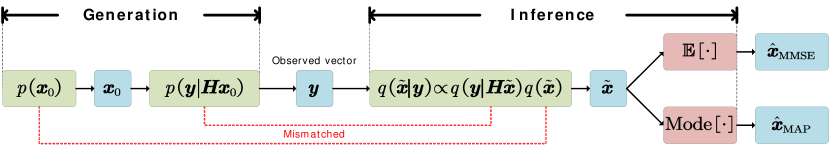
Figure 1: Estimation in generalized linear model with mismatch

However, the above results all rely on a key assumption that the estimator perfectly knows the prior and the likelihood distributions used in the generation phase. In case a model mismatch occurs, i.e., the prior and/or the likelihood postulated by the estimator are not equal to the ground truth, a situation frequently encountered in practice, many (if not all) the above results are not applicable. Currently, only a few results are available on the approximate inference in a model-mismatch setting. In [21], Antenucci et al. pointed out that when there is a model mismatch between the generation and the inference, the performance of Low-RAMP [22] (a refinement of AMP) degrades rapidly in terms of MSE and convergence. They thereby put forward a new algorithm for approximate inference called approximate survey propagation (ASP), which took into account the glassy nature of the low-rank matrix estimation problem. Compared with Low-RAMP, the ASP converges in a larger regime and can reach lower MSEs. More importantly, its SE can reproduce the one-step replica symmetry breaking (1RSB) saddle point equations, well-known in physics of disordered systems. In [23], Lucibello et al. observed that generalized AMP (GAMP)[2] is significantly degraded whenever there is a mismatch in the model. They proposed a new algorithm, generalized ASP (GASP) [23], for solving the mismatched GLM problem. The GASP generally outperforms GAMP and approaches the Bayesian optimal performance. The SE of GASP can exactly characterize the algorithm’s dynamics in large system limits. However, the derivation of GASP (and of GAMP as well) depends on a crucial assumption: the elements of the measurement matrix $\bm{H}$ must be i.i.d. with zero-mean and finite-variance [23]. For the inference of non-i.i.d. matrices, Kabashima and his collaborators [24, 25, 1, 26] have predicted the performance of the optimal estimator in a mismatched setting, using the replica method of statistical mechanics [27]. In [24], Kabashima firstly presented a formula for the mismatched RS free energy. Unfortunately, the formula was too complicated to be directly connected with any practical algorithm at the time. Recently, Takahashi and Kabashima [1] derived an SE for the (G)VAMP [18, 28, 5] in a model-mismatch setting. Surprisingly, they found the SE fixed point equations are consistent with the replica prediction derived from [24, 25], meaning that, even in the presence of model mismatches, VAMP can precisely compute the optimal estimator (3), as long as the RS ansatz is valid and the SE of VAMP converges to a fixed point. They further found VAMP is inappropriate for the inference of a non-convex log-posterior. The fixed point of VAMP could exhibit microscopic instability, whose critical condition agrees with that for breaking the RS. This implies RSB plays a crucial role in characterizing the fundamental limit of VAMP. Although one can find from [1] the 1RSB saddle point equations for accessing the free energy of the optimal estimator (3), the recent work of Takahashi and Kabashima [26] still belongs to the RS category. So far, a concrete and practical algorithm that may fulfill Kabashima’s RSB prediction remains unknown.

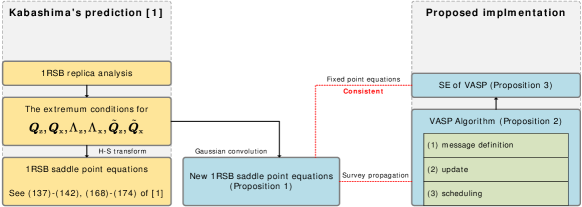
Figure 2: Structure of the main results

In this paper, we propose a new algorithm to fulfill Kabashima’s 1RSB prediction for the mismatched GLM problem with a rotation-variant measurement matrix. The algorithm, termed vector approximate survey propagation (VASP), is named after ASP [21] and GASP [23] but with a new emphasis on the vector form of the survey. Survey propagation [27, 29, 30, 31] is a message passing procedure similar to the classical loopy belief propagation [10] with crucial differences in message definition, update, scheduling and other aspects. Survey propagation was developed in statistical physics using the cavity method. Generally speaking, a survey is a weighted sum of believes propagating in the factor graph of the inference problem. In a complex disordered system, the global configuration space may separate into many distant clusters, and belief propagation may not hold globally, but it might converge if one restricts the probability space to a given cluster [29]. In this context, a survey considers all the clusters, attributes to each a probability proportional to the number of configurations, and sums them up after weighing with the probabilities.

Our derivation for a new algorithm starts from the reformulation of Kabashima’s 1RSB prediction. As outlined in Fig. 2, we utilize a Gaussian convolution formula to replace (a second use of) the Hubbard-Stratonovich transform and successfully decouple the replicated variables to finally arrive at a new set of saddle point equations that are mathematically equivalent to [1]. The so-called overlap quantity here can avoid the issue with the ground truth $\bm{x}_{0}$ that existed in the estimator’s input. A log-partition function that follows further links the underlying prior and likelihood to the form of a survey. Motivated by the new findings, we extend the survey into a vector form, design the associated updating rules, and schedule the propagation in an iterative manner. We obtain the VASP algorithm, and derive an SE for it, assuming empirical convergence on the related variables. We also verify the effectiveness of the new results by Monte Carlo simulations, and the simulation results are compared with the competing algorithms.

In summary, this paper contributes in two aspects: (i) We propose VASP, a survey propagation algorithm, for approximate inference in the large system limit under a mismatched generalized linear model with rotation-invariant measurement matrices. The computational complexity of VASP is as low as VAMP, which is on the order of $O(N^{3})$, with $N$ being the problem size. We empirically show, in situations where RSB typically occurs (e.g., the log-posterior is non-convex), VASP significantly outperforms the state-of-the-art algorithms of AMP [8, 9, 2], (G)VAMP [18, 28, 5], and GASP [23]. In cases without RS breaking (e.g., the log-posterior is convex), VASP is shown to perform equally good as VAMP, whose optimality under the RS ansatz had already been verified [1]. We also demonstrate VASP embraces VAMP as a special case, by fixing the so-called Parasi parameter at $1$ and approaching the weighting Gaussian’s variance towards $0$. (ii) We present an SE for VASP, which is shown to capture precisely the dynamical behaviors of the algorithm. We analyze the SE fixed point equations and surprisingly find that they perfectly agree with the saddle points of an optimal estimator, whose performance limits had been predicted by [1] under the 1RSB ansatz. The new finding suggests VASP converges to the optimal estimator in the large system limit, as long as the 1RSB ansatz is valid and the SE converges to the fixed point. In this context, VASP can be treated as an extension to VAMP for optimal approximate inference under the model-mismatch setting, as VASP is optimal even in the 1RSB case, which overcomes a fundamental limit of VAMP and fulfills the prediction of Kabashima’s.

Throughout this paper, we adopt the following notation conventions: non-bold lowercase letters (e.g., $m$ and $v$) represent scalars, bold lowercase letters (e.g., $\bm{m}$ and $\bm{v}$) denote column vectors, bold lowercase letters with a vector arrow (e.g., $\vec{\bm{m}}$ and $\vec{\bm{v}}$) indicate row vectors, and capital letters (e.g., $\bm{V}$ and $\bm{C}$) signify matrices. $\mathsf{e}(\cdot)$ represents an exponential operator. $\delta(\cdot)$ denotes a Dirac delta function. $\mathsf{N}[\bm{m},\bm{C}]$ denotes a Gaussian distribution with mean $\bm{m}$ and covariance $\bm{C}$, defined as $\mathsf{N}[\bm{x}|\bm{m},\bm{C}]\triangleq|2\pi\bm{C}|^{-1/2}\mathsf{e}[-1/2(\bm{x}-\bm{m})^{\mathsf{T}}\bm{C}^{-1}(\bm{x}-\bm{m})]$. For any matrix $\bm{A}$, $A^{(i,j)}$ represents the element at the $i$-th row and $j$-th column of $\bm{A}$. $\bm{A}^{\top}$ denotes the transpose of matrix $\bm{A}$. $\mathsf{Tr}(\bm{A})$ stands for the trace of matrix $\bm{A}$. $\bm{e}_{N}$ is a column vector of size $N$ filled with zeros, except for the first element which is set to $1$. $\bm{1}_{N}$ is a column vector of size $N$ consisting of all ones. $\bm{I}_{N}$ signifies the identity matrix of size $N$. $\mathbb{1}_{N}$ is a matrix of size $N$ containing all ones. $\mathsf{D}(\bm{v})$ is a diagonal matrix with diagonal elements equal to the elements of vector $\bm{v}$. $\mathsf{d}(\bm{C})$ is a diagonal operator, returning a $N$-dimensional column vector containing the diagonal elements of matrix $\bm{C}$. To keep the notations uncluttered this paper presents only the detail of the $\kappa=1$ case, while leaving the $\kappa\to+\infty$ case to the readers as it can be recovered easily by means of [32].

II Kabashima’s Prediction and A Reformulation

In this section, we revisit Kabashima’s results [24, 25, 33, 1, 26] on the 1RSB free energy of an optimal estimator in a model-mismatched GLM with rotation-invariant measurement matrix. We point out their result provides little information about the design of a concrete algorithm that may achieve the 1RSB prediction. For this reason, we re-derive the 1RSB saddle point equations by tracing back to the extreme conditions of Kabashima’s and applying a Gaussian convolution formula as the variable-decoupling trick. We then observe, from the reformulated equations, the approximating prior and likelihood functions take the form of a survey, which indicates an algorithm based on survey propagation may fulfill our target.

II-A Kabashima’s Replica Prediction for the Optimal Estimator

In [1], Takahashi and Kabashima evaluated the free energy of the estimator (3), which is optimal in the posterior sense under the model-mismatch setting, where the prior $q(\bm{x}_{0})$ and the likelihood $q(\bm{y}|\bm{z}_{0})$ are postulated and not necessarily equal the ground truth. By the replica method, the free energy was expressed as

$$f\triangleq -\lim_{\tau\rightarrow 0}\frac{1}{\tau}\mathop{\operatorname{extr}}\limits_{\bm{Q}_{\mathsf{z}},\bm{Q}_{\mathsf{x}}}[g_{\mathsf{z}}+g_{\mathsf{h}}-g_{\mathsf{d}}+g_{\mathsf{x}}],$$

$$g_{\mathsf{z}}\triangleq \mathop{\operatorname{extr}}\limits_{\tilde{\bm{Q}}_{\mathsf{z}}}[\frac{\alpha\mathsf{Tr}(\bm{Q}_{\mathsf{z}}\tilde{\bm{Q}}_{\mathsf{z}})}{2}+\alpha\log\int{\mathsf{d}y\mathsf{d}\vec{\bm{z}}}\,p(y\bm{1}|\vec{\bm{z}})\mathsf{e}(-\frac{\vec{\bm{z}}\tilde{\bm{Q}}_{\mathsf{z}}\vec{\bm{z}}^{\mathsf{T}}}{2})],$$

$$g_{\mathsf{h}}\triangleq \mathop{\operatorname{extr}}\limits_{\bm{\Lambda}_{\mathsf{z}},\bm{\Lambda}_{\mathsf{x}}}[\frac{\alpha\mathsf{Tr}(\bm{Q}_{\mathsf{z}}\bm{\Lambda}_{\mathsf{z}})}{2}-\frac{\mathbb{E}_{\lambda}[\log|\bm{\Lambda}_{\mathsf{x}}+\lambda\bm{\Lambda}_{\mathsf{z}}|]}{2}+\frac{\mathsf{Tr}(\bm{Q}_{\mathsf{x}}\bm{\Lambda}_{\mathsf{x}})}{2}],$$

$$g_{\mathsf{d}}\triangleq \frac{\alpha\log|\bm{Q}_{\mathsf{z}}|}{2}+\frac{\log|\bm{Q}_{\mathsf{x}}|}{2},$$

$$g_{\mathsf{x}}\triangleq \mathop{\operatorname{extr}}\limits_{\tilde{\bm{Q}}_{\mathsf{x}}}[\frac{\mathsf{Tr}(\bm{Q}_{\mathsf{x}}\tilde{\bm{Q}}_{\mathsf{x}})}{2}+\log\int{\mathsf{d}\vec{\bm{x}}}\,\mathsf{e}(-\frac{\vec{\bm{x}}\tilde{\bm{Q}}_{\mathsf{x}}\vec{\bm{x}}^{\mathsf{T}}}{2})p(\vec{\bm{x}})],$$

where $\mathop{\operatorname{extr}}(\cdot)$ is an extremum operator, $\bm{Q}_{\mathsf{z}}$, $\bm{Q}_{\mathsf{x}}$, $\bm{\Lambda}_{\mathsf{z}}$, $\bm{\Lambda}_{\mathsf{x}}$, $\tilde{\bm{Q}}_{\mathsf{z}}$, and $\tilde{\bm{Q}}_{\mathsf{x}}$ are $(\tau+1)\times(\tau+1)$ real symmetric matrices , $\lambda$ follows the limiting eigenvalue distribution of $\bm{H}^{\mathsf{T}}\bm{H}$, $\mathsf{d}\vec{\bm{z}}\triangleq\mathsf{d}z_{0}\mathsf{d}\tilde{z}_{1}\cdots\mathsf{d}\tilde{z}_{\tau}$ with $\vec{\bm{z}}\triangleq[z_{0},\tilde{z}_{1},\cdots,\tilde{z}_{\tau}]$, $\mathsf{d}\vec{\bm{x}}\triangleq\mathsf{d}x_{0}\mathsf{d}\tilde{x}_{1}\cdots\mathsf{d}\tilde{x}_{\tau}$ with $\vec{\bm{x}}\triangleq[x_{0},\tilde{x}_{1},\cdots,\tilde{x}_{\tau}]$, $p(y\bm{1}|\vec{\bm{z}})\triangleq p(y|z_{0})\prod_{i=1}^{\tau}q(y|\tilde{z}_{i})$, and $p(\vec{\bm{x}})\triangleq p(x_{0})\prod_{i=1}^{\tau}q(\tilde{x}_{i})$. The extremum conditions then read [1, eqs. (124)-(126)]:

$$\bm{0}= \bm{\Lambda}_{\mathsf{z}}-\bm{Q}_{\mathsf{z}}^{-1}+\tilde{\bm{Q}}_{\mathsf{z}},$$ (5a)

$$\bm{0}= \bm{\Lambda}_{\mathsf{x}}-\bm{Q}_{\mathsf{x}}^{-1}+\tilde{\bm{Q}}_{\mathsf{x}},$$ (5b)

$$\bm{Q}_{\mathsf{z}}= 1/\alpha\mathbb{E}_{\lambda}[\lambda(\bm{\Lambda}_{\mathsf{x}}+\lambda\bm{\Lambda}_{\mathsf{z}})^{-1}],$$ (5c)

$$\bm{Q}_{\mathsf{x}}= \mathbb{E}_{\lambda}[(\bm{\Lambda}_{\mathsf{x}}+\lambda\bm{\Lambda}_{\mathsf{z}})^{-1}],$$ (5d)

$$\bm{Q}_{\mathsf{z}}= \frac{\int{\mathsf{d}y\mathsf{d}\vec{\bm{z}}}\,p(y\bm{1}|\vec{\bm{z}})\mathsf{e}(-1/2\vec{\bm{z}}\tilde{\bm{Q}}_{\mathsf{z}}\vec{\bm{z}}^{\mathsf{T}})\vec{\bm{z}}^{\mathsf{T}}\vec{\bm{z}}}{\int{\mathsf{d}y\mathsf{d}\vec{\bm{z}}}\,p(y\bm{1}|\vec{\bm{z}})\mathsf{e}(-1/2\vec{\bm{z}}\tilde{\bm{Q}}_{\mathsf{z}}\vec{\bm{z}}^{\mathsf{T}})},$$ (5e)

$$\bm{Q}_{\mathsf{x}}= \frac{\int{\mathsf{d}\vec{\bm{x}}}\,\mathsf{e}(-1/2\vec{\bm{x}}\tilde{\bm{Q}}_{\mathsf{x}}\vec{\bm{x}}^{\mathsf{T}})p(\vec{\bm{x}})\vec{\bm{x}}^{\mathsf{T}}\vec{\bm{x}}}{\int{\mathsf{d}\vec{\bm{x}}}\,\mathsf{e}(-1/2\vec{\bm{x}}\tilde{\bm{Q}}_{\mathsf{x}}\vec{\bm{x}}^{\mathsf{T}})p(\vec{\bm{x}})}.$$ (5f)

Under the 1RSB ansatz, it was showed the above conditions were further specified as [1, eqs. (137)-(142), (168)-(174)], which reproduced exactly the RS result by letting $\Delta=0$. The 1RSB ansatz says: solutions to the replica extremum condition exhibit the following matrix structure [27, 1, 34]

$$\bm{Q}_{\mathsf{z}}= \mathcal{Q}_{\tau+1,L}(C_{\mathsf{z}},D_{\mathsf{z}},F_{\mathsf{z}},G_{\mathsf{z}},H_{\mathsf{z}}),$$

$$\bm{Q}_{\mathsf{x}}= \mathcal{Q}_{\tau+1,L}(C_{\mathsf{x}},D_{\mathsf{x}},F_{\mathsf{x}},G_{\mathsf{x}},H_{\mathsf{x}}),$$

$$\bm{\Lambda}_{\mathsf{z}}= \mathcal{Q}_{\tau+1,L}(\hat{C}_{\mathsf{2z}},\hat{D}_{\mathsf{2z}},\hat{F}_{\mathsf{2z}},\hat{G}_{\mathsf{2z}},\hat{H}_{\mathsf{2z}}),$$

$$\bm{\Lambda}_{\mathsf{x}}= \mathcal{Q}_{\tau+1,L}(\hat{C}_{\mathsf{2x}},\hat{D}_{\mathsf{2x}},\hat{F}_{\mathsf{2x}},\hat{G}_{\mathsf{2x}},\hat{H}_{\mathsf{2x}}),$$

$$\tilde{\bm{Q}}_{\mathsf{z}}= \mathcal{Q}_{\tau+1,L}(\hat{C}_{\mathsf{1z}},\hat{D}_{\mathsf{1z}},\hat{F}_{\mathsf{1z}},\hat{G}_{\mathsf{1z}},\hat{H}_{\mathsf{1z}}),$$

$$\tilde{\bm{Q}}_{\mathsf{x}}= \mathcal{Q}_{\tau+1,L}(\hat{C}_{\mathsf{1x}},\hat{D}_{\mathsf{1x}},\hat{F}_{\mathsf{1x}},\hat{G}_{\mathsf{1x}},\hat{H}_{\mathsf{1x}}),$$

where $\mathcal{Q}_{\tau+1,L}(C,D,F,G,H)\triangleq\left[\begin{array}[]{cc}C&D\vec{\bm{1}}_{\tau}\\ D\bm{1}_{\tau}&\mathcal{A}_{\tau,L}(F,G,H)\\ \end{array}\right]$ and $\mathcal{A}_{\tau,L}(F,G,H)\triangleq F\mathbb{1}_{\tau}+(G-F)\bm{I}_{\tau}+H\bm{I}_{\tau/L}\otimes\mathbb{1}_{L}$.

A limitation of the above result is: little information can be obtained from the saddle point equations about how to design a practical estimator. In particular, the parameter $D_{\mathsf{x}}$, also known as the overlap [27] between $x_{0}$ and $\bar{x}(x_{0},\xi)$, was expressed as [1, eq. (171)]

$$D_{\mathsf{x}}= \lim_{\tau\to 0}\mathbb{E}[x_{0}\tilde{x}]=\int{\mathsf{d}x_{0}\mathsf{d}\xi}\,p(x_{0},\xi)x_{0}\bar{x}(x_{0},\xi),$$ (6)

where $\bar{x}(x_{0},\xi)$ is a random variable depending explicitly on $x_{0}$ and the auxiliary $\xi$. In the replica literature, e.g., [35, 36], an overlap is usually expressed as $D_{\mathsf{x}}=\mathbb{E}[x_{0}\hat{x}]$, in which $\hat{x}$ represents the output of some practical estimator. However, here the quantity $\bar{x}(x_{0},\xi)$ can not be interpreted as an estimate $\hat{x}$, because no practical estimator can have the ground truth $x_{0}$ as its input. Therefore, to reformulate the overlap into the desired form $D_{\mathsf{x}}=\mathbb{E}[x_{0}\hat{x}]$, we revisit the extremum conditions (5) and rewrite $D_{\mathsf{x}}$ as Line 23 of Tab. I, i.e.,

$$D_{\mathsf{x}}=\int{\mathsf{d}\mu_{\mathsf{x}}\mathsf{d}x_{0}}\,a_{\mathsf{x}}x_{0}\frac{\int{\mathsf{d}\beta}\,\mathsf{N}[\beta|\mu_{\mathsf{x}},\Delta_{\mathsf{x1}}]\mathsf{e}[Lg_{\mathsf{x0}}]\langle\tilde{x}\rangle}{\mathsf{e}[g_{\mathsf{x1}}]}\triangleq\mathbb{E}[x_{0}\hat{x}(\mu_{\mathsf{x}})],$$

where $a_{\mathsf{x}}$ is the joint distribution of $x_{0}$ and $\mu_{\mathsf{x}}$, and $\hat{x}(\mu_{\mathsf{x}})$ is a deterministic function of $\mu_{\mathsf{x}}$, which is also independent of $x_{0}$. For $\hat{x}(\mu_{\mathsf{x}})$, we find out that its denominator, i.e., $\mathsf{e}[g_{\mathsf{x1}}]$, is the log-partition function of the desired posterior, which is directly connected to a survey as already defined in [23, 21].

II-B Reformulation of 1RSB Saddle Point Equations

In this paper, we just provide a brief description of the reformulation procedure, with detailed information available in Appendix A. We next take steps to reformulate the 1RSB saddle point equations, but we start from the extremum conditions (5). For conciseness, we put all notations into Tab. IV of the Appendix.

(S1) Under the 1RSB ansatz, (5a)-(5b) are specified as Lines 7-14 of Tab. I, together with

$$0= \hat{C}_{\mathsf{1z}}+\hat{C}_{\mathsf{2z}}-1/C_{\mathsf{z}},$$ (7)

$$0= \hat{C}_{\mathsf{1x}}+\hat{C}_{\mathsf{2x}}-1/C_{\mathsf{x}}.$$ (8)

(S2) Similarly, (5c)-(5d) produce Lines 17-18 and 21-22 of Tab. I, where

$$\theta\triangleq (\hat{G}_{\mathsf{2x}}-\hat{F}_{\mathsf{2x}}+L\hat{H}_{\mathsf{2x}})+\lambda(\hat{G}_{\mathsf{2z}}-\hat{F}_{\mathsf{2z}}+L\hat{H}_{\mathsf{2z}}),$$

$$\theta_{0}\triangleq (\hat{G}_{\mathsf{2x}}-\hat{F}_{\mathsf{2x}})+\lambda(\hat{G}_{\mathsf{2z}}-\hat{F}_{\mathsf{2z}}),$$

together with the followings:

$$C_{\mathsf{z}}= 1/\alpha\mathbb{E}_{\lambda}[\lambda/(\hat{C}_{\mathsf{2x}}+\lambda\hat{C}_{\mathsf{2z}})],$$ (9)

$$D_{\mathsf{z}}= -\frac{1}{\alpha}\mathbb{E}_{\lambda}[\frac{\lambda(\hat{D}_{\mathsf{2x}}+\lambda\hat{D}_{\mathsf{2z}})}{(\hat{C}_{\mathsf{2x}}+\lambda\hat{C}_{\mathsf{2z}})\theta}],$$ (10)

$$F_{\mathsf{z}}= \frac{1}{\alpha}\mathbb{E}_{\lambda}[\frac{\lambda(\hat{D}_{\mathsf{2x}}+\lambda\hat{D}_{\mathsf{2z}})^{2}}{(\hat{C}_{\mathsf{2x}}+\lambda\hat{C}_{\mathsf{2z}})\theta^{2}}]-\frac{1}{\alpha}\mathbb{E}_{\lambda}[\frac{\lambda(\hat{F}_{\mathsf{2x}}+\lambda\hat{F}_{\mathsf{2z}})}{\theta^{2}}],$$ (11)

$$C_{\mathsf{x}}= \mathbb{E}_{\lambda}[1/(\hat{C}_{\mathsf{2x}}+\lambda\hat{C}_{\mathsf{2z}})],$$ (12)

$$D_{\mathsf{x}}= -\mathbb{E}_{\lambda}[\frac{\hat{D}_{\mathsf{2x}}+\lambda\hat{D}_{\mathsf{2z}}}{(\hat{C}_{\mathsf{2x}}+\lambda\hat{C}_{\mathsf{2z}})\theta}],$$ (13)

$$F_{\mathsf{x}}= \mathbb{E}_{\lambda}[\frac{(\hat{D}_{\mathsf{2x}}+\lambda\hat{D}_{\mathsf{2z}})^{2}}{(\hat{C}_{\mathsf{2x}}+\lambda\hat{C}_{\mathsf{2z}})\theta^{2}}]-\mathbb{E}_{\lambda}[\frac{\hat{F}_{\mathsf{2x}}+\lambda\hat{F}_{\mathsf{2z}}}{\theta^{2}}].$$ (14)

(S3) The reformulation of (5f) starts from the expansion of $\mathsf{e}(-1/2\vec{\bm{x}}\tilde{\bm{Q}}_{x}\vec{\bm{x}}^{\mathsf{T}})$ detailed as below:

$$\mathsf{e}(-1/2\vec{\bm{x}}\tilde{\bm{Q}}_{x}\vec{\bm{x}}^{\mathsf{T}})\overset{\text{(a)}}{=} \mathsf{e}[-\frac{1}{2}(\hat{C}_{\mathsf{1x}}-\frac{\hat{D}_{\mathsf{1x}}^{2}}{\hat{F}_{\mathsf{1x}}})x_{0}^{2}]\underbrace{\mathsf{e}[-\frac{1}{2}(\frac{\hat{D}_{\mathsf{1x}}}{\sqrt{\hat{F}_{\mathsf{1x}}}}x_{0}+\sum_{i=1}^{\tau}\sqrt{\hat{F}_{\mathsf{1x}}}\tilde{x}_{i})^{2}]}_{E_{\mathsf{1}}}\times$$

$$\mathsf{e}[-\frac{1}{2}(\hat{G}_{\mathsf{1x}}-\hat{F}_{\mathsf{1x}})\sum_{i=1}^{\tau}\tilde{x}_{i}^{2}]\underbrace{\mathsf{e}[-\frac{1}{2}\hat{H}_{\mathsf{1x}}\sum_{i=1}^{\tau/L}(\sum_{j=1}^{L}\tilde{x}_{L(i-1)+j})^{2}]}_{E_{\mathsf{2}}},$$

where (a) follows from Lemma 1. The main technical challenge here lies in $E_{\mathsf{1}}$ and $E_{\mathsf{2}}$; each generates many cross terms, making the high-dimensional integral (5f) intractable. A classical solution is to use the Hubbard-Stratonovich transform , and in [1] they used its twice, one for each. By contrast, we only use the H-S transform once, and meanwhile use the convolution of Gaussian densities [40]. Our result is

$$\mathsf{e}(-1/2\vec{\bm{x}}\tilde{\bm{Q}}_{x}\vec{\bm{x}}^{\mathsf{T}})\overset{\text{(b)}}{\propto} \int{\mathsf{d}\mu_{\mathsf{x}}}\,\mathsf{e}(-\eta_{\mathsf{x}}\mu_{\mathsf{x}}^{2})\mathsf{e}[-\frac{1}{2}(\hat{C}_{\mathsf{1x}}-\frac{\hat{D}_{\mathsf{1x}}^{2}}{\hat{F}_{\mathsf{1x}}})x_{0}^{2}+\frac{\mathbb{j}\sqrt{2\eta_{\mathsf{x}}}\hat{D}_{\mathsf{1x}}}{\sqrt{\hat{F}_{\mathsf{1x}}}}x_{0}\mu_{\mathsf{x}}]\times$$

$$\prod_{i=1}^{\tau/L}\mathsf{e}[\mathbb{j}\sqrt{2\eta_{\mathsf{x}}\hat{F}_{\mathsf{1x}}}\mu_{\mathsf{x}}(\sum_{j=1}^{L}\tilde{x}_{L(i-1)+j})-\frac{1}{2}(\hat{G}_{\mathsf{1x}}-\hat{F}_{\mathsf{1x}}+\hat{H}_{\mathsf{1x}})\times$$

$$(\sum_{j=1}^{L}\tilde{x}_{L(i-1)+j}^{2})-\frac{1}{2}\hat{H}_{\mathsf{1x}}\sum_{j\neq k}^{L}\tilde{x}_{L(i-1)+j}\tilde{x}_{L(i-1)+k}]$$

$$\overset{\text{(c)}}{\propto} \int{\mathsf{d}\mu_{\mathsf{x}}}\,\mathsf{e}(-\eta_{\mathsf{x}}\mu_{\mathsf{x}}^{2})\mathsf{e}[-\frac{1}{2}(\hat{C}_{\mathsf{1x}}-\frac{\hat{D}_{\mathsf{1x}}^{2}}{\hat{F}_{\mathsf{1x}}})x_{0}^{2}+\frac{\mathbb{j}\sqrt{2\eta_{\mathsf{x}}}\hat{D}_{\mathsf{1x}}}{\sqrt{\hat{F}_{\mathsf{1x}}}}x_{0}\mu_{\mathsf{x}}]\times$$

$$\prod_{i=1}^{\tau/L}\int{\mathsf{d}\beta}\,\mathsf{N}[\beta|m_{\mathsf{x}},\Delta_{\mathsf{x1}}]\prod_{j=1}^{L}{}\mathsf{N}[\tilde{x}_{L(i-1)+j}|\beta,\Delta_{\mathsf{x0}}],$$

where (b) uses the H-S transform and (c) uses the Gaussian density convolution [40], and $m_{\mathsf{x}}$, $\Delta_{\mathsf{x0}}$, $\Delta_{\mathsf{x1}}$ are defined as Lines 1-3 of Tab. IV. The denominator of (5f) is given as:

$$\int{\mathsf{d}\vec{\bm{x}}}\,\mathsf{e}(-\frac{\vec{\bm{x}}\tilde{\bm{Q}}_{\mathsf{x}}\vec{\bm{x}}^{\mathsf{T}}}{2})p(\vec{\bm{x}})\propto\int{\mathsf{d}\mu_{\mathsf{x}}}\,\mathsf{e}(-\eta_{\mathsf{x}}\mu_{\mathsf{x}}^{2})\mathsf{e}(\frac{\tau}{L}g_{\mathsf{x1}})\int{\mathsf{d}x_{0}}\,b_{\mathsf{x}}p(x_{0}),$$

with $b_{\mathsf{x}}$, $\langle a\rangle$, $g_{\mathsf{x0}}$, $g_{\mathsf{x1}}$ defined as lines 4-7 of Tab. IV. So far, the extremum condition in (5f) yields the following equations:

$$C_{\mathsf{x}}=\frac{1}{\mathsf{C}_{\mathsf{x}}}\int{\mathsf{d}\mu_{\mathsf{x}}\mathsf{d}x_{0}}h_{\mathsf{x}}x_{0}^{2},$$ (15)

$$D_{\mathsf{x}}=\frac{1}{\mathsf{C}_{\mathsf{x}}}\int{\mathsf{d}\mu_{\mathsf{x}}\mathsf{d}x_{0}}h_{\mathsf{x}}x_{0}\frac{\int{\mathsf{d}\beta}\mathsf{N}[\beta|m_{\mathsf{x}},\Delta_{\mathsf{x1}}]\mathsf{e}(Lg_{\mathsf{x0}})\langle\tilde{x}\rangle}{\mathsf{e}(g_{\mathsf{x1}})},$$ (16)

$$F_{\mathsf{x}}=\frac{1}{\mathsf{C}_{\mathsf{x}}}\int{\mathsf{d}\mu_{\mathsf{x}}\mathsf{d}x_{0}}h_{\mathsf{x}}[\frac{\int{\mathsf{d}\beta}\mathsf{N}[\beta|m_{\mathsf{x}},\Delta_{\mathsf{x1}}]\mathsf{e}(Lg_{\mathsf{x0}})\langle\tilde{x}\rangle}{\mathsf{e}(g_{\mathsf{x1}})}]^{2},$$ (17)

$$G_{\mathsf{x}}+H_{\mathsf{x}}=\frac{1}{\mathsf{C}_{\mathsf{x}}}\int{\mathsf{d}\mu_{\mathsf{x}}\mathsf{d}x_{0}}h_{\mathsf{x}}\frac{\int{\mathsf{d}\beta}\mathsf{N}[\beta|m_{\mathsf{x}},\Delta_{\mathsf{x1}}]\mathsf{e}(Lg_{\mathsf{x0}})\langle\tilde{x}^{2}\rangle}{\mathsf{e}(g_{\mathsf{x1}})},$$ (18)

$$F_{\mathsf{x}}+H_{\mathsf{x}}=\frac{1}{\mathsf{C}_{\mathsf{x}}}\int{\mathsf{d}\mu_{\mathsf{x}}\mathsf{d}x_{0}}h_{\mathsf{x}}\frac{\int{\mathsf{d}\beta}\mathsf{N}[\beta|m_{\mathsf{x}},\Delta_{\mathsf{x1}}]\mathsf{e}(Lg_{\mathsf{x0}})\langle\tilde{x}\rangle^{2}}{\mathsf{e}(g_{\mathsf{x1}})},$$ (19)

with

$$h_{\mathsf{x}}\triangleq \mathsf{N}[\mu_{\mathsf{x}}|\frac{\mathbb{j}\hat{D}_{\mathsf{1x}}}{\sqrt{2\eta_{\mathsf{x}}\hat{F}_{\mathsf{1x}}}}x_{0},\frac{1}{2\eta_{\mathsf{x}}}]\mathsf{e}(-1/2\hat{C}_{\mathsf{1x}}x_{0}^{2})p(x_{0}),$$

$$\mathsf{C}_{\mathsf{x}}\triangleq \int{\mathsf{d}\mu_{\mathsf{x}}\mathsf{d}x_{0}}\,h_{\mathsf{x}}=\int{\mathsf{d}x_{0}}\,\mathsf{e}(-1/2\hat{C}_{\mathsf{1x}}x_{0}^{2})p(x_{0}).$$

(S4) The reformulation for (5e) is similar, which includes $C_{\mathsf{z}}$ in Line 5 of Tab. I and the following equations:

$$D_{\mathsf{z}}=\int{\mathsf{d}y\mathsf{d}z_{0}\mathsf{d}\mu_{\mathsf{z}}}h_{\mathsf{z}}z_{0}\frac{\int{\mathsf{d}\beta}\mathsf{N}[\beta|m_{\mathsf{z}},\Delta_{\mathsf{z1}}]\mathsf{e}[Lg_{\mathsf{z0}}]\langle\tilde{z}\rangle}{\mathsf{e}[g_{\mathsf{z1}}]},$$ (20)

$$F_{\mathsf{z}}=\int{\mathsf{d}y\mathsf{d}z_{0}\mathsf{d}\mu_{\mathsf{z}}}h_{\mathsf{z}}[\frac{\int{\mathsf{d}\beta}\mathsf{N}[\beta|m_{\mathsf{z}},\Delta_{\mathsf{z1}}]\mathsf{e}[Lg_{\mathsf{z0}}]\langle\tilde{z}\rangle}{\mathsf{e}[g_{\mathsf{z1}}]}]^{2},$$ (21)

$$G_{\mathsf{z}}+H_{\mathsf{z}}=\int{\mathsf{d}y\mathsf{d}z_{0}\mathsf{d}\mu_{\mathsf{z}}}h_{\mathsf{z}}\frac{\int{\mathsf{d}\beta}\mathsf{N}[\beta|m_{\mathsf{z}},\Delta_{\mathsf{z1}}]\mathsf{e}[Lg_{\mathsf{z0}}]\langle\tilde{z}^{2}\rangle}{\mathsf{e}[g_{\mathsf{z1}}]},$$ (22)

$$F_{\mathsf{z}}+H_{\mathsf{z}}=\int{\mathsf{d}y\mathsf{d}z_{0}\mathsf{d}\mu_{\mathsf{z}}}h_{\mathsf{z}}\frac{\int{\mathsf{d}\beta}\mathsf{N}[\beta|m_{\mathsf{z}},\Delta_{\mathsf{z1}}]\mathsf{e}[Lg_{\mathsf{z0}}]\langle\tilde{z}\rangle^{2}}{\mathsf{e}[g_{\mathsf{z1}}]},$$ (23)

with $m_{\mathsf{z}}$, $\Delta_{\mathsf{z0}}$, $\Delta_{\mathsf{z1}}$, $b_{\mathsf{z}}$, $\langle a\rangle$, $g_{\mathsf{z0}}$, and $g_{\mathsf{z1}}$ defined as Lines 1-7 of Tab. IV and

$$h_{\mathsf{z}}\triangleq p(y|z_{0})\mathsf{N}[z_{0}|\frac{\mathbb{j}\hat{D}_{\mathsf{1z}}\sqrt{\frac{2\eta_{\mathsf{z}}}{\hat{F}_{\mathsf{1z}}}}}{\hat{C}_{\mathsf{1z}}-\frac{\hat{D}_{\mathsf{1z}}^{2}}{\hat{F}_{\mathsf{1z}}}}\mu_{\mathsf{z}},\frac{1}{\hat{C}_{\mathsf{1z}}-\frac{\hat{D}_{\mathsf{1z}}^{2}}{\hat{F}_{\mathsf{1z}}}}]\mathsf{N}[\mu_{\mathsf{z}}|0,\frac{\hat{C}_{\mathsf{1z}}-\frac{\hat{D}_{\mathsf{1z}}^{2}}{\hat{F}_{\mathsf{1z}}}}{2\eta_{\mathsf{z}}\hat{C}_{\mathsf{1z}}}].$$

(S5) So far, we have obtained Lines 5, 7-14, 17-18, and 21-22 of Tab. I. To arrive at the remaining lines, we further take the following steps on the basis of (7)-(23):

• Substitute Line 5 of Tab. I into (7) and obtain Line 6;

• Combine Line 6 into (12) and obtain Line 3;

• Substitute Lines 3 and 6 into (8)-(11) and (13)-(15) and obtain Lines 1-2, 4, 15-16 and 19-20;

• Set $\eta_{\mathsf{z}}$ and $\eta_{\mathsf{x}}$ in accordance with Line 8 of Tab. IV, provided that the two auxiliary parameters can be any positive numbers, and then rewrite (16)-(23) into Lines 23-30 of Tab. I.

Proposition 1 (1RSB saddle point equations).

The 1RSB saddle point equations in [1, eqs. (137)-(142), (168)-(174)] are mathematically equivalent to Tab. I obtained from a reformulation of the extremum conditions (5a)-(5f).

TABLE I: The 1RSB Saddle Point Equations

Now we show how our result in Tab. IV can be connected with survey propagation. Take the $\mathsf{x}$-related parameters as an example, we merge Line 6 into Line 7 of Tab. IV and obtain a log-partition function as follows:

$$g_{\mathsf{x1}}=\log\underbrace{\int{\mathsf{d}\beta}\,\mathsf{N}[\beta|m_{\mathsf{x}},\Delta_{\mathsf{x1}}][\int{\mathsf{d}\tilde{x}}\,\mathsf{N}[\tilde{x}|\beta,\Delta_{\mathsf{x0}}]q(\tilde{x})]^{L}}_{g},$$

where $g$ is the partition function of a random $\vec{\bm{x}}$ with posterior

$$\text{posterior}(\vec{\bm{x}})=\frac{1}{g}\underbrace{\prod_{l=1}^{L}q(\tilde{x}_{l})}_{\text{prior}}\underbrace{\int{\mathsf{d}\beta}\,\mathsf{N}[\beta|m_{\mathsf{x}},\Delta_{\mathsf{x1}}]\prod_{l=1}^{L}\mathsf{N}[\tilde{x}_{l}|\beta,\Delta_{\mathsf{x0}}]}_{\text{likelihood}}.$$

We emphasize here the above likelihood for $\vec{\bm{x}}$ is exactly in the same form as a survey defined by [23, 21] (the situation for $\vec{\bm{z}}$ is similar, while there the prior is a survey). Therefore, our reformulated results suggest an algorithm based on survey propagation may achieve Kabashima’s 1RSB prediction.

III The VASP Algorithm

In this section, we propose the vector approximate survey propagation (VASP) algorithm, whose basic building block is survey propagation. Survey propagation [27, 29, 30, 31] is a message passing procedure similar to the classical iterative algorithm of belief propagation [10], but with some crucial differences, e.g., message definition, update, and scheduling. It was developed in statistical physics using the cavity method. Qualitatively, a survey, expressed as $\tilde{p}_{a\to b}=\sum_{\kappa}p_{\kappa}\mathcal{M}_{a\to b}^{(\kappa)}$, is a weighted sum of believes sent from node $a$ to node $b$ in the factor graph underlying the inference problem. The parameter $\kappa$ is the cluster index, as the global configuration space of the problem may separate into many distant clusters. Although the belief propagation does not hold globally, it would hold if one could restrict the probability space to a given cluster [29]. Within that restricted space, belief propagation would converge to a set of messages which depends on the cluster. For that reason, the cavity method uses a statistical approach to consider all the clusters, attribute to each cluster a probability $p_{\kappa}$ proportional to the number of configurations that it contains, weighs each belief $\mathcal{M}_{a\to b}^{(\kappa)}$ with a cluster-specific probability, and sum up the weighted believes over different clusters.

III-A Definition of Vector Survey

We define a replicated matrix for the target vector $\bm{x}$ for problem (2): $\bm{X}\triangleq[\bm{x}_{1},\cdots,\bm{x}_{L}]\triangleq[\vec{\bm{x}}_{1}^{\mathsf{T}},\cdots,\vec{\bm{x}}_{N}^{\mathsf{T}}]^{\mathsf{T}}\in\mathbb{R}^{N\times L}$, and subsequently define $\bm{Z}\triangleq\bm{H}\bm{X}\triangleq[\bm{z}_{1},\cdots,\bm{z}_{L}]\triangleq[\vec{\bm{z}}_{1}^{\mathsf{T}},\cdots,\vec{\bm{z}}_{M}^{\mathsf{T}}]^{\mathsf{T}}\in\mathbb{R}^{M\times L}$. We define the vector survey for $\bm{X}$:

$$\tilde{p}(\bm{X})\triangleq \prod_{i=1}^{N}\int{\mathsf{d}\beta}\,\mathsf{N}[\beta|\mu_{i},v_{1,i}]\prod_{l=1}^{L}\mathsf{N}[\tilde{x}_{l}|\beta,v_{0,i}]$$ (24)

$$= \prod_{i=1}^{N}\mathsf{N}[\vec{\bm{x}}_{i}|\mu_{i}\vec{\bm{1}}_{L},v_{1,i}\mathbb{1}_{L}+v_{0,i}\bm{I}_{L}].$$ (25)

The form of this definition elucidates why we are considering a replicated system [21]: if the posterior measure (4) develops a 1RSB structure, the phase space of the solutions of the inference problem gets clustered in exponentially many basins of solutions [27]. Therefore, if we consider a set of $L$ replicas of the same inference problem and we infinitesimally couple them, they will acquire a finite probability to fall inside the same cluster of solutions. The replicated system in GASP [23] was for scalar-site replicas; however, vector-site replicated variables are involved here, and we define the vector survey.

For manipulation convenience, we also vectorize the above matrices: $\tilde{\bm{x}}\triangleq\text{vec}(\bm{X})$, $\tilde{\bm{z}}\triangleq\text{vec}(\bm{Z})$, and $\tilde{\bm{H}}\triangleq\bm{I}_{L}\otimes\bm{H}$, with $\otimes$ being a Hadamard product. In this context, the survey of $\bm{X}$ can be re-denoted as $\tilde{p}(\tilde{\bm{x}})$, i.e.,

$$\tilde{p}(\tilde{\bm{x}})=\mathsf{N}[\tilde{\bm{x}}|\bm{1}_{L}\otimes\bm{\mu},\bm{\Delta}(\bm{v}_{0},\bm{v}_{1})]=\eqref{Eq:Def_VS:Gau_Form},$$

where $\bm{\mu}\triangleq[\mu_{1},\cdots,\mu_{N}]^{\mathsf{T}}$, $\bm{v}_{0}\triangleq[v_{0,1},\cdots,v_{0,N}]^{\mathsf{T}}$, $\bm{v}_{1}\triangleq[v_{1,1},\cdots,v_{1,N}]^{\mathsf{T}}\in\mathbb{R}^{N\times 1}$, and $\bm{\Delta}(\bm{v}_{0},\bm{v}_{1})\triangleq\mathbb{1}_{L}\otimes\mathsf{D}(\bm{v}_{1})+\bm{I}_{L}\otimes\mathsf{D}(\bm{v}_{0})\in\mathbb{R}^{NL\times NL}$. Also, it holds : $\bm{\Delta}^{-1}(\bm{v}_{0},\bm{v}_{1})=\mathbb{1}_{L}\otimes\mathsf{D}[(\bm{1}/\bm{v}-\bm{1}/\bm{v}_{0})/L]+\bm{I}_{L}\otimes\mathsf{D}(\bm{1}/\bm{v}_{0})$ with $\bm{v}\triangleq\bm{v}_{0}+L\bm{v}_{1}$.

III-B Update for Vector Survey

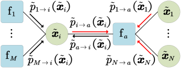
Figure 3: Generic factor graph for explaining the survey update

To illustrate our updating rules for the vector survey, we need the aid of a generic factor graph given as Fig. 3. In the factor graph, we assume all surveys to be initialized as multivariate Gaussian. We update the survey propagated from a variable node (VN) $\tilde{\bm{x}}_{i}$ to a factor node (FN) $\mathsf{f}_{a}$ in this way

$$\tilde{p}_{i\rightarrow a}(\tilde{\bm{x}}_{i})\propto\prod_{b\neq a}^{M}{}\tilde{p}_{b\rightarrow i}(\tilde{\bm{x}}_{i})=\mathsf{N}[\tilde{\bm{x}}_{i}|\bm{1}_{L}\otimes\bm{m}_{i\rightarrow a},\bm{\Delta}(\bm{v}_{i\rightarrow a,0},\bm{v}_{i\rightarrow a,1})],$$

where $\tilde{p}_{i\rightarrow a}(\tilde{\bm{x}}_{i})$ is still Gaussian, thanks to a property called Gaussian reproducing . Similarly, the survey from the FN $\mathsf{f}_{a}$ to the VN $\tilde{\bm{x}}_{i}$ is updated as

$$\tilde{p}_{a\rightarrow i}(\tilde{\bm{x}}_{i})\propto \mathsf{Proj}[\tilde{\mathsf{f}}_{a\rightarrow i}(\tilde{\bm{x}}_{i})\tilde{p}_{i\rightarrow a}(\tilde{\bm{x}}_{i})]/\tilde{p}_{i\rightarrow a}(\tilde{\bm{x}}_{i}),$$ (26)

where $\tilde{\mathsf{f}}_{a\rightarrow i}(\tilde{\bm{x}}_{i})\triangleq\int{\mathsf{d}\tilde{\bm{x}}_{j}}\mathsf{f}_{a}(\tilde{\bm{x}}_{1},\cdots,\tilde{\bm{x}}_{N})\prod_{j\neq i}^{N}{}\tilde{p}_{j\rightarrow a}(\tilde{\bm{x}}_{j})$, and the projection $\mathsf{Proj}[g(\tilde{\bm{x}})]$ approximates a generic function $g(\tilde{\bm{x}})$ as a multivariate Gaussian, by minimizing the Kullback-Leibler divergence (KLD) among all possible Gaussians, i.e.,

$$\mathsf{Proj}[g(\tilde{\bm{x}})]\triangleq\mathop{\operatorname{argmin}}\limits_{h\in\mathrm{Gaussian}}\mathrm{KL}[g\|h]=\mathsf{N}[\tilde{\bm{x}}|\bm{1}_{L}\otimes\bm{m}_{g},\bm{\Delta}(\bm{v}_{g,0},\bm{v}_{g,1})],$$

where $\mathrm{KL}[g\|h]\triangleq\int{\mathsf{d}\tilde{\bm{x}}}\,g(\tilde{\bm{x}})\log{g(\tilde{\bm{x}})}/{h(\tilde{\bm{x}})}$, and the minimization here reduces to the so-called moment matching [42]

$$\bm{1}_{L}\otimes\bm{m}_{g}= \frac{\int{\mathsf{d}\tilde{\bm{x}}}\,g(\tilde{\bm{x}})\tilde{\bm{x}}}{\int{\mathsf{d}\tilde{\bm{x}}}\,g(\tilde{\bm{x}})},$$

$$\bm{\Delta}(\bm{v}_{g,0},\bm{v}_{g,1})= \mathbb{d}[\frac{\int{\mathsf{d}\tilde{\bm{x}}}\,g(\tilde{\bm{x}})(\tilde{\bm{x}}-\bm{1}_{L}\otimes\bm{m}_{g})(\tilde{\bm{x}}-\bm{1}_{L}\otimes\bm{m}_{g})^{\mathsf{T}}}{\int{\mathsf{d}\tilde{\bm{x}}}\,g(\tilde{\bm{x}})}],$$

with $\mathbb{d}(\bm{A})\triangleq[\mathsf{d}(\bm{A}^{(i,j)})]$, $\bm{A}\triangleq[\bm{A}^{(i,j)}]\in\mathbb{R}^{MN\times MN}$, and $\bm{A}^{(i,j)}\in\mathbb{R}^{N\times N}$. For (26), we evaluate the numerator as $\mathsf{N}[\tilde{\bm{x}}_{i}|\bm{1}_{L}\otimes\hat{\bm{m}}_{i\rightarrow a},\bm{\Delta}(\hat{\bm{v}}_{a\rightarrow i,0},\hat{\bm{v}}_{a\rightarrow i,1})]$. Then, we calculate the entire fraction by using the Gaussian reproducing, i.e.,

$$\eqref{Fig:Survey}= \mathsf{N}[\tilde{\bm{x}}_{i}|\bm{1}_{L}\otimes\tilde{\bm{m}}_{a\rightarrow i},\bm{\Delta}(\tilde{\bm{v}}_{a\rightarrow i,0},\tilde{\bm{v}}_{a\rightarrow i,1})],$$

$$\bm{\Delta}(\tilde{\bm{v}}_{a\rightarrow i,0},\tilde{\bm{v}}_{a\rightarrow i,1})= [\bm{\Delta}^{-1}(\hat{\bm{v}}_{a\rightarrow i,0},\hat{\bm{v}}_{a\rightarrow i,1})-\bm{\Delta}^{-1}(\bm{v}_{i\rightarrow a,0},\bm{v}_{i\rightarrow a,1})]^{-1},$$

$$\bm{1}_{L}\otimes\tilde{\bm{m}}_{a\rightarrow i}= \bm{\Delta}(\tilde{\bm{v}}_{a\rightarrow i,0},\tilde{\bm{v}}_{a\rightarrow i,1})[\bm{\Delta}^{-1}(\hat{\bm{v}}_{a\rightarrow i,0},\hat{\bm{v}}_{a\rightarrow i,1})(\bm{1}_{L}\otimes\hat{\bm{m}}_{a\rightarrow i}-$$

$$\bm{\Delta}^{-1}(\bm{v}_{i\rightarrow a,0},\bm{v}_{i\rightarrow a,1})(\bm{1}_{L}\otimes\bm{m}_{i\rightarrow a}].$$

III-C Schedule of Vector Survey Propagation

Figure 4: Replicated factor graph for the inference problem

In this part, we provide a brief derivation of the VASP algorithm, with detailed information available in Appendix B. Prior to propagation scheduling, we provide first a replicated factor graph that corresponds to the inference problem. The factor graph is given as Fig. 4, where $p_{\mathsf{x}}^{+,t}(\tilde{\bm{x}})$ is the survey from $q(\tilde{\bm{x}})$ to $\tilde{\bm{x}}$, $p_{\mathsf{x}}^{-,t}(\tilde{\bm{x}})$ is from $\delta(\tilde{\bm{z}}-\tilde{\bm{H}}\tilde{\bm{x}})$ to $\tilde{\bm{x}}$, $p_{\mathsf{z}}^{+,t}(\tilde{\bm{z}})$ is from $\delta(\tilde{\bm{z}}-\tilde{\bm{H}}\tilde{\bm{x}})$ to $\tilde{\bm{z}}$, and $p_{\mathsf{z}}^{-,t}(\tilde{\bm{z}})$ from $q(\bm{y}|\tilde{\bm{z}})$ to $\tilde{\bm{z}}$. We now schedule the propagation in the following manner:

• Backward propagation (right to left in Fig. 4):

  $$p_{\mathsf{z}}^{-,t}(\tilde{\bm{z}})\propto \mathsf{Proj}[q(\bm{y}|\tilde{\bm{z}})p_{\mathsf{z}}^{+,t}(\tilde{\bm{z}})]/p_{\mathsf{z}}^{+,t}(\tilde{\bm{z}}),$$ (27)

  $$p_{\mathsf{x}}^{-,t}(\tilde{\bm{x}})\propto \mathsf{Proj}[f_{\mathsf{x}}^{-,t}(\tilde{\bm{x}})p_{\mathsf{x}}^{+,t}(\tilde{\bm{x}})]/p_{\mathsf{x}}^{+,t}(\tilde{\bm{x}}),$$ (28)

  $$f_{\mathsf{x}}^{-,t}(\tilde{\bm{x}})\triangleq \int{\mathsf{d}\tilde{\bm{z}}}\,\delta(\tilde{\bm{z}}-\tilde{\bm{H}}\tilde{\bm{x}})p_{\mathsf{z}}^{-,t}(\tilde{\bm{z}}).$$ (29)

• Forward propagation (left to right in Fig. 4):

  $$p_{\mathsf{x}}^{+,t+1}(\tilde{\bm{x}})\propto \mathsf{Proj}[q(\tilde{\bm{x}})p_{\mathsf{x}}^{-,t}(\tilde{\bm{x}})]/p_{\mathsf{x}}^{-,t}(\tilde{\bm{x}}),$$ (30)

  $$p_{\mathsf{z}}^{+,t+1}(\tilde{\bm{z}})\propto \mathsf{Proj}[f_{\mathsf{z}}^{+,t+1}(\tilde{\bm{z}})p_{\mathsf{z}}^{-,t}(\tilde{\bm{z}})]/p_{\mathsf{z}}^{-,t}(\tilde{\bm{z}}),$$ (31)

  $$f_{\mathsf{z}}^{+,t+1}(\tilde{\bm{z}})\triangleq \int{\mathsf{d}\tilde{\bm{x}}}\,\delta(\tilde{\bm{z}}-\tilde{\bm{H}}\tilde{\bm{x}})p_{\mathsf{x}}^{+,t+1}(\tilde{\bm{x}}).$$ (32)

• Go back to the backward propagation and iterate until the stopping condition is met.

Before the iteration, we initialize all forward surveys as

$$p_{\mathsf{z}}^{+,t}(\tilde{\bm{z}})\triangleq \mathsf{N}[\tilde{\bm{z}}|\bm{1}_{L}\otimes\bm{\mu}_{\mathsf{z}}^{+,t},\bm{\Delta}(\bm{v}_{\mathsf{z},0}^{+,t},\bm{v}_{\mathsf{z},1}^{+,t})],$$

$$p_{\mathsf{x}}^{+,t}(\tilde{\bm{x}})\triangleq \mathsf{N}[\tilde{\bm{x}}|\bm{1}_{L}\otimes\bm{\mu}_{\mathsf{x}}^{+,t},\bm{\Delta}(\bm{v}_{\mathsf{x},0}^{+,t},\bm{v}_{\mathsf{x},1}^{+,t})],$$

with $\bm{v}_{\mathsf{z}}^{+,t}\triangleq\bm{v}_{\mathsf{z},0}^{+,t}+L\bm{v}_{\mathsf{z},1}^{+,t}$ and $\bm{v}_{\mathsf{x}}^{+,t}\triangleq\bm{v}_{\mathsf{x},0}^{+,t}+L\bm{v}_{\mathsf{x},1}^{+,t}$.

For (27), we evaluate the formula, starting from its numerator, which can be rewritten as $\mathsf{N}[\tilde{\bm{z}}|\bm{1}_{L}\otimes\hat{\bm{\mu}}_{\mathsf{z}}^{-,t},\bm{\Delta}(\hat{\bm{v}}_{\mathsf{z},0}^{+,t},\hat{\bm{v}}_{\mathsf{z},1}^{+,t})]$, with $\hat{\bm{\mu}}_{\mathsf{z}}^{-,t}\triangleq[\hat{\mu}_{\mathsf{z},1}^{-,t},\cdots,\hat{\mu}_{\mathsf{z},M}^{-,t}]^{\mathsf{T}}$, $\hat{\bm{v}}_{\mathsf{z},0}^{-,t}\triangleq[\hat{v}_{\mathsf{z},0,1}^{-,t},\cdots,\hat{v}_{\mathsf{z},0,M}^{-,t}]^{\mathsf{T}}$, and $\hat{\bm{v}}_{\mathsf{z},1}^{-,t}\triangleq[\hat{v}_{\mathsf{z},1,1}^{-,t},\cdots,\hat{v}_{\mathsf{z},1,M}^{-,t}]^{\mathsf{T}}$. The parameters $\hat{\mu}_{\mathsf{z},a}^{-,t}$, $\hat{v}_{\mathsf{z},0,a}^{-,t}$ and $\hat{v}_{\mathsf{z},1,a}^{-,t}$ are defined as:

$$\hat{\mu}_{\mathsf{z},a}^{-,t}\triangleq \frac{\int{\mathsf{d}\beta}\,\mathsf{N}[\beta|\mu_{\mathsf{z},a}^{+,t},v_{\mathsf{z},1,a}^{+,t}]\mathsf{e}[Lg_{\mathsf{z0}}]\langle z\rangle}{\mathsf{e}[g_{\mathsf{z1}}]},$$

$$\hat{v}_{\mathsf{z},1,a}^{-,t}\triangleq \frac{\int{\mathsf{d}\beta}\,\mathsf{N}[\beta|\mu_{\mathsf{z},a}^{+,t},v_{\mathsf{z},1,a}^{+,t}]\mathsf{e}[Lg_{\mathsf{z0}}]\langle z\rangle^{2}}{\mathsf{e}[g_{\mathsf{z1}}]}-(\hat{\mu}_{\mathsf{z},a}^{-,t})^{2},$$

$$\hat{v}_{\mathsf{z},0,a}^{-,t}\triangleq \frac{\int{\mathsf{d}\beta}\,\mathsf{N}[\beta|\mu_{\mathsf{z},a}^{+,t},v_{\mathsf{z},1,a}^{+,t}]\mathsf{e}[Lg_{\mathsf{z0}}]\langle z^{2}\rangle}{\mathsf{e}[g_{\mathsf{z1}}]}-\hat{v}_{\mathsf{z},1,a}^{-,t}-(\hat{\mu}_{\mathsf{z},a}^{-,t})^{2},$$

where $\langle a\rangle$, $g_{\mathsf{z0}}$, and $g_{\mathsf{z1}}$ are given in Lines 10-12 of Tab. IV. Based on the numerator, we obtain the entire fraction by using the Gaussian reproduction property, where

$$\eqref{Eq:VSP:P_sz} =\mathsf{N}[\tilde{\bm{z}}|\bm{1}_{L}\otimes\bm{\mu}_{\mathsf{z}}^{-,t},\bm{\Delta}(\bm{v}_{\mathsf{z},0}^{-,t},\bm{v}_{\mathsf{z},1}^{-,t})],$$

with $\bm{v}_{\mathsf{z},1}^{-,t}\triangleq(\bm{v}_{\mathsf{z}}^{-,t}-\bm{v}_{\mathsf{z},0}^{-,t})/L$, $\bm{v}_{\mathsf{z},0}^{-,t}$, $\bm{v}_{\mathsf{z}}^{-,t}$, and $\bm{\mu}_{\mathsf{z}}^{-,t}$ given in Lines 7-9 of Tab. II.

For (28), we evaluate the projected term in the numerator:

$$f_{\mathsf{x}}^{-,t}(\tilde{\bm{x}})p_{\mathsf{x}}^{+,t}(\tilde{\bm{x}})= \mathsf{N}[\tilde{\bm{x}}|\bm{1}_{L}\otimes\hat{\bm{\mu}}_{\mathsf{x}}^{-,t},\hat{\bm{V}}_{\mathsf{x}}^{-,t}],$$

$$\hat{\bm{V}}_{\mathsf{x}}^{-,t}= \mathbb{1}_{L}\otimes[(\hat{\bm{C}}_{\mathsf{x}}^{-,t}-\hat{\bm{C}}_{\mathsf{x},0}^{-,t})/L]+\bm{I}_{L}\otimes\hat{\bm{C}}_{\mathsf{x},0}^{-,t},$$

$$\bm{1}_{L}\otimes\hat{\bm{\mu}}_{\mathsf{x}}^{-,t}= \hat{\bm{V}}_{\mathsf{x}}^{-,t}\left(\bm{1}_{L}\otimes[\bm{H}^{\mathsf{T}}(\bm{\mu}_{\mathsf{z}}^{-,t}/\bm{v}_{\mathsf{z}}^{-,t})+\bm{\mu}_{\mathsf{x}}^{+,t}/\bm{v}_{\mathsf{x}}^{+,t}]\right),$$

with $\hat{\bm{C}}_{\mathsf{x},0}^{-,t}$, $\hat{\bm{C}}_{\mathsf{x}}^{-,t}$, and $\hat{\bm{\mu}}_{\mathsf{x}}^{-,t}$ defined as Lines 10-12 of Tab. II. Then, we compute the entire numerator

$$\mathsf{Proj}[f_{\mathsf{x}}^{-,t}(\tilde{\bm{x}})p_{\mathsf{x}}^{+,t}(\tilde{\bm{x}})]=\mathsf{N}[\tilde{\bm{x}}|\bm{1}_{L}\otimes\hat{\bm{\mu}}_{\mathsf{x}}^{-,t},\bm{\Delta}(\hat{\bm{v}}_{\mathsf{x},0}^{-,t},\hat{\bm{v}}_{\mathsf{x},1}^{-,t})],$$

with $\hat{\bm{v}}_{\mathsf{x},1}^{-,t}\triangleq(\hat{\bm{v}}_{\mathsf{x}}^{-,t}-\hat{\bm{v}}_{\mathsf{x},0}^{-,t})/L$, $\hat{\bm{v}}_{\mathsf{x},0}^{-,t}$, and $\hat{\bm{v}}_{\mathsf{x}}^{-,t}$ defined in Lines 13-14 of Tab. II. So far, we have obtained

$$\eqref{Eq:VSP:P_sx}=\mathsf{N}[\tilde{\bm{x}}|\bm{1}_{L}\otimes\bm{\mu}_{\mathsf{x}}^{-,t},\bm{\Delta}(\bm{v}_{\mathsf{x},0}^{-,t},\bm{v}_{\mathsf{x},1}^{-,t})],$$

with $\bm{v}_{\mathsf{x},0}^{-,t}$, $\bm{v}_{\mathsf{x},1}^{-,t}$, $\bm{v}_{\mathsf{x}}^{-,t}$, $\bm{\mu}_{\mathsf{x}}^{-,t}$ given in Lines 15-18 of Tab. II.

For (30), the numerator can be evaluated similar to (27):

$$\eqref{Eq:VSP:P_px}= \mathsf{N}[\tilde{\bm{x}}|\bm{1}_{L}\otimes\bm{\mu}_{\mathsf{x}}^{+,t+1},\bm{\Delta}(\bm{v}_{\mathsf{x},0}^{+,t+1},\bm{v}_{\mathsf{x},1}^{+,t+1})],$$

$$\hat{\mu}_{\mathsf{x},i}^{+,t+1}\triangleq \frac{\int{\mathsf{d}\beta}\,\mathsf{N}[\beta|\mu_{\mathsf{x},i}^{-,t},v_{\mathsf{x},1,i}^{-,t}]\mathsf{e}[Lg_{\mathsf{x0}}]\langle x\rangle}{\mathsf{e}[g_{\mathsf{x1}}]},$$

$$\hat{v}_{\mathsf{x},1,i}^{+,t+1}\triangleq \frac{\int{\mathsf{d}\beta}\,\mathsf{N}[\beta|\mu_{\mathsf{x},i}^{-,t},v_{\mathsf{x},1,i}^{-,t}]\mathsf{e}[Lg_{\mathsf{x0}}]\langle x\rangle^{2}}{\mathsf{e}[g_{\mathsf{x1}}]}-(\hat{\mu}_{\mathsf{x},i}^{+,t+1})^{2},$$

$$\hat{v}_{\mathsf{x},0,i}^{+,t+1}\triangleq \frac{\int{\mathsf{d}\beta}\,\mathsf{N}[\beta|\mu_{\mathsf{x},i}^{-,t},v_{\mathsf{x},1,i}^{-,t}]\mathsf{e}[Lg_{\mathsf{x0}}]\langle x^{2}\rangle}{\mathsf{e}[g_{\mathsf{x1}}]}-\hat{v}_{\mathsf{x},1,i}^{+,t+1}-(\hat{\mu}_{\mathsf{x},i}^{+,t+1})^{2},$$

with $\langle a\rangle$, $g_{\mathsf{x0}}$, $g_{\mathsf{x1}}$ defined as Lines 10-12 of Tab. IV. Given the numerator, the entire fraction follows readily, which is a Gaussian density parameterized by $\bm{v}_{\mathsf{x},1}^{+,t+1}\triangleq(\bm{v}_{\mathsf{x}}^{+,t+1}-\bm{v}_{\mathsf{x},0}^{+,t+1})/L$, $\bm{v}_{\mathsf{x},0}^{+,t+1}$, $\bm{v}_{\mathsf{x}}^{+,t+1}$, and $\bm{\mu}_{\mathsf{x}}^{+,t+1}$ given in Lines 21-23 of Tab. II.

For (31), the same methodology applies as (28), and it holds

$$\eqref{Eq:VSP:P_pz}=\mathsf{N}[\tilde{\bm{z}}|\bm{1}_{L}\otimes\bm{\mu}_{\mathsf{z}}^{+,t+1},\bm{\Delta}(\bm{v}_{\mathsf{z},0}^{+,t+1},\bm{v}_{\mathsf{z},1}^{+,t+1})],$$

with the parameters defined in Lines 4 and 32-34 of Tab. II.

So far, we have parameterized all surveys in both directions and scheduled them in an iterative manner. Next we formulate them into an algorithm.

Proposition 2 (VASP).

The VASP algorithm, given in Tab. II, is proposed for the estimation in a high-dimensional GLM with model mismatch and rotation-invariant measurement matrices.

TABLE II: The proposed VASP algorithm

The VASP has a computational complexity of $O(N^{3})$ with $N$ being the problem size, which is as low as (G)VAMP [18, 28, 5]. The $O(N^{3})$ complexity mainly comes from the inversion of matrices, see Lines 10-11 and 24-25 of Tab. II. Different from VAMP, VASP here is survey propagation based, and thus needs an extra fold of integral for the computation of Lines 5 and 19 in Tab. II. In total there are $3(M+N)$ such computations per iteration, where the integrals can be efficiently evaluated by means of derivative, shown in Lines 13-18 of Tab. IV. In the special case of Gaussian distributions, the integrals have a closed-form solution. It is worth noting that the above VASP includes VAMP as a special case. To see this, one fixes $L=1$ and let $\bm{v}_{\mathsf{a},0}=\bm{v}_{\mathsf{a}}$, which implies $v_{\mathsf{a},1}\to 0$, and therefore $\lim\limits_{v_{\mathsf{a},1}\to 0}\mathsf{N}[\beta|\mu_{\mathsf{a}},v_{\mathsf{a},1}]=\delta(\beta-\mu_{\mathsf{a}})$. Substituting the above into Lines 5 and 19 of Tab. II, one recovers VAMP, an belief propagation based algorithm already proved optimal by Takahashi and Kabashima [1] under the replica symmetry ansatz, even in the model-mismatched setting.

It is also worthy of mentioning that GASP [23], based on survey propagation as well, can provide a computationally efficient solution to the estimation problem. However, as one will see later in the simulation section, GASP is fragile in that even a small deviation from the i.i.d. assumption sub-Gaussian measurement matrix may cause the algorithm to diverge, c.f. Figs. 6 and 9. By contrast, VASP here is robust to such changes, where it performs noticeably better than the GASP. The above limitation of GASP may take root in the relaxed survey propagation [23], an intermediate step toward the derivation of GASP that depends heavily on the i.i.d. Gaussian assumption of measurement matrices. In comparison, our VASP stems from [1], whose result is generally applicable to a wider class of rotation-invariant matrices.

IV State Evolution of VASP

Recall that in large system limits and under mild model assumptions, the performance of AMP can be precisely characterized by a concise deterministic recursion called state evolution [11]; For algorithms derived from survey propagation, Antenucci et al. [21] were the first to provide a state evolution, and they showed that their ASP algorithm reproduces exactly the 1RSB saddle point equations, well-known in physics of disordered systems. Later, Lucibello et al. [23] presented a state evolution to characterize the dynamics of their GASP algorithm, an extension of the ASP. In this section, we provide a state evolution for the proposed VASP, which, as one will see later, can capture the macroscopic behavior of the algorithm precisely. We obtain this state evolution using a key assumption that the input information ($\bm{\mu}_{\mathsf{x}}^{-,t},\bm{\mu}_{\mathsf{z}}^{+,t}$) and the output information ($\bm{\mu}_{\mathsf{x}}^{+,t},\bm{\mu}_{\mathsf{z}}^{-,t}$) of the end-point factor nodes $q(\tilde{\bm{x}})$ and $q(\bm{y}|\tilde{\bm{z}})$ in the factor graph of Fig. 4 converge empirically to a Gaussian random variable centered around $\bm{x}_{0}$ or $\bm{z}_{0}=\bm{H}\bm{x}_{0}$, up to some rotation.

Assumption 1 (Empirical Convergence).

At each iteration, the intermediate vectors $\bm{\mu}_{\mathsf{x}}^{+,t}$, $\bm{\mu}_{\mathsf{x}}^{-,t}$, $\bm{\mu}_{\mathsf{z}}^{+,t}$, and $\bm{\mu}_{\mathsf{z}}^{-,t}$ converge empirically with second order moment (PL2) toward Gaussian variables in the large system limit:

$$\lim\limits_{M,N\rightarrow\infty}\bm{\mu}_{\mathsf{x}}^{-,t}/\mathtt{v}_{\mathsf{x}}^{-,t}+\hat{D}_{\mathsf{1x}}^{t}\bm{x}_{0}\overset{\text{PL(2)}}{=} \sqrt{-\hat{F}_{\mathsf{1x}}^{t}}\xi_{\mathsf{1x}}^{t},$$ (a1)

$$\lim\limits_{M,N\rightarrow\infty}\bm{V}^{\mathsf{T}}\bm{\mu}_{\mathsf{x}}^{+,t}/\mathtt{v}_{\mathsf{x}}^{+,t}+\hat{D}_{\mathsf{2x}}^{t}\bm{V}^{\mathsf{T}}\bm{x}_{0}\overset{\text{PL(2)}}{=} \sqrt{-\hat{F}_{\mathsf{2x}}^{t}}\xi_{\mathsf{2x}}^{t},$$ (a2)

$$\lim\limits_{M,N\rightarrow\infty}\bm{\mu}_{\mathsf{z}}^{-,t}/\mathtt{v}_{\mathsf{z}}^{-,t}+\hat{D}_{\mathsf{2z}}^{t}\bm{z}_{0}\overset{\text{PL(2)}}{=} \sqrt{-\hat{F}_{\mathsf{2z}}^{t}}\xi_{\mathsf{2z}}^{t},$$ (a3)

$$\lim\limits_{M,N\rightarrow\infty}\bm{U}^{\mathsf{T}}\bm{\mu}_{\mathsf{z}}^{+,t}/\mathtt{v}_{\mathsf{z}}^{+,t}+\hat{D}_{\mathsf{1z}}^{t}\bm{U}^{\mathsf{T}}\bm{z}_{0}\overset{\text{PL(2)}}{=} \sqrt{-\hat{F}_{\mathsf{1z}}^{t}}\xi_{\mathsf{1z}}^{t},$$ (a4)

where $\bm{U}$ and $\bm{V}$ follow from the SVD of $\bm{H}=\bm{U}\bm{S}\bm{V}^{\mathsf{T}}$. The quantities $\{\xi\}$ are i.i.d. standard Gaussian, and the quantities $\{\hat{D}\}$ and $\{\hat{F}\}$ are defined as below

$$\hat{D}_{\mathsf{1x}}^{t}= -\mathbb{E}[\frac{1}{NC_{\mathsf{x}}}\bm{x}_{0}^{\mathsf{T}}\bm{\mu}_{\mathsf{x}}^{-,t}]/\mathtt{v}_{\mathsf{x}}^{-,t},$$

$$\hat{F}_{\mathsf{1x}}^{t}= -\mathbb{E}[\|\bm{\mu}_{\mathsf{x}}^{-,t}+\hat{D}_{\mathsf{1x}}^{t}\mathtt{v}_{\mathsf{x}}^{-,t}\bm{x}_{0}\|_{2}^{2}/N]/(\mathtt{v}_{\mathsf{x}}^{-,t})^{2},$$

$$\hat{D}_{\mathsf{2x}}^{t}= -\mathbb{E}[\frac{1}{NC_{\mathsf{x}}}\bm{x}_{0}^{\mathsf{T}}\bm{\mu}_{\mathsf{x}}^{+,t}]/\mathtt{v}_{\mathsf{x}}^{+,t},$$

$$\hat{F}_{\mathsf{2x}}^{t}= -\mathbb{E}[\|\bm{\mu}_{\mathsf{x}}^{+,t}+\hat{D}_{\mathsf{2x}}^{t}\mathtt{v}_{\mathsf{x}}^{+,t}\bm{x}_{0}\|_{2}^{2}/N]/(\mathtt{v}_{\mathsf{x}}^{+,t})^{2},$$

$$\hat{D}_{\mathsf{2z}}^{t}= -\mathbb{E}[\frac{1}{MC_{\mathsf{z}}}\bm{z}_{0}^{\mathsf{T}}\bm{\mu}_{\mathsf{z}}^{-,t}]/\mathtt{v}_{\mathsf{z}}^{-,t},$$

$$\hat{F}_{\mathsf{2z}}^{t}= -\mathbb{E}[\|\bm{\mu}_{\mathsf{z}}^{-,t}+\hat{D}_{\mathsf{2z}}^{t}\mathtt{v}_{\mathsf{z}}^{-,t}\bm{z}_{0}\|_{2}^{2}/M]/(\mathtt{v}_{\mathsf{z}}^{-,t})^{2},$$

$$\hat{D}_{\mathsf{1z}}^{t}= -\mathbb{E}[\frac{1}{MC_{\mathsf{z}}}\bm{z}_{0}^{\mathsf{T}}\bm{\mu}_{\mathsf{z}}^{+,t}]/\mathtt{v}_{\mathsf{z}}^{+,t},$$

$$\hat{F}_{\mathsf{1z}}^{t}= -\mathbb{E}[\|\bm{\mu}_{\mathsf{z}}^{+,t}+\hat{D}_{\mathsf{1z}}^{t}\mathtt{v}_{\mathsf{z}}^{+,t}\bm{z}_{0}\|_{2}^{2}/M]/(\mathtt{v}_{\mathsf{z}}^{+,t})^{2}.$$

It is worth noting that Assumption (a1) is provably true for AMP [11] in a standard linear model without mismatch, where $\bm{y}=\bm{H}\bm{x}+\bm{n}$ with i.i.d. Gaussian $\bm{H}$ and $\bm{n}$. The Assumptions (a1) and (a3) has also been validated for VAMP [18, eqs. (21), (47)] in the same case but considering a right orthogonal invariant matrix $\bm{H}$. Furthermore, the Assumptions (a1)-(a4) were verified for ML-VAMP [6, Suppl. eq. (50)] in the generalized linear model.

For the model-mismatched case, the above assumptions were recently used in [43, eq. (8)], [1, eqs. (10)-(13)] for deriving the state evolution. To further validate these assumptions for our VASP, we here look into the quantile-quantile plots (QQ-plots) of the l.h.s. and the r.h.s. of (a1)-(a4). The results are presented as Fig. 5, where the empirical convergence assumption appears to be true. In this part, we just provide a brief derivation of the state evolution of VASP, with detailed information available in Appendix C. Based on Assumption 1, we now derive the state evolution of VASP following the process in Tab. II step by step.

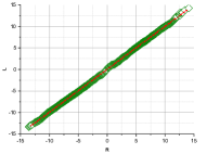
(a) Assumption (a1)

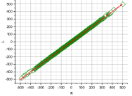
(b) Assumption (a2)

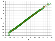
(c) Assumption (a3)

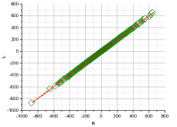
(d) Assumption (a4)

Figure 5: Validation of Assumption 1 using QQ-plots (if two compared distributions are similar, the points will approximately lie on the identity line)

Step 1: Starting from Lines 5-6 of Tab. II, we define $D_{\mathsf{z}}^{-,t}\triangleq\mathbb{E}[z_{0}\hat{\mu}_{\mathsf{z}}^{-,t}]$, $F_{\mathsf{z}}^{-,t}\triangleq\mathbb{E}[(\hat{\mu}_{\mathsf{z}}^{-,t})^{2}]$, $\hat{\mathtt{v}}_{\mathsf{z},1}^{-,t}\triangleq\mathbb{E}[\hat{v}_{\mathsf{z},1}^{-,t}]$, $\hat{\mathtt{v}}_{\mathsf{z},0}^{-,t}\triangleq\mathbb{E}[\hat{v}_{\mathsf{z},0}^{-,t}]$.

Step 2: Substituting Lines 7-9 of Tab. II into (a3), we obtain

$$-\hat{D}_{\mathsf{2z}}^{t}\mathtt{v}_{\mathsf{z}}^{-,t}= \mathtt{v}_{\mathsf{z}}^{-,t}D_{\mathsf{z}}^{-,t}/(C_{\mathsf{z}}\hat{\mathtt{v}}_{\mathsf{z}}^{-,t})+\mathtt{v}_{\mathsf{z}}^{-,t}\hat{D}_{\mathsf{1z}}^{t},$$

$$-\hat{F}_{\mathsf{2z}}^{t}(\mathtt{v}_{\mathsf{z}}^{-,t})^{2}= (\mathtt{v}_{\mathsf{z}}^{-,t})^{2}F_{\mathsf{z}}^{-,t}/(\hat{\mathtt{v}}_{\mathsf{z}}^{-,t})^{2}-(\mathtt{v}_{\mathsf{z}}^{-,t}D_{\mathsf{z}}^{-,t})^{2}/[C_{\mathsf{z}}(\hat{\mathtt{v}}_{\mathsf{z}}^{-,t})^{2}]-$$

$$(\mathtt{v}_{\mathsf{z}}^{-,t})^{2}\hat{F}_{\mathsf{1z}}^{t}-2(\mathtt{v}_{\mathsf{z}}^{-,t})^{2}\sqrt{-\hat{F}_{\mathsf{1z}}^{t}}/\hat{\mathtt{v}}_{\mathsf{z}}^{-,t}\mathbb{E}[(\hat{\bm{\mu}}_{\mathsf{z}}^{-,t})^{\mathsf{T}}\bm{U}\bm{\xi}_{\mathsf{1z}}^{t}/M]$$

$$\overset{\text{(a)}}{=} (\mathtt{v}_{\mathsf{z}}^{-,t})^{2}F_{\mathsf{z}}^{-,t}/(\hat{\mathtt{v}}_{\mathsf{z}}^{-,t})^{2}-(\mathtt{v}_{\mathsf{z}}^{-,t}D_{\mathsf{z}}^{-,t})^{2}/[C_{\mathsf{z}}(\hat{\mathtt{v}}_{\mathsf{z}}^{-,t})^{2}]+(\mathtt{v}_{\mathsf{z}}^{-,t})^{2}\hat{F}_{\mathsf{1z}}^{t},$$

where (a) follows the Stein’s lemma . Then, we get $\mathtt{v}_{\mathsf{z},0}^{-,t}$, $\mathtt{v}_{\mathsf{z}}^{-,t}$, $\hat{D}_{\mathsf{2z}}^{t}$, and $\hat{F}_{\mathsf{2z}}^{t}$ as Lines 12-15 of Tab. III.

Step 3: Substituting (a2) and (a3) into Lines 10-12 of Tab. II, we obtain

$$\hat{\bm{C}}_{\mathsf{x}}^{-,t}= (1/\mathtt{v}_{\mathsf{x}}^{+,t}\bm{I}_{N}+1/\mathtt{v}_{\mathsf{z}}^{-,t}\bm{H}^{\mathsf{T}}\bm{H})^{-1}=\bm{V}(1/\mathtt{v}_{\mathsf{x}}^{+,t}\bm{I}_{N}+1/\mathtt{v}_{\mathsf{z}}^{-,t}\bm{S}^{\mathsf{T}}\bm{S})^{-1}\bm{V}^{\mathsf{T}},$$

$$\hat{\bm{\mu}}_{\mathsf{x}}^{-,t}= \hat{\bm{C}}_{\mathsf{x}}^{-,t}(1/\mathtt{v}_{\mathsf{x}}^{+,t}\bm{\mu}_{\mathsf{x}}^{+,t}+1/\mathtt{v}_{\mathsf{z}}^{-,t}\bm{H}^{\mathsf{T}}\bm{\mu}_{\mathsf{z}}^{-,t})$$

$$= \bm{V}(1/\mathtt{v}_{\mathsf{x}}^{+,t}\bm{I}_{N}+1/\mathtt{v}_{\mathsf{z}}^{-,t}\bm{S}^{\mathsf{T}}\bm{S})^{-1}[(-\hat{D}_{\mathsf{2x}}^{t}-\hat{D}_{\mathsf{2z}}^{t}\bm{S}^{\mathsf{T}}\bm{S})\bm{V}^{\mathsf{T}}\bm{x}_{0}+\sqrt{-\hat{F}_{\mathsf{2x}}^{t}}\bm{\xi}_{\mathsf{2x}}^{t}+\sqrt{-\hat{F}_{\mathsf{2z}}^{t}}\bm{S}^{\mathsf{T}}\bm{U}^{\mathsf{T}}\bm{\xi}_{\mathsf{2z}}^{t}],$$

and define $D_{\mathsf{x}}^{-,t}\triangleq\mathbb{E}[\bm{x}_{0}^{\mathsf{T}}\hat{\bm{\mu}}_{\mathsf{x}}^{-,t}/N]$, $F_{\mathsf{x}}^{-,t}\triangleq\mathbb{E}[\|\hat{\bm{\mu}}_{\mathsf{x}}^{-,t}\|_{2}^{2}/N]$, $\hat{\mathtt{v}}_{\mathsf{x},0}^{-,t}\triangleq\mathbb{E}[\mathsf{Tr}(\hat{\bm{C}}_{\mathsf{x},0}^{-,t})/N]$, and $\hat{\mathtt{v}}_{\mathsf{x}}^{-,t}\triangleq\mathbb{E}[\mathsf{Tr}(\hat{\bm{C}}_{\mathsf{x}}^{-,t})/N]$.

Step 4: Substituting Lines 15-18 into (a1), we obtain

$$-\hat{D}_{\mathsf{1x}}^{t}\mathtt{v}_{\mathsf{x}}^{-,t}= \frac{\mathtt{v}_{\mathsf{x}}^{-,t}D_{\mathsf{x}}^{-,t}}{C_{\mathsf{x}}\hat{\mathtt{v}}_{\mathsf{x}}^{-,t}}+\mathtt{v}_{\mathsf{x}}^{-,t}\hat{D}_{\mathsf{2x}}^{t},$$

$$-\hat{F}_{\mathsf{1x}}^{t}(\mathtt{v}_{\mathsf{x}}^{-,t})^{2}= \frac{(\mathtt{v}_{\mathsf{x}}^{-,t})^{2}F_{\mathsf{x}}^{-,t}}{(\hat{\mathtt{v}}_{\mathsf{x}}^{-,t})^{2}}+\frac{(\mathtt{v}_{\mathsf{x}}^{-,t}D_{\mathsf{x}}^{-,t})^{2}}{C_{\mathsf{x}}(\hat{\mathtt{v}}_{\mathsf{x}}^{-,t})^{2}}+(\mathtt{v}_{\mathsf{x}}^{-,t})^{2}\hat{F}_{\mathsf{2x}}^{t}.$$

Together with $\mathtt{v}_{\mathsf{x},0}^{-,t}$ and $\mathtt{v}_{\mathsf{x}}^{-,t}$ in Tab. III, we have $\hat{D}_{\mathsf{1x}}^{t}$ and $\hat{F}_{\mathsf{1x}}^{t}$.

Step 5: We now analyze Lines 19-20 of Tab. II by defining $D_{\mathsf{x}}^{+,t+1}\triangleq\mathbb{E}[\bm{x}_{0}^{\mathsf{T}}\hat{\bm{\mu}}_{\mathsf{x}}^{+,t+1}/N]$, $F_{\mathsf{x}}^{+,t+1}\triangleq\mathbb{E}[\|\hat{\bm{\mu}}_{\mathsf{x}}^{+,t+1}\|_{2}^{2}/N]$, $\hat{\mathtt{v}}_{\mathsf{x},1}^{+,t+1}\triangleq\mathbb{E}[\hat{v}_{\mathsf{x},1}^{+,t+1}]$, and $\hat{\mathtt{v}}_{\mathsf{x},0}^{+,t+1}\triangleq\mathbb{E}[\hat{v}_{\mathsf{x},0}^{+,t+1}]$.

Step 6: Similar to Step 4, we substitute Lines 21-23 of Tab. II into (a2) and obtain $\hat{D}_{\mathsf{2x}}^{t+1}$ and $\hat{F}_{\mathsf{2x}}^{t+1}$.

Step 7: Similar to Step 3, we first rewrite Lines 27-29 into

$$\hat{\bm{C}}_{\mathsf{z}}^{+,t+1}= \bm{H}\hat{\bm{C}}_{\tilde{\mathsf{x}}}^{+,t+1}\bm{H}^{\mathsf{T}}=\bm{U}\bm{S}(1/\mathtt{v}_{\mathsf{x}}^{+,t+1}\bm{I}_{N}+1/\mathtt{v}_{\mathsf{z}}^{-,t}\bm{S}^{\mathsf{T}}\bm{S})^{-1}\bm{S}^{\mathsf{T}}\bm{U}^{\mathsf{T}},$$

$$\hat{\bm{\mu}}_{\mathsf{z}}^{+,t+1}= \bm{H}\hat{\bm{\mu}}_{\tilde{\mathsf{x}}}^{+,t+1}$$

$$= \bm{U}\bm{S}(1/\mathtt{v}_{\mathsf{x}}^{+,t+1}\bm{I}_{N}+1/\mathtt{v}_{\mathsf{z}}^{-,t}\bm{S}^{\mathsf{T}}\bm{S})^{-1}[(-\hat{D}_{\mathsf{2x}}^{t+1}-\hat{D}_{\mathsf{2z}}^{t}\bm{S}^{\mathsf{T}}\bm{S})\bm{V}^{\mathsf{T}}\bm{x}_{0}+\sqrt{-\hat{F}_{\mathsf{2x}}^{t+1}}\bm{\xi}_{\mathsf{2x}}^{t+1}+$$

$$\sqrt{-\hat{F}_{\mathsf{2z}}^{t}}\bm{S}^{\mathsf{T}}\bm{U}^{\mathsf{T}}\bm{\xi}_{\mathsf{2z}}^{t}].$$

Then, we define $\hat{\mathtt{v}}_{\mathsf{z},0}^{+,t+1}\triangleq\mathbb{E}[\mathsf{Tr}(\hat{\bm{C}}_{\mathsf{z}}^{+,t+1})/M]$, $\hat{\mathtt{v}}_{\mathsf{z}}^{+,t+1}\triangleq\mathbb{E}[\mathsf{Tr}(\hat{\bm{C}}_{\mathsf{z}}^{+,t+1})/M]$, $D_{\mathsf{z}}^{+,t+1}\triangleq\mathbb{E}[\bm{z}_{0}^{\mathsf{T}}\hat{\bm{\mu}}_{\mathsf{z}}^{+,t+1}/M]$, and $F_{\mathsf{z}}^{+,t+1}\triangleq\mathbb{E}[\|\hat{\bm{\mu}}_{\mathsf{z}}^{+,t+1}\|_{2}^{2}/M]$.

Step 8: Similar to Step 2, we substitute Lines 32-34 into (a4) and obtain$\hat{D}_{\mathsf{1z}}^{t+1}$ and $\hat{F}_{\mathsf{1z}}^{t+1}$.

Proposition 3 (State Evolution).

The state evolution of VASP is given in Tab. III, whose fixed point equations perfectly match the 1RSB saddle point equations given in Proposition 1.

TABLE III: The SE Equations of VASP

To see the correspondence between the SE fixed point and the 1RSB saddle point equations, we derive the former ones by taking these steps on Tab. III:

• Omit the iteration index $t$ and $t+1$;

• Merge Lines 12-15 into Lines 40-43 and obtain $\hat{\mathtt{v}}_{\mathsf{z},0}^{-}=\hat{\mathtt{v}}_{\mathsf{z},0}^{+}$, $\hat{\mathtt{v}}_{\mathsf{z}}^{-}=\hat{\mathtt{v}}_{\mathsf{z}}^{+}$, $D_{\mathsf{z}}^{-}=D_{\mathsf{z}}^{+}$, and $F_{\mathsf{z}}^{-}=F_{\mathsf{z}}^{+}$;

• Define $D_{\mathsf{z}}\triangleq D_{\mathsf{z}}^{-}$, $F_{\mathsf{z}}\triangleq F_{\mathsf{z}}^{-}$, $G_{\mathsf{z}}\triangleq\hat{\mathtt{v}}_{\mathsf{z},0}^{-}+F_{\mathsf{z}}$, and $H_{\mathsf{z}}\triangleq(\hat{\mathtt{v}}_{\mathsf{z}}^{-}-\hat{\mathtt{v}}_{\mathsf{z},0}^{-})/L$;

• Merge Lines 20-23 into Lines 32-35 and define $D_{\mathsf{x}}$, $F_{\mathsf{x}}$, $G_{\mathsf{x}}$, and $H_{\mathsf{x}}$ similarly as the above.

Then, we see the SE fixed point equations of VASP match exactly with 1RSB saddle point equations of the 1RSB free energy given in Tab. I of Proposition 1.

Recall that our saddle point equations are equivalent to Kabashima’s 1RSB replica result [1] that corresponds to the optimal estimator (3) in the model-mismatch setting with a rotation-invariant measurement matrix. It can be implied from Proposition 3 our VASP computes exactly the optimal estimator (3) in the large system limit, as long as the 1RSB ansatz is valid and VASP converges to the SE fixed point. VAMP also computes the optimal estimator (3) but limited to the RS ansatz [1]. RSB plays a crucial role in characterizing a fundamental limit of VAMP. As pointed out in [27, 45, 1], RSB appears when the postulated likelihood $q_{\mathsf{y|z}}(\bm{y}|\bm{z}_{0})$ differs from the actual likelihood $p_{\mathsf{y|z}}(\bm{y}|\bm{z}_{0})$ and the log-posterior $-\sum_{a=1}^{M}\log p(y_{a}|z_{0,a})-\sum_{i=1}^{N}\log p(x_{0,i})$ is non-convex, although it is difficult to know a priori what degree of model-mismatch or non-convexity causes the RSB. RSB prevents VAMP from converging because there are so many fixed points [1]: the number of VAMP fixed points grows exponentially in $N$, due to the combination of the model-mismatch and non-convexity of log-posterior. An analysis for the number of fixed point was believed to be demanding because of a very complicated calculation [1]. So far, the extension of VAMP to the RSB cases remains an open problem. In this context, the VASP above provides an answer to the question: it extends VAMP in computing exactly the optimal estimator (3) to cases, where the 1RSB ansatz is valid, including RS as a special case.

V Validation and Discussion

This section validates Propositions 2 and 3 using two applications from engineering fields, i.e., phase retrieval for image processing and MIMO detection for wireless communications, both in the model-mismatch setting. We consider the MAP optimal estimator (3), i.e., $\beta\to+\infty$, in which case the computation for Line 5 and Line 19 of Algorithm II particularizes into Lines 11-18 and 20-22 of Tab. IV, with the detail given in the supplementary material of this paper. Also, we adopt the (left) rotation invariant measurement matrix constructed by the Kronecker correlation model [46]: $\bm{H}=\bm{F}\bm{R}^{\frac{1}{2}}$, where $\bm{R}$ is a deterministic matrix whose $(i,j)$-th element is $R^{(i,j)}=\rho^{|i-j|},\rho\in[0,1)$, and $\bm{F}$ is drawn from a Gaussian ensemble having i.i.d., zero-mean, and unit-variance elements. The Julia code for the simulations here can be found at https://github.com/PeiKaLunCi/VASP_JL.

V-A Phase Retrieval

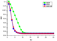
(a) i.i.d. case

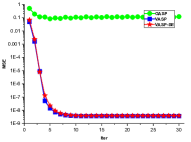
(b) Correlated case

Figure 6: Per-iteration MSE of GASP, VASP and VASP’s SE.

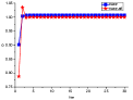
(a) $D_{\mathsf{x}}^{+,t}$

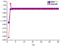
(b) $F_{\mathsf{x}}^{+,t}$

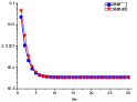
(c) $H_{\mathsf{x}}^{+,t}$

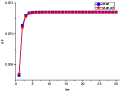
(d) $G_{\mathsf{x}}^{+,t}-F_{\mathsf{x}}^{+,t}$

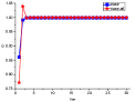
(e) $D_{\mathsf{x}}^{+,t}$

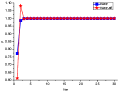
(f) $F_{\mathsf{x}}^{+,t}$

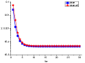
(g) $H_{\mathsf{x}}^{+,t}$

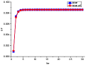
(h) $G_{\mathsf{x}}^{+,t}-F_{\mathsf{x}}^{+,t}$

Figure 7: Per-iteration behavior of macroscopic variables $D_{\mathsf{x}}^{+,t}$, $F_{\mathsf{x}}^{+,t}$, $G_{\mathsf{x}}^{+,t}$ and $H_{\mathsf{x}}^{+,t}$. (a)-(d): i.i.d., (e)-(h): correlated.

In the application to phase retrieval [47, 48], the generation process is specialized as

$$p(x_{0,i})= \mathsf{N}[x_{0,i}|0,1],$$

$$p(y_{a}|z_{0,a})= \delta[y_{a}-\mathsf{abs}(z_{0,a})],$$

while the (mismatched) inference process is specialized as

$$q(x_{0,i})= \mathsf{N}[x_{0,i}|0,1/{\lambda}],$$

$$q(y_{a}|z_{0,a})= \mathsf{N}[y_{a}|\mathsf{abs}(z_{0,a}),v_{\mathsf{w}}].$$

Throughout this subsection, we fix the parameters as $T=30$, $N=1000$, and $v_{\mathsf{w}}=1/2$. For the rotation invariant (correlated) case of the measurement matrix $\bm{H}$, we use $\rho=0.4$, while in the i.i.d. case, $\rho=0$. Then, we have these remarks:

(i) Per-iteration behavior of VASP: Given $\alpha=8$, $L=10$, and $\lambda=10^{-5}$, we compare the MSE of VASP with GASP [23]. As shown in Fig. 6, VASP in Proposition 2 is highly effective in the model-mismatch setting: for the i.i.d. case, VASP converges in only a few iterations, which is much faster than GASP, although their fixed points are exactly the same; for the correlated case, VASP outperforms GASP significantly. Moreover, in both cases, the SE in Proposition 3 is observed to capture the dynamical behavior of VASP perfectly.

(ii) Macroscopic analysis: A closer look into the macroscopic variables of the SE, including $D_{\mathsf{x}}^{+,t}$, $F_{\mathsf{x}}^{+,t}$, $G_{\mathsf{x}}^{+,t}$, and $H_{\mathsf{x}}^{+,t}$, further suggests the VASP trajectories are in great accordance with those of the SE, as shown in Fig. 7.

(iii) Robustness to parameter change: We keep the above setting and vary the parameters of $\alpha$, $L$, and $\lambda$, alternatively. Fig. 8 shows that VASP is robust to such parameter change, and the SE remains valid in all cases considered. It is also observed increasing $L$ can boost VASP’s performance. As mentioned in [23], $L$ allows to select the contributions of different families of states. Specifically, $L$ acts as an inverse temperature coupled to the internal free energy of the states: increasing $L$ selects families of states with lower complexity and lower free energy. However, a theory to support the selection of the most appropriate $L$ is still missing [23].

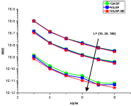
(a) MSEs versus $\alpha$

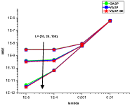
(b) MSEs versus $\lambda$

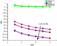
(c) MSEs versus $\alpha$

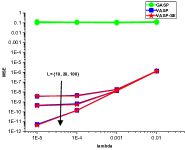
(d) MSEs versus $\lambda$

Figure 8: Robustness to parameter change of $\alpha$, $\lambda$, and $L$. (a)-(b): i.i.d., (c)-(d): correlated.

V-B MIMO Detection

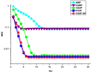
(a) i.i.d. case

(b) Correlated case

Figure 9: Per-iteration MSE of AMP, VAMP, GASP, VASP and VASP’s SE.

In the application to MIMO detection [49], the generation process is specialized as

$$p(x_{0,i})= [\delta(x_{0,i}+a_{\mathsf{T}})+\delta(x_{0,i}-a_{\mathsf{T}})]/2,$$

$$p(y_{a}|z_{a})= \mathsf{N}[y_{a}|z_{a},v_{\mathsf{T}}],$$

while the inference process is specialized as

$$q(x_{0,i})= [\delta(x_{0,i}+a_{\mathsf{F}})+\delta(x_{0,i}-a_{\mathsf{F}})]/2,$$

$$q(y_{a}|z_{a})= \mathsf{N}[y_{a}|z_{a},v_{\mathsf{F}}].$$

Clearly, in this application, the log-posterior for approximate inference is non-convex, thus breaking the RS ansatz [27]. Throughout this subsection, we fix the parameters as $T=30$, $N=5000$, $a_{\mathsf{T}}=a_{\mathsf{F}}=1$, $L=10$, $v_{\mathsf{T}}=0.1$, and $v_{\mathsf{F}}=0.15$. we also use $\rho=0.4$ and $\rho=0$ to model the rotation invariant (correlated) and i.i.d. measurement matrices $\bm{H}$, respectively. Then, we have these remarks:

(i) Superiority over belief propagation algorithms: Fig. 9(a) considers an i.i.d. case. For the i.i.d. case in the model-mismatch setting, Fig. 9(a) demonstrates survey propagation algorithms (including GASP [23] and the proposed VASP) outperforms the belief propagation ones (including AMP [8, 9] and VAMP [18, 5]). For the correlated case, Fig. 9(b), the vector-form message passing (including VAMP [18, 5]) and the proposed VASP) is superior to its scalar-form counterpart (including AMP [8, 9] and GASP [23]). In all cases above, VASP provides the best performance.

(ii) Consistent with macroscopic analysis: In both i.i.d. and correlated cases, the VASP SE can capture exactly the per-iteration MSE of the algorithm, as seen from Fig. 9. In Fig. 10, we also examine the trajectories of VASP through the macroscopic variables of $D_{\mathsf{x}}^{+,t}$, $F_{\mathsf{x}}^{+,t}$, $G_{\mathsf{x}}^{+,t}$, and $H_{\mathsf{x}}^{+,t}$, which shows the VASP trajectories are in excellent accordance with those of the SE.

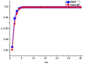
(a) $D_{\mathsf{x}}^{+,t}$ versus iter

(b) $F_{\mathsf{x}}^{+,t}$ versus iter

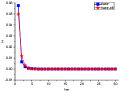
(c) $H_{\mathsf{x}}^{+,t}$ versus iter

(d) $G_{\mathsf{x}}^{+,t}-F_{\mathsf{x}}^{+,t}$ versus iter

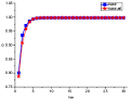
(e) $D_{\mathsf{x}}^{+,t}$ versus iter

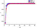
(f) $F_{\mathsf{x}}^{+,t}$ versus iter

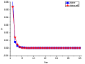
(g) $H_{\mathsf{x}}^{+,t}$ versus iter

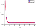
(h) $G_{\mathsf{x}}^{+,t}-F_{\mathsf{x}}^{+,t}$ versus iter

Figure 10: Per-iteration behavior of macroscopic variables $D_{\mathsf{x}}^{+,t}$, $F_{\mathsf{x}}^{+,t}$, $G_{\mathsf{x}}^{+,t}$, and $H_{\mathsf{x}}^{+,t}$. (a)-(d): i.i.d., (e)-(h): correlated.

VI Conclusion

For approximate inference in the GLM involving a rotation-invariant measurement matrix, Kabashima and collaborators had found VAMP is sub-optimal in a model-mismatch setting where RSB occurs. Although they had pointed out a direction for the optimal estimator, i.e., by providing the saddle point equations for the free energy of the optimal estimator under the 1RSB ansatz, it remains an open problem how to achieve this prediction. In this paper, we introduced the VASP algorithm to fill in this gap. We first reformulated the extremum conditions in Kabashima’s replica analysis, and later connects the theoretical equations to the definition of a survey, and finally design a concrete implementation based on survey propagation in a new vector form. The VASP obtained is as computationally efficient as VAMP, and it includes VAMP as a special case. We also derived the SE for VASP, which can capture the per-iteration behavior of the simulated algorithm precisely. The SE fixed point equations was later found perfectly matched with Kabashima’s 1RSB prediction, by which we concluded that VASP converges to the optimal estimator. To see more evidence on our theoretical findings, we carried out extensive simulations and confirmed that VASP generally outperforms other state-of-the-art inference methods.

The authors would like to thank Prof. Carlo Lucibello for many helpful discussions and his sharing of the GASP code.

Appendix A Reformulation of 1RSB Saddle Point Equations

TABLE IV: Summary of notations

The extremum conditions then read [1, eqs. (124)-(126)]:

$$\bm{0}= \bm{\Lambda}_{\mathsf{z}}-\bm{Q}_{\mathsf{z}}^{-1}+\tilde{\bm{Q}}_{\mathsf{z}},$$ (33a)

$$\bm{0}= \bm{\Lambda}_{\mathsf{x}}-\bm{Q}_{\mathsf{x}}^{-1}+\tilde{\bm{Q}}_{\mathsf{x}},$$ (33b)

$$\bm{Q}_{\mathsf{z}}= \frac{1}{\alpha}\mathbb{E}_{\lambda}[\lambda(\bm{\Lambda}_{\mathsf{x}}+\lambda\bm{\Lambda}_{\mathsf{z}})^{-1}],$$ (33c)

$$\bm{Q}_{\mathsf{x}}= \mathbb{E}_{\lambda}[(\bm{\Lambda}_{\mathsf{x}}+\lambda\bm{\Lambda}_{\mathsf{z}})^{-1}],$$ (33d)

$$\bm{Q}_{\mathsf{z}}= \frac{\int{\mathsf{d}y\mathsf{d}\vec{\bm{z}}}\,p(y\bm{1}|\vec{\bm{z}})\mathsf{e}(-\frac{1}{2}\vec{\bm{z}}\tilde{\bm{Q}}_{\mathsf{z}}\vec{\bm{z}}^{\mathsf{T}})\vec{\bm{z}}^{\mathsf{T}}\vec{\bm{z}}}{\int{\mathsf{d}y\mathsf{d}\vec{\bm{z}}}\,p(y\bm{1}|\vec{\bm{z}})\mathsf{e}(-\frac{1}{2}\vec{\bm{z}}\tilde{\bm{Q}}_{\mathsf{z}}\vec{\bm{z}}^{\mathsf{T}})},$$ (33e)

$$\bm{Q}_{\mathsf{x}}= \frac{\int{\mathsf{d}\vec{\bm{x}}}\,\mathsf{e}(-\frac{1}{2}\vec{\bm{x}}\tilde{\bm{Q}}_{\mathsf{x}}\vec{\bm{x}}^{\mathsf{T}})p(\vec{\bm{x}})\vec{\bm{x}}^{\mathsf{T}}\vec{\bm{x}}}{\int{\mathsf{d}\vec{\bm{x}}}\,\mathsf{e}(-\frac{1}{2}\vec{\bm{x}}\tilde{\bm{Q}}_{\mathsf{x}}\vec{\bm{x}}^{\mathsf{T}})p(\vec{\bm{x}})}.$$ (33f)

The 1RSB ansatz says: solutions to the replica extremum condition exhibit the following matrix structure [27, 1, 34]

$$\bm{Q}_{\mathsf{z}}= \mathcal{Q}_{\tau+1,L}(C_{\mathsf{z}},D_{\mathsf{z}},F_{\mathsf{z}},G_{\mathsf{z}},H_{\mathsf{z}}),$$

$$\bm{Q}_{\mathsf{x}}= \mathcal{Q}_{\tau+1,L}(C_{\mathsf{x}},D_{\mathsf{x}},F_{\mathsf{x}},G_{\mathsf{x}},H_{\mathsf{x}}),$$

$$\bm{\Lambda}_{\mathsf{z}}= \mathcal{Q}_{\tau+1,L}(\hat{C}_{\mathsf{2z}},\hat{D}_{\mathsf{2z}},\hat{F}_{\mathsf{2z}},\hat{G}_{\mathsf{2z}},\hat{H}_{\mathsf{2z}}),$$

$$\bm{\Lambda}_{\mathsf{x}}= \mathcal{Q}_{\tau+1,L}(\hat{C}_{\mathsf{2x}},\hat{D}_{\mathsf{2x}},\hat{F}_{\mathsf{2x}},\hat{G}_{\mathsf{2x}},\hat{H}_{\mathsf{2x}}),$$

$$\tilde{\bm{Q}}_{\mathsf{z}}= \mathcal{Q}_{\tau+1,L}(\hat{C}_{\mathsf{1z}},\hat{D}_{\mathsf{1z}},\hat{F}_{\mathsf{1z}},\hat{G}_{\mathsf{1z}},\hat{H}_{\mathsf{1z}}),$$

$$\tilde{\bm{Q}}_{\mathsf{x}}= \mathcal{Q}_{\tau+1,L}(\hat{C}_{\mathsf{1x}},\hat{D}_{\mathsf{1x}},\hat{F}_{\mathsf{1x}},\hat{G}_{\mathsf{1x}},\hat{H}_{\mathsf{1x}}),$$

where $\mathcal{Q}_{\tau+1,L}(C,D,F,G,H)\triangleq\left[\begin{array}[]{cc}C&D\vec{\bm{1}}_{\tau}\\ D\bm{1}_{\tau}&\mathcal{A}_{\tau,L}(F,G,H)\\ \end{array}\right]$ and $\mathcal{A}_{\tau,L}(F,G,H)\triangleq F\mathbb{1}_{\tau}+(G-F)\bm{I}_{\tau}+H\bm{I}_{\frac{\tau}{L}}\otimes\mathbb{1}_{L}$.

Lemma 1 (Decomposition Formula).

A matrix $\mathcal{Q}_{\tau+1,L}$ in the 1RSB form can be decomposed as [25]

$$\mathcal{Q}_{\tau+1,L}= \bm{F}\bm{D}_{\mathsf{q}}\bm{F}^{\mathsf{H}},$$

$$\bm{F}\triangleq \left[\begin{array}[]{cccc}1&\\ &\bm{F}_{\tau/L}/\sqrt{\tau/L}\otimes\bm{F}_{L}/\sqrt{L}\\ \end{array}\right],$$

$$\bm{D}_{\mathsf{q}}^{(i,j)}\triangleq \begin{cases}C&i=j=0\\ \sqrt{\tau}D&(i=0,\,j=1)\,\text{or}\,(i=1,\,j=0)\\ \bm{D}_{\mathsf{a}}^{(i-1,i-1)}&(i\geq 1,j\geq 1,i=j)\\ 0&\text{other}\\ \end{cases},$$

where $\bm{D}_{\mathsf{a}}\triangleq\mathsf{D}[(G-F)\bm{1}_{\tau}+LH\bm{1}_{\tau/L}\otimes\bm{e}_{L}+\tau F\bm{e}_{\tau}]$ and $\bm{F}_{L}$ represents an $L\times L$ discrete Fourier transform matrix, with $\bm{F}_{L}^{(m,n)}$ defined as $\mathsf{e}[-\mathbb{j}2\pi(m-1)(n-1)/L]/\sqrt{L}$.

We next take steps to reformulate the 1RSB saddle point equations, but we start from the extremum conditions (33).

(S1) Under the 1RSB ansatz, (33a)-(33b) are specified as:

$$0= \hat{C}_{\mathsf{1x}}+\hat{C}_{\mathsf{2x}}-\frac{1}{C_{\mathsf{x}}},$$ (34)

$$0= \hat{D}_{\mathsf{1x}}+\hat{D}_{\mathsf{2x}}+\frac{D_{\mathsf{x}}}{C_{\mathsf{x}}(G_{\mathsf{x}}-F_{\mathsf{x}}+LH_{\mathsf{x}})},$$ (35)

$$0= \hat{F}_{\mathsf{1x}}+\hat{F}_{\mathsf{2x}}-\frac{D_{\mathsf{x}}^{2}}{C_{\mathsf{x}}(G_{\mathsf{x}}-F_{\mathsf{x}}+LH_{\mathsf{x}})^{2}}+\frac{F_{\mathsf{x}}}{(G_{\mathsf{x}}-F_{\mathsf{x}}+LH_{\mathsf{x}})^{2}},$$ (36)

$$0= \hat{G}_{\mathsf{1x}}+\hat{G}_{\mathsf{2x}}-\frac{D_{\mathsf{x}}^{2}}{C_{\mathsf{x}}(G_{\mathsf{x}}-F_{\mathsf{x}}+LH_{\mathsf{x}})^{2}}+\frac{F_{\mathsf{x}}}{(G_{\mathsf{x}}-F_{\mathsf{x}}+LH_{\mathsf{x}})^{2}}-\frac{1}{G_{\mathsf{x}}-F_{\mathsf{x}}},$$ (37)

$$0= \hat{H}_{\mathsf{1x}}+\hat{H}_{\mathsf{2x}}-\frac{1}{L}(\frac{1}{G_{\mathsf{x}}-F_{\mathsf{x}}+LH_{\mathsf{x}}}-\frac{1}{G_{\mathsf{x}}-F_{\mathsf{x}}}),$$ (38)

$$0= \hat{C}_{\mathsf{1z}}+\hat{C}_{\mathsf{2z}}-\frac{1}{C_{\mathsf{z}}},$$ (39)

$$0= \hat{D}_{\mathsf{1z}}+\hat{D}_{\mathsf{2z}}+\frac{D_{\mathsf{z}}}{C_{\mathsf{z}}(G_{\mathsf{z}}-F_{\mathsf{z}}+LH_{\mathsf{z}})},$$ (40)

$$0= \hat{F}_{\mathsf{1z}}+\hat{F}_{\mathsf{2z}}-\frac{D_{\mathsf{z}}^{2}}{C_{\mathsf{z}}(G_{\mathsf{z}}-F_{\mathsf{z}}+LH_{\mathsf{z}})^{2}}+\frac{F_{\mathsf{z}}}{(G_{\mathsf{z}}-F_{\mathsf{z}}+LH_{\mathsf{z}})^{2}},$$ (41)

$$0= \hat{G}_{\mathsf{1z}}+\hat{G}_{\mathsf{2z}}-\frac{D_{\mathsf{z}}^{2}}{C_{\mathsf{z}}(G_{\mathsf{z}}-F_{\mathsf{z}}+LH_{\mathsf{z}})^{2}}+\frac{F_{\mathsf{z}}}{(G_{\mathsf{z}}-F_{\mathsf{z}}+LH_{\mathsf{z}})^{2}}-\frac{1}{G_{\mathsf{z}}-F_{\mathsf{z}}},$$ (42)

$$0= \hat{H}_{\mathsf{1z}}+\hat{H}_{\mathsf{2z}}-\frac{1}{L}(\frac{1}{G_{\mathsf{z}}-F_{\mathsf{z}}+LH_{\mathsf{z}}}-\frac{1}{G_{\mathsf{z}}-F_{\mathsf{z}}}).$$ (43)

(S2) Similarly, (33c)-(33d) produce

$$C_{\mathsf{x}}= \mathbb{E}_{\lambda}[\frac{1}{\hat{C}_{\mathsf{2x}}+\lambda\hat{C}_{\mathsf{2z}}}],$$ (44)

$$D_{\mathsf{x}}= -\mathbb{E}_{\lambda}[\frac{\hat{D}_{\mathsf{2x}}+\lambda\hat{D}_{\mathsf{2z}}}{(\hat{C}_{\mathsf{2x}}+\lambda\hat{C}_{\mathsf{2z}})[(\hat{G}_{\mathsf{2x}}-\hat{F}_{\mathsf{2x}}+L\hat{H}_{\mathsf{2x}})+\lambda(\hat{G}_{\mathsf{2z}}-\hat{F}_{\mathsf{2z}}+L\hat{H}_{\mathsf{2z}})]}],$$ (45)

$$F_{\mathsf{x}}= \mathbb{E}_{\lambda}[\frac{(\hat{D}_{\mathsf{2x}}+\lambda\hat{D}_{\mathsf{2z}})^{2}}{(\hat{C}_{\mathsf{2x}}+\lambda\hat{C}_{\mathsf{2z}})[(\hat{G}_{\mathsf{2x}}-\hat{F}_{\mathsf{2x}}+L\hat{H}_{\mathsf{2x}})+\lambda(\hat{G}_{\mathsf{2z}}-\hat{F}_{\mathsf{2z}}+L\hat{H}_{\mathsf{2z}})]^{2}}]-$$

$$\mathbb{E}_{\lambda}[\frac{\hat{F}_{\mathsf{2x}}+\lambda\hat{F}_{\mathsf{2z}}}{[(\hat{G}_{\mathsf{2x}}-\hat{F}_{\mathsf{2x}}+L\hat{H}_{\mathsf{2x}})+\lambda(\hat{G}_{\mathsf{2z}}-\hat{F}_{\mathsf{2z}}+L\hat{H}_{\mathsf{2z}})]^{2}}],$$ (46)

$$G_{\mathsf{x}}= F_{\mathsf{x}}+\mathbb{E}_{\lambda}[\frac{1}{(\hat{G}_{\mathsf{2x}}-\hat{F}_{\mathsf{2x}})+\lambda(\hat{G}_{\mathsf{2z}}-\hat{F}_{\mathsf{2z}})}],$$ (47)

$$H_{\mathsf{x}}= \frac{1}{L}\{\mathbb{E}_{\lambda}[\frac{1}{(\hat{G}_{\mathsf{2x}}-\hat{F}_{\mathsf{2x}}+L\hat{H}_{\mathsf{2x}})+\lambda(\hat{G}_{\mathsf{2z}}-\hat{F}_{\mathsf{2z}}+L\hat{H}_{\mathsf{2z}})}]-\mathbb{E}_{\lambda}[\frac{1}{(\hat{G}_{\mathsf{2x}}-\hat{F}_{\mathsf{2x}})+\lambda(\hat{G}_{\mathsf{2z}}-\hat{F}_{\mathsf{2z}})}]\},$$ (48)

$$C_{\mathsf{z}}= \frac{1}{\alpha}\mathbb{E}_{\lambda}[\frac{\lambda}{\hat{C}_{\mathsf{2x}}+\lambda\hat{C}_{\mathsf{2z}}}],$$ (49)

$$D_{\mathsf{z}}= -\frac{1}{\alpha}\mathbb{E}_{\lambda}[\frac{\lambda(\hat{D}_{\mathsf{2x}}+\lambda\hat{D}_{\mathsf{2z}})}{(\hat{C}_{\mathsf{2x}}+\lambda\hat{C}_{\mathsf{2z}})[(\hat{G}_{\mathsf{2x}}-\hat{F}_{\mathsf{2x}}+L\hat{H}_{\mathsf{2x}})+\lambda(\hat{G}_{\mathsf{2z}}-\hat{F}_{\mathsf{2z}}+L\hat{H}_{\mathsf{2z}})]}],$$ (50)

$$F_{\mathsf{z}}= \frac{1}{\alpha}\mathbb{E}_{\lambda}[\frac{\lambda(\hat{D}_{\mathsf{2x}}+\lambda\hat{D}_{\mathsf{2z}})^{2}}{(\hat{C}_{\mathsf{2x}}+\lambda\hat{C}_{\mathsf{2z}})[(\hat{G}_{\mathsf{2x}}-\hat{F}_{\mathsf{2x}}+L\hat{H}_{\mathsf{2x}})+\lambda(\hat{G}_{\mathsf{2z}}-\hat{F}_{\mathsf{2z}}+L\hat{H}_{\mathsf{2z}})]^{2}}]-$$

$$\frac{1}{\alpha}\mathbb{E}_{\lambda}[\frac{\lambda(\hat{F}_{\mathsf{2x}}+\lambda\hat{F}_{\mathsf{2z}})}{[(\hat{G}_{\mathsf{2x}}-\hat{F}_{\mathsf{2x}}+L\hat{H}_{\mathsf{2x}})+\lambda(\hat{G}_{\mathsf{2z}}-\hat{F}_{\mathsf{2z}}+L\hat{H}_{\mathsf{2z}})]^{2}}],$$ (51)

$$G_{\mathsf{z}}= F_{\mathsf{z}}+\frac{1}{\alpha}\mathbb{E}_{\lambda}[\frac{\lambda}{(\hat{G}_{\mathsf{2x}}-\hat{F}_{\mathsf{2x}})+\lambda(\hat{G}_{\mathsf{2z}}-\hat{F}_{\mathsf{2z}})}],$$ (52)

$$H_{\mathsf{z}}= \frac{1}{\alpha}\frac{1}{L}\{\mathbb{E}_{\lambda}[\frac{\lambda}{(\hat{G}_{\mathsf{2x}}-\hat{F}_{\mathsf{2x}}+L\hat{H}_{\mathsf{2x}})+\lambda(\hat{G}_{\mathsf{2z}}-\hat{F}_{\mathsf{2z}}+L\hat{H}_{\mathsf{2z}})}]-\mathbb{E}_{\lambda}[\frac{\lambda}{(\hat{G}_{\mathsf{2x}}-\hat{F}_{\mathsf{2x}})+\lambda(\hat{G}_{\mathsf{2z}}-\hat{F}_{\mathsf{2z}})}]\}.$$ (53)

(S3) The reformulation of (33f) starts from the expansion of $\vec{\bm{x}}\tilde{\bm{Q}}_{x}\vec{\bm{x}}^{\mathsf{T}}$ detailed as below:

$$\vec{\bm{x}}\tilde{\bm{Q}}_{x}\vec{\bm{x}}^{\mathsf{T}}\overset{\text{(a)}}{=} \vec{\bm{x}}\bm{F}\bm{D}_{\mathsf{x}}\bm{F}^{\mathsf{H}}\vec{\bm{x}}^{\mathsf{T}}$$

$$= \sum_{i=0}^{\tau}{}\sum_{j=0}^{\tau}{}\vec{\bm{x}}\bm{f}_{i}\bm{D}_{\mathsf{x}}^{(i,j)}\bm{f}_{j}^{\mathsf{H}}\vec{\bm{x}}^{\mathsf{T}}$$

$$= \hat{C}_{\mathsf{1x}}\vec{\bm{x}}\bm{f}_{0}\bm{f}_{0}^{\mathsf{H}}\vec{\bm{x}}^{\mathsf{T}}+2\sqrt{\tau}\hat{D}_{\mathsf{1x}}\vec{\bm{x}}\bm{f}_{1}\bm{f}_{0}^{\mathsf{H}}\vec{\bm{x}}^{\mathsf{T}}+\tau\hat{F}_{\mathsf{1x}}\vec{\bm{x}}\bm{f}_{1}\bm{f}_{1}^{\mathsf{H}}\vec{\bm{x}}^{\mathsf{T}}+(\hat{G}_{\mathsf{1x}}-\hat{F}_{\mathsf{1x}})\sum_{i=1}^{\tau}{}\vec{\bm{x}}\bm{f}_{i}\bm{f}_{i}^{\mathsf{H}}\vec{\bm{x}}^{\mathsf{T}}+$$

$$L\hat{H}_{\mathsf{1x}}\sum_{i=1}^{\frac{\tau}{L}}{}\vec{\bm{x}}\bm{f}_{L(i-1)+2}\bm{f}_{L(i-1)+2}^{\mathsf{H}}\vec{\bm{x}}^{\mathsf{T}}$$

$$= (\hat{C}_{\mathsf{1x}}-\frac{\hat{D}_{\mathsf{1x}}^{2}}{\hat{F}_{\mathsf{1x}}})x_{0}^{2}+(\hat{G}_{\mathsf{1x}}-\hat{F}_{\mathsf{1x}})\sum_{i=1}^{\tau}\tilde{x}_{i}^{2}+(\frac{\hat{D}_{\mathsf{1x}}}{\sqrt{\hat{F}_{\mathsf{1x}}}}x_{0}+\sum_{i=1}^{\tau}\sqrt{\hat{F}_{\mathsf{1x}}}\tilde{x}_{i})^{2}+\hat{H}_{\mathsf{1x}}\sum_{i=1}^{\frac{\tau}{L}}(\sum_{j=1}^{L}\tilde{x}_{L(i-1)+j+1})^{2},$$

where (a) follows from Lemma of decomposition formula, then $\mathsf{e}(-\frac{1}{2}\vec{\bm{x}}\tilde{\bm{Q}}_{x}\vec{\bm{x}}^{\mathsf{T}})$ is evaluated as:

$$\mathsf{e}(-\frac{1}{2}\vec{\bm{x}}\tilde{\bm{Q}}_{x}\vec{\bm{x}}^{\mathsf{T}})$$

$$= \mathsf{e}[-\frac{1}{2}(\hat{C}_{\mathsf{1x}}-\frac{\hat{D}_{\mathsf{1x}}^{2}}{\hat{F}_{\mathsf{1x}}})x_{0}^{2}]\mathsf{e}[-\frac{1}{2}(\hat{G}_{\mathsf{1x}}-\hat{F}_{\mathsf{1x}})\sum_{i=1}^{\tau}\tilde{x}_{i}^{2}]\mathsf{e}[-\frac{1}{2}(\frac{\hat{D}_{\mathsf{1x}}}{\sqrt{\hat{F}_{\mathsf{1x}}}}x_{0}+\sum_{i=1}^{\tau}\sqrt{\hat{F}_{\mathsf{1x}}}\tilde{x}_{i})^{2}]\times$$

$$\mathsf{e}[-\frac{1}{2}\hat{H}_{\mathsf{1x}}\sum_{i=1}^{\frac{\tau}{L}}(\sum_{j=1}^{L}\tilde{x}_{L(i-1)+j+1})^{2}]$$

$$\overset{\text{(b)}}{=} \mathsf{e}[-\frac{1}{2}(\hat{C}_{\mathsf{1x}}-\frac{\hat{D}_{\mathsf{1x}}^{2}}{\hat{F}_{\mathsf{1x}}})x_{0}^{2}]\mathsf{e}[-\frac{1}{2}(\hat{G}_{\mathsf{1x}}-\hat{F}_{\mathsf{1x}})\sum_{i=1}^{\tau}\tilde{x}_{i}^{2}]\sqrt{\frac{\eta_{\mathsf{x}}}{\pi}}\int{\mathsf{d}\mu_{\mathsf{x}}}\,\mathsf{e}[-\eta_{\mathsf{x}}\mu_{\mathsf{x}}^{2}+2\mathbb{j}\sqrt{\eta_{\mathsf{x}}}\frac{1}{\sqrt{2}}(\frac{\hat{D}_{\mathsf{1x}}}{\sqrt{\hat{F}_{\mathsf{1x}}}}x_{0}+$$

$$\sum_{i=1}^{\tau}\sqrt{\hat{F}_{\mathsf{1x}}}\tilde{x}_{i})\mu_{\mathsf{x}}]\mathsf{e}[-\frac{1}{2}\hat{H}_{\mathsf{1x}}\sum_{i=1}^{\frac{\tau}{L}}(\sum_{j=1}^{L}\tilde{x}_{L(i-1)+j+1})^{2}]$$

$$= \sqrt{\frac{\eta_{\mathsf{x}}}{\pi}}\int{\mathsf{d}\mu_{\mathsf{x}}}\,\mathsf{e}(-\eta_{\mathsf{x}}\mu_{\mathsf{x}}^{2})\mathsf{e}[-\frac{1}{2}(\hat{C}_{\mathsf{1x}}-\frac{\hat{D}_{\mathsf{1x}}^{2}}{\hat{F}_{\mathsf{1x}}})x_{0}^{2}+\frac{\mathbb{j}\sqrt{2\eta_{\mathsf{x}}}\hat{D}_{\mathsf{1x}}}{\sqrt{\hat{F}_{\mathsf{1x}}}}x_{0}\mu_{\mathsf{x}}]\prod_{i=1}^{\frac{\tau}{L}}\mathsf{e}[-\frac{1}{2}(\hat{G}_{\mathsf{1x}}-\hat{F}_{\mathsf{1x}})(\sum_{j=1}^{L}\tilde{x}_{L(i-1)+j+1}^{2})+$$

$$\mathbb{j}\sqrt{2\eta_{\mathsf{x}}\hat{F}_{\mathsf{1x}}}\mu_{\mathsf{x}}(\sum_{j=1}^{L}\tilde{x}_{L(i-1)+j+1})-\frac{1}{2}\hat{H}_{\mathsf{1x}}(\sum_{j=1}^{L}\tilde{x}_{L(i-1)+j+1})^{2}]$$

$$\overset{\text{(c)}}{\propto} \int{\mathsf{d}\mu_{\mathsf{x}}}\,\mathsf{e}(-\eta_{\mathsf{x}}\mu_{\mathsf{x}}^{2})\mathsf{e}[-\frac{1}{2}(\hat{C}_{\mathsf{1x}}-\frac{\hat{D}_{\mathsf{1x}}^{2}}{\hat{F}_{\mathsf{1x}}})x_{0}^{2}+\frac{\mathbb{j}\sqrt{2\eta_{\mathsf{x}}}\hat{D}_{\mathsf{1x}}}{\sqrt{\hat{F}_{\mathsf{1x}}}}x_{0}\mu_{\mathsf{x}}]\prod_{i=1}^{\frac{\tau}{L}}\int{\mathsf{d}\beta}\,\mathsf{N}[\beta|m_{\mathsf{x}},\Delta_{\mathsf{x1}}]\prod_{j=1}^{L}{}\mathsf{N}[\tilde{x}_{L(i-1)+j}|\beta,\Delta_{\mathsf{x0}}],$$

where (b) uses the H-S transform and (c) uses the Gaussian density convolution [40], together with

$$m_{\mathsf{x}}= \frac{\mathbb{j}\sqrt{2\eta_{\mathsf{x}}\hat{F}_{\mathsf{1x}}}\mu_{\mathsf{x}}}{\hat{G}_{\mathsf{1x}}-\hat{F}_{\mathsf{1x}}+L\hat{H}_{\mathsf{1x}}},$$

$$\Delta_{\mathsf{x0}}= \frac{1}{\hat{G}_{\mathsf{1x}}-\hat{F}_{\mathsf{1x}}},$$

$$\Delta_{\mathsf{x1}}= \frac{-\hat{H}_{\mathsf{1x}}}{(\hat{G}_{\mathsf{1x}}-\hat{F}_{\mathsf{1x}})(\hat{G}_{\mathsf{1x}}-\hat{F}_{\mathsf{1x}}+L\hat{H}_{\mathsf{1x}})}.$$

The denominator of (33f) is given as:

$$\int{\mathsf{d}\vec{\bm{x}}}\,\mathsf{e}(-\frac{1}{2}\vec{\bm{x}}\tilde{\bm{Q}}_{\mathsf{x}}\vec{\bm{x}}^{\mathsf{T}})p(\vec{\bm{x}})\propto \int{\mathsf{d}\mu_{\mathsf{x}}}\,\mathsf{e}(-\eta_{\mathsf{x}}\mu_{\mathsf{x}}^{2})\mathsf{e}(\frac{\tau}{L}g_{\mathsf{x1}})\int{\mathsf{d}x_{0}}\,b_{\mathsf{x}}p(x_{0}),$$

with

$$b_{\mathsf{x}}\triangleq \mathsf{e}[-\frac{1}{2}(\hat{C}_{\mathsf{1x}}-\frac{\hat{D}_{\mathsf{1x}}^{2}}{\hat{F}_{\mathsf{1x}}})x_{0}^{2}+\frac{\mathbb{j}\sqrt{2\eta_{\mathsf{x}}}\hat{D}_{\mathsf{1x}}}{\sqrt{\hat{F}_{\mathsf{1x}}}}x_{0}\mu_{\mathsf{x}}],$$

$$\langle a\rangle\triangleq \frac{\int{\mathsf{d}\tilde{x}}\,\mathsf{N}[\tilde{x}|\beta,\Delta_{\mathsf{x0}}]q(\tilde{x})a}{\int{\mathsf{d}\tilde{x}}\,\mathsf{N}[\tilde{x}|\beta,\Delta_{\mathsf{x0}}]q(\tilde{x})},$$

$$g_{\mathsf{x0}}\triangleq \log\int{\mathsf{d}\tilde{x}}\,\mathsf{N}[\tilde{x}|\beta,\Delta_{\mathsf{x0}}]q(\tilde{x}),$$

$$g_{\mathsf{x1}}\triangleq \log\int{\mathsf{d}\beta}\,\mathsf{N}[\beta|m_{\mathsf{x}},\Delta_{\mathsf{x1}}]\mathsf{e}[Lg_{\mathsf{x0}}].$$

So far, the extremum condition in (33f) yields the following equations:

$$C_{\mathsf{x}}=\frac{1}{\mathsf{C}_{\mathsf{x}}}\int{\mathsf{d}\mu_{\mathsf{x}}\mathsf{d}x_{0}}\,h_{\mathsf{x}}x_{0}^{2},$$ (54)

$$D_{\mathsf{x}}=\frac{1}{\mathsf{C}_{\mathsf{x}}}\int{\mathsf{d}\mu_{\mathsf{x}}\mathsf{d}x_{0}}\,h_{\mathsf{x}}x_{0}\frac{\int{\mathsf{d}\beta}\mathsf{N}[\beta|m_{\mathsf{x}},\Delta_{\mathsf{x1}}]\mathsf{e}(Lg_{\mathsf{x0}})\langle\tilde{x}\rangle}{\mathsf{e}(g_{\mathsf{x1}})},$$ (55)

$$F_{\mathsf{x}}=\frac{1}{\mathsf{C}_{\mathsf{x}}}\int{\mathsf{d}\mu_{\mathsf{x}}\mathsf{d}x_{0}}\,h_{\mathsf{x}}[\frac{\int{\mathsf{d}\beta}\mathsf{N}[\beta|m_{\mathsf{x}},\Delta_{\mathsf{x1}}]\mathsf{e}(Lg_{\mathsf{x0}})\langle\tilde{x}\rangle}{\mathsf{e}(g_{\mathsf{x1}})}]^{2},$$ (56)

$$G_{\mathsf{x}}+H_{\mathsf{x}}=\frac{1}{\mathsf{C}_{\mathsf{x}}}\int{\mathsf{d}\mu_{\mathsf{x}}\mathsf{d}x_{0}}\,h_{\mathsf{x}}\frac{\int{\mathsf{d}\beta}\mathsf{N}[\beta|m_{\mathsf{x}},\Delta_{\mathsf{x1}}]\mathsf{e}(Lg_{\mathsf{x0}})\langle\tilde{x}^{2}\rangle}{\mathsf{e}(g_{\mathsf{x1}})},$$ (57)

$$F_{\mathsf{x}}+H_{\mathsf{x}}=\frac{1}{\mathsf{C}_{\mathsf{x}}}\int{\mathsf{d}\mu_{\mathsf{x}}\mathsf{d}x_{0}}\,h_{\mathsf{x}}\frac{\int{\mathsf{d}\beta}\mathsf{N}[\beta|m_{\mathsf{x}},\Delta_{\mathsf{x1}}]\mathsf{e}(Lg_{\mathsf{x0}})\langle\tilde{x}\rangle^{2}}{\mathsf{e}(g_{\mathsf{x1}})},$$ (58)

with

$$h_{\mathsf{x}}\triangleq \mathsf{N}[\mu_{\mathsf{x}}|\frac{\mathbb{j}\hat{D}_{\mathsf{1x}}}{\sqrt{2\eta_{\mathsf{x}}\hat{F}_{\mathsf{1x}}}}x_{0},\frac{1}{2\eta_{\mathsf{x}}}]\mathsf{e}(-\frac{\hat{C}_{\mathsf{1x}}}{2}x_{0}^{2})p(x_{0}),$$

$$\mathsf{C}_{\mathsf{x}}\triangleq \int{\mathsf{d}\mu_{\mathsf{x}}\mathsf{d}x_{0}}\,h_{\mathsf{x}}=\int{\mathsf{d}x_{0}}\,\mathsf{e}(-\frac{\hat{C}_{\mathsf{1x}}}{2}x_{0}^{2})p(x_{0}).$$

(S4) The reformulation for (33e) is similar, which includes the following equations:

$$C_{\mathsf{z}}= \frac{1}{\hat{C}_{\mathsf{1z}}},$$ (59)

$$D_{\mathsf{z}}= \int{\mathsf{d}y\mathsf{d}z_{0}\mathsf{d}\mu_{\mathsf{z}}}\,h_{\mathsf{z}}z_{0}\frac{\int{\mathsf{d}\beta}\mathsf{N}[\beta|m_{\mathsf{z}},\Delta_{\mathsf{z1}}]\mathsf{e}[Lg_{\mathsf{z0}}]\langle\tilde{z}\rangle}{\mathsf{e}[g_{\mathsf{z1}}]},$$ (60)

$$F_{\mathsf{z}}= \int{\mathsf{d}y\mathsf{d}z_{0}\mathsf{d}\mu_{\mathsf{z}}}\,h_{\mathsf{z}}[\frac{\int{\mathsf{d}\beta}\mathsf{N}[\beta|m_{\mathsf{z}},\Delta_{\mathsf{z1}}]\mathsf{e}[Lg_{\mathsf{z0}}]\langle\tilde{z}\rangle}{\mathsf{e}[g_{\mathsf{z1}}]}]^{2},$$ (61)

$$G_{\mathsf{z}}+H_{\mathsf{z}}= \int{\mathsf{d}y\mathsf{d}z_{0}\mathsf{d}\mu_{\mathsf{z}}}\,h_{\mathsf{z}}\frac{\int{\mathsf{d}\beta}\mathsf{N}[\beta|m_{\mathsf{z}},\Delta_{\mathsf{z1}}]\mathsf{e}[Lg_{\mathsf{z0}}]\langle\tilde{z}^{2}\rangle}{\mathsf{e}[g_{\mathsf{z1}}]},$$ (62)

$$F_{\mathsf{z}}+H_{\mathsf{z}}= \int{\mathsf{d}y\mathsf{d}z_{0}\mathsf{d}\mu_{\mathsf{z}}}\,h_{\mathsf{z}}\frac{\int{\mathsf{d}\beta}\mathsf{N}[\beta|m_{\mathsf{z}},\Delta_{\mathsf{z1}}]\mathsf{e}[Lg_{\mathsf{z0}}]\langle\tilde{z}\rangle^{2}}{\mathsf{e}[g_{\mathsf{z1}}]},$$ (63)

with

$$m_{\mathsf{z}}\triangleq \frac{\mathbb{j}\sqrt{2\eta_{\mathsf{z}}\hat{F}_{\mathsf{1z}}}\mu_{\mathsf{z}}}{\hat{G}_{\mathsf{1z}}-\hat{F}_{\mathsf{1z}}+L\hat{H}_{\mathsf{1z}}},$$

$$\Delta_{\mathsf{z0}}\triangleq \frac{1}{\hat{G}_{\mathsf{1z}}-\hat{F}_{\mathsf{1z}}},$$

$$\Delta_{\mathsf{z1}}\triangleq \frac{-\hat{H}_{\mathsf{1z}}}{(\hat{G}_{\mathsf{1z}}-\hat{F}_{\mathsf{1z}})(\hat{G}_{\mathsf{1z}}-\hat{F}_{\mathsf{1z}}+L\hat{H}_{\mathsf{1z}})},$$

$$b_{\mathsf{z}}\triangleq \mathsf{e}[-\frac{1}{2}(\hat{C}_{\mathsf{1z}}-\frac{\hat{D}_{\mathsf{1z}}^{2}}{\hat{F}_{\mathsf{1z}}})z_{0}^{2}+\frac{\mathbb{j}\sqrt{2\eta_{\mathsf{z}}}\hat{D}_{\mathsf{1z}}}{\sqrt{\hat{F}_{\mathsf{1z}}}}z_{0}\mu_{\mathsf{z}}],$$

$$\langle a\rangle\triangleq \frac{\int{\mathsf{d}\tilde{z}}\,q(y|\tilde{z})\mathsf{N}[\tilde{z}|\beta,\Delta_{\mathsf{z0}}]a}{\int{\mathsf{d}\tilde{z}}\,q(y|\tilde{z})\mathsf{N}[\tilde{z}|\beta,\Delta_{\mathsf{z0}}]},$$

$$g_{\mathsf{z0}}\triangleq \log\int{\mathsf{d}\tilde{z}}\,q(y|\tilde{z})\mathsf{N}[\tilde{z}|\beta,\Delta_{\mathsf{z0}}],$$

$$g_{\mathsf{z1}}\triangleq \log\int{\mathsf{d}\beta}\,\mathsf{N}[\beta|m_{\mathsf{z}},\Delta_{\mathsf{z1}}]\mathsf{e}[Lg_{\mathsf{z0}}],$$

$$h_{\mathsf{z}}\triangleq p(y|z_{0})\mathsf{N}[z_{0}|\frac{\mathbb{j}\hat{D}_{\mathsf{1z}}\sqrt{\frac{2\eta_{\mathsf{z}}}{\hat{F}_{\mathsf{1z}}}}}{\hat{C}_{\mathsf{1z}}-\frac{\hat{D}_{\mathsf{1z}}^{2}}{\hat{F}_{\mathsf{1z}}}}\mu_{\mathsf{z}},\frac{1}{\hat{C}_{\mathsf{1z}}-\frac{\hat{D}_{\mathsf{1z}}^{2}}{\hat{F}_{\mathsf{1z}}}}]\mathsf{N}[\mu_{\mathsf{z}}|0,\frac{\hat{C}_{\mathsf{1z}}-\frac{\hat{D}_{\mathsf{1z}}^{2}}{\hat{F}_{\mathsf{1z}}}}{2\eta_{\mathsf{z}}\hat{C}_{\mathsf{1z}}}].$$

(S5) So far, we have obtained Lines 5, 7-14, 17-18, and 21-22 of the 1RSB saddle point equations as given in Proposition 1 of the VASP paper. To arrive at the remaining lines, we further take the following steps:

• Substitute (59) into (39):

  $$\hat{C}_{\mathsf{2z}}= 0;$$ (64)

• Substitute (64) into (44):

  $$C_{\mathsf{x}}= \frac{1}{\hat{C}_{\mathsf{2x}}};$$ (65)

• Substitute (64)-(65) into (49):

  $$C_{\mathsf{z}}= \frac{1}{\alpha}\mathbb{E}_{\lambda}[\lambda]C_{\mathsf{x}};$$ (66)

• Substitute (65) into (34):

  $$\hat{C}_{\mathsf{1x}}= 0;$$ (67)

• Substitute (67) into (54):

  $$C_{\mathsf{x}}= \mathbb{E}[x_{0}^{2}];$$ (68)

• Substitute (64)-(65) into (45)-(46):

  $$D_{\mathsf{x}}= -C_{\mathsf{x}}\mathbb{E}_{\lambda}[\frac{\hat{D}_{\mathsf{2x}}+\lambda\hat{D}_{\mathsf{2z}}}{[(\hat{G}_{\mathsf{2x}}-\hat{F}_{\mathsf{2x}}+L\hat{H}_{\mathsf{2x}})+\lambda(\hat{G}_{\mathsf{2z}}-\hat{F}_{\mathsf{2z}}+L\hat{H}_{\mathsf{2z}})]}],$$

  $$F_{\mathsf{x}}= C_{\mathsf{x}}\mathbb{E}_{\lambda}[\frac{(\hat{D}_{\mathsf{2x}}+\lambda\hat{D}_{\mathsf{2z}})^{2}}{[(\hat{G}_{\mathsf{2x}}-\hat{F}_{\mathsf{2x}}+L\hat{H}_{\mathsf{2x}})+\lambda(\hat{G}_{\mathsf{2z}}-\hat{F}_{\mathsf{2z}}+L\hat{H}_{\mathsf{2z}})]^{2}}]-$$

  $$\mathbb{E}_{\lambda}[\frac{\hat{F}_{\mathsf{2x}}+\lambda\hat{F}_{\mathsf{2z}}}{[(\hat{G}_{\mathsf{2x}}-\hat{F}_{\mathsf{2x}}+L\hat{H}_{\mathsf{2x}})+\lambda(\hat{G}_{\mathsf{2z}}-\hat{F}_{\mathsf{2z}}+L\hat{H}_{\mathsf{2z}})]^{2}}];$$

• Substitute (64)-(65) into (50)-(51):

  $$D_{\mathsf{z}}= -\frac{1}{\alpha}C_{\mathsf{x}}\mathbb{E}_{\lambda}[\frac{\lambda(\hat{D}_{\mathsf{2x}}+\lambda\hat{D}_{\mathsf{2z}})}{[(\hat{G}_{\mathsf{2x}}-\hat{F}_{\mathsf{2x}}+L\hat{H}_{\mathsf{2x}})+\lambda(\hat{G}_{\mathsf{2z}}-\hat{F}_{\mathsf{2z}}+L\hat{H}_{\mathsf{2z}})]}],$$

  $$F_{\mathsf{z}}= \frac{1}{\alpha}C_{\mathsf{x}}\mathbb{E}_{\lambda}[\frac{\lambda(\hat{D}_{\mathsf{2x}}+\lambda\hat{D}_{\mathsf{2z}})^{2}}{[(\hat{G}_{\mathsf{2x}}-\hat{F}_{\mathsf{2x}}+L\hat{H}_{\mathsf{2x}})+\lambda(\hat{G}_{\mathsf{2z}}-\hat{F}_{\mathsf{2z}}+L\hat{H}_{\mathsf{2z}})]^{2}}]-$$

  $$\frac{1}{\alpha}\mathbb{E}_{\lambda}[\frac{\lambda(\hat{F}_{\mathsf{2x}}+\lambda\hat{F}_{\mathsf{2z}})}{[(\hat{G}_{\mathsf{2x}}-\hat{F}_{\mathsf{2x}}+L\hat{H}_{\mathsf{2x}})+\lambda(\hat{G}_{\mathsf{2z}}-\hat{F}_{\mathsf{2z}}+L\hat{H}_{\mathsf{2z}})]^{2}}];$$

• Set $\eta_{\mathsf{z}}$ and $\eta_{\mathsf{x}}$ in accordance with

  $$\eta_{\mathsf{z}}\triangleq \frac{(\hat{G}_{\mathsf{1z}}-\hat{F}_{\mathsf{1z}}+L\hat{H}_{\mathsf{1z}})^{2}}{-2\hat{F}_{\mathsf{1z}}},$$

  $$\eta_{\mathsf{x}}\triangleq \frac{(\hat{G}_{\mathsf{1x}}-\hat{F}_{\mathsf{1x}}+L\hat{H}_{\mathsf{1x}})^{2}}{-2\hat{F}_{\mathsf{1x}}},$$

  then rewrite (55)-(58) as:

  $$D_{\mathsf{x}}= \int{\mathsf{d}\mu_{\mathsf{x}}\mathsf{d}x_{0}}\,a_{\mathsf{x}}x_{0}\frac{\int{\mathsf{d}\beta}\,\mathsf{N}[\beta|\mu_{\mathsf{x}},\Delta_{\mathsf{x1}}]\mathsf{e}[Lg_{\mathsf{x0}}]\langle\tilde{x}\rangle}{\mathsf{e}[g_{\mathsf{x1}}]},$$

  $$F_{\mathsf{x}}= \int{\mathsf{d}\mu_{\mathsf{x}}\mathsf{d}x_{0}}\,a_{\mathsf{x}}[\frac{\int{\mathsf{d}\beta}\,\mathsf{N}[\beta|\mu_{\mathsf{x}},\Delta_{\mathsf{x1}}]\mathsf{e}[Lg_{\mathsf{x0}}]\langle\tilde{x}\rangle}{\mathsf{e}[g_{\mathsf{x1}}]}]^{2},$$

  $$H_{\mathsf{x}}= \int{\mathsf{d}\mu_{\mathsf{x}}\mathsf{d}x_{0}}\,a_{\mathsf{x}}\frac{\int{\mathsf{d}\beta}\,\mathsf{N}[\beta|\mu_{\mathsf{x}},\Delta_{\mathsf{x1}}]\mathsf{e}[Lg_{\mathsf{x0}}]\langle\tilde{x}\rangle^{2}}{\mathsf{e}[g_{\mathsf{x1}}]}-F_{\mathsf{x}},$$

  $$G_{\mathsf{x}}= \int{\mathsf{d}\mu_{\mathsf{x}}\mathsf{d}x_{0}}\,a_{\mathsf{x}}\frac{\int{\mathsf{d}\beta}\,\mathsf{N}[\beta|\mu_{\mathsf{x}},\Delta_{\mathsf{x1}}]\mathsf{e}[Lg_{\mathsf{x0}}]\langle\tilde{x}^{2}\rangle}{\mathsf{e}[g_{\mathsf{x1}}]}-H_{\mathsf{x}},$$

  with

  $$a_{\mathsf{x}}\triangleq \mathsf{N}[\mu_{\mathsf{x}}|\frac{-\hat{D}_{\mathsf{1x}}}{\hat{G}_{\mathsf{1x}}-\hat{F}_{\mathsf{1x}}+L\hat{H}_{\mathsf{1x}}}x_{0},\frac{-\hat{F}_{\mathsf{1x}}}{(\hat{G}_{\mathsf{1x}}-\hat{F}_{\mathsf{1x}}+L\hat{H}_{\mathsf{1x}})^{2}}]p(x_{0}),$$

  further rewrite (60)-(63) as:

  $$D_{\mathsf{z}}= \int{\mathsf{d}y\mathsf{d}z_{0}\mathsf{d}\mu_{\mathsf{z}}}\,a_{\mathsf{z}}z_{0}\frac{\int{\mathsf{d}\beta}\,\mathsf{N}[\beta|\mu_{\mathsf{z}},\Delta_{\mathsf{z1}}]\mathsf{e}[Lg_{\mathsf{z0}}]\langle\tilde{z}\rangle}{\mathsf{e}[g_{\mathsf{z1}}]},$$

  $$F_{\mathsf{z}}= \int{\mathsf{d}y\mathsf{d}z_{0}\mathsf{d}\mu_{\mathsf{z}}}\,a_{\mathsf{z}}[\frac{\int{\mathsf{d}\beta}\,\mathsf{N}[\beta|\mu_{\mathsf{z}},\Delta_{\mathsf{z1}}]\mathsf{e}[Lg_{\mathsf{z0}}]\langle\tilde{z}\rangle}{\mathsf{e}[g_{\mathsf{z1}}]}]^{2},$$

  $$H_{\mathsf{z}}= \int{\mathsf{d}y\mathsf{d}z_{0}\mathsf{d}\mu_{\mathsf{z}}}\,a_{\mathsf{z}}\frac{\int{\mathsf{d}\beta}\,\mathsf{N}[\beta|\mu_{\mathsf{z}},\Delta_{\mathsf{z1}}]\mathsf{e}[Lg_{\mathsf{z0}}]\langle\tilde{z}\rangle^{2}}{\mathsf{e}[g_{\mathsf{z1}}]}-F_{\mathsf{z}},$$

  $$G_{\mathsf{z}}= \int{\mathsf{d}y\mathsf{d}z_{0}\mathsf{d}\mu_{\mathsf{z}}}\,a_{\mathsf{z}}\frac{\int{\mathsf{d}\beta}\,\mathsf{N}[\beta|\mu_{\mathsf{z}},\Delta_{\mathsf{z1}}]\mathsf{e}[Lg_{\mathsf{z0}}]\langle\tilde{z}^{2}\rangle}{\mathsf{e}[g_{\mathsf{z1}}]}-H_{\mathsf{z}},$$

  with

  $$a_{\mathsf{z}}\triangleq p(y|z_{0})\mathsf{N}[z_{0}|\frac{\hat{D}_{\mathsf{1z}}(\hat{G}_{\mathsf{1z}}-\hat{F}_{\mathsf{1z}}+L\hat{H}_{\mathsf{1z}})}{\hat{F}_{\mathsf{1z}}(\hat{C}_{\mathsf{1z}}-\frac{\hat{D}_{\mathsf{1z}}^{2}}{\hat{F}_{\mathsf{1z}}})}\mu_{\mathsf{z}},\frac{1}{\hat{C}_{\mathsf{1z}}-\frac{\hat{D}_{\mathsf{1z}}^{2}}{\hat{F}_{\mathsf{1z}}}}]\mathsf{N}[\mu_{\mathsf{z}}|0,\frac{-\hat{F}_{\mathsf{1z}}(\hat{C}_{\mathsf{1z}}-\frac{\hat{D}_{\mathsf{1z}}^{2}}{\hat{F}_{\mathsf{1z}}})}{\hat{C}_{\mathsf{1z}}(\hat{G}_{\mathsf{1z}}-\hat{F}_{\mathsf{1z}}+L\hat{H}_{\mathsf{1z}})^{2}}].$$

Appendix B The Derivation of VASP

Prior to propagation scheduling, we provide first a replicated factor graph that corresponds to the inference problem. The factor graph is given as Fig. 4, where $p_{\mathsf{x}}^{+,t}(\tilde{\bm{x}})$ is the survey from $q(\tilde{\bm{x}})$ to $\tilde{\bm{x}}$, $p_{\mathsf{x}}^{-,t}(\tilde{\bm{x}})$ is from $\delta(\tilde{\bm{z}}-\tilde{\bm{H}}\tilde{\bm{x}})$ to $\tilde{\bm{x}}$, $p_{\mathsf{z}}^{+,t}(\tilde{\bm{z}})$ is from $\delta(\tilde{\bm{z}}-\tilde{\bm{H}}\tilde{\bm{x}})$ to $\tilde{\bm{z}}$, and $p_{\mathsf{z}}^{-,t}(\tilde{\bm{z}})$ from $q(\bm{y}|\tilde{\bm{z}})$ to $\tilde{\bm{z}}$. We now schedule the propagation in the following manner:

• Backward propagation (right to left in Fig. 4):

  $$p_{\mathsf{z}}^{-,t}(\tilde{\bm{z}})\propto \frac{\mathsf{Proj}[q(\bm{y}|\tilde{\bm{z}})p_{\mathsf{z}}^{+,t}(\tilde{\bm{z}})]}{p_{\mathsf{z}}^{+,t}(\tilde{\bm{z}})},$$ (69)

  $$p_{\mathsf{x}}^{-,t}(\tilde{\bm{x}})\propto \frac{\mathsf{Proj}[f_{\mathsf{x}}^{-,t}(\tilde{\bm{x}})p_{\mathsf{x}}^{+,t}(\tilde{\bm{x}})]}{p_{\mathsf{x}}^{+,t}(\tilde{\bm{x}})},$$ (70)

  $$f_{\mathsf{x}}^{-,t}(\tilde{\bm{x}})\triangleq \int{\mathsf{d}\tilde{\bm{z}}}\,\delta(\tilde{\bm{z}}-\tilde{\bm{H}}\tilde{\bm{x}})p_{\mathsf{z}}^{-,t}(\tilde{\bm{z}});$$ (71)

• Forward propagation (left to right in Fig. 4):

  $$p_{\mathsf{x}}^{+,t+1}(\tilde{\bm{x}})\propto \frac{\mathsf{Proj}[q(\tilde{\bm{x}})p_{\mathsf{x}}^{-,t}(\tilde{\bm{x}})]}{p_{\mathsf{x}}^{-,t}(\tilde{\bm{x}})},$$ (72)

  $$p_{\mathsf{z}}^{+,t+1}(\tilde{\bm{z}})\propto \frac{\mathsf{Proj}[f_{\mathsf{z}}^{+,t+1}(\tilde{\bm{z}})p_{\mathsf{z}}^{-,t}(\tilde{\bm{z}})]}{p_{\mathsf{z}}^{-,t}(\tilde{\bm{z}})},$$ (73)

  $$f_{\mathsf{z}}^{+,t+1}(\tilde{\bm{z}})\triangleq \int{\mathsf{d}\tilde{\bm{x}}}\,\delta(\tilde{\bm{z}}-\tilde{\bm{H}}\tilde{\bm{x}})p_{\mathsf{x}}^{+,t+1}(\tilde{\bm{x}});$$ (74)

• Go back to the backward propagation and iterate until the stopping condition is met.

Before the iteration, we initialize all forward surveys as

$$p_{\mathsf{z}}^{+,t}(\tilde{\bm{z}})= \mathsf{N}[\tilde{\bm{z}}|\bm{1}_{L}\otimes\bm{\mu}_{\mathsf{z}}^{+,t},\bm{\Delta}(\bm{v}_{\mathsf{z},0}^{+,t},\bm{v}_{\mathsf{z},1}^{+,t})]=\prod_{a=1}^{M}\int{\mathsf{d}\beta}\,\mathsf{N}[\beta|\mu_{\mathsf{z},a}^{+,t},v_{\mathsf{z},1,a}^{+,t}]\prod_{l=1}^{L}\mathsf{N}[z_{a,l}|\beta,v_{\mathsf{z},0,a}^{+,t}],$$

$$p_{\mathsf{x}}^{+,t}(\tilde{\bm{x}})= \mathsf{N}[\tilde{\bm{x}}|\bm{1}_{L}\otimes\bm{\mu}_{\mathsf{x}}^{+,t},\bm{\Delta}(\bm{v}_{\mathsf{x},0}^{+,t},\bm{v}_{\mathsf{x},1}^{+,t})]=\prod_{i=1}^{N}\int{\mathsf{d}\beta}\,\mathsf{N}[\beta|\mu_{\mathsf{x},i}^{+,t},v_{\mathsf{x},1,i}^{+,t}]\prod_{l=1}^{L}\mathsf{N}[x_{i,l}|\beta,v_{\mathsf{x},0,i}^{+,t}],$$

with $\bm{v}_{\mathsf{z}}^{+,t}\triangleq\bm{v}_{\mathsf{z},0}^{+,t}+L\bm{v}_{\mathsf{z},1}^{+,t}$ and $\bm{v}_{\mathsf{x}}^{+,t}\triangleq\bm{v}_{\mathsf{x},0}^{+,t}+L\bm{v}_{\mathsf{x},1}^{+,t}$.

For (69), we firstly analyze $q(\bm{y}|\tilde{\bm{z}})p_{\mathsf{z}}^{+,t}(\tilde{\bm{z}})$:

$$q(\bm{y}|\tilde{\bm{z}})p_{\mathsf{z}}^{+,t}(\tilde{\bm{z}})= \prod_{a=1}^{M}q(y_{a}|\vec{\bm{z}}_{a})p_{\mathsf{z}}^{+,t}(\vec{\bm{z}}_{a})=\prod_{a=1}^{M}\int{\mathsf{d}\beta}\,\mathsf{N}[\beta|\mu_{\mathsf{z},a}^{+,t},v_{\mathsf{z},1,a}^{+,t}]\prod_{l=1}^{L}q(y_{a}|z_{a,l})\mathsf{N}[z_{a,l}|\beta,v_{\mathsf{z},0,a}^{+,t}],$$

then we can project the numerator of (69) as $\mathsf{N}[\tilde{\bm{z}}|\bm{1}_{L}\otimes\hat{\bm{\mu}}_{\mathsf{z}}^{-,t},\bm{\Delta}(\hat{\bm{v}}_{\mathsf{z},0}^{+,t},\hat{\bm{v}}_{\mathsf{z},1}^{+,t})]$ with $\hat{\bm{\mu}}_{\mathsf{z}}^{-,t}=[\hat{\mu}_{\mathsf{z},1}^{-,t},\cdots,\hat{\mu}_{\mathsf{z},M}^{-,t}]^{\mathsf{T}}$, $\hat{\bm{v}}_{\mathsf{z},0}^{-,t}=[\hat{v}_{\mathsf{z},0,1}^{-,t},\cdots,\hat{v}_{\mathsf{z},0,M}^{-,t}]^{\mathsf{T}}$, and $\hat{\bm{v}}_{\mathsf{z},1}^{-,t}=[\hat{v}_{\mathsf{z},1,1}^{-,t},\cdots,\hat{v}_{\mathsf{z},1,M}^{-,t}]^{\mathsf{T}}$. While, the parameters $\hat{\mu}_{\mathsf{z},a}^{-,t}$, $\hat{v}_{\mathsf{z},0,a}^{-,t}$, and $\hat{v}_{\mathsf{z},1,a}^{-,t}$ are defined as:

$$\hat{\mu}_{\mathsf{z},a}^{-,t}\triangleq \frac{\int{\mathsf{d}\beta}\,\mathsf{N}[\beta|\mu_{\mathsf{z},a}^{+,t},v_{\mathsf{z},1,a}^{+,t}]\mathsf{e}[Lg_{\mathsf{z0}}]\langle z\rangle}{\mathsf{e}[g_{\mathsf{z1}}]},$$

$$\hat{v}_{\mathsf{z},1,a}^{-,t}\triangleq \frac{\int{\mathsf{d}\beta}\,\mathsf{N}[\beta|\mu_{\mathsf{z},a}^{+,t},v_{\mathsf{z},1,a}^{+,t}]\mathsf{e}[Lg_{\mathsf{z0}}]\langle z\rangle^{2}}{\mathsf{e}[g_{\mathsf{z1}}]}-(\hat{\mu}_{\mathsf{z},a}^{-,t})^{2},$$

$$\hat{v}_{\mathsf{z},0,a}^{-,t}\triangleq \frac{\int{\mathsf{d}\beta}\,\mathsf{N}[\beta|\mu_{\mathsf{z},a}^{+,t},v_{\mathsf{z},1,a}^{+,t}]\mathsf{e}[Lg_{\mathsf{z0}}]\langle z^{2}\rangle}{\mathsf{e}[g_{\mathsf{z1}}]}-[\hat{v}_{\mathsf{z},1,a}^{-,t}+(\hat{\mu}_{\mathsf{z},a}^{-,t})^{2}],$$

with

$$\langle a\rangle\triangleq \frac{\int{\mathsf{d}z}\,q(y|z)\mathsf{N}[z|\beta,v_{\mathsf{z},0,a}^{+,t}]a}{\int{\mathsf{d}z}\,q(y|z)\mathsf{N}[z|\beta,v_{\mathsf{z},0,a}^{+,t}]},$$

$$g_{\mathsf{z0}}\triangleq \log\int{\mathsf{d}z}\,q(y|z)\mathsf{N}[z|\beta,v_{\mathsf{z},0,a}^{+,t}],$$

$$g_{\mathsf{z1}}\triangleq \log\int{\mathsf{d}\beta}\,\mathsf{N}[\beta|\mu_{\mathsf{z}}^{+,t},v_{\mathsf{z},1,a}^{+,t}]\mathsf{e}[Lg_{\mathsf{z0}}],$$

Finally, (69) is computed via the Gaussian reproduction property as

$$p_{\mathsf{z}}^{-,t}(\tilde{\bm{z}})\propto \frac{\mathsf{Proj}[q(\bm{y}|\tilde{\bm{z}})p_{\mathsf{z}}^{+,t}(\tilde{\bm{z}})]}{p_{\mathsf{z}}^{+,t}(\tilde{\bm{z}})}=\mathsf{N}[\tilde{\bm{z}}|\bm{1}_{L}\otimes\bm{\mu}_{\mathsf{z}}^{-,t},\bm{\Delta}(\bm{v}_{\mathsf{z},0}^{-,t},\bm{v}_{\mathsf{z},1}^{-,t})],$$

with

$$\bm{\Delta}^{-1}(\bm{v}_{\mathsf{z},0}^{-,t},\bm{v}_{\mathsf{z},1}^{-,t})= \bm{\Delta}^{-1}(\hat{\bm{v}}_{\mathsf{z},0}^{-,t},\hat{\bm{v}}_{\mathsf{z},1}^{-,t})-\bm{\Delta}^{-1}(\bm{v}_{\mathsf{z},0}^{+,t},\bm{v}_{\mathsf{z},1}^{+,t})$$

$$= \bm{I}_{L}\otimes\mathsf{D}(\frac{1}{\hat{\bm{v}}_{\mathbf{z},0}^{-,t}}-\frac{1}{\bm{v}_{\mathbf{z},0}^{+,t}})+\mathbb{1}_{L}\otimes\mathsf{D}\{\frac{1}{L}[(\frac{1}{\hat{\bm{v}}_{\mathbf{z},0}^{-,t}+L\hat{\bm{v}}_{\mathbf{z},1}^{-,t}}-\frac{1}{\bm{v}_{\mathbf{z},0}^{+,t}+L\bm{v}_{\mathbf{z},1}^{+,t}})-(\frac{1}{\hat{\bm{v}}_{\mathbf{z},0}^{-,t}}-\frac{1}{\bm{v}_{\mathbf{z},0}^{+,t}})]\},$$

$$\bm{1}_{L}\otimes\bm{\mu}_{\mathsf{z},0}^{-,t}= \bm{\Delta}(\bm{v}_{\mathsf{z},0}^{-,t},\bm{v}_{\mathsf{z},1}^{-,t})[\bm{\Delta}^{-1}(\hat{\bm{v}}_{\mathsf{z},0}^{-,t},\hat{\bm{v}}_{\mathsf{z},1}^{-,t})(\bm{1}_{L}\otimes\hat{\bm{\mu}}_{\mathsf{z},0}^{-,t})-\bm{\Delta}^{-1}(\bm{v}_{\mathsf{z},0}^{+,t},\bm{v}_{\mathsf{z},1}^{+,t})(\bm{1}_{L}\otimes\bm{\mu}_{\mathsf{z},0}^{+,t})]$$

$$= \bm{1}_{L}\otimes[(\bm{v}_{\mathsf{z},0}^{-,t}+L\bm{v}_{\mathsf{z},1}^{-,t})(\frac{\hat{\bm{\mu}}_{\mathsf{z},0}^{-,t}}{\hat{\bm{v}}_{\mathsf{z},0}^{-,t}+L\hat{\bm{v}}_{\mathsf{z},1}^{-,t}}-\frac{\bm{\mu}_{\mathsf{z},0}^{+,t}}{\bm{v}_{\mathsf{z},0}^{+,t}+L\bm{v}_{\mathsf{z},1}^{+,t}})].$$

While, the parameters $\bm{\mu}_{\mathsf{z},0}^{-,t}$, $\bm{v}_{\mathsf{z},0}^{-,t}$ and $\bm{v}_{\mathsf{z},1}^{-,t}$ are defined as:

$$\bm{v}_{\mathsf{z},0}^{-,t}= (\frac{1}{\hat{\bm{v}}_{\mathsf{z},0}^{-,t}}-\frac{1}{\bm{v}_{\mathsf{z},0}^{+,t}})^{-1},$$

$$\bm{v}_{\mathsf{z},0}^{-,t}+L\bm{v}_{\mathsf{z},1}^{-,t}= (\frac{1}{\hat{\bm{v}}_{\mathsf{z},0}^{-,t}+L\hat{\bm{v}}_{\mathsf{z},1}^{-,t}}-\frac{1}{\bm{v}_{\mathsf{z},0}^{+,t}+L\bm{v}_{\mathsf{z},1}^{+,t}})^{-1},$$

$$\bm{\mu}_{\mathsf{z}}^{-,t}= (\bm{v}_{\mathsf{z},0}^{-,t}+L\bm{v}_{\mathsf{z},1}^{-,t})(\frac{\hat{\bm{\mu}}_{\mathsf{z},0}^{-,t}}{\hat{\bm{v}}_{\mathsf{z},0}^{-,t}+L\hat{\bm{v}}_{\mathsf{z},1}^{-,t}}-\frac{\bm{\mu}_{\mathsf{z},0}^{+,t}}{\bm{v}_{\mathsf{z},0}^{+,t}+L\bm{v}_{\mathsf{z},1}^{+,t}}).$$

For (70), we firstly evaluate the projected term $f_{\mathsf{x}}^{-,t}(\tilde{\bm{x}})p_{\mathsf{x}}^{+,t}(\tilde{\bm{x}})$ as:

$$f_{\mathsf{x}}^{-,t}(\tilde{\bm{x}})= \mathsf{N}[\tilde{\bm{H}}\tilde{\bm{x}}|\bm{1}_{L}\otimes\bm{\mu}_{\mathsf{z}}^{-,t},\bm{\Delta}(\bm{v}_{\mathsf{z},0}^{-,t},\bm{v}_{\mathsf{z},1}^{-,t})]$$

$$f_{\mathsf{x}}^{-,t}(\tilde{\bm{x}})p_{\mathsf{x}}^{+,t}(\tilde{\bm{x}})= \mathsf{N}[\tilde{\bm{H}}\tilde{\bm{x}}|\bm{1}_{L}\otimes\bm{\mu}_{\mathsf{z}}^{-,t},\bm{\Delta}(\bm{v}_{\mathsf{z},0}^{-,t},\bm{v}_{\mathsf{z},1}^{-,t})]\mathsf{N}[\tilde{\bm{x}}|\bm{1}_{L}\otimes\bm{\mu}_{\mathsf{x}}^{+,t},\bm{\Delta}^{-1}(\bm{v}_{\mathsf{x},0}^{+,t},\bm{v}_{\mathsf{x},1}^{+,t})]$$

$$\propto \mathsf{N}[\tilde{\bm{x}}|\bm{1}_{L}\otimes\hat{\bm{\mu}}_{\mathsf{x}}^{-,t},\hat{\bm{V}}_{\mathsf{x}}^{-,t}],$$

with

$$\hat{\bm{\Lambda}}_{\mathsf{x}}^{-,t}\triangleq \tilde{\bm{H}}^{\mathsf{T}}\bm{\Delta}^{-1}(\bm{v}_{\mathsf{z},0}^{-,t},\bm{v}_{\mathsf{z},1}^{-,t})\tilde{\bm{H}}+\bm{\Delta}^{-1}(\bm{v}_{\mathsf{x},0}^{+,t},\bm{v}_{\mathsf{x},1}^{+,t})$$

$$= \bm{I}_{L}\otimes[\bm{H}^{\mathsf{T}}\mathsf{D}(\frac{1}{\bm{v}_{\mathsf{z},0}^{-,t}})\bm{H}+\mathsf{D}(\frac{1}{\bm{v}_{\mathsf{x},0}^{+,t}})]+\mathbb{1}_{L}\otimes\{\bm{H}^{\mathsf{T}}\mathsf{D}[\frac{1}{L}(\frac{1}{\bm{v}_{\mathsf{z},0}^{-,t}+L\bm{v}_{\mathsf{z},1}^{-,t}}-\frac{1}{\bm{v}_{\mathsf{z},0}^{-,t}})]\bm{H}+$$

$$\mathsf{D}[\frac{1}{L}(\frac{1}{\bm{v}_{\mathsf{x},0}^{+,t}+L\bm{v}_{\mathsf{x},1}^{+,t}}-\frac{1}{\bm{v}_{\mathsf{x},0}^{+,t}})]\},$$

$$\hat{\bm{V}}_{\mathsf{x}}^{-,t}= (\hat{\bm{\Lambda}}_{\mathsf{x}}^{-,t})^{-1}$$

$$= \bm{I}_{L}\otimes[\bm{H}^{\mathsf{T}}\mathsf{D}(\frac{1}{\bm{v}_{\mathsf{z},0}^{-,t}})\bm{H}+\frac{1}{\bm{v}_{\mathsf{x},0}^{+,t}}]^{-1}+\mathbb{1}_{L}\otimes(\frac{1}{L}\{[\bm{H}^{\mathsf{T}}\mathsf{D}(\frac{1}{\bm{v}_{\mathsf{z},0}^{-,t}+L\bm{v}_{\mathsf{z},1}^{-,t}})\bm{H}+$$

$$\frac{1}{\bm{v}_{\mathsf{x},0}^{+,t}+L\bm{v}_{\mathsf{x},1}^{+,t}}]^{-1}-[\bm{H}^{\mathsf{T}}\mathsf{D}(\frac{1}{\bm{v}_{\mathsf{z},0}^{-,t}})\bm{H}+\frac{1}{\bm{v}_{\mathsf{x},0}^{+,t}}]^{-1}\}),$$

$$\hat{\bm{b}}_{\mathsf{x}}^{-,t}\triangleq \tilde{\bm{H}}^{\mathsf{T}}\bm{\Delta}^{-1}(\bm{v}_{\mathsf{z},0}^{-,t},\bm{v}_{\mathsf{z},1}^{-,t})(\bm{1}_{L}\otimes\bm{\mu}_{\mathsf{z}}^{-,t})+\bm{\Delta}^{-1}(\bm{v}_{\mathsf{x},0}^{+,t},\bm{v}_{\mathsf{x},1}^{+,t})(\bm{1}_{L}\otimes\bm{\mu}_{\mathsf{x}}^{+,t})$$

$$= \bm{1}_{L}\otimes(\bm{H}^{\mathsf{T}}\frac{\bm{\mu}_{\mathsf{z}}^{-,t}}{\bm{v}_{\mathsf{z},0}^{-,t}+L\bm{v}_{\mathsf{z},1}^{-,t}}+\frac{\bm{\mu}_{\mathsf{x}}^{+,t}}{\bm{v}_{\mathsf{x},0}^{+,t}+L\bm{v}_{\mathsf{x},1}^{+,t}}),$$

$$\bm{1}_{L}\otimes\hat{\bm{\mu}}_{\mathsf{x}}^{-,t}= \hat{\bm{V}}_{\mathsf{x}}^{-,t}\hat{\bm{b}}_{\mathsf{x}}^{-,t}$$

$$= \bm{1}_{L}\otimes\{[\bm{H}^{\mathsf{T}}\mathsf{D}(\frac{1}{\bm{v}_{\mathsf{z},0}^{-,t}+L\bm{v}_{\mathsf{z},1}^{-,t}})\bm{H}+\frac{1}{\bm{v}_{\mathsf{x},0}^{+,t}+L\bm{v}_{\mathsf{x},1}^{+,t}}]^{-1}(\bm{H}^{\mathsf{T}}\frac{\bm{\mu}_{\mathsf{z}}^{-,t}}{\bm{v}_{\mathsf{z},0}^{-,t}+L\bm{v}_{\mathsf{z},1}^{-,t}}+\frac{\bm{\mu}_{\mathsf{x}}^{+,t}}{\bm{v}_{\mathsf{x},0}^{+,t}+L\bm{v}_{\mathsf{x},1}^{+,t}})\}.$$

While, the parameters $\hat{\bm{C}}_{\mathsf{x},0}^{-,t}$, $\hat{\bm{C}}_{\mathsf{x}}^{-,t}$, and $\hat{\bm{\mu}}_{\mathsf{x}}^{-,t}$ are defined as:

$$\hat{\bm{C}}_{\mathsf{x},0}^{-,t}\triangleq [\bm{H}^{\mathsf{T}}\mathsf{D}(\frac{1}{\bm{v}_{\mathsf{z},0}^{-,t}})\bm{H}+\frac{1}{\bm{v}_{\mathsf{x},0}^{+,t}}]^{-1},$$

$$\hat{\bm{C}}_{\mathsf{x}}^{-,t}\triangleq [\bm{H}^{\mathsf{T}}\mathsf{D}(\frac{1}{\bm{v}_{\mathsf{z},0}^{-,t}+L\bm{v}_{\mathsf{z},1}^{-,t}})\bm{H}+\frac{1}{\bm{v}_{\mathsf{x},0}^{+,t}+L\bm{v}_{\mathsf{x},1}^{+,t}}]^{-1},$$

$$\hat{\bm{\mu}}_{\mathsf{x}}^{-,t}\triangleq \hat{\bm{C}}_{\mathsf{x}}^{-,t}(\bm{H}^{\mathsf{T}}\frac{\bm{\mu}_{\mathsf{z}}^{-,t}}{\bm{v}_{\mathsf{z},0}^{-,t}+L\bm{v}_{\mathsf{z},1}^{-,t}}+\frac{\bm{\mu}_{\mathsf{x}}^{+,t}}{\bm{v}_{\mathsf{x},0}^{+,t}+L\bm{v}_{\mathsf{x},1}^{+,t}}).$$

Then, we compute the numerator of (70) as:

$$\mathsf{Proj}[f_{\mathsf{x}}^{-,t}(\tilde{\bm{x}})p_{\mathsf{x}}^{+,t}(\tilde{\bm{x}})]\propto\mathsf{N}[\tilde{\bm{x}}|\bm{1}_{L}\otimes\hat{\bm{\mu}}_{\mathsf{x}}^{-,t},\bm{\Delta}(\hat{\bm{v}}_{\mathsf{x},0}^{-,t},\hat{\bm{v}}_{\mathsf{x},1}^{-,t})],$$

with

$$\hat{\bm{v}}_{\mathsf{x},0}^{-,t}\triangleq \mathsf{d}(\hat{\bm{C}}_{\mathsf{x},0}^{-,t}),$$

$$\hat{\bm{v}}_{\mathsf{x}}^{-,t}\triangleq \mathsf{d}(\hat{\bm{C}}_{\mathsf{x}}^{-,t}),$$

$$\hat{\bm{v}}_{\mathsf{x},1}^{-,t}\triangleq \frac{1}{L}(\hat{\bm{v}}_{\mathsf{x}}^{-,t}-\hat{\bm{v}}_{\mathsf{x},0}^{-,t}).$$

Finally, we evaluate the entire fraction of (70) via the Gaussian reproduction property as:

$$p_{\mathsf{x}}^{-,t}(\tilde{\bm{x}})\propto \mathsf{N}[\tilde{\bm{x}}|\bm{1}_{L}\otimes\bm{\mu}_{\mathsf{x}}^{-,t},\bm{\Delta}(\bm{v}_{\mathsf{x},0}^{-,t},\bm{v}_{\mathsf{x},1}^{-,t})],$$

with

$$\bm{v}_{\mathsf{x},0}^{-,t}= (\frac{1}{\hat{\bm{v}}_{\mathsf{x},0}^{-,t}}-\frac{1}{\bm{v}_{\mathsf{x},0}^{+,t}})^{-1},$$

$$\bm{v}_{\mathsf{x},0}^{-,t}+L\bm{v}_{\mathsf{x},1}^{-,t}= (\frac{1}{\hat{\bm{v}}_{\mathsf{x},0}^{-,t}+L\hat{\bm{v}}_{\mathsf{x},1}^{-,t}}-\frac{1}{\bm{v}_{\mathsf{x},0}^{+,t}+L\bm{v}_{\mathsf{x},1}^{+,t}})^{-1},$$

$$\bm{\mu}_{\mathsf{x},0}^{-,t}= (\bm{v}_{\mathsf{x},0}^{-,t}+L\bm{v}_{\mathsf{x},1}^{-,t})(\frac{\hat{\bm{\mu}}_{\mathsf{x}}^{-,t}}{\hat{\bm{v}}_{\mathsf{x},0}^{-,t}+L\hat{\bm{v}}_{\mathsf{x},1}^{-,t}}-\frac{\bm{\mu}_{\mathsf{x}}^{+,t}}{\bm{v}_{\mathsf{x},0}^{+,t}+L\bm{v}_{\mathsf{x},1}^{+,t}}).$$

Similarly, we compute (72) as:

$$p_{\mathsf{x}}^{+,t+1}(\tilde{\bm{x}})= \mathsf{N}[\tilde{\bm{x}}|\bm{1}_{L}\otimes\bm{\mu}_{\mathsf{x}}^{+,t+1},\bm{\Delta}(\bm{v}_{\mathsf{x},0}^{+,t+1},\bm{v}_{\mathsf{x},1}^{+,t+1})],$$

where the parameters $\bm{\mu}_{\mathsf{x}}^{+,t+1}$, $\bm{v}_{\mathsf{x},0}^{+,t+1},$ and $\bm{v}_{\mathsf{x},1}^{+,t+1}$ are denoted as:

$$\bm{v}_{\mathsf{x},0}^{+,t+1}= (\frac{1}{\hat{\bm{v}}_{\mathsf{x},0}^{+,t+1}}-\frac{1}{\bm{v}_{\mathsf{x},0}^{-,t}})^{-1},$$

$$\bm{v}_{\mathsf{x},0}^{+,t+1}+L\bm{v}_{\mathsf{x},1}^{+,t+1}= (\frac{1}{\hat{\bm{v}}_{\mathsf{x},0}^{+,t+1}+L\hat{\bm{v}}_{\mathsf{x},1}^{+,t+1}}-\frac{1}{\bm{v}_{\mathsf{x},0}^{-,t}+L\bm{v}_{\mathsf{x},1}^{-,t}})^{-1},$$

$$\bm{\mu}_{\mathsf{x}}^{+,t+1}= (\bm{v}_{\mathsf{x},0}^{+,t+1}+L\bm{v}_{\mathsf{x},1}^{+,t+1})(\frac{\hat{\bm{\mu}}_{\mathsf{x}}^{+,t+1}}{\hat{\bm{v}}_{\mathsf{x},0}^{+,t+1}+L\hat{\bm{v}}_{\mathsf{x},1}^{+,t+1}}-\frac{\bm{\mu}_{\mathsf{x}}^{-,t}}{\bm{v}_{\mathsf{x},0}^{-,t}+L\bm{v}_{\mathsf{x},1}^{-,t}}),$$

with $\hat{\bm{\mu}}_{\mathsf{x}}^{+,t+}=[\hat{\mu}_{\mathsf{x},1}^{+,t+},\cdots,\hat{\mu}_{\mathsf{x},N}^{+,t+}]^{\mathsf{T}}$, $\hat{\bm{v}}_{\mathsf{x},0}^{+,t+}=[\hat{v}_{\mathsf{x},0,1}^{+,t+},\cdots,\hat{v}_{\mathsf{x},0,N}^{+,t+}]^{\mathsf{T}}$, and $\hat{\bm{v}}_{\mathsf{x},1}^{+,t+}=[\hat{v}_{\mathsf{x},1,1}^{+,t+},\cdots,\hat{v}_{\mathsf{x},1,N}^{+,t+}]^{\mathsf{T}}$, together with

$$\hat{\mu}_{\mathsf{x},i}^{+,t+1}\triangleq \frac{\int{\mathsf{d}\beta}\,\mathsf{N}[\beta|\mu_{\mathsf{x},i}^{-,t},v_{\mathsf{x},1,i}^{-,t}]\mathsf{e}[Lg_{\mathsf{x0}}]\langle x\rangle}{\mathsf{e}[g_{\mathsf{x1}}]},$$

$$\hat{v}_{\mathsf{x},1,i}^{+,t+1}\triangleq \frac{\int{\mathsf{d}\beta}\,\mathsf{N}[\beta|\mu_{\mathsf{x},i}^{-,t},v_{\mathsf{x},1,i}^{-,t}]\mathsf{e}[Lg_{\mathsf{x0}}]\langle x\rangle^{2}}{\mathsf{e}[g_{\mathsf{x1}}]}-(\hat{\mu}_{\mathsf{x},i}^{+,t+1})^{2},$$

$$\hat{v}_{\mathsf{x},0,i}^{+,t+1}\triangleq \frac{\int{\mathsf{d}\beta}\,\mathsf{N}[\beta|\mu_{\mathsf{x},i}^{-,t},v_{\mathsf{x},1,i}^{-,t}]\mathsf{e}[Lg_{\mathsf{x0}}]\langle x^{2}\rangle}{\mathsf{e}[g_{\mathsf{x1}}]}-[\hat{v}_{\mathsf{x},1,i}^{+,t+1}+(\hat{\mu}_{\mathsf{x},i}^{+,t+1})^{2}],$$

$$g_{\mathsf{x0}}\triangleq \log\int{\mathsf{d}x}\,\mathsf{N}[x|\beta,v_{\mathsf{x},0}^{-,t}]q(x),$$

$$g_{\mathsf{x1}}\triangleq \log\int{\mathsf{d}\beta}\,\mathsf{N}[\beta|\mu_{\mathsf{x}}^{-,t},v_{\mathsf{x},1}^{-,t}]\mathsf{e}[Lg_{\mathsf{x0}}].$$

For (73), we similarly evaluate the projected term as:

$$f_{\mathsf{z}}^{+,t+1}(\tilde{\bm{z}})p_{\mathsf{z}}^{-,t}(\tilde{\bm{z}})\propto \mathsf{N}[\tilde{\bm{z}}|\bm{1}_{L}\otimes\hat{\bm{\mu}}_{\mathsf{z}}^{+,t+1},\hat{\bm{V}}_{\mathsf{z}}^{+,t+1}],$$

where

$$\hat{\bm{V}}_{\tilde{\mathsf{x}}}^{+,t+1}\triangleq \bm{I}_{L}\otimes[\bm{H}^{\mathsf{T}}\mathsf{D}(\frac{1}{\bm{v}_{\mathsf{z},0}^{-,t}})\bm{H}+\frac{1}{\bm{v}_{\mathsf{x},0}^{+,t+1}}]^{-1}+\mathbb{1}_{L}\otimes(\frac{1}{L}\{[\bm{H}^{\mathsf{T}}\mathsf{D}(\frac{1}{\bm{v}_{\mathsf{z},0}^{-,t}+L\bm{v}_{\mathsf{z},1}^{-,t}})\bm{H}+$$

$$\frac{1}{\bm{v}_{\mathsf{x},0}^{+,t+1}+L\bm{v}_{\mathsf{x},1}^{+,t+1}}]^{-1}-[\bm{H}^{\mathsf{T}}\mathsf{D}(\frac{1}{\bm{v}_{\mathsf{z},0}^{-,t}})\bm{H}+\frac{1}{\bm{v}_{\mathsf{x},0}^{+,t+1}}]^{-1}\}),$$

$$\bm{1}_{L}\otimes\hat{\bm{\mu}}_{\tilde{\mathsf{x}}}^{+,t+1}= \bm{1}_{L}\otimes\{[\bm{H}^{\mathsf{T}}\mathsf{D}(\frac{1}{\bm{v}_{\mathsf{z},0}^{-,t}+L\bm{v}_{\mathsf{z},1}^{-,t}})\bm{H}+\frac{1}{\bm{v}_{\mathsf{x},0}^{+,t+1}+L\bm{v}_{\mathsf{x},1}^{+,t+1}}]^{-1}(\bm{H}^{\mathsf{T}}\frac{\bm{\mu}_{\mathsf{z}}^{-,t}}{\bm{v}_{\mathsf{z},0}^{-,t}+L\bm{v}_{\mathsf{z},1}^{-,t}}+$$

$$\frac{\bm{\mu}_{\mathsf{x}}^{+,t+1}}{\bm{v}_{\mathsf{x},0}^{+,t+1}+L\bm{v}_{\mathsf{x},1}^{+,t+1}})\},$$

$$\hat{\bm{V}}_{\mathsf{z}}^{+,t+1}\triangleq \tilde{\bm{H}}\hat{\bm{V}}_{\tilde{\mathsf{x}}}^{+,t+1}\tilde{\bm{H}}^{\mathsf{T}}$$

$$= \bm{I}_{L}\otimes\{\bm{H}[\bm{H}^{\mathsf{T}}\mathsf{D}(\frac{1}{\bm{v}_{\mathsf{z},0}^{-,t}})\bm{H}+\frac{1}{\bm{v}_{\mathsf{x},0}^{+,t+1}}]^{-1}\bm{H}^{\mathsf{T}}\}+\mathbb{1}_{L}\otimes(\frac{1}{L}\{\bm{H}[\bm{H}^{\mathsf{T}}\mathsf{D}(\frac{1}{\bm{v}_{\mathsf{z},0}^{-,t}+L\bm{v}_{\mathsf{z},1}^{-,t}})\bm{H}+$$

$$\frac{1}{\bm{v}_{\mathsf{x},0}^{+,t+1}+L\bm{v}_{\mathsf{x},1}^{+,t+1}}]^{-1}\bm{H}^{\mathsf{T}}-\bm{H}[\bm{H}^{\mathsf{T}}\mathsf{D}(\frac{1}{\bm{v}_{\mathsf{z},0}^{-,t}})\bm{H}+\frac{1}{\bm{v}_{\mathsf{x},0}^{+,t+1}}]^{-1}\bm{H}^{\mathsf{T}}\}),$$

$$\bm{1}_{L}\otimes\hat{\bm{\mu}}_{\mathsf{z}}^{+,t+1}= \tilde{\bm{H}}(\bm{1}_{L}\otimes\hat{\bm{\mu}}_{\tilde{\mathsf{x}}}^{+,t+1})=(\bm{I}_{L\times 1}\otimes\bm{H})(\bm{1}_{L}\otimes\hat{\bm{\mu}}_{\tilde{\mathsf{x}}}^{+,t+1})=\bm{1}_{L}\otimes(\bm{H}\hat{\bm{\mu}}_{\tilde{\mathsf{x}}}^{+,t+1}).$$

While, the corresponding parameters are denoted as:

$$\hat{\bm{C}}_{\tilde{\mathsf{x}},0}^{+,t+1}\triangleq [\bm{H}^{\mathsf{T}}\mathsf{D}(\frac{1}{\bm{v}_{\mathsf{z},0}^{-,t}})\bm{H}+\frac{1}{\bm{v}_{\mathsf{x},0}^{+,t+1}}]^{-1},$$

$$\hat{\bm{C}}_{\tilde{\mathsf{x}}}^{+,t+1}\triangleq [\bm{H}^{\mathsf{T}}\mathsf{D}(\frac{1}{\bm{v}_{\mathsf{z},0}^{-,t}+L\bm{v}_{\mathsf{z},1}^{-,t}})\bm{H}+\frac{1}{\bm{v}_{\mathsf{x},0}^{+,t+1}+L\bm{v}_{\mathsf{x},1}^{+,t+1}}]^{-1},$$

$$\hat{\bm{\mu}}_{\tilde{\mathsf{x}}}^{+,t+1}\triangleq \hat{\bm{C}}_{\tilde{\mathsf{x}}}^{+,t+1}(\bm{H}^{\mathsf{T}}\frac{\bm{\mu}_{\mathsf{z}}^{-,t}}{\bm{v}_{\mathsf{z},0}^{-,t}+L\bm{v}_{\mathsf{z},1}^{-,t}}+\frac{\bm{\mu}_{\mathsf{x}}^{+,t+1}}{\bm{v}_{\mathsf{x},0}^{+,t+1}+L\bm{v}_{\mathsf{x},1}^{+,t+1}}),$$

$$\hat{\bm{C}}_{\mathsf{z},0}^{+,t+1}\triangleq \bm{H}\hat{\bm{C}}_{\tilde{\mathsf{x}},0}^{+,t+1}\bm{H}^{\mathsf{T}},$$

$$\hat{\bm{C}}_{\mathsf{z}}^{+,t+1}\triangleq \bm{H}\hat{\bm{C}}_{\tilde{\mathsf{x}}}^{+,t+1}\bm{H}^{\mathsf{T}},$$

$$\hat{\bm{\mu}}_{\mathsf{z}}^{+,t+1}\triangleq \bm{H}\hat{\bm{\mu}}_{\tilde{\mathsf{x}}}^{+,t+1}.$$

Then, we evaluate the entire fraction via the Gaussian reproduction property as:

$$p_{\mathsf{z}}^{+,t+1}(\tilde{\bm{z}})= \mathsf{N}[\tilde{\bm{z}}|\bm{1}_{L}\otimes\bm{\mu}_{\mathsf{z}}^{+,t+1},\bm{\Delta}(\bm{v}_{\mathsf{z},0}^{+,t+1},\bm{v}_{\mathsf{z},1}^{+,t+1})],$$

with

$$\hat{\bm{v}}_{\mathsf{z},0}^{+,t+1}\triangleq \mathsf{d}(\hat{\bm{C}}_{\mathsf{z},0}^{+,t+1}),$$

$$\hat{\bm{v}}_{\mathsf{z}}^{+,t+1}\triangleq \mathsf{d}(\hat{\bm{C}}_{\mathsf{z}}^{+,t+1}),$$

$$\hat{\bm{v}}_{\mathsf{z},1}^{+,t+1}\triangleq \frac{1}{L}(\hat{\bm{v}}_{\mathsf{z}}^{+,t+1}-\hat{\bm{v}}_{\mathsf{z},0}^{+,t+1}),$$

$$\bm{v}_{\mathsf{z},0}^{+,t+1}= (\frac{1}{\hat{\bm{v}}_{\mathsf{z},0}^{+,t+1}}-\frac{1}{\bm{v}_{\mathsf{z},0}^{-,t}})^{-1},$$

$$\bm{v}_{\mathsf{z},0}^{+,t+1}+L\bm{v}_{\mathsf{z},1}^{+,t+1}= (\frac{1}{\hat{\bm{v}}_{\mathsf{z},0}^{+,t+1}+L\hat{\bm{v}}_{\mathsf{z},1}^{+,t+1}}-\frac{1}{\bm{v}_{\mathsf{z},0}^{-,t}+L\bm{v}_{\mathsf{z},1}^{-,t}})^{-1},$$

$$\bm{\mu}_{\mathsf{z}}^{+,t+1}= (\bm{v}_{\mathsf{z},0}^{+,t+1}+L\bm{v}_{\mathsf{z},1}^{+,t+1})(\frac{\hat{\bm{\mu}}_{\mathsf{z}}^{+,t+1}}{\hat{\bm{v}}_{\mathsf{z},0}^{+,t+1}+L\hat{\bm{v}}_{\mathsf{z},1}^{+,t+1}}-\frac{\bm{\mu}_{\mathsf{z}}^{-,t}}{\bm{v}_{\mathsf{z},0}^{-,t}+L\bm{v}_{\mathsf{z},1}^{-,t}}).$$

Appendix C The SE of VASP

At each iteration, the intermediate vectors $\bm{\mu}_{\mathsf{x}}^{+,t}$, $\bm{\mu}_{\mathsf{x}}^{-,t}$, $\bm{\mu}_{\mathsf{z}}^{+,t}$, and $\bm{\mu}_{\mathsf{z}}^{-,t}$ converge empirically with second order moment (PL2) toward Gaussian variables in the large system limit:

$$\lim_{M,N\rightarrow\infty}(\hat{G}_{\mathsf{1x}}^{t}-\hat{F}_{\mathsf{1x}}^{t}+L\hat{H}_{\mathsf{1x}}^{t})\bm{\mu}_{\mathsf{x}}^{-,t}-(-\hat{D}_{\mathsf{1x}}^{t})\bm{x}_{0}\overset{\text{PL(2)}}{=}\sqrt{-\hat{F}_{\mathsf{1x}}^{t}}\bm{\xi}_{\mathsf{1x}}^{t},$$ (a1)

$$\lim_{M,N\rightarrow\infty}\bm{V}^{\mathsf{T}}[(\hat{G}_{\mathsf{2x}}^{t}-\hat{F}_{\mathsf{2x}}^{t}+L\hat{H}_{\mathsf{2x}}^{t})\bm{\mu}_{\mathsf{x}}^{+,t}-(-\hat{D}_{\mathsf{2x}}^{t})\bm{x}_{0}]\overset{\text{PL(2)}}{=}\sqrt{-\hat{F}_{\mathsf{2x}}^{t}}\bm{\xi}_{\mathsf{2x}}^{t},$$ (a2)

$$\lim_{M,N\rightarrow\infty}\bm{U}^{\mathsf{T}}[(\hat{G}_{\mathsf{1z}}^{t}-\hat{F}_{\mathsf{1z}}^{t}+L\hat{H}_{\mathsf{1z}}^{t})\bm{\mu}_{\mathsf{z}}^{+,t}-(-\hat{D}_{\mathsf{1z}}^{t})\bm{z}_{0}]\overset{\text{PL(2)}}{=}\sqrt{-\hat{F}_{\mathsf{1z}}^{t}}\bm{\xi}_{\mathsf{1z}}^{t},$$ (a3)

$$\lim_{M,N\rightarrow\infty}(\hat{G}_{\mathsf{2z}}^{t}-\hat{F}_{\mathsf{2z}}^{t}+L\hat{H}_{\mathsf{2z}}^{t})\bm{\mu}_{\mathsf{z}}^{-,t}-(-\hat{D}_{\mathsf{2z}}^{t})\bm{z}_{0}\overset{\text{PL(2)}}{=}\sqrt{-\hat{F}_{\mathsf{2z}}^{t}}\bm{\xi}_{\mathsf{2z}}^{t}.$$ (a4)

Then, we further rewrite the above assumption as:

$$\bm{\mu}_{\mathsf{x}}^{-,t}= \frac{-\hat{D}_{\mathsf{1x}}^{t}}{\hat{G}_{\mathsf{1x}}^{t}-\hat{F}_{\mathsf{1x}}^{t}+L\hat{H}_{\mathsf{1x}}^{t}}\bm{x}_{0}+\frac{\sqrt{-\hat{F}_{\mathsf{1x}}}}{\hat{G}_{\mathsf{1x}}^{t}-\hat{F}_{\mathsf{1x}}^{t}+L\hat{H}_{\mathsf{1x}}^{t}}\xi_{\mathsf{1x}}^{t},$$ (75)

$$\bm{\mu}_{\mathsf{x}}^{+,t+1}= \frac{-\hat{D}_{\mathsf{2x}}^{t+1}}{\hat{G}_{\mathsf{2x}}^{t+1}-\hat{F}_{\mathsf{2x}}^{t+1}+L\hat{H}_{\mathsf{2x}}^{t+1}}x_{0}+\frac{\sqrt{-\hat{F}_{\mathsf{2x}}^{t+1}}}{\hat{G}_{\mathsf{2x}}^{t+1}-\hat{F}_{\mathsf{2x}}^{t+1}+L\hat{H}_{\mathsf{2x}}^{t+1}}\bm{V}\xi_{\mathsf{2x}}^{t+1},$$ (76)

$$\bm{\mu}_{\mathsf{z}}^{+,t}= \frac{-\hat{D}_{\mathsf{1z}}^{t}}{\hat{G}_{\mathsf{1z}}^{t}-\hat{F}_{\mathsf{1z}}^{t}+L\hat{H}_{\mathsf{1z}}^{t}}\bm{z}_{0}+\frac{\sqrt{-\hat{F}_{\mathsf{1z}}^{t}}}{\hat{G}_{\mathsf{1z}}^{t}-\hat{F}_{\mathsf{1z}}^{t}+L\hat{H}_{\mathsf{1z}}^{t}}\bm{U}\bm{\xi}_{\mathsf{1z}}^{t},$$ (77)

$$\bm{\mu}_{\mathsf{z}}^{-,t}= \frac{-\hat{D}_{\mathsf{2z}}^{t}}{\hat{G}_{\mathsf{2z}}^{t}-\hat{F}_{\mathsf{2z}}^{t}+L\hat{H}_{\mathsf{2z}}^{t}}\bm{z}_{0}+\frac{\sqrt{-\hat{F}_{\mathsf{2z}}^{t}}}{\hat{G}_{\mathsf{2z}}^{t}-\hat{F}_{\mathsf{2z}}^{t}+L\hat{H}_{\mathsf{2z}}^{t}}\bm{\xi}_{\mathsf{2z}}^{t}.$$ (78)

While, we introduce some extra parameters as follows:

$$\hat{G}_{\mathsf{1x}}^{t}-\hat{F}_{\mathsf{1x}}^{t}= \frac{1}{v_{\mathsf{x},0}^{-,t}},$$

$$\hat{G}_{\mathsf{1x}}^{t}-\hat{F}_{\mathsf{1x}}^{t}+L\hat{H}_{\mathsf{1x}}^{t}= \frac{1}{v_{\mathsf{x}}^{-,t}},$$

$$\hat{G}_{\mathsf{2x}}^{t}-\hat{F}_{\mathsf{2x}}^{t}= \frac{1}{v_{\mathsf{x},0}^{+,t}},$$

$$\hat{G}_{\mathsf{2x}}^{t}-\hat{F}_{\mathsf{2x}}^{t}+L\hat{H}_{\mathsf{2x}}^{t}= \frac{1}{v_{\mathsf{x}}^{+,t}}.$$

$$\hat{G}_{\mathsf{1z}}^{t}-\hat{F}_{\mathsf{1z}}^{t}= \frac{1}{v_{\mathsf{z},0}^{+,t}},$$

$$\hat{G}_{\mathsf{1z}}^{t}-\hat{F}_{\mathsf{1z}}^{t}+L\hat{H}_{\mathsf{1z}}^{t}= \frac{1}{v_{\mathsf{z}}^{+,t}},$$

$$\hat{G}_{\mathsf{2z}}^{t}-\hat{F}_{\mathsf{2z}}^{t}= \frac{1}{v_{\mathsf{z},0}^{-,t}},$$

$$\hat{G}_{\mathsf{2z}}^{t}-\hat{F}_{\mathsf{2z}}^{t}+L\hat{H}_{\mathsf{2z}}^{t}= \frac{1}{v_{\mathsf{z}}^{-,t}}.$$

Based on Assumption of empirical convergence, we now derive the state evolution of VASP step by step.

Step 1: Starting from Lines 5-6 of VASP, we define

$$D_{\mathsf{z}}^{-,t}\triangleq \mathbb{E}[z_{0}^{\mathsf{T}}\hat{\mu}_{\mathsf{z}}^{-,t}],$$

$$F_{\mathsf{z}}^{-,t}\triangleq \mathbb{E}[(\hat{\mu}_{\mathsf{z}}^{-,t})^{2}],$$

$$\hat{\mathtt{v}}_{\mathsf{z},1}^{-,t}\triangleq \mathbb{E}[\hat{v}_{\mathsf{z},1}^{-,t}],$$

$$\hat{\mathtt{v}}_{\mathsf{z},0}^{-,t}\triangleq \mathbb{E}[\hat{v}_{\mathsf{z},0}^{-,t}].$$

While, we introduce $H_{\mathsf{z}}^{-,t}=\hat{\mathtt{v}}_{\mathsf{z},1}^{-,t}$, $G_{\mathsf{z}}^{-,t}-F_{\mathsf{z}}^{-,t}=\hat{\mathtt{v}}_{\mathsf{z},0}^{-,t}$, and $\hat{\mathtt{v}}_{\mathsf{z}}^{-,t}=\hat{\mathtt{v}}_{\mathsf{z},0}^{-,t}+L\hat{\mathtt{v}}_{\mathsf{z},1}^{-,t}$.

Step 2: We evaluate lines 7-8 of VASP as:

$$\hat{G}_{\mathsf{2z}}^{t}-\hat{F}_{\mathsf{2z}}^{t}= \frac{1}{G_{\mathsf{z}}^{-,t}-F_{\mathsf{z}}^{-,t}}-(\hat{G}_{\mathsf{1z}}^{t}-\hat{F}_{\mathsf{1z}}^{t}),$$

$$\hat{G}_{\mathsf{2z}}^{t}-\hat{F}_{\mathsf{2z}}^{t}+L\hat{H}_{\mathsf{2z}}^{t}= \frac{1}{G_{\mathsf{z}}^{-,t}-F_{\mathsf{z}}^{-,t}+LH_{\mathsf{z}}^{-,t}}-(\hat{G}_{\mathsf{1z}}^{t}-\hat{F}_{\mathsf{1z}}^{t}+L\hat{H}_{\mathsf{1z}}^{t}).$$

Substituting (77) and Line 9 of VASP into (78), we obtain

$$\frac{-\hat{D}_{\mathsf{2z}}^{t}}{\hat{G}_{\mathsf{2z}}^{t}-\hat{F}_{\mathsf{2z}}^{t}+L\hat{H}_{\mathsf{2z}}^{t}}$$

$$\quad\quad=\mathbb{E}[\frac{1}{C_{\mathsf{z}}}\frac{1}{M}\bm{z}_{0}^{\mathsf{T}}\bm{\mu}_{\mathsf{z}}^{-,t}]$$

$$\quad\quad=\mathbb{E}[\frac{1}{C_{\mathsf{z}}}\frac{1}{M}\bm{z}_{0}^{\mathsf{T}}\mathtt{v}_{\mathsf{z}}^{-,t}(\frac{1}{\hat{\mathtt{v}}_{\mathsf{z}}^{-,t}}\hat{\bm{\mu}}_{\mathsf{z}}^{-,t}-\frac{1}{\mathtt{v}_{\mathsf{z}}^{+,t}}\bm{\mu}_{\mathsf{z}}^{+,t})]$$

$$\quad\quad=\frac{1}{C_{\mathsf{z}}}\mathtt{v}_{\mathsf{z}}^{-,t}\frac{1}{\hat{\mathtt{v}}_{\mathsf{z}}^{-,t}}D_{\mathsf{z}}^{-,t}-\mathtt{v}_{\mathsf{z}}^{-,t}\frac{1}{\mathtt{v}_{\mathsf{z}}^{+,t}}\frac{-\hat{D}_{\mathsf{1z}}^{t}}{\hat{G}_{\mathsf{1z}}^{t}-\hat{F}_{\mathsf{1z}}^{t}+L\hat{H}_{\mathsf{1z}}^{t}},$$

$$\frac{-\hat{F}_{\mathsf{2z}}^{t}}{(\hat{G}_{\mathsf{2z}}^{t}-\hat{F}_{\mathsf{2z}}^{t}+L\hat{H}_{\mathsf{2z}}^{t})^{2}}$$

$$\quad\quad=\mathbb{E}[\frac{1}{M}\|\bm{\mu}_{\mathsf{z}}^{-,t}-\frac{-\hat{D}_{\mathsf{2z}}^{t}}{\hat{G}_{\mathsf{2z}}^{t}-\hat{F}_{\mathsf{2z}}^{t}+L\hat{H}_{\mathsf{2z}}^{t}}\bm{z}_{0}\|_{2}^{2}]$$

$$\quad\quad=\mathbb{E}[\frac{1}{M}\|\mathtt{v}_{\mathsf{z}}^{-,t}(\frac{1}{\hat{\mathtt{v}}_{\mathsf{z}}^{-,t}}\hat{\bm{\mu}}_{\mathsf{z}}^{-,t}-\frac{1}{\mathtt{v}_{\mathsf{z}}^{+,t}}\bm{\mu}_{\mathsf{z}}^{+,t})-(\frac{1}{C_{\mathsf{z}}}\mathtt{v}_{\mathsf{z}}^{-,t}\frac{1}{\hat{\mathtt{v}}_{\mathsf{z}}^{-,t}}D_{\mathsf{z}}^{-,t}-\mathtt{v}_{\mathsf{z}}^{-,t}\frac{1}{\mathtt{v}_{\mathsf{z}}^{+,t}}\frac{-\hat{D}_{\mathsf{1z}}^{t}}{\hat{G}_{\mathsf{1z}}^{t}-\hat{F}_{\mathsf{1z}}^{t}+L\hat{H}_{\mathsf{1z}}^{t}})\bm{z}_{0}\|_{2}^{2}]$$

$$\quad\quad=\mathbb{E}[\frac{1}{M}\|\mathtt{v}_{\mathsf{z}}^{-,t}\frac{1}{\hat{\mathtt{v}}_{\mathsf{z}}^{-,t}}\hat{\bm{\mu}}_{\mathsf{z}}^{-,t}-\frac{1}{C_{\mathsf{z}}}\mathtt{v}_{\mathsf{z}}^{-,t}\frac{1}{\hat{\mathtt{v}}_{\mathsf{z}}^{-,t}}D_{\mathsf{z}}^{-,t}\bm{z}_{0}-\mathtt{v}_{\mathsf{z}}^{-,t}\frac{1}{\mathtt{v}_{\mathsf{z}}^{+,t}}(\bm{\mu}_{\mathsf{z}}^{+,t}-\frac{-\hat{D}_{\mathsf{1z}}^{t}}{\hat{G}_{\mathsf{1z}}^{t}-\hat{F}_{\mathsf{1z}}^{t}+L\hat{H}_{\mathsf{1z}}^{t}}\bm{z}_{0})\|_{2}^{2}]$$

$$\quad\quad=\mathbb{E}[\frac{1}{M}\|\frac{\mathtt{v}_{\mathsf{z}}^{-,t}}{\hat{\mathtt{v}}_{\mathsf{z}}^{-,t}}\hat{\bm{\mu}}_{\mathsf{z}}^{-,t}-\frac{1}{C_{\mathsf{z}}}\frac{\mathtt{v}_{\mathsf{z}}^{-,t}}{\hat{\mathtt{v}}_{\mathsf{z}}^{-,t}}D_{\mathsf{z}}^{-,t}\bm{z}_{0}-\mathtt{v}_{\mathsf{z}}^{-,t}\sqrt{-\hat{F}_{\mathsf{1z}}^{t}}\bm{U}\bm{\xi}_{\mathsf{1z}}^{t}\|_{2}^{2}]$$

$$\quad\quad=(\frac{\mathtt{v}_{\mathsf{z}}^{-,t}}{\hat{\mathtt{v}}_{\mathsf{z}}^{-,t}})^{2}F_{\mathsf{z}}^{-,t}-\frac{1}{C_{\mathsf{z}}}(\frac{\mathtt{v}_{\mathsf{z}}^{-,t}}{\hat{\mathtt{v}}_{\mathsf{z}}^{-,t}}D_{\mathsf{z}}^{-,t})^{2}+(\mathtt{v}_{\mathsf{z}}^{-,t}\sqrt{-\hat{F}_{\mathsf{1z}}^{t}})^{2}-2\frac{\mathtt{v}_{\mathsf{z}}^{-,t}}{\hat{\mathtt{v}}_{\mathsf{z}}^{-,t}}\mathtt{v}_{\mathsf{z}}^{-,t}\sqrt{-\hat{F}_{\mathsf{1z}}^{t}}\mathbb{E}[\frac{1}{M}(\hat{\bm{\mu}}_{\mathsf{z}}^{-,t})^{\mathsf{T}}\bm{U}\bm{\xi}_{\mathsf{1z}}^{t}]$$

$$\quad\quad\overset{\text{(a)}}{=}\frac{(\mathtt{v}_{\mathsf{z}}^{-,t})^{2}}{(\hat{\mathtt{v}}_{\mathsf{z}}^{-,t})^{2}}F_{\mathsf{z}}^{-,t}-\frac{1}{C_{\mathsf{z}}}\frac{(\mathtt{v}_{\mathsf{z}}^{-,t})^{2}}{(\hat{\mathtt{v}}_{\mathsf{z}}^{-,t})^{2}}(D_{\mathsf{z}}^{-,t})^{2}-(\mathtt{v}_{\mathsf{z}}^{-,t})^{2}(-\hat{F}_{\mathsf{1z}}^{t}),$$

$$-\hat{D}_{\mathsf{2z}}^{t}=\frac{D_{\mathsf{z}}^{-,t}}{C_{\mathsf{z}}(G_{\mathsf{z}}^{-,t}-F_{\mathsf{z}}^{-,t}+LH_{\mathsf{z}}^{-,t})}+\hat{D}_{\mathsf{1z}}^{t},$$

$$-\hat{F}_{\mathsf{2z}}^{t}=\frac{F_{\mathsf{z}}^{-,t}}{(G_{\mathsf{z}}^{-,t}-F_{\mathsf{z}}^{-,t}+LH_{\mathsf{z}}^{-,t})^{2}}-\frac{(D_{\mathsf{z}}^{-,t})^{2}}{C_{\mathsf{z}}(G_{\mathsf{z}}^{-,t}-F_{\mathsf{z}}^{-,t}+LH_{\mathsf{z}}^{-,t})^{2}}+\hat{F}_{\mathsf{1z}}^{t},$$

where (a) follows the Stein’s lemma.

Step 3: Substituting (76) and (78) into Lines 10-12 of VASP, we obtain

$$\hat{\bm{C}}_{\mathsf{x}}^{-,t}= \bm{V}(\frac{1}{\mathtt{v}_{\mathsf{x}}^{+,t}}\bm{I}_{N}+\frac{1}{\mathtt{v}_{\mathsf{z}}^{-,t}}\bm{S}^{\mathsf{T}}\bm{S})^{-1}\bm{V}^{\mathsf{T}},$$

$$\hat{\bm{C}}_{\mathsf{x},0}^{-,t}= \bm{V}(\frac{1}{\mathtt{v}_{\mathsf{x},0}^{+,t}}\bm{I}_{N}+\frac{1}{\mathtt{v}_{\mathsf{z},0}^{-,t}}\bm{S}^{\mathsf{T}}\bm{S})^{-1}\bm{V}^{\mathsf{T}},$$

$$\hat{\bm{\mu}}_{\mathsf{x}}^{-,t}= \hat{\bm{C}}_{\mathsf{x}}^{-,t}(\frac{1}{\mathtt{v}_{\mathsf{x}}^{+,t}}\bm{\mu}_{\mathsf{x}}^{+,t}+\frac{1}{\mathtt{v}_{\mathsf{z}}^{-,t}}\bm{H}^{\mathsf{T}}\bm{\mu}_{\mathsf{z}}^{-,t})$$

$$= \bm{V}(\frac{1}{\mathtt{v}_{\mathsf{x}}^{+,t}}\bm{I}_{N}+\frac{1}{\mathtt{v}_{\mathsf{z}}^{-,t}}\bm{S}^{\mathsf{T}}\bm{S})^{-1}[\frac{1}{\mathtt{v}_{\mathsf{x}}^{+,t}}\bm{V}^{\mathsf{T}}(\frac{-\hat{D}_{\mathsf{2x}}^{t}}{\hat{G}_{\mathsf{2x}}^{t}-\hat{F}_{\mathsf{2x}}^{t}+L\hat{H}_{\mathsf{2x}}^{t}}\bm{x}_{0}+\frac{\sqrt{-\hat{F}_{\mathsf{2x}}^{t}}}{\hat{G}_{\mathsf{2x}}^{t}-\hat{F}_{\mathsf{2x}}^{t}+L\hat{H}_{\mathsf{2x}}^{t}}\bm{V}\bm{\xi}_{\mathsf{2x}}^{t})+$$

$$\frac{1}{\mathtt{v}_{\mathsf{z}}^{-,t}}\bm{S}^{\mathsf{T}}\bm{U}^{\mathsf{T}}(\frac{-\hat{D}_{\mathsf{2z}}^{t}}{\hat{G}_{\mathsf{2z}}^{t}-\hat{F}_{\mathsf{2z}}^{t}+L\hat{H}_{\mathsf{2z}}^{t}}\bm{z}_{0}+\frac{\sqrt{-\hat{F}_{\mathsf{2z}}^{t}}}{\hat{G}_{\mathsf{2z}}^{t}-\hat{F}_{\mathsf{2z}}^{t}+L\hat{H}_{\mathsf{2z}}^{t}}\bm{\xi}_{\mathsf{2z}}^{t})]$$

$$= \bm{V}(\frac{1}{\mathtt{v}_{\mathsf{x}}^{+,t}}\bm{I}_{N}+\frac{1}{\mathtt{v}_{\mathsf{z}}^{-,t}}\bm{S}^{\mathsf{T}}\bm{S})^{-1}[(-\hat{D}_{\mathsf{2x}}^{t}-\hat{D}_{\mathsf{2z}}^{t}\bm{S}^{\mathsf{T}}\bm{S})\bm{V}^{\mathsf{T}}\bm{x}_{0}+\sqrt{-\hat{F}_{\mathsf{2x}}^{t}}\bm{\xi}_{\mathsf{2x}}^{t}+\sqrt{-\hat{F}_{\mathsf{2z}}^{t}}\bm{S}^{\mathsf{T}}\bm{U}^{\mathsf{T}}\bm{\xi}_{\mathsf{2z}}^{t}].$$

For Lines 13-14 of VASP, we obtain

$$\hat{\mathtt{v}}_{\mathsf{x}}^{-,t}= \frac{1}{N}\mathsf{Tr}(\hat{\bm{C}}_{\mathsf{x}}^{-,t})=\mathbb{E}_{\lambda}[\frac{1}{(\hat{G}_{\mathsf{2x}}^{t}-\hat{F}_{\mathsf{2x}}^{t}+L\hat{H}_{\mathsf{2x}}^{t})+(\hat{G}_{\mathsf{2z}}^{t}-\hat{F}_{\mathsf{2z}}^{t}+L\hat{H}_{\mathsf{2z}}^{t})\lambda}],$$

$$\hat{\mathtt{v}}_{\mathsf{x},0}^{-,t}= \frac{1}{N}\mathsf{Tr}(\hat{\bm{C}}_{\mathsf{x},0}^{-,t})=\mathbb{E}_{\lambda}[\frac{1}{(\hat{G}_{\mathsf{2x}}^{t}-\hat{F}_{\mathsf{2x}}^{t})+(\hat{G}_{\mathsf{2z}}^{t}-\hat{F}_{\mathsf{2z}}^{t})\lambda}].$$

While, we further introduce paramter $G_{\mathsf{x}}^{-,t}-F_{\mathsf{x}}^{-,t}+LH_{\mathsf{x}}^{-,t}=\hat{\mathtt{v}}_{\mathsf{x}}^{-,t}$ and $G_{\mathsf{x}}^{-,t}-F_{\mathsf{x}}^{-,t}=\hat{\mathtt{v}}_{\mathsf{x},0}^{-,t}$. Then, we define

$$F_{\mathsf{x}}^{-,t}\triangleq \mathbb{E}[\frac{1}{N}\|\hat{\bm{\mu}}_{\mathsf{x}}^{-,t}\|_{2}^{2}]$$

$$= \mathbb{E}[\frac{1}{N}\|(\frac{1}{\mathtt{v}_{\mathsf{x}}^{+,t}}\bm{I}_{N}+\frac{1}{\mathtt{v}_{\mathsf{z}}^{-,t}}\bm{S}^{\mathsf{T}}\bm{S})^{-1}(-\hat{D}_{\mathsf{2x}}^{t}-\hat{D}_{\mathsf{2z}}^{t}\bm{S}^{\mathsf{T}}\bm{S})\bm{V}^{\mathsf{T}}\bm{x}_{0}\|_{2}^{2}]+$$

$$\mathbb{E}[\frac{1}{N}\|\sqrt{-\hat{F}_{\mathsf{2x}}^{t}}(\frac{1}{\mathtt{v}_{\mathsf{x}}^{+,t}}\bm{I}_{N}+\frac{1}{\mathtt{v}_{\mathsf{z}}^{-,t}}\bm{S}^{\mathsf{T}}\bm{S})^{-1}\bm{\xi}_{\mathsf{2x}}^{t}\|_{2}^{2}]+$$

$$\mathbb{E}[\frac{1}{N}\|\sqrt{-\hat{F}_{\mathsf{2z}}^{t}}(\frac{1}{\mathtt{v}_{\mathsf{x}}^{+,t}}\bm{I}_{N}+\frac{1}{\mathtt{v}_{\mathsf{z}}^{-,t}}\bm{S}^{\mathsf{T}}\bm{S})^{-1}\bm{S}^{\mathsf{T}}\bm{U}^{\mathsf{T}}\bm{\xi}_{\mathsf{2z}}^{t}\|_{2}^{2}]$$

$$= C_{\mathsf{x}}\mathbb{E}_{\lambda}[\frac{(\hat{D}_{\mathsf{2x}}^{t}+\hat{D}_{\mathsf{2z}}^{t}\lambda)^{2}}{[(\hat{G}_{\mathsf{2x}}^{t}-\hat{F}_{\mathsf{2x}}^{t}+L\hat{H}_{\mathsf{2x}}^{t})+(\hat{G}_{\mathsf{2z}}^{t}-\hat{F}_{\mathsf{2z}}^{t}+L\hat{H}_{\mathsf{2z}}^{t})\lambda]^{2}}]-$$

$$\mathbb{E}_{\lambda}[\frac{\hat{F}_{\mathsf{2x}}^{t}+\hat{F}_{\mathsf{2z}}^{t}\lambda}{[(\hat{G}_{\mathsf{2x}}^{t}-\hat{F}_{\mathsf{2x}}^{t}+L\hat{H}_{\mathsf{2x}}^{t})+(\hat{G}_{\mathsf{2z}}^{t}-\hat{F}_{\mathsf{2z}}^{t}+L\hat{H}_{\mathsf{2z}}^{t})\lambda]^{2}}],$$

$$D_{\mathsf{x}}^{-,t}\triangleq \mathbb{E}[\frac{1}{N}\bm{x}_{0}^{\mathsf{T}}\hat{\bm{\mu}}_{\mathsf{x}}^{-,t}]$$

$$= \mathbb{E}[\frac{1}{N}\bm{x}_{0}^{\mathsf{T}}\bm{V}(\frac{1}{\mathtt{v}_{\mathsf{x}}^{+,t}}\bm{I}_{N}+\frac{1}{\mathtt{v}_{\mathsf{z}}^{-,t}}\bm{S}^{\mathsf{T}}\bm{S})^{-1}[(-\hat{D}_{\mathsf{2x}}^{t}-\hat{D}_{\mathsf{2z}}^{t}\bm{S}^{\mathsf{T}}\bm{S})\bm{V}^{\mathsf{T}}\bm{x}_{0}+\sqrt{-\hat{F}_{\mathsf{2x}}^{t}}\bm{\xi}_{\mathsf{2x}}^{t}+\sqrt{-\hat{F}_{\mathsf{2z}}^{t}}\bm{S}^{\mathsf{T}}\bm{U}^{\mathsf{T}}\bm{\xi}_{\mathsf{2z}}^{t}]]$$

$$= -C_{\mathsf{x}}\mathbb{E}_{\lambda}[\frac{\hat{D}_{\mathsf{2x}}^{t}+\hat{D}_{\mathsf{2z}}^{t}\lambda}{(\hat{G}_{\mathsf{2x}}^{t}-\hat{F}_{\mathsf{2x}}^{t}+L\hat{H}_{\mathsf{2x}}^{t})+(\hat{G}_{\mathsf{2z}}^{t}-\hat{F}_{\mathsf{2z}}^{t}+L\hat{H}_{\mathsf{2z}}^{t})\lambda}].$$

Step 4: For Lines 15-16 of VASP, we obtain

$$\hat{G}_{\mathsf{1x}}^{t}-\hat{F}_{\mathsf{1x}}^{t}+L\hat{H}_{\mathsf{1x}}^{t}= \frac{1}{G_{\mathsf{x}}^{-,t}-F_{\mathsf{x}}^{-,t}+LH_{\mathsf{x}}^{-,t}}-(\hat{G}_{\mathsf{2x}}^{t}-\hat{F}_{\mathsf{2x}}^{t}+L\hat{H}_{\mathsf{2x}}^{t}),$$

$$\hat{G}_{\mathsf{1x}}^{t}-\hat{F}_{\mathsf{1x}}^{t}= \frac{1}{G_{\mathsf{x}}^{-,t}-F_{\mathsf{x}}^{-,t}}-(\hat{G}_{\mathsf{2x}}^{t}-\hat{F}_{\mathsf{2x}}^{t}).$$

Then, substituting (76) and Lines 17 of VASP into (75), we obtain

$$\frac{-\hat{D}_{\mathsf{1x}}^{t}}{\hat{G}_{\mathsf{1x}}^{t}-\hat{F}_{\mathsf{1x}}^{t}+L\hat{H}_{\mathsf{1x}}^{t}}$$

$$\quad\quad=\mathbb{E}[\frac{1}{C_{\mathsf{x}}}\frac{1}{N}\bm{x}_{0}^{\mathsf{T}}\bm{\mu}_{\mathsf{x}}^{-,t}]$$

$$\quad\quad=\mathbb{E}[\frac{1}{C_{\mathsf{x}}}\frac{1}{N}\bm{x}_{0}^{\mathsf{T}}\mathtt{v}_{\mathsf{x}}^{-,t}(\frac{1}{\hat{\mathtt{v}}_{\mathsf{x}}^{-,t}}\hat{\bm{\mu}}_{\mathsf{x}}^{-,t}-\frac{1}{\mathtt{v}_{\mathsf{x}}^{+,t}}\bm{\mu}_{\mathsf{x}}^{+,t})]$$

$$\quad\quad=\frac{1}{C_{\mathsf{x}}}\mathtt{v}_{\mathsf{x}}^{-,t}\frac{1}{\hat{\mathtt{v}}_{\mathsf{x}}^{-,t}}D_{\mathsf{x}}^{-,t}-\mathtt{v}_{\mathsf{x}}^{-,t}\frac{1}{\mathtt{v}_{\mathsf{x}}^{+,t}}\frac{-\hat{D}_{\mathsf{2x}}^{t}}{\hat{G}_{\mathsf{2x}}^{t}-\hat{F}_{\mathsf{2x}}^{t}+L\hat{H}_{\mathsf{2x}}^{t}},$$

$$(\frac{\sqrt{-\hat{F}_{\mathsf{1x}}^{t}}}{\hat{G}_{\mathsf{1x}}^{t}-\hat{F}_{\mathsf{1x}}^{t}+L\hat{H}_{\mathsf{1x}}^{t}})^{2}$$

$$\quad\quad=\mathbb{E}[\frac{1}{N}\|\bm{\mu}_{\mathsf{x}}^{-,t}-\frac{-\hat{D}_{\mathsf{1x}}^{t}}{\hat{G}_{\mathsf{1x}}^{t}-\hat{F}_{\mathsf{1x}}^{t}+L\hat{H}_{\mathsf{1x}}^{t}}\bm{x}_{0}\|_{2}^{2}]$$

$$\quad\quad=\mathbb{E}[\frac{1}{N}\|\mathtt{v}_{\mathsf{x}}^{-,t}(\frac{1}{\hat{\mathtt{v}}_{\mathsf{x}}^{-,t}}\hat{\bm{\mu}}_{\mathsf{x}}^{-,t}-\frac{1}{\mathtt{v}_{\mathsf{x}}^{+,t}}\bm{\mu}_{\mathsf{x}}^{+,t})-[\frac{1}{C_{\mathsf{x}}}\mathtt{v}_{\mathsf{x}}^{-,t}\frac{1}{\hat{\mathtt{v}}_{\mathsf{x}}^{-,t}}D_{\mathsf{x}}^{-,t}-\mathtt{v}_{\mathsf{x}}^{-,t}(-\hat{D}_{\mathsf{2x}}^{t})]\bm{x}_{0}\|_{2}^{2}]$$

$$\quad\quad=\mathbb{E}[\frac{1}{N}\|\mathtt{v}_{\mathsf{x}}^{-,t}\frac{1}{\hat{\mathtt{v}}_{\mathsf{x}}^{-,t}}\hat{\bm{\mu}}_{\mathsf{x}}^{-,t}-\frac{1}{C_{\mathsf{x}}}\mathtt{v}_{\mathsf{x}}^{-,t}\frac{1}{\hat{\mathtt{v}}_{\mathsf{x}}^{-,t}}D_{\mathsf{x}}^{-,t}\bm{x}_{0}-\mathtt{v}_{\mathsf{x}}^{-,t}\frac{1}{\mathtt{v}_{\mathsf{x}}^{+,t}}[\bm{\mu}_{\mathsf{x}}^{+,t}-\mathtt{v}_{\mathsf{x}}^{+,t}(-\hat{D}_{\mathsf{2x}}^{t})\bm{x}_{0}]\|_{2}^{2}]$$

$$\quad\quad=\mathbb{E}[\frac{1}{N}\|\frac{\mathtt{v}_{\mathsf{x}}^{-,t}}{\hat{\mathtt{v}}_{\mathsf{x}}^{-,t}}\hat{\bm{\mu}}_{\mathsf{x}}^{-,t}-\frac{\mathtt{v}_{\mathsf{x}}^{-,t}}{C_{\mathsf{x}}\hat{\mathtt{v}}_{\mathsf{x}}^{-,t}}D_{\mathsf{x}}^{-,t}\bm{x}_{0}-\mathtt{v}_{\mathsf{x}}^{-,t}\sqrt{-\hat{F}_{\mathsf{2x}}^{t}}\bm{V}\bm{\xi}_{\mathsf{2x}}^{t}\|_{2}^{2}]$$

$$\quad\quad=(\frac{\mathtt{v}_{\mathsf{x}}^{-,t}}{\hat{\mathtt{v}}_{\mathsf{x}}^{-,t}})^{2}F_{\mathsf{x}}^{-,t}-(\frac{\mathtt{v}_{\mathsf{x}}^{-,t}}{C_{\mathsf{x}}\hat{\mathtt{v}}_{\mathsf{x}}^{-,t}}D_{\mathsf{x}}^{-,t})^{2}C_{\mathsf{x}}+(\mathtt{v}_{\mathsf{x}}^{-,t}\sqrt{-\hat{F}_{\mathsf{2x}}^{t}})^{2}-2\frac{(\mathtt{v}_{\mathsf{x}}^{-,t})^{2}}{\hat{\mathtt{v}}_{\mathsf{x}}^{-,t}}\sqrt{-\hat{F}_{\mathsf{2x}}^{t}}\mathbb{E}[\frac{1}{N}(\hat{\bm{\mu}}_{\mathsf{x}}^{-,t})^{\mathsf{T}}\bm{V}\bm{\xi}_{\mathsf{2x}}^{t}]$$

$$\quad\quad\overset{\text{(a)}}{=}(\frac{\mathtt{v}_{\mathsf{x}}^{-,t}}{\hat{\mathtt{v}}_{\mathsf{x}}^{-,t}})^{2}F_{\mathsf{x}}^{-,t}-(\frac{\mathtt{v}_{\mathsf{x}}^{-,t}}{C_{\mathsf{x}}\hat{\mathtt{v}}_{\mathsf{x}}^{-,t}}D_{\mathsf{x}}^{-,t})^{2}C_{\mathsf{x}}+(\mathtt{v}_{\mathsf{x}}^{-,t}\sqrt{-\hat{F}_{\mathsf{2x}}^{t}})^{2}-2\frac{(\mathtt{v}_{\mathsf{x}}^{-,t})^{2}}{\hat{\mathtt{v}}_{\mathsf{x}}^{-,t}}\sqrt{-\hat{F}_{\mathsf{2x}}^{t}}\sqrt{-\hat{F}_{\mathsf{2x}}^{t}}\mathbb{E}_{\lambda}[\frac{1}{\frac{1}{\mathtt{v}_{\mathsf{x}}^{+,t}}+\frac{1}{\mathtt{v}_{\mathsf{z}}^{-,t}}\lambda}]$$

$$\quad\quad=(\frac{\mathtt{v}_{\mathsf{x}}^{-,t}}{\hat{\mathtt{v}}_{\mathsf{x}}^{-,t}})^{2}F_{\mathsf{x}}^{-,t}-(\frac{\mathtt{v}_{\mathsf{x}}^{-,t}}{C_{\mathsf{x}}\hat{\mathtt{v}}_{\mathsf{x}}^{-,t}}D_{\mathsf{x}}^{-,t})^{2}C_{\mathsf{x}}-(\mathtt{v}_{\mathsf{x}}^{-,t}\sqrt{-\hat{F}_{\mathsf{2x}}^{t}})^{2},$$

$$-\hat{D}_{\mathsf{1x}}^{t}=\frac{D_{\mathsf{x}}^{-,t}}{C_{\mathsf{x}}(G_{\mathsf{x}}^{-,t}-F_{\mathsf{x}}^{-,t}+LH_{\mathsf{x}}^{-,t})}+\hat{D}_{\mathsf{2x}}^{t},$$

$$-\hat{F}_{\mathsf{1x}}^{t}=\frac{F_{\mathsf{x}}^{-,t}}{(\hat{v}_{\mathsf{x}}^{-,t})^{2}}-\frac{(D_{\mathsf{x}}^{-,t})^{2}}{C_{\mathsf{x}}(\hat{v}_{\mathsf{x}}^{-,t})^{2}}+\hat{F}_{\mathsf{2x}}^{t},$$

where (a) follows

$$\mathbb{E}[\frac{1}{N}(\hat{\bm{\mu}}_{\mathsf{x}}^{-,t})^{\mathsf{T}}\bm{V}\bm{\xi}_{\mathsf{2x}}^{t}]$$

$$= \mathbb{E}\{\frac{1}{N}[(-\hat{D}_{\mathsf{2x}}^{t}-\hat{D}_{\mathsf{2z}}^{t}\bm{S}^{\mathsf{T}}\bm{S})\bm{V}^{\mathsf{T}}\bm{x}_{0}+\sqrt{-\hat{F}_{\mathsf{2x}}^{t}}\bm{\xi}_{\mathsf{2x}}^{t}+\sqrt{-\hat{F}_{\mathsf{2z}}^{t}}\bm{S}^{\mathsf{T}}\bm{U}^{\mathsf{T}}\bm{\xi}_{\mathsf{2z}}^{t}]^{\mathsf{T}}(\frac{1}{\mathtt{v}_{\mathsf{x}}^{+,t}}\bm{I}_{N}+\frac{1}{\mathtt{v}_{\mathsf{z}}^{-,t}}\bm{S}^{\mathsf{T}}\bm{S})^{-1}\bm{V}^{\mathsf{T}}\bm{V}\bm{\xi}_{\mathsf{2x}}^{t}\}$$

$$= \sqrt{-\hat{F}_{\mathsf{2x}}^{t}}\mathbb{E}_{\lambda}[\frac{1}{\frac{1}{\mathtt{v}_{\mathsf{x}}^{+,t}}+\frac{1}{\mathtt{v}_{\mathsf{z}}^{-,t}}\lambda}].$$

Step 5: We now analyze Lines 19-20 of VASP by defining

$$D_{\mathsf{x}}^{+,t+1}\triangleq \mathbb{E}[x_{0}\hat{\mu}_{\mathsf{x}}^{+,t+1}],$$

$$F_{\mathsf{x}}^{+,t+1}\triangleq \mathbb{E}[(\hat{\mu}_{\mathsf{x}}^{+,t+1})^{2}],$$

$$\hat{\mathtt{v}}_{\mathsf{x},1}^{+,t+1}\triangleq \mathbb{E}[\hat{v}_{\mathsf{x},1}^{+,t+1}],$$

$$\hat{\mathtt{v}}_{\mathsf{x},0}^{+,t+1}\triangleq \mathbb{E}[\hat{v}_{\mathsf{x},0}^{+,t+1}].$$

While, we further introduce parameters $G_{\mathsf{x}}^{+,t+1}-F_{\mathsf{x}}^{+,t+1}=\hat{\mathtt{v}}_{\mathsf{x},0}^{+,t+1}$, $H_{\mathsf{x}}^{+,t+1}=\hat{\mathtt{v}}_{\mathsf{x},1}^{+,t+1}$, and $\hat{\mathtt{v}}_{\mathsf{x}}^{+,t+1}=\hat{\mathtt{v}}_{\mathsf{x},0}^{+,t+1}+L\hat{\mathtt{v}}_{\mathsf{x},1}^{+,t+1}$.

Step 6: Similar to Step 4, we substitute Lines 21-23 of VASP into (76) and obtain

$$\hat{G}_{\mathsf{2x}}^{t+1}-\hat{F}_{\mathsf{2x}}^{t+1}+L\hat{H}_{\mathsf{2x}}^{t+1}= \frac{1}{G_{\mathsf{x}}^{+,t+1}-F_{\mathsf{x}}^{+,t+1}+LH_{\mathsf{x}}^{+,t+1}}-(\hat{G}_{\mathsf{1x}}^{t}-\hat{F}_{\mathsf{1x}}^{t}+\hat{H}_{\mathsf{1x}}^{t}),$$

$$\hat{G}_{\mathsf{2x}}^{t+1}-\hat{F}_{\mathsf{2x}}^{t+1}= \frac{1}{G_{\mathsf{x}}^{+,t+1}-F_{\mathsf{x}}^{+,t+1}}-(\hat{G}_{\mathsf{1x}}^{t}-\hat{F}_{\mathsf{1x}}^{t}),$$

$$-\hat{D}_{\mathsf{2x}}^{t+1}= \frac{D_{\mathsf{x}}^{+,t+1}}{C_{\mathsf{x}}(G_{\mathsf{x}}^{+,t+1}-F_{\mathsf{x}}^{+,t+1}+LH_{\mathsf{x}}^{+,t+1})}+\hat{D}_{\mathsf{1x}}^{t},$$

$$-\hat{F}_{\mathsf{2x}}^{t+1}= \frac{F_{\mathsf{x}}^{+,t+1}}{(G_{\mathsf{x}}^{+,t+1}-F_{\mathsf{x}}^{+,t+1}+LH_{\mathsf{x}}^{+,t+1})^{2}}-\frac{(D_{\mathsf{x}}^{+,t+1})^{2}}{C_{\mathsf{x}}(G_{\mathsf{x}}^{+,t+1}-F_{\mathsf{x}}^{+,t+1}+LH_{\mathsf{x}}^{+,t+1})^{2}}+\hat{F}_{\mathsf{1x}}^{t}.$$

Step 7: Similar to Step 3, we first rewrite Lines 24-26 as

$$\hat{\bm{C}}_{\tilde{\mathsf{x}}}^{+,t+1}= \bm{V}(\frac{1}{\mathtt{v}_{\mathsf{x}}^{+,t+1}}\bm{I}_{N}+\frac{1}{\mathtt{v}_{\mathsf{z}}^{-,t}}\bm{S}^{\mathsf{T}}\bm{S})^{-1}\bm{V}^{\mathsf{T}},$$

$$\hat{\bm{C}}_{\tilde{\mathsf{x}},0}^{+,t+1}= \bm{V}(\frac{1}{\mathtt{v}_{\mathsf{x},0}^{+,t+1}}\bm{I}_{N}+\frac{1}{\mathtt{v}_{\mathsf{z},0}^{-,t}}\bm{S}^{\mathsf{T}}\bm{S})^{-1}\bm{V}^{\mathsf{T}},$$

$$\hat{\bm{\mu}}_{\tilde{\mathsf{x}}}^{+,t+1}= \bm{V}(\frac{1}{\mathtt{v}_{\mathsf{x}}^{+,t+1}}\bm{I}_{N}+\frac{1}{\mathtt{v}_{\mathsf{z}}^{-,t}}\bm{S}^{\mathsf{T}}\bm{S})^{-1}[(-\hat{D}_{\mathsf{2x}}^{t+1}-\hat{D}_{\mathsf{2z}}^{t}\bm{S}^{\mathsf{T}}\bm{S})\bm{V}^{\mathsf{T}}\bm{x}_{0}+\sqrt{-\hat{F}_{\mathsf{2x}}^{t+1}}\bm{\xi}_{\mathsf{2x}}^{t+1}+\sqrt{-\hat{F}_{\mathsf{2z}}^{t}}\bm{S}^{\mathsf{T}}\bm{U}^{\mathsf{T}}\bm{\xi}_{\mathsf{2z}}^{t}].$$

Then, we further compute Lines 27-29 as

$$\hat{\bm{C}}_{\mathsf{z}}^{+,t+1}= \bm{H}\hat{\bm{C}}_{\tilde{\mathsf{x}}}^{+,t+1}\bm{H}^{\mathsf{T}}=\bm{U}\bm{S}(\frac{1}{\mathtt{v}_{\mathsf{x}}^{+,t+1}}\bm{I}_{N}+\frac{1}{\mathtt{v}_{\mathsf{z}}^{-,t}}\bm{S}^{\mathsf{T}}\bm{S})^{-1}\bm{S}^{\mathsf{T}}\bm{U}^{\mathsf{T}},$$

$$\hat{\bm{C}}_{\mathsf{z},0}^{+,t+1}= \bm{H}\hat{\bm{C}}_{\tilde{\mathsf{x}},0}^{+,t+1}\bm{H}^{\mathsf{T}}=\bm{U}\bm{S}(\frac{1}{\mathtt{v}_{\mathsf{x},0}^{+,t+1}}\bm{I}_{N}+\frac{1}{\mathtt{v}_{\mathsf{z},0}^{-,t}}\bm{S}^{\mathsf{T}}\bm{S})^{-1}\bm{S}^{\mathsf{T}}\bm{U}^{\mathsf{T}},$$

$$\hat{\bm{\mu}}_{\mathsf{z}}^{+,t+1}= \bm{H}\hat{\bm{\mu}}_{\tilde{\mathsf{x}}}^{+,t+1}$$

$$= \bm{U}\bm{S}(\frac{1}{\mathtt{v}_{\mathsf{x}}^{+,t+1}}\bm{I}_{N}+\frac{1}{\mathtt{v}_{\mathsf{z}}^{-,t}}\bm{S}^{\mathsf{T}}\bm{S})^{-1}[(-\hat{D}_{\mathsf{2x}}^{t+1}-\hat{D}_{\mathsf{2z}}^{t}\bm{S}^{\mathsf{T}}\bm{S})\bm{V}^{\mathsf{T}}\bm{x}_{0}+\sqrt{-\hat{F}_{\mathsf{2x}}^{t+1}}\bm{\xi}_{\mathsf{2x}}^{t+1}+\sqrt{-\hat{F}_{\mathsf{2z}}^{t}}\bm{S}^{\mathsf{T}}\bm{U}^{\mathsf{T}}\bm{\xi}_{\mathsf{2z}}^{t}].$$

For Lines 30-31 of VASP, we obtain

$$\hat{\mathtt{v}}_{\mathsf{z}}^{+,t+1}= \frac{1}{M}\mathsf{Tr}(\hat{\bm{C}}_{\mathsf{z}}^{+,t+1})=\frac{1}{\alpha}\mathbb{E}_{\lambda}[\frac{\lambda}{(\hat{G}_{\mathsf{2x}}^{t+1}-\hat{F}_{\mathsf{2x}}^{t+1}+L\hat{H}_{\mathsf{2x}}^{t+1})+(\hat{G}_{\mathsf{2z}}^{t}-\hat{F}_{\mathsf{2z}}^{t}+L\hat{H}_{\mathsf{2z}}^{t})\lambda}],$$

$$\hat{\mathtt{v}}_{\mathsf{z},0}^{+,t+1}= \frac{1}{M}\mathsf{Tr}(\hat{\bm{C}}_{\mathsf{z},0}^{+,t+1})=\frac{1}{\alpha}\mathbb{E}_{\lambda}[\frac{\lambda}{(\hat{G}_{\mathsf{2x}}^{t+1}-\hat{F}_{\mathsf{2x}}^{t+1})+(\hat{G}_{\mathsf{2z}}^{t}-\hat{F}_{\mathsf{2z}}^{t})\lambda}].$$

While, we further introduce parameters $G_{\mathsf{z}}^{+,t+1}-F_{\mathsf{z}}^{+,t+1}+LH_{\mathsf{z}}^{+,t+1}=\hat{\mathtt{v}}_{\mathsf{z}}^{+,t+1}$ and $G_{\mathsf{z}}^{+,t+1}-F_{\mathsf{z}}^{+,t+1}=\hat{\mathtt{v}}_{\mathsf{z},0}^{+,t+1}$. Then, we define

$$F_{\mathsf{z}}^{+,t+1}= \mathbb{E}[\frac{1}{M}\|\hat{\bm{\mu}}_{\mathsf{z}}^{+,t+1}\|_{2}^{2}]$$

$$= \mathbb{E}[\frac{1}{M}\|\bm{S}(\frac{1}{\mathtt{v}_{\mathsf{x}}^{+,t+1}}\bm{I}_{N}+\frac{1}{\mathtt{v}_{\mathsf{z}}^{-,t}}\bm{S}^{\mathsf{T}}\bm{S})^{-1}(-\hat{D}_{\mathsf{2x}}^{t+1}-\hat{D}_{\mathsf{2z}}^{t}\bm{S}^{\mathsf{T}}\bm{S})\bm{V}^{\mathsf{T}}\bm{x}_{0}\|_{2}^{2}]+$$

$$\mathbb{E}[\frac{1}{M}\|\bm{S}(\frac{1}{\mathtt{v}_{\mathsf{x}}^{+,t+1}}\bm{I}_{N}+\frac{1}{\mathtt{v}_{\mathsf{z}}^{-,t}}\bm{S}^{\mathsf{T}}\bm{S})^{-1}\sqrt{-\hat{F}_{\mathsf{2x}}^{t+1}}\bm{\xi}_{\mathsf{2x}}^{t+1}\|_{2}^{2}]+$$

$$\mathbb{E}[\frac{1}{M}\|\bm{S}(\frac{1}{\mathtt{v}_{\mathsf{x}}^{+,t+1}}\bm{I}_{N}+\frac{1}{\mathtt{v}_{\mathsf{z}}^{-,t}}\bm{S}^{\mathsf{T}}\bm{S})^{-1}\sqrt{-\hat{F}_{\mathsf{2z}}^{t}}\bm{S}^{\mathsf{T}}\bm{U}^{\mathsf{T}}\bm{\xi}_{\mathsf{2z}}^{t}\|_{2}^{2}]$$

$$= \frac{1}{\alpha}C_{\mathsf{x}}\mathbb{E}_{\lambda}[\frac{\lambda(\hat{D}_{\mathsf{2x}}^{t+1}+\hat{D}_{\mathsf{2z}}^{t}\lambda)^{2}}{[(\hat{G}_{\mathsf{2x}}^{t+1}-\hat{F}_{\mathsf{2x}}^{t+1}+L\hat{H}_{\mathsf{2x}}^{t+1})+(\hat{G}_{\mathsf{2z}}^{t}-\hat{F}_{\mathsf{2z}}^{t}+L\hat{H}_{\mathsf{2z}}^{t})\lambda]^{2}}]-$$

$$\frac{1}{\alpha}\mathbb{E}_{\lambda}[\frac{\lambda(\hat{F}_{\mathsf{2x}}^{t+1}+\hat{F}_{\mathsf{2z}}^{t}\lambda)}{[(\hat{G}_{\mathsf{2x}}^{t+1}-\hat{F}_{\mathsf{2x}}^{t+1}+L\hat{H}_{\mathsf{2x}}^{t+1})+(\hat{G}_{\mathsf{2z}}^{t}-\hat{F}_{\mathsf{2z}}^{t}+L\hat{H}_{\mathsf{2z}}^{t})\lambda]^{2}}],$$

$$D_{\mathsf{z}}^{+,t+1}= \mathbb{E}[\frac{1}{M}\bm{z}_{0}^{\mathsf{T}}\hat{\bm{\mu}}_{\mathsf{z}}^{+,t+1}]$$

$$= \mathbb{E}[\frac{1}{M}\bm{x}_{0}^{\mathsf{T}}\bm{V}\bm{S}^{\mathsf{T}}\bm{S}(\frac{1}{\mathtt{v}_{\mathsf{x}}^{+,t+1}}\bm{I}_{N}+\frac{1}{\mathtt{v}_{\mathsf{z}}^{-,t}}\bm{S}^{\mathsf{T}}\bm{S})^{-1}[(-\hat{D}_{\mathsf{2x}}^{t+1}-\hat{D}_{\mathsf{2z}}^{t}\bm{S}^{\mathsf{T}}\bm{S})\bm{V}^{\mathsf{T}}\bm{x}_{0}+\sqrt{-\hat{F}_{\mathsf{2x}}^{t+1}}\bm{\xi}_{\mathsf{2x}}^{t+1}+$$

$$\sqrt{-\hat{F}_{\mathsf{2z}}^{t}}\bm{S}^{\mathsf{T}}\bm{U}^{\mathsf{T}}\bm{\xi}_{\mathsf{2z}}^{t}]]$$

$$= -\frac{1}{\alpha}C_{\mathsf{x}}\mathbb{E}_{\lambda}[\frac{\lambda(\hat{D}_{\mathsf{2x}}^{t+1}+\hat{D}_{\mathsf{2z}}^{t}\lambda)}{(\hat{G}_{\mathsf{2x}}^{t+1}-\hat{F}_{\mathsf{2x}}^{t+1}+L\hat{H}_{\mathsf{2x}}^{t+1})+(\hat{G}_{\mathsf{2z}}^{t}-\hat{F}_{\mathsf{2z}}^{t}+L\hat{H}_{\mathsf{2z}}^{t})\lambda}].$$

Step 8: Similar to Step 2, we evaluate Lines 32-33 of VASP as:

$$\hat{G}_{\mathsf{1z}}^{t+1}-\hat{F}_{\mathsf{1z}}^{t+1}+L\hat{H}_{\mathsf{1z}}^{t+1}= \frac{1}{G_{\mathsf{z}}^{+,t+1}-F_{\mathsf{z}}^{+,t+1}+LH_{\mathsf{z}}^{+,t+1}}-(\hat{G}_{\mathsf{2z}}^{t}-\hat{F}_{\mathsf{2z}}^{t}+L\hat{H}_{\mathsf{2z}}^{t}),$$

$$\hat{G}_{\mathsf{1z}}^{t+1}-\hat{F}_{\mathsf{1z}}^{t+1}= \frac{1}{G_{\mathsf{z}}^{+,t+1}-F_{\mathsf{z}}^{+,t+1}}-(\hat{G}_{\mathsf{2z}}^{t}-\hat{F}_{\mathsf{2z}}^{t}).$$

Then, we evaluate Line 34 of VASP as:

$$\frac{-\hat{D}_{\mathsf{1z}}^{t+1}}{\hat{G}_{\mathsf{1z}}^{t+1}-\hat{F}_{\mathsf{1z}}^{t+1}+L\hat{H}_{\mathsf{1z}}^{t+1}}$$

$$\quad\quad=\mathbb{E}[\frac{1}{C_{\mathsf{z}}}\frac{1}{M}\bm{z}_{0}^{\mathsf{T}}\bm{\mu}_{\mathsf{z}}^{+,t+1}]$$

$$\quad\quad=\mathbb{E}[\frac{1}{C_{\mathsf{z}}}\frac{1}{M}\bm{z}_{0}^{\mathsf{T}}\mathtt{v}_{\mathsf{z}}^{+,t+1}(\frac{1}{\hat{\mathtt{v}}_{\mathsf{z}}^{+,t+1}}\hat{\bm{\mu}}_{\mathsf{z}}^{+,t+1}-\frac{1}{\mathtt{v}_{\mathsf{z}}^{-,t}}\bm{\mu}_{\mathsf{z}}^{-,t})]$$

$$\quad\quad=\frac{1}{C_{\mathsf{z}}}\mathtt{v}_{\mathsf{z}}^{+,t+1}\frac{1}{\hat{\mathtt{v}}_{\mathsf{z}}^{+,t+1}}D_{\mathsf{z}}^{+,t+1}-\mathtt{v}_{\mathsf{z}}^{+,t+1}\frac{1}{\mathtt{v}_{\mathsf{z}}^{-,t}}\frac{-\hat{D}_{\mathsf{2z}}^{t}}{\hat{G}_{\mathsf{2z}}^{t}-\hat{F}_{\mathsf{2z}}^{t}+L\hat{H}_{\mathsf{2z}}^{t}},$$

$$(\frac{\sqrt{-\hat{F}_{\mathsf{1z}}^{t+1}}}{\hat{G}_{\mathsf{1z}}^{t+1}-\hat{F}_{\mathsf{1z}}^{t+1}+L\hat{H}_{\mathsf{1z}}^{t+1}})^{2}$$

$$\quad\quad=\mathbb{E}[\frac{1}{M}\|\bm{\mu}_{\mathsf{z}}^{+,t+1}-\frac{-\hat{D}_{\mathsf{1z}}^{t+1}}{\hat{G}_{\mathsf{1z}}^{t+1}-\hat{F}_{\mathsf{1z}}^{t+1}+L\hat{H}_{\mathsf{1z}}^{t+1}}\bm{z}_{0}\|_{2}^{2}]$$

$$\quad\quad=\mathbb{E}[\frac{1}{M}\|\mathtt{v}_{\mathsf{z}}^{+,t+1}(\frac{1}{\hat{\mathtt{v}}_{\mathsf{z}}^{+,t+1}}\hat{\bm{\mu}}_{\mathsf{z}}^{+,t+1}-\frac{1}{\mathtt{v}_{\mathsf{z}}^{-,t}}\bm{\mu}_{\mathsf{z}}^{-,t})-(\frac{1}{C_{\mathsf{z}}}\mathtt{v}_{\mathsf{z}}^{+,t+1}\frac{1}{\hat{\mathtt{v}}_{\mathsf{z}}^{+,t+1}}D_{\mathsf{z}}^{+,t+1}-$$

$$\quad\quad\quad\mathtt{v}_{\mathsf{z}}^{+,t+1}\frac{1}{\mathtt{v}_{\mathsf{z}}^{-,t}}\frac{-\hat{D}_{\mathsf{2z}}^{t}}{\hat{G}_{\mathsf{2z}}^{t}-\hat{F}_{\mathsf{2z}}^{t}+L\hat{H}_{\mathsf{2z}}^{t}})\bm{z}_{0}\|_{2}^{2}]$$

$$\quad\quad=\mathbb{E}[\frac{1}{M}\|\frac{\mathtt{v}_{\mathsf{z}}^{+,t+1}}{\hat{\mathtt{v}}_{\mathsf{z}}^{+,t+1}}\hat{\bm{\mu}}_{\mathsf{z}}^{+,t+1}-\frac{\mathtt{v}_{\mathsf{z}}^{+,t+1}}{C_{\mathsf{z}}\hat{\mathtt{v}}_{\mathsf{z}}^{+,t+1}}D_{\mathsf{z}}^{+,t+1}\bm{z}_{0}-\frac{\mathtt{v}_{\mathsf{z}}^{+,t+1}}{\mathtt{v}_{\mathsf{z}}^{-,t}}[\bm{\mu}_{\mathsf{z}}^{-,t}-\mathtt{v}_{\mathsf{z}}^{-,t}(-\hat{D}_{\mathsf{2z}}^{t})\bm{z}_{0}]\|_{2}^{2}]$$

$$\quad\quad=\mathbb{E}[\frac{1}{M}\|\frac{\mathtt{v}_{\mathsf{z}}^{+,t+1}}{\hat{\mathtt{v}}_{\mathsf{z}}^{+,t+1}}\hat{\bm{\mu}}_{\mathsf{z}}^{+,t+1}-\frac{\mathtt{v}_{\mathsf{z}}^{+,t+1}D_{\mathsf{z}}^{+,t+1}}{C_{\mathsf{z}}\hat{\mathtt{v}}_{\mathsf{z}}^{+,t+1}}\bm{z}_{0}-\mathtt{v}_{\mathsf{z}}^{+,t+1}\sqrt{-\hat{F}_{\mathsf{2z}}^{t}}\bm{\xi}_{\mathsf{2z}}^{t}\|_{2}^{2}]$$

$$\quad\quad=(\frac{\mathtt{v}_{\mathsf{z}}^{+,t+1}}{\hat{\mathtt{v}}_{\mathsf{z}}^{+,t+1}})^{2}F_{\mathsf{z}}^{+,t+1}-C_{\mathsf{z}}(\frac{\mathtt{v}_{\mathsf{z}}^{+,t+1}D_{\mathsf{z}}^{+,t+1}}{C_{\mathsf{z}}\hat{\mathtt{v}}_{\mathsf{z}}^{+,t+1}})^{2}+(\mathtt{v}_{\mathsf{z}}^{+,t+1}\sqrt{-\hat{F}_{\mathsf{2z}}^{t}})^{2}-$$

$$\quad\quad\quad 2\mathbb{E}[\frac{\mathtt{v}_{\mathsf{z}}^{+,t+1}}{\hat{\mathtt{v}}_{\mathsf{z}}^{+,t+1}}\mathtt{v}_{\mathsf{z}}^{+,t+1}\sqrt{-\hat{F}_{\mathsf{2z}}^{t}}\frac{1}{M}(\hat{\bm{\mu}}_{\mathsf{z}}^{+,t+1})^{\mathsf{T}}\bm{\xi}_{\mathsf{2z}}^{t}]$$

$$\quad\quad\overset{\text{(a)}}{=}(\frac{\mathtt{v}_{\mathsf{z}}^{+,t+1}}{\hat{\mathtt{v}}_{\mathsf{z}}^{+,t+1}})^{2}F_{\mathsf{z}}^{+,t+1}-C_{\mathsf{z}}(\frac{\mathtt{v}_{\mathsf{z}}^{+,t+1}D_{\mathsf{z}}^{+,t+1}}{C_{\mathsf{z}}\hat{\mathtt{v}}_{\mathsf{z}}^{+,t+1}})^{2}+(\mathtt{v}_{\mathsf{z}}^{+,t+1}\sqrt{-\hat{F}_{\mathsf{2z}}^{t}})^{2}-$$

$$\quad\quad\quad 2\frac{\mathtt{v}_{\mathsf{z}}^{+,t+1}}{\hat{\mathtt{v}}_{\mathsf{z}}^{+,t+1}}\mathtt{v}_{\mathsf{z}}^{+,t+1}\sqrt{-\hat{F}_{\mathsf{2z}}^{t}}\sqrt{-\hat{F}_{\mathsf{2z}}^{t}}\frac{1}{\alpha}\mathbb{E}_{\lambda}[\frac{\lambda}{(\hat{G}_{\mathsf{2x}}^{t+1}-\hat{F}_{\mathsf{2x}}^{t+1}+L\hat{H}_{\mathsf{2x}}^{t+1})+(\hat{G}_{\mathsf{2z}}^{t}-\hat{F}_{\mathsf{2z}}^{t}+L\hat{H}_{\mathsf{2z}}^{t})\lambda}]$$

$$\quad\quad=(\frac{\mathtt{v}_{\mathsf{z}}^{+,t+1}}{\hat{\mathtt{v}}_{\mathsf{z}}^{+,t+1}})^{2}F_{\mathsf{z}}^{+,t+1}-C_{\mathsf{z}}(\frac{\mathtt{v}_{\mathsf{z}}^{+,t+1}D_{\mathsf{z}}^{+,t+1}}{C_{\mathsf{z}}\hat{\mathtt{v}}_{\mathsf{z}}^{+,t+1}})^{2}-(\mathtt{v}_{\mathsf{z}}^{+,t+1}\sqrt{-\hat{F}_{\mathsf{2z}}^{t}})^{2},$$

$$-\hat{D}_{\mathsf{1z}}^{t+1}=\frac{D_{\mathsf{z}}^{+,t+1}}{C_{\mathsf{z}}(G_{\mathsf{z}}^{+,t+1}-F_{\mathsf{z}}^{+,t+1}+LH_{\mathsf{z}}^{+,t+1})}+\hat{D}_{\mathsf{2z}}^{t},$$

$$-\hat{F}_{\mathsf{1z}}^{t+1}=\frac{F_{\mathsf{z}}^{+,t+1}}{(G_{\mathsf{z}}^{+,t+1}-F_{\mathsf{z}}^{+,t+1}+LH_{\mathsf{z}}^{+,t+1})^{2}}-\frac{(D_{\mathsf{z}}^{+,t+1})^{2}}{C_{\mathsf{z}}(G_{\mathsf{z}}^{+,t+1}-F_{\mathsf{z}}^{+,t+1}+LH_{\mathsf{z}}^{+,t+1})^{2}}+\hat{F}_{\mathsf{2z}}^{t},$$

where (a) follows

$$\mathbb{E}[\frac{1}{M}(\hat{\bm{\mu}}_{\mathsf{z}}^{+,t+1})^{\mathsf{T}}\bm{\xi}_{\mathsf{2z}}^{t}]= \mathbb{E}[\frac{1}{M}(\bm{\xi}_{\mathsf{2z}}^{t})^{\mathsf{T}}\hat{\bm{\mu}}_{\mathsf{z}}^{+,t+1}]$$

$$= \mathbb{E}[\frac{1}{M}(\bm{\xi}_{\mathsf{2z}}^{t})^{\mathsf{T}}\bm{U}\bm{S}(\frac{1}{\mathtt{v}_{\mathsf{x}}^{+,t+1}}\bm{I}_{N}+\frac{1}{\mathtt{v}_{\mathsf{z}}^{-,t}}\bm{S}^{\mathsf{T}}\bm{S})^{-1}[(-\hat{D}_{\mathsf{2x}}^{t+1}-\hat{D}_{\mathsf{2z}}^{t}\bm{S}^{\mathsf{T}}\bm{S})\bm{V}^{\mathsf{T}}\bm{x}_{0}+$$

$$\sqrt{-\hat{F}_{\mathsf{2x}}^{t+1}}\bm{\xi}_{\mathsf{2x}}^{t+1}+\sqrt{-\hat{F}_{\mathsf{2z}}^{t}}\bm{S}^{\mathsf{T}}\bm{U}^{\mathsf{T}}\bm{\xi}_{\mathsf{2z}}^{t}]]$$

$$= \sqrt{-\hat{F}_{\mathsf{2z}}^{t}}\frac{1}{\alpha}\mathbb{E}_{\lambda}[\frac{\lambda}{(\hat{G}_{\mathsf{2x}}^{t+1}-\hat{F}_{\mathsf{2x}}^{t+1}+L\hat{H}_{\mathsf{2x}}^{t+1})+(\hat{G}_{\mathsf{2z}}^{t}-\hat{F}_{\mathsf{2z}}^{t}+L\hat{H}_{\mathsf{2z}}^{t})\lambda}].$$

Appendix D Phase Retrieval

Our goal in this context is to recover the original vector $\bm{x}_{0}$ from the observed vector $\bm{y}$, and this inference process can be represented as:

$$q(x_{0,i})\propto \mathsf{e}(-\frac{\lambda x_{0,i}^{2}}{2}),$$ (79)

$$q_{\mathsf{y}|\mathsf{z}}(y_{a}|z_{a})\propto \mathsf{e}[-\frac{(y_{a}-|z_{a}|)^{2}}{2v_{\mathsf{w}}}].$$ (80)

Substituting (80) into Lines 20-22 of Tab. IV, leads to:

$$a_{\mathsf{z}}(y,\mu_{\mathsf{z}},v_{\mathsf{z}})= -\frac{(y-|\mu_{\mathsf{z}}|)^{2}}{2(v_{\mathsf{z}}+v_{\mathsf{w}})},$$ (81)

$$C_{\mathsf{z}}(v_{\mathsf{z}})= [2\pi(v_{\mathsf{z}}+v_{\mathsf{w}})]^{\frac{1}{2}},$$ (82)

$$\phi_{\mathsf{zO}}(y,\mu_{\mathsf{z}},v_{\mathsf{z}})= -\frac{1}{2}\log[2\pi(v_{\mathsf{z}}+v_{\mathsf{w}})]-\frac{(y-|\mu_{\mathsf{z}}|)^{2}}{2(v_{\mathsf{z}}+v_{\mathsf{w}})}.$$ (83)

Further, combining (83) into Lines 11-13 of Tab. IV, yields

$$g_{\mathsf{z0}}= \phi_{\mathsf{zO}}(y,\beta,v_{\mathsf{z},0}^{+,t})=-\frac{1}{2}\log[2\pi(v_{\mathsf{z},0}^{+,t}+v_{\mathsf{w}})]-\frac{(y-|\beta|)^{2}}{2(v_{\mathsf{z},0}^{+,t}+v_{\mathsf{w}})},$$

$$g_{\mathsf{z}}= -\frac{1}{2}\log(v_{\mathsf{z},0}^{+,t}+v_{\mathsf{w}})+\frac{1}{2L}\log(v_{\mathsf{z},0}^{+,t}+v_{\mathsf{w}})-\frac{1}{2L}\log(v_{\mathsf{z},0}^{+,t}+Lv_{\mathsf{z},1}^{+,t}+v_{\mathsf{w}})+\frac{1}{L}\log(Z_{\mathsf{p}}+Z_{\mathsf{n}}),$$

with $Z_{\mathsf{p}}$ and $Z_{\mathsf{n}}$ defined as:

$$Z_{\mathsf{p}}\triangleq \mathsf{e}[-\frac{L(\mu_{\mathsf{z},0}^{+,t}-y)^{2}}{2(v_{\mathsf{z},0}^{+,t}+Lv_{\mathsf{z},1}^{+,t}+v_{\mathsf{w}})}]\Phi[\frac{Lv_{\mathsf{z},1}^{+,t}y+(v_{\mathsf{z},0}^{+,t}+v_{\mathsf{w}})\mu_{\mathsf{z},0}^{+,t}}{\sqrt{v_{\mathsf{z},1}^{+,t}(v_{\mathsf{z},0}^{+,t}+v_{\mathsf{w}})(v_{\mathsf{z},0}^{+,t}+Lv_{\mathsf{z},1}^{+,t}+v_{\mathsf{w}})}}],$$

$$Z_{\mathsf{n}}\triangleq \mathsf{e}[-\frac{L(\mu_{\mathsf{z},0}^{+,t}+y)^{2}}{2(v_{\mathsf{z},0}^{+,t}+Lv_{\mathsf{z},1}^{+,t}+v_{\mathsf{w}})}]\Phi[\frac{Lv_{\mathsf{z},1}^{+,t}y-(v_{\mathsf{z},0}^{+,t}+v_{\mathsf{w}})\mu_{\mathsf{z},0}^{+,t}}{\sqrt{v_{\mathsf{z},1}^{+,t}(v_{\mathsf{z},0}^{+,t}+v_{\mathsf{w}})(v_{\mathsf{z},0}^{+,t}+Lv_{\mathsf{z},1}^{+,t}+v_{\mathsf{w}})}}],$$

where $\Phi(\cdot)$ is the standard Gaussian cumulant distribution function (CDF). We can now calculate the expectations of $\mathsf{z}$ as introduced in Tab. 1 using the derivatives, as shown in Lines 14-18 of Tab. IV. Likewise, the parameters of $\mathsf{x}$ can be expressed as:

$$a_{\mathsf{x}}(\mu_{\mathsf{x}},v_{\mathsf{x}})= -\frac{\mu_{\mathsf{x}}^{2}}{2(v_{\mathsf{x}}+\frac{1}{\lambda})},$$

$$C_{\mathsf{x}}(v_{\mathsf{x}})= [2\pi(v_{\mathsf{x}}+\frac{1}{\lambda})]^{\frac{1}{2}},$$

$$\phi_{\mathsf{xI}}(\mu_{\mathsf{x}},v_{\mathsf{x}})= -\frac{1}{2}\log[2\pi(v_{\mathsf{x}}+\frac{1}{\lambda})]-\frac{\mu_{\mathsf{x}}^{2}}{2(v_{\mathsf{x}}+\frac{1}{\lambda})},$$

$$g_{\mathsf{x0}}= \phi_{\mathsf{xI}}(\beta,v_{\mathsf{x},0}^{-,t})=-\frac{1}{2}\log[2\pi(v_{\mathsf{x},0}^{-,t}+\frac{1}{\lambda})]-\frac{\beta^{2}}{2(v_{\mathsf{x},0}^{-,t}+\frac{1}{\lambda})},$$

$$g_{\mathsf{x}}= -\frac{1}{2}\log(v_{\mathsf{x},0}^{-,t}+\frac{1}{\lambda})+\frac{1}{2L}\log(v_{\mathsf{x},0}^{-,t}+\frac{1}{\lambda})-\frac{1}{2L}\log(v_{\mathsf{x},0}^{-,t}+Lv_{\mathsf{x},1}^{-,t}+\frac{1}{\lambda})-\frac{(\mu_{\mathsf{x}}^{-,t})^{2}}{2(v_{\mathsf{x},0}^{-,t}+Lv_{\mathsf{x},1}^{-,t}+\frac{1}{\lambda})},$$

$$\frac{\partial g_{\mathsf{x}}}{\partial\mu_{\mathsf{x}}^{-,t}}= -\frac{\mu_{\mathsf{x}}^{-,t}}{v_{\mathsf{x},0}^{-,t}+Lv_{\mathsf{x},1}^{-,t}+\frac{1}{\lambda}},$$

$$\frac{\partial g_{\mathsf{x}}}{\partial v_{\mathsf{x},0}^{-,t}}= -\frac{1}{2(v_{\mathsf{x},0}^{-,t}+\frac{1}{\lambda})}+\frac{v_{\mathsf{x},1}^{-,t}}{2(v_{\mathsf{x},0}^{-,t}+\frac{1}{\lambda})(v_{\mathsf{x},0}^{-,t}+Lv_{\mathsf{x},1}^{-,t}+\frac{1}{\lambda})}+\frac{(\mu_{\mathsf{x}}^{-,t})^{2}}{2(v_{\mathsf{x},0}^{-,t}+Lv_{\mathsf{x},1}^{-,t}+\frac{1}{\lambda})^{2}},$$

$$\frac{\partial g_{\mathsf{x}}}{\partial v_{\mathsf{x},1}^{-,t}}= -\frac{1}{2(v_{\mathsf{x},0}^{-,t}+Lv_{\mathsf{x},1}^{-,t}+\frac{1}{\lambda})}+\frac{L(\mu_{\mathsf{x}}^{-,t})^{2}}{2(v_{\mathsf{x},0}^{-,t}+Lv_{\mathsf{x},1}^{-,t}+\frac{1}{\lambda})^{2}},$$

$$\Gamma_{\mathsf{x0}}^{t}= \frac{2}{L-1}(\frac{\partial g_{\mathsf{x}}}{\partial v_{\mathsf{x},1}^{-,t}}-L\frac{\partial g_{\mathsf{x}}}{\partial v_{\mathsf{x},0}^{-,t}})=\frac{1}{v_{\mathsf{x},0}^{-,t}+\frac{1}{\lambda}},$$

$$\Gamma_{\mathsf{x}}^{t}= -2\frac{\partial g_{\mathsf{x}}}{\partial v_{\mathsf{x},1}^{-,t}}+L(\frac{\partial g_{\mathsf{x}}}{\partial\mu_{\mathsf{x}}^{-,t}})^{2}=\frac{1}{v_{\mathsf{x},0}^{-,t}+Lv_{\mathsf{x},1}^{-,t}+\frac{1}{\lambda}},$$

$$\hat{\mu}_{\mathsf{x}}^{+,t+1}= v_{\mathsf{x}}^{-,t}\frac{\partial g_{\mathsf{x}}}{\partial\mu_{\mathsf{x}}^{-,t}}+\mu_{\mathsf{x}}^{-,t}=\frac{1}{\frac{1}{v_{\mathsf{x},0}^{-,t}+Lv_{\mathsf{x},1}^{-,t}}+\lambda}\frac{\mu_{\mathsf{x}}^{-,t}}{v_{\mathsf{x},0}^{-,t}+Lv_{\mathsf{x},1}^{-,t}},$$

$$\hat{v}_{\mathsf{x},0}^{+,t+1}= v_{\mathsf{x},0}^{-,t}-(v_{\mathsf{x},0}^{-,t})^{2}\Gamma_{\mathsf{x0}}^{t}=\frac{1}{\frac{1}{v_{\mathsf{x},0}^{-,t}}+\lambda},$$

$$\hat{v}_{\mathsf{x}}^{+,t+1}= v_{\mathsf{x}}^{-,t}-(v_{\mathsf{x}}^{-,t})^{2}\Gamma_{\mathsf{x}}^{t}=\frac{1}{\frac{1}{v_{\mathsf{x},0}^{-,t}+Lv_{\mathsf{x},1}^{-,t}}+\lambda}.$$

Appendix E MIMO Detection

our focus will be on the task of recovering the original vector $\bm{x}_{0}$, and this inference process can be represented as:

$$q(x_{0,i})= \frac{1}{2}[\delta(x_{0,i}+a_{\mathsf{F}})+\delta(x_{0,i}-a_{\mathsf{F}})],$$ (84)

$$q(y_{a}|z_{a})= \mathsf{N}[y_{a}|z_{a},v_{\mathsf{F}}].$$ (85)

First, the scalar output channel is similar to the input one in the phase retrieval problem. Therefore, we will omit the analysis of $\mathsf{z}$. Second, by substituting (84) into Lines 20-22 of Tab. IV, we obtain the following equations as:

$$a_{\mathsf{x}}(\mu_{\mathsf{x}},v_{\mathsf{x}})= -\frac{(a_{\mathsf{F}}-|\mu_{\mathsf{x}}|)^{2}}{2v_{\mathsf{x}}},$$ (86)

$$C_{\mathsf{x}}(v_{\mathsf{x}})= 2(2\pi v_{\mathsf{x}})^{\frac{1}{2}}\Phi(\frac{a_{\mathsf{F}}}{\sqrt{v_{\mathsf{x}}}}),$$ (87)

$$\phi_{\mathsf{xI}}(\mu_{\mathsf{x}},v_{\mathsf{x}})= -\frac{\log(2\pi v_{\mathsf{x}})}{2}-\log\Phi(\frac{a_{\mathsf{F}}}{\sqrt{v_{\mathsf{x}}}})-\frac{(a_{\mathsf{F}}-|\mu_{\mathsf{x}}|)^{2}}{2v_{\mathsf{x}}}.$$ (88)

Next, by substituting (88) into Lines 11-13 of Tab. IV, we can get the scalar input channel as:

$$g_{\mathsf{x0}}= \phi_{\mathsf{xI}}(\beta_{\mathsf{x}},v_{\mathsf{x},0}^{-,t})=-\frac{\log(2\pi v_{\mathsf{x},0}^{-,t})}{2}-\log\Phi(\frac{a_{\mathsf{F}}}{\sqrt{v_{\mathsf{x},0}^{-,t}}})-\frac{(a_{\mathsf{F}}-|\beta_{\mathsf{x}}|)^{2}}{2v_{\mathsf{x},0}^{-,t}},$$

$$g_{\mathsf{x}}= \frac{1}{L}g_{\mathsf{x1}}=-\frac{\log v_{\mathsf{x},0}^{-,t}}{2}-\log\Phi(\frac{a_{\mathsf{F}}}{\sqrt{v_{\mathsf{x},0}^{-,t}}})-\frac{\log(v_{\mathsf{x},0}^{-,t}+Lv_{\mathsf{x},1}^{-,t})}{2L}+\frac{\log v_{\mathsf{x},0}^{-,t}}{2L}+\frac{1}{L}\log(X_{\mathsf{p}}+X_{\mathsf{n}}),$$

where $X_{\mathsf{p}},X_{\mathsf{n}}$ are defined as:

$$X_{\mathsf{p}}\triangleq \mathsf{e}[-\frac{L(\mu_{\mathsf{x}}^{-,t}-a_{\mathsf{F}})^{2}}{2(v_{\mathsf{x},0}^{-,t}+Lv_{\mathsf{x},1}^{-,t})}]\Phi[\frac{Lv_{\mathsf{x},1}^{-,t}a_{\mathsf{F}}+v_{\mathsf{x},0}^{-,t}\mu_{\mathsf{x}}^{-,t}}{\sqrt{v_{\mathsf{x},1}^{-,t}v_{\mathsf{x},0}^{-,t}(v_{\mathsf{x},0}^{-,t}+Lv_{\mathsf{x},1}^{-,t})}}],$$

$$X_{\mathsf{n}}\triangleq \mathsf{e}[-\frac{L(\mu_{\mathsf{x}}^{-,t}+a_{\mathsf{F}})^{2}}{2(v_{\mathsf{x},0}^{-,t}+Lv_{\mathsf{x},1}^{-,t})}]\Phi[\frac{Lv_{\mathsf{x},1}^{-,t}a_{\mathsf{F}}-v_{\mathsf{x},0}^{-,t}\mu_{\mathsf{x}}^{-,t}}{\sqrt{v_{\mathsf{x},1}^{-,t}v_{\mathsf{x},0}^{-,t}(v_{\mathsf{x},0}^{-,t}+Lv_{\mathsf{x},1}^{-,t})}}].$$

References

- [1] T. Takahashi and Y. Kabashima, “Macroscopic analysis of vector approximate message passing in a model-mismatched setting,” IEEE Trans. Inf. Theory, vol. 68, no. 8, pp. 5579–5600, 2022.
- [2] S. Rangan, “Generalized approximate message passing for estimation with random linear mixing,” in Proc. IEEE Int. Symp. Inf. Theory. IEEE, 2011, pp. 2168–2172.
- [3] T. P. Minka, “A family of algorithms for approximate Bayesian inference,” Ph.D. dissertation, Massachusetts Institute of Technology, 2001.
- [4] M. Opper, O. Winther, and M. J. Jordan, “Expectation consistent approximate inference.” J. Mach. Learn. Res., vol. 6, no. 12, 2005.
- [5] H. He, C.-K. Wen, and S. Jin, “Generalized expectation consistent signal recovery for nonlinear measurements,” in IEEE Int. Symp. on Inf. Theory. IEEE, 2017, pp. 2333–2337.
- [6] P. Pandit, M. Sahraee-Ardakan, S. Rangan, P. Schniter, and A. K. Fletcher, “Inference with deep generative priors in high dimensions,” IEEE J. Sel. Areas. Inf. Theory., vol. 1, no. 1, pp. 336–347, 2020.
- [7] C.-J. Wang, C.-K. Wen, S.-H. Tsai, and S. Jin, “Decentralized expectation consistent signal recovery for phase retrieval,” IEEE Trans. Signal Process., vol. 68, pp. 1484–1499, 2020.
- [8] Y. Kabashima, “A CDMA multiuser detection algorithm on the basis of belief propagation,” J. Phys. A. Math. Gen., vol. 36, no. 43, p. 11111, 2003.
- [9] D. L. Donoho, A. Maleki, and A. Montanari, “Message-passing algorithms for compressed sensing,” Proc. Nat. Acad. Sci., vol. 106, no. 45, pp. 18 914–18 919, 2009.
- [10] J. Pearl, Probabilistic reasoning in intelligent systems: networks of plausible inference. Morgan kaufmann, 1988.
- [11] M. Bayati and A. Montanari, “The dynamics of message passing on dense graphs, with applications to compressed sensing,” IEEE Trans. Inf. Theory, vol. 57, no. 2, pp. 764–785, 2011.
- [12] J. Barbier, F. Krzakala, N. Macris, L. Miolane, and L. Zdeborová, “Optimal errors and phase transitions in high-dimensional generalized linear models,” Proc. Nat. Acad. Sci., vol. 116, no. 12, pp. 5451–5460, 2019.
- [13] J. T. Parker, P. Schniter, and V. Cevher, “Bilinear generalized approximate message passing—Part I: Derivation,” IEEE Trans. Signal Process., vol. 62, no. 22, pp. 5839–5853, 2014.
- [14] ——, “Bilinear generalized approximate message passing—Part II: Applications,” IEEE Trans. Signal Process., vol. 62, no. 22, pp. 5854–5867, 2014.
- [15] K. Takeuchi, “Bayes-optimal convolutional AMP,” IEEE Trans. Inf. Theory, vol. 67, no. 7, pp. 4405–4428, 2021.
- [16] L. Liu, S. Huang, and B. M. Kurkoski, “Memory AMP,” IEEE Trans. Inf. Theory, vol. 68, no. 12, pp. 8015–8039, 2022.
- [17] J. Ma and L. Ping, “Orthogonal amp,” IEEE Access, vol. 5, pp. 2020–2033, 2017.
- [18] S. Rangan, P. Schniter, and A. K. Fletcher, “Vector approximate message passing,” IEEE Trans. Inf. Theory, vol. 65, no. 10, pp. 6664–6684, 2019.
- [19] X. Meng, S. Wu, L. Kuang, and J. Lu, “An expectation propagation perspective on approximate message passing,” IEEE Signal Process. Lett., vol. 22, no. 8, pp. 1194–1197, 2015.
- [20] Q. Zou, H. Zhang, C.-K. Wen, S. Jin, and R. Yu, “Concise derivation for generalized approximate message passing using expectation propagation,” IEEE Signal Process. Lett., vol. 25, no. 12, pp. 1835–1839, 2018.
- [21] F. Antenucci, F. Krzakala, P. Urbani, and L. Zdeborová, “Approximate survey propagation for statistical inference,” J. Stat. Mech., Theory Exp., vol. 2019, no. 2, p. 023401, 2019.
- [22] T. Lesieur, F. Krzakala, and L. Zdeborová, “Constrained low-rank matrix estimation: Phase transitions, approximate message passing and applications,” J. Stat. Mech., Theory Exp., vol. 2017, no. 7, p. 073403, 2017.
- [23] C. Lucibello, L. Saglietti, and Y. Lu, “Generalized approximate survey propagation for high-dimensional estimation,” in Int. Conf. Mach. Learn. PMLR, 2019, pp. 4173–4182.
- [24] Y. Kabashima, “Inference from correlated patterns: a unified theory for perceptron learning and linear vector channels,” in J. Phys. Conf. Series., vol. 95, no. 1. IOP Publishing, 2008, p. 012001.
- [25] T. Shinzato and Y. Kabashima, “Perceptron capacity revisited: classification ability for correlated patterns,” J. Phys. A. Math. Theor., vol. 41, no. 32, p. 324013, 2008.
- [26] T. Takahashi and Y. Kabashima, “Semi-analytic approximate stability selection for correlated data in generalized linear models,” J. Stat. Mech., Theory Exp., vol. 2020, no. 9, p. 093402, 2020.
- [27] M. Mézard, G. Parisi, and M. A. Virasoro, Spin glass theory and beyond: An Introduction to the Replica Method and Its Applications. World Sci. Publishing Comp., 1987, vol. 9.
- [28] P. Schniter, S. Rangan, and A. K. Fletcher, “Vector approximate message passing for the generalized linear model,” in Proc. Asilomar Conf. Signals, Syst., Comput. IEEE, 2016, pp. 1525–1529.
- [29] A. Braunstein, M. Mézard, and R. Zecchina, “Survey propagation: An algorithm for satisfiability,” Random Structures & Algorithms, vol. 27, no. 2, pp. 201–226, 2005.
- [30] M. Mézard and G. Parisi, “The bethe lattice spin glass revisited,” Eur. Phys. J. B., vol. 20, pp. 217–233, 2001.
- [31] ——, “The cavity method at zero temperature,” J. Statist. Phys., vol. 111, pp. 1–34, 2003.
- [32] S. Rangan, A. K. Fletcher, and V. K. Goyal, “Asymptotic analysis of MAP estimation via the replica method and applications to compressed sensing,” IEEE Trans. Inf. Theory, vol. 58, no. 3, pp. 1902–1923, 2012.
- [33] T. Shinzato and Y. Kabashima, “Learning from correlated patterns by simple perceptrons,” J. Phys. A. Math. Theor., vol. 42, no. 1, p. 015005, 2008.
- [34] A. Abbaras, B. Aubin, F. Krzakala, and L. Zdeborová, “Rademacher complexity and spin glasses: A link between the replica and statistical theories of learning,” in Math. Sci. Mach. Learn. PMLR, 2020, pp. 27–54.
- [35] Q. Zou, H. Zhang, and H. Yang, “Multi-layer bilinear generalized approximate message passing,” arXiv preprint arXiv:2007.00436, 2020.
- [36] Q. Zou and H. Zhang, “High-dimensional multiple-measurement-vector problem: Mutual information and message passing,” IEEE Trans. Signal Process., 2023.
- [37] J. Hubbard, “Calculation of partition functions,” Phys. Rev. Lett., vol. 3, no. 2, p. 77, 1959.
- [38] R. Stratonovich, “On a method of calculating quantum distribution functions,” in Soviet Physics Doklady, vol. 2, 1957, p. 416.
- [39] A. M. Tulino, G. Caire, S. Verdú, and S. Shamai, “Support recovery with sparsely sampled free random matrices,” IEEE Trans. Inf. Theory, vol. 59, no. 7, pp. 4243–4271, 2013.
- [40] P. Bromiley, “Products and convolutions of Gaussian probability density functions,” Tina-Vision Memo (Internal Report), vol. 3, no. 4, 2003. [Online]. Available: http://in.ruc.edu.cn/wp-content/uploads/2016/09/The-product-and-convolution-of-guassian-distributions.pdf
- [41] C. E. Rasmussen, “Gaussian processes in machine learning,” in Summer school on machine learning. Springer, 2003, pp. 63–71.
- [42] C. M. Bishop and N. M. Nasrabadi, Pattern recognition and machine learning. Springer, 2006, vol. 4, no. 4.
- [43] C. Gerbelot, A. Abbara, and F. Krzakala, “Asymptotic errors for teacher-student convex generalized linear models (or: How to prove kabashima’s replica formula),” IEEE Trans. Inf. Theory, vol. 69, no. 3, pp. 1824–1852, 2022.
- [44] C. Stein, “A bound for the error in the normal approximation to the distribution of a sum of dependent random variables,” in Proc. 6th Berkeley Symp. Math. Statist. Probability., vol. 6. University of California Press, 1972, pp. 583–603.
- [45] L. Zdeborová and F. Krzakala, “Statistical physics of inference: Thresholds and algorithms,” Advances in Physics, vol. 65, no. 5, pp. 453–552, 2016.
- [46] A. Paulraj, R. Nabar, and D. Gore, Introduction to space-time wireless communications. Cambridge university press, 2003.
- [47] E. J. Candes, X. Li, and M. Soltanolkotabi, “Phase retrieval via wirtinger flow: Theory and algorithms,” IEEE Trans. Inf. Theory, vol. 61, no. 4, pp. 1985–2007, 2015.
- [48] M. Mondelli and A. Montanari, “Fundamental limits of weak recovery with applications to phase retrieval,” in Conf. Learn. Theory. PMLR, 2018, pp. 1445–1450.
- [49] M. Stojnic, “Controlled loosening-up (clup)–achieving exact mimo ml in polynomial time,” arXiv preprint arXiv:1909.01175, 2019.