GW short = GW , long = gravitational wave , short-plural = s LIGO short = LIGO , long = Laser Interferometer Gravitational-wave Observatory , short-plural = LISA short = LISA , long = Laser Interferometer Space Antenna , short-plural = SKA short = SKA , long = Square Kilometre Array , short-plural = SNR short = SNR , long = signal-to-noise ratio , short-plural = PTA short = PTA , long = pulsar timing array , short-plural = FLRW short = FLRW , long = Friedmann-Lemaitre-Robertson-Walker , short-plural = SIGW short = SIGW , long = scalar induced gravitational wave , short-plural = s PBH short = PBH , long = primordial black hole , short-plural = s CMB short = CMB , long = cosmic microwave background , short-plural = DM short = DM , long = dark matter , short-plural = SGWB short = SGWB , long = stochastic gravitational wave background , short-plural = s LSS short = LSS , long = large scale structure , short-plural = RD short = RD , long = radiation-dominated , short-plural =

New constraints on primordial non-Gaussianity from missing two-loop contributions of scalar induced gravitational waves

Abstract

We analyze the energy density spectrum of SIGW using the NANOGrav 15-year data set, thereby constraining the primordial non-Gaussian parameter $f_{\mathrm{NL}}$. For the first time, we calculate the seventeen missing two-loop diagrams proportional to $f_{\mathrm{NL}}A_{\zeta}^{3}$ that correspond to the two-point correlation function $\langle h^{\lambda,(3)}_{\mathbf{k}}h^{\lambda^{\prime},(2)}_{\mathbf{k}^{\prime}}\rangle$ for local-type primordial non-Gaussianity. The total energy density spectrum of SIGW can be significantly suppressed by these two-loop diagrams. If SIGW dominate the SGWB observed in PTA experiments, the parameter interval $f_{\mathrm{NL}}\in[-5,-1]$ is notably excluded based on NANOGrav 15-year data set. After taking into account abundance of PBH and the convergence of the cosmological perturbation expansion, we find that the only possible parameter range for $f_{\mathrm{NL}}$ might be $-1\leq f_{\mathrm{NL}}<0$.

Introduction.—Recently, the PTA collaborations NANOGrav Agazie et al. (2023); Afzal et al. (2023), EPTA Antoniadis et al. (2023), Parkers PTA Reardon et al. (2023), and the China PTA Xu et al. (2023) have reported positive evidence for an isotropic, stochastic background of GW within the nHz frequency range. Numerous potential sources contribute to the SGWB. For standard astrophysical sources, the PTA signal is predominantly attributed to supermassive black hole binaries Middleton et al. (2021); Pol et al. (2021). In addition, the data might also have a cosmological origin, such as first-order phase transitions Fujikura et al. (2023); Addazi et al. (2023); Jiang et al. (2023); Xiao et al. (2023); Wu et al. (2023); He et al. (2023), cosmic strings Ellis and Lewicki (2021); Ellis et al. (2023); Lazarides et al. (2023); Yamada and Yonekura (2023); Qiu and Yu (2023), and SIGW Vaskonen and Veermäe (2021); De Luca et al. (2021); Balaji et al. (2023); Franciolini et al. (2023); Balaji et al. (2023); You et al. (2023); Zhao et al. (2023); Wang et al. (2023a, b); Yu and Wang (2023); Chang et al. (2023a). Both astrophysical and cosmological sources could play a crucial role in shaping the SGWB. This Letter considers the possibility that recent PTA data can be explained by GW induced by non-Gaussian primordial curvature perturbations.

In recent years, research on SIGW has received widespread attention Ananda et al. (2007); Baumann et al. (2007); Domènech (2021). The SIGW are produced by a higher order effect that emerges from scalar perturbations re-entering the horizon after inflation. Since the constraints of primordial curvature perturbations on small scales ($\lesssim$1 Mpc) are significantly weaker than those on large scales Aghanim et al. (2020); Abdalla et al. (2022); Bringmann et al. (2012), the SIGW can be used as a probe of the small-scale primordial power spectrum to help us understand the specific properties of quantum fluctuations on small scales during the inflationary period Saito and Yokoyama (2009); Inomata and Nakama (2019).

In cosmological perturbation theory, the cosmology perturbations can be decomposed as scalar, vector, and tensor perturbations Malik and Wands (2009); Mukhanov et al. (1992); Kodama and Sasaki (1984). The tensor perturbations, known as GW on FLRW spacetime, can be written as $h^{\lambda}_{ij}=h^{\lambda,(1)}_{ij}+\frac{1}{2}h^{\lambda,(2)}_{ij}+\frac{1}{6}h^{\lambda,(3)}_{ij}+\cdot\cdot\cdot$, where $h^{\lambda,(n)}_{ij}$ is the $n$-th order gravitational wave. For $n=1$, $h^{\lambda,(1)}_{ij}$ is known as the primordial GWs; for $n>1$, $h^{\lambda,(n)}_{ij}$ are higher order GWs induced by lower order perturbations. The energy density spectra of the GWs can be calculated in terms of the two-point function of GWs, $\langle h^{\lambda}_{ij}(\mathbf{k})h^{\lambda^{\prime}}_{ij}(\mathbf{k}^{\prime})\rangle$. Substituting the cosmological perturbation expansion of GWs into the two-point function, we obtain $\langle h^{\lambda}_{ij}(\mathbf{k})h^{\lambda^{\prime}}_{ij}(\mathbf{k}^{\prime})\rangle=\sum_{n,m=1}^{\infty}\frac{1}{n!m!}\langle h^{\lambda,(n)}_{ij}h^{\lambda^{\prime},(m)}_{ij}\rangle$. If we neglect the effect of primordial tensor perturbation, namely $h^{\lambda,(1)}_{ij}\approx 0$ on small scale, then $\langle h^{\lambda,(1)}_{ij}h^{\lambda^{\prime},(n)}_{ij}\rangle=0$ for arbitrary $h^{\lambda,(n)}_{ij}$. In this case, the lowest order contribution of the two-point function of GWs is $\langle h^{\lambda,(2)}_{ij}h^{\lambda^{\prime},(2)}_{ij}\rangle$, where $h^{\lambda,(2)}_{ij}$ is known as the second order SIGW. The semianalytic calculation of the second order SIGWs was presented in Ref. Kohri and Terada (2018), and has been widely used in research related to SIGWs and primordial black holes (PBHs) Wang et al. (2019); Byrnes et al. (2019); Inomata et al. (2020); Ballesteros et al. (2020); Lin et al. (2020); Chen et al. (2020); Cai et al. (2019a, b); Ando et al. (2018); Di and Gong (2018); Gao (2021); Chang et al. (2022a); Zhou et al. (2020); Cai et al. (2021); Chen et al. (2023); Chang et al. (2023b). Furthermore, the studies on SIGWs have also extended to gauge issue Hwang et al. (2017); Yuan et al. (2020); Inomata and Terada (2020); De Luca et al. (2020); Domènech and Sasaki (2021); Chang et al. (2021); Ali et al. (2021); Lu et al. (2020); Tomikawa and Kobayashi (2020); Gurian et al. (2021); Uggla and Wainwright (2019); Ali et al. (2023), primordial non-Gaussianity Cai et al. (2019c); Atal and Domènech (2021); Zhang et al. (2021); Yuan and Huang (2021); Davies et al. (2022); Rezazadeh et al. (2022); Kristiano and Yokoyama (2022); Bartolo et al. (2018); Adshead et al. (2021); Li et al. (2023a, b), damping effect Mangilli et al. (2008); Saga et al. (2015); Zhang et al. (2022); Yuan et al. (2023), different epochs of the Universe Papanikolaou et al. (2021); Domènech et al. (2020); Domènech (2020); Inomata et al. (2019a, b); Assadullahi and Wands (2009); Witkowski et al. (2022); Dalianis and Kouvaris (2021); Hajkarim and Schaffner-Bielich (2020); Bernal and Hajkarim (2019); Das et al. (2022); Haque et al. (2021); Domènech et al. (2021, 2022); Liu et al. (2023), modified gravity Papanikolaou et al. (2022, 2023); Tzerefos et al. (2023), and third order SIGWs $\langle h^{\lambda,(3)}_{ij}h^{\lambda^{\prime},(3)}_{ij}\rangle$ Zhou et al. (2022) in the past few years.

In this Letter, we neglect the effects of primordial GWs $h^{\lambda,(1)}_{ij}$. Then, the three lowest order contributions are provided by the following three two-point functions: $\langle h^{\lambda,(2)}_{ij}h^{\lambda^{\prime},(2)}_{ij}\rangle$, $\langle h^{\lambda,(3)}_{ij}h^{\lambda^{\prime},(2)}_{ij}\rangle$, and $\langle h^{\lambda,(3)}_{ij}h^{\lambda^{\prime},(3)}_{ij}\rangle$. Two-point functions $\langle h^{\lambda,(2)}_{ij}h^{\lambda^{\prime},(2)}_{ij}\rangle$ and $\langle h^{\lambda,(3)}_{ij}h^{\lambda^{\prime},(3)}_{ij}\rangle$ represent the second and the third order SIGWs, respectively. The two-point function $\langle h^{\lambda,(3)}_{ij}h^{\lambda^{\prime},(2)}_{ij}\rangle$ can be calculated in terms of a given five-point correlation function of primordial curvature perturbations $\langle\zeta_{\mathbf{k}-\mathbf{p}}\zeta_{\mathbf{p}-\mathbf{q}}\zeta_{\mathbf{q}}\zeta_{\mathbf{k}^{\prime}-\mathbf{p}^{\prime}}\zeta_{\mathbf{p}^{\prime}}\rangle$. Obviously, the contributions of $\langle h^{\lambda,(3)}_{ij}h^{\lambda^{\prime},(2)}_{ij}\rangle$ need to be considered for the local-type non-Gaussian primordial curvature perturbations $\zeta_{\mathbf{k}}=\zeta^{g}_{\mathbf{k}}+\frac{3}{5}f_{\mathrm{NL}}\int\frac{d^{3}n}{(2\pi)^{3/2}}\zeta^{g}_{\mathbf{k}-\mathbf{n}}\zeta^{g}_{\mathbf{n}}$.

In previous studies, the power spectra of GWs induced by non-Gaussian scalar perturbations have been found to originate from two components up to $(f_{\mathrm{NL}})^{2}$ order: the Gaussian part, $\langle h^{\lambda,(2)}_{ij}h^{\lambda^{\prime},(2)}_{ij}\rangle$, which is proportional to $A_{\zeta}^{2}$, and the non-Gaussian part, $\langle h^{\lambda,(2)}_{ij}h^{\lambda^{\prime},(2)}_{ij}\rangle$, which is proportional to $(f_{\mathrm{NL}})^{2}A_{\zeta}^{3}$ Adshead et al. (2021). The non-Gaussian part corresponds to three kinds of two-loop diagrams in cosmological perturbation theory Adshead et al. (2021); Li et al. (2023a, b). In this Letter, we study the new contributions from the two-point function $\langle h^{\lambda,(3)}_{ij}h^{\lambda^{\prime},(2)}_{ij}\rangle$ induced by local-type non-Gaussian scalar perturbation. The contributions of $\langle h^{\lambda,(3)}_{ij}h^{\lambda^{\prime},(2)}_{ij}\rangle$ are proportional to $f_{\mathrm{NL}}A_{\zeta}^{3}$ at lowest order of $f_{\mathrm{NL}}$. In this case, the contributions of positive and negative $f_{\mathrm{NL}}$ values to the total energy density spectra of SIGW are not degenerate. Furthermore, since the contributions of the new two-loop diagrams are negative when $f_{\mathrm{NL}}<0$, the total energy density spectrum of SIGW can be greatly suppressed.

Second and third order SIGW.—The perturbed metric in the FLRW spacetime with Newtonian gauge takes the form

$$\mathrm{d}s^{2}=a^{2}\left(-\left(1+2\phi^{(1)}+\phi^{(2)}\right)\mathrm{d}\eta^{2}+V_{i}^{(2)}\mathrm{d}\eta\mathrm{d}x^{i}+\right.$$ (1)

$$\left.\left(\left(1-2\psi^{(1)}-\psi^{(2)}\right)\delta_{ij}+\frac{1}{2}h_{ij}^{(2)}+\frac{1}{6}h_{ij}^{(3)}\right)\mathrm{d}x^{i}\mathrm{d}x^{j}\right)\ ,$$

where $\phi^{(n)}$ and $\psi^{(n)}$$\left(n=1,2\right)$ are first order and second order scalar perturbations. $h^{(n)}_{ij}$$\left(n=2,3\right)$ are second order and third order tensor perturbations. $V_{i}^{(2)}$ is second order vector perturbation. The first order scalar perturbations in momentum space can be written as $\psi(\eta,\mathbf{k})=\phi(\eta,\mathbf{k})=\Phi_{\mathbf{k}}T_{\phi}(k\eta)=\frac{2}{3}\zeta_{\mathbf{k}}T_{\phi}(k\eta)$ where $\zeta_{\mathbf{k}}$ is the primordial curvature perturbation. The transfer function $T_{\phi}(k\eta)$ in the RD era is defined as $T_{\phi}(x)=\frac{9}{x^{2}}\left(\frac{\sqrt{3}}{x}\sin\left(\frac{x}{\sqrt{3}}\right)-\cos\left(\frac{x}{\sqrt{3}}\right)\right)$ Inomata (2021). In momentum space, the equations of motion of higher order induced GWs during the RD era are given by Kohri and Terada (2018)

$$h_{ij}^{\lambda,(n)^{\prime\prime}}(\mathbf{k},\eta)+ \frac{2}{\eta}h_{ij}^{\lambda,(n)^{\prime}}(\mathbf{k},\eta)+k^{2}h_{ij}^{\lambda,(n)}(\mathbf{k},\eta)$$ (2)

$$=-12\Lambda_{ij}^{lm}(\mathbf{k})\mathcal{S}_{lm}^{(n)}(\mathbf{k},\eta)\ ,$$

where $\Lambda_{ij}^{lm}=\mathcal{T}_{i}^{l}\mathcal{T}_{j}^{m}-\frac{1}{2}\mathcal{T}_{ij}\mathcal{T}^{lm}$ is the transverse and traceless operator in momentum space Zhou et al. (2022), and $\mathcal{T}_{i}^{l}$ is defined as $\mathcal{T}_{i}^{l}=$ $\delta_{i}^{l}-k^{l}k_{i}/k^{2}$. $h_{ij}^{\lambda,(n)}(\mathbf{k},\eta)$$(n=2,3,\cdot\cdot\cdot)$ are $n$-th order SIGWs in momentum space. Eq. (2) can be solved by the Green’s function method, namely Kohri and Terada (2018)

$$h^{\lambda,(n)}_{\mathbf{k}}(\eta)=\frac{12}{k\eta}\int^{\eta}_{0}\mathrm{d}\tilde{\eta}\sin(k\eta-k\tilde{\eta})\tilde{\eta}\mathcal{S}^{\lambda,(n)}_{\mathbf{k}}(\tilde{\eta})\ ,$$ (3)

where we have defined $h_{\mathbf{k}}^{\lambda,(n)}(\eta)=\varepsilon^{\lambda,ij}(\mathbf{k})h_{ij}^{(n)}(\mathbf{k},\eta)$ and $\mathcal{S}_{\mathbf{k}}^{\lambda}(\eta)=-\varepsilon^{\lambda,lm}(\mathbf{k})S_{lm}^{(3)}(\mathbf{k},\eta)$. $\varepsilon_{ij}^{\lambda}(\mathbf{k})$ is the polarization tensor.

For the second order SIGW, we use the symbol $h^{(2)}_{\mathbf{k},\phi\phi}$ to represent the second order SIGWs sourced by two first order scalar perturbations Ellis (2017). The corresponding source term in momentum space is given by Kohri and Terada (2018)

$$S_{\mathbf{k},\phi\phi}^{\lambda,(2)}(\eta)=\frac{4}{9}\int\frac{d^{3}p}{(2\pi)^{3/2}}\varepsilon^{\lambda,lm}(\mathbf{k})p_{l}p_{m}\zeta_{\mathbf{k}-\mathbf{p}}\zeta_{\mathbf{p}}f_{\phi\phi}^{(2)}(u,v,x)\ ,$$ (4)

where the coefficient $\frac{4}{9}$ comes from the definition of transfer function $\phi(\eta,\mathbf{k})=\frac{2}{3}\zeta_{\mathbf{k}}T_{\phi}(k\eta)$. $f_{\phi\phi}^{(2)}(u,v,x)$ is given by

$$f^{(2)}_{\phi\phi}(u,v,x) =2T_{\phi}(ux)T_{\phi}(vx)+\left(ux\frac{d}{d(ux)}T_{\phi}(ux)\right.$$ (5)

$$\left.+T_{\phi}(ux)\right)\left(vx\frac{d}{d(vx)}T_{\phi}(vx)+T_{\phi}(vx)\right)\ .$$

Here, we have defined $|\mathbf{k}-\mathbf{p}|=u|\mathbf{k}|$, $|\mathbf{p}|=v|\mathbf{k}|$, and $x=|\mathbf{k}|\eta$. Substituting Eq. (4) and Eq. (5) into Eq. (3), we can rewrite Eq. (3) as

$$h^{\lambda,(2)}_{\mathbf{k},\phi\phi}(\eta)= \frac{4}{9}\int\frac{d^{3}p}{(2\pi)^{3/2}}\varepsilon^{\lambda,lm}(\mathbf{k})p_{l}p_{m}$$ (6)

$$\times\zeta_{\mathbf{k}-\mathbf{p}}\zeta_{\mathbf{p}}I_{\phi\phi}^{(2)}(u,v,x)\ ,$$

where

$$I_{\phi\phi}^{(2)}(u,v,x)=\frac{4}{k^{2}}\int_{0}^{x}\mathrm{d}\bar{x}\left(\frac{\bar{x}}{x}\sin(x-\bar{x})f_{h}^{(2)}(u,v,x)\right)$$ (7)

is known as the kernel function of second order SIGWs.

For the third order SIGW, there are three kinds of source terms: $\mathcal{S}_{1}\sim\phi^{(1)}\phi^{(1)}\phi^{(1)}$, $\mathcal{S}_{2}\sim\phi^{(1)}h^{\lambda,(2)}_{\phi\phi}$, $\mathcal{S}_{3}\sim\phi^{(1)}V^{\lambda,(2)}_{\phi\phi}$, and $\mathcal{S}_{4}\sim\phi^{(1)}\psi^{(2)}_{\phi\phi}$ Zhou et al. (2022). Then, the third order SIGW can be written as Chang et al. (2023c)

$$h^{\lambda,(3)}_{\mathbf{k}}(\eta) =h^{\lambda,(3)}_{\mathbf{k},\phi\phi\phi}(\eta)+h^{\lambda,(3)}_{\mathbf{k},\phi h_{\phi\phi}}(\eta)+h^{\lambda,(3)}_{\mathbf{k},\phi V_{\phi\phi}}(\eta)$$ (8)

$$+h^{\lambda,(3)}_{\mathbf{k},\phi\psi_{\phi\phi}}(\eta)\ ,$$

where

$$h^{\lambda,(3)}_{\mathbf{k},\phi\phi\phi} (\eta)=\int\frac{d^{3}p}{(2\pi)^{3/2}}\int\frac{d^{3}q}{(2\pi)^{3/2}}\varepsilon^{\lambda,lm}(\mathbf{k})q_{m}$$

$$\times(p_{l}-q_{l})\frac{8}{27}I_{\phi\phi\phi}^{(3)}(u,\bar{u},\bar{v},x)\zeta_{\mathbf{k}-\mathbf{p}}\zeta_{\mathbf{p}-\mathbf{q}}\zeta_{\mathbf{q}}\ ,$$ (9)

$$h^{\lambda,(3)}_{\mathbf{k},\phi h_{\phi\phi}} (\eta)=\int\frac{d^{3}p}{(2\pi)^{3/2}}\int\frac{d^{3}q}{(2\pi)^{3/2}}\varepsilon^{\lambda,lm}(\mathbf{k})\Lambda_{lm}^{rs}(\mathbf{p})$$

$$\times q_{r}q_{s}\frac{8}{27}I^{(3)}_{\phi h_{\phi\phi}}(u,\bar{u},\bar{v},x)\zeta_{\mathbf{k}-\mathbf{p}}\zeta_{\mathbf{p}-\mathbf{q}}\zeta_{\mathbf{q}}\ ,$$ (10)

$$h^{\lambda,(3)}_{\mathbf{k},\phi V_{\phi\phi}} (\eta)=\int\frac{d^{3}p}{(2\pi)^{3/2}}\int\frac{d^{3}q}{(2\pi)^{3/2}}\varepsilon^{\lambda,lm}(\mathbf{k})\mathcal{T}^{r}_{(m}(\textbf{p})p_{l)}$$

$$\times\frac{16p^{s}}{27p^{2}}q_{r}q_{s}I^{(3)}_{\phi V_{\phi\phi}}(u,\bar{u},\bar{v},x)\zeta_{\mathbf{k}-\mathbf{p}}\zeta_{\mathbf{p}-\mathbf{q}}\zeta_{\mathbf{q}}\ ,$$ (11)

$$h^{\lambda,(3)}_{\mathbf{k},\phi\psi_{\phi\phi}} (\eta)=\int\frac{d^{3}p}{(2\pi)^{3/2}}\int\frac{d^{3}q}{(2\pi)^{3/2}}\varepsilon^{\lambda,lm}(\mathbf{k})p_{l}p_{m}$$

$$\times\frac{8}{27}I^{(3)}_{\phi\psi_{\phi\phi}}(u,\bar{u},\bar{v},x)\zeta_{\mathbf{k}-\mathbf{p}}\zeta_{\mathbf{p}-\mathbf{q}}\zeta_{\mathbf{q}}\ .$$ (12)

Here we have defined $|\mathbf{k}-\mathbf{p}|=uk$, $|\mathbf{k}-\mathbf{q}|=wk$, $|\mathbf{p}-\mathbf{q}|=\bar{u}p=\bar{u}vk$, and $q=\bar{v}p=\bar{v}vk$. The explicit expressions of the third order kernel functions $I^{(3)}$ can be found in Ref. Zhou et al. (2022).

Missing two-loop corrections.—We consider the local type non-Gaussianity which can be expressed as a local perturbative expansion around the Gaussian primordial curvature perturbation. In momentum space, the primordial curvature perturbation can be rewritten as Domènech (2021)

$$\zeta^{\mathrm{ng}}_{\mathbf{k}}=\zeta_{\mathbf{k}}+\frac{3}{5}f_{\mathrm{NL}}\int\frac{d^{3}n}{(2\pi)^{3/2}}\zeta_{\mathbf{k}-\mathbf{n}}\zeta_{\mathbf{n}}\ ,$$ (13)

where $\mathbf{n}$ is the three dimensional momentum variable. The two-point function $\langle h^{\lambda,(3)}_{\mathbf{k}}(\eta)h^{\lambda,(2)}_{\mathbf{k}^{\prime}}(\eta)\rangle$ can be calculated in terms of Eq. (8)–Eq. (12) and Eq. (6). For example, the two-point correlation function of $h^{\lambda,(3)}_{\mathbf{k},\phi\psi_{\phi\phi}}(\eta)$ and $h^{\lambda^{\prime},(2)}_{\mathbf{k}^{\prime},\phi\phi}(\eta)$ can be written as

$$\langle h^{\lambda,(3)}_{\mathbf{k},\phi\psi_{\phi\phi}} (\eta)h^{\lambda^{\prime},(2)}_{\mathbf{k}^{\prime},\phi\phi}(\eta)\rangle=\int\frac{d^{3}p}{(2\pi)^{3/2}}\int\frac{d^{3}q}{(2\pi)^{3/2}}$$ (14)

$$\times\int\frac{d^{3}p^{\prime}}{(2\pi)^{3/2}}\varepsilon^{\lambda,lm}(\mathbf{k})\varepsilon^{\lambda^{\prime},rs}(\mathbf{k}^{\prime})p^{\prime}_{r}p^{\prime}_{s}p_{l}p_{m}$$

$$\times I^{(3)}(u,\bar{u},\bar{v},x)I^{(2)}_{\phi\phi}(u^{\prime},v^{\prime},x^{\prime})$$

$$\times\langle\zeta_{\mathbf{k}-\mathbf{p}}\zeta_{\mathbf{p}-\mathbf{q}}\zeta_{\mathbf{q}}\zeta_{\mathbf{k}^{\prime}-\mathbf{p}^{\prime}}\zeta_{\mathbf{p}^{\prime}}\rangle\ ,$$

where $|\mathbf{k}^{\prime}-\mathbf{p}^{\prime}|=u^{\prime}|\mathbf{k}^{\prime}|$, $|\mathbf{p}^{\prime}|=v^{\prime}|\mathbf{k}^{\prime}|$, and $x^{\prime}=|\mathbf{k}^{\prime}|\eta$. As shown in Eq. (14), we encounter the five-point correlation function of the primordial curvature perturbation. Here, we consider the lowest order contributions of local-type primordial non-Gaussianity. Specifically, in the five-point correlation function of primordial curvature perturbation, only one perturbation is non-Gaussian, while the other four are Gaussian. In this case, the two-point function $\langle h^{\lambda,(3)}_{\mathbf{k},\phi\psi_{\phi\phi}}(\eta)h^{\lambda^{\prime},(2)}_{\mathbf{k}^{\prime},\phi\phi}(\eta)\rangle$ is proportional to $f_{\mathrm{NL}}A_{\zeta}^{3}$. As shown in diagrams (b) and (c) in Fig. 1, there are two non-equivalent two-loop diagrams for the case where the non-Gaussianity of the primordial curvature perturbation originates from $h^{\lambda^{\prime},(2)}_{\mathbf{k}^{\prime},\phi\phi}(\eta)\sim\zeta_{\mathbf{k}^{\prime}-\mathbf{p}^{\prime}}\zeta_{\mathbf{p}^{\prime}}$ in Eq. (14). Moreover, the diagrams (d)–(f) in Fig. 1 illustrate that there are three distinct two-loop diagrams corresponding to the non-Gaussianity of the primordial curvature perturbation originating from $h^{\lambda,(3)}_{\mathbf{k},\phi\psi_{\phi\phi}}(\eta)\sim\zeta_{\mathbf{k}-\mathbf{p}}\zeta_{\mathbf{p}-\mathbf{q}}\zeta_{\mathbf{q}}$ in Eq. (14).

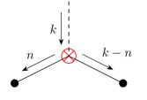
(a)

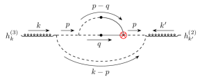
(b)

(c)

(d)

(e)

(f)

Figure 1: The two loop contributions from Eq. (14). The dashed and spring-like lines in the figure represent scalar and tensor perturbations, respectively. Figure (a) depicts the non-Gaussian vertex.

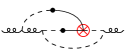
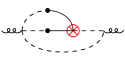
Figure 2: The two-loop diagrams correspond to the two-point functions: $\langle h^{\lambda,(3)}_{\mathbf{k},\phi\phi\phi}h^{\lambda^{\prime},(2)}_{\mathbf{k}^{\prime},\phi\phi}\rangle$, $\langle h^{\lambda,(3)}_{\mathbf{k},\phi h_{\phi\phi}}h^{\lambda^{\prime},(2)}_{\mathbf{k}^{\prime},\phi\phi}\rangle$, and $\langle h^{\lambda,(3)}_{\mathbf{k},\phi V_{\phi\phi}}h^{\lambda^{\prime},(2)}_{\mathbf{k}^{\prime},\phi\phi}\rangle$. The dashed lines, wavy lines and spring-like lines represent scalar, vector, and tensor perturbations, respectively.

The power spectra $\mathcal{P}^{(m,n)}_{k}(\eta)$ of the two-point function $\langle h^{\lambda,(m)}_{\mathbf{k}}(\eta)h^{\lambda^{\prime},(n)}_{\mathbf{k}^{\prime}}(\eta)\rangle$ are defined as

$$\langle h^{\lambda,(m)}_{\mathbf{k}}(\eta)h^{\lambda^{\prime},(n)}_{\mathbf{k}^{\prime}}(\eta)\rangle=\delta^{\lambda\lambda^{\prime}}\delta\left(\mathbf{k}+\mathbf{k}^{\prime}\right)\frac{2\pi^{2}}{k^{3}}\mathcal{P}^{(m,n)}_{k}(\eta)\ .$$ (15)

In the spherical coordinate system, we can obtain the explicit expression of the power spectrum that corresponds to Eq. (14)

$$\mathcal{P}^{(3,2)}_{\phi\psi_{\phi\phi},\phi\phi} =\frac{16f_{\mathrm{NL}}}{405\pi}\int_{0}^{\infty}{\rm d}v\int_{0}^{\infty}{\rm d}\bar{v}\int^{1+\bar{v}v}_{|1-\bar{v}v|}{\rm d}w\int^{1+v}_{|1-v|}{\rm d}u$$ (16)

$$\int_{\bar{u}_{-}}^{\bar{u}_{+}}{\rm d}\bar{u}\Big{\{}\frac{w}{u^{2}\bar{u}^{2}v\bar{v}^{2}\sqrt{Y(1-X^{2})}}~{}\Lambda^{lmrs}(\mathbf{k})p_{l}p_{m}$$

$$\times I^{(3)}_{\phi\psi_{\phi\phi}}\left(u,v,\bar{u},\bar{v},x\right)\sum_{a=1}^{n}\left(p^{\prime}_{r}p^{\prime}_{s}I^{(2)}_{\phi\phi}\left(u^{\prime},v^{\prime},x\right)\right)_{a}$$

$$P_{\zeta}(ku)P_{\zeta}(k\bar{u}v)P_{\zeta}(k\bar{v}v)\Big{\}}\ ,$$

where $P_{\zeta}$ is the primordial power spectrum which is defined as $\langle\zeta_{\mathbf{k}}\zeta_{\mathbf{k}^{\prime}}\rangle=\frac{2\pi^{2}}{k^{3}}\delta(\mathbf{k}+\mathbf{k}^{\prime})\mathcal{P}_{\zeta}(k)$. The subscripts $\phi\psi_{\phi\phi}$ and $\phi\phi$ on the left-hand side of the equation represent the source term of GW in the two-point correlation function. The summation of index $a$ in Eq. (16) represents the Wick’s expansions of the six-point function of $\zeta_{\mathbf{k}}$. The simplification of the integral in Eq. (16) is equivalent to that of the third order SIGW. The specific form and detailed derivation process of the integral can be found in Refs. Chang et al. (2022b); Zhou et al. (2022).

Note that there are four kinds of source terms for the third order SIGW in Eq. (8). The other three kinds of two-point correlation functions can also be investigated in the same way as Eq. (14). Fig. 2 shows the two-loop diagrams corresponding to all remaining two-point correlation functions.

Here, we consider the log-normal primordial power spectrum

$$\mathcal{P}_{\zeta}(k)=\frac{A_{\zeta}}{\sqrt{2\pi\sigma_{*}^{2}}}\exp\left(-\frac{\ln^{2}\left(k/k_{*}\right)}{2\sigma_{*}^{2}}\right)\ .$$ (17)

The total energy density spectrum of SIGW is given by

$$\Omega_{\mathrm{GW}}^{\mathrm{tot}} =\Omega_{\mathrm{GW}}^{(2,2)}+\Omega_{\mathrm{GW}}^{(2,3)}$$ (18)

$$=\frac{1}{6}\left(\frac{k}{a(\eta)H(\eta)}\right)^{2}\left(\frac{1}{4}\mathcal{P}^{(2,2)}_{h}+\frac{1}{6}\mathcal{P}^{(3,2)}_{h}\right)\ .$$

Taking into account the thermal history of the universe, we obtain the current total energy density spectrum $\Omega^{\mathrm{tot}}_{\mathrm{GW},0}$ Wang et al. (2019)

$$\Omega_{\mathrm{GW},0}^{\mathrm{tot}}=\Omega_{\mathrm{rad},0}\left(\frac{g_{*,\rho,\mathrm{e}}}{g_{*,\rho,0}}\right)\left(\frac{g_{*,s,0}}{g_{*,s,\mathrm{e}}}\right)^{4/3}\bar{\Omega}^{\mathrm{tot}}_{\mathrm{GW}}(\eta,k)\ .$$ (19)

After considering the contributions of seventeen new two-loop diagrams shown in Fig. 1 and Fig. 2, we present the current total energy density spectrum in Fig. 3. The power spectrum of SIGW originates from three contributions: the Gaussian $\langle h^{\lambda,(2)}_{\mathbf{k}}(\eta)h^{\lambda^{\prime},(2)}_{\mathbf{k}^{\prime}}(\eta)\rangle\sim A_{\zeta}^{2}$ , the non-Gaussian $\langle h^{\lambda,(2)}_{\mathbf{k}}(\eta)h^{\lambda^{\prime},(2)}_{\mathbf{k}^{\prime}}(\eta)\rangle\sim(f_{\mathrm{NL}})^{2}A_{\zeta}^{3}$, and the non-Gaussian $\langle h^{\lambda,(3)}_{\mathbf{k}}(\eta)h^{\lambda^{\prime},(2)}_{\mathbf{k}^{\prime}}(\eta)\rangle\sim f_{\mathrm{NL}}A_{\zeta}^{3}$. We use Ceffyl Lamb et al. (2023) package embedded in PTArcade Mitridate et al. (2023) to analyze the data from the first 14 frequency bins of NANOGrav 15-year data set. Since previous work has primarily considered only the contributions from the first two parts, as shown in Fig. 4, the blue curve of $f_{\mathrm{NL}}$ is symmetric about zero. After taking into account the contributions of the two-point correlation function $\langle h^{\lambda,(3)}_{\mathbf{k}}(\eta)h^{\lambda^{\prime},(2)}_{\mathbf{k}^{\prime}}(\eta)\rangle$, the green curve of $f_{\mathrm{NL}}$ is no longer symmetric, and the parameter interval $f_{\mathrm{NL}}\in[-5,-1]$ is significantly excluded. When $f_{\mathrm{NL}}\in[-5,-1]$, the contributions of the missing two-loop diagrams will critically suppress the total energy density spectrum (black curve in Fig. 3), which prevents the total energy density spectrum of SIGWs from fitting well with the observational data from NANOGrav 15-year in this parameter interval.

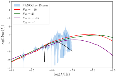
Figure 3: The total energy density spectra $\Omega_{\mathrm{GW},0}^{\mathrm{tot}}$ with $\sigma_{*}=1$ for different $f_{\mathrm{NL}}$. The parameters $\left(\log(A_{\zeta}),\log(k_{*})\right)$ for the red, green, purple, and black solid lines are $(-1.65,-7.3)$, $(-1.55,-7)$, $(-1,-7.5)$, and $(-1.1,-8.5)$, respectively. The energy density spectra derived from the free spectrum of NANOGrav 15-year data set are also shown here.

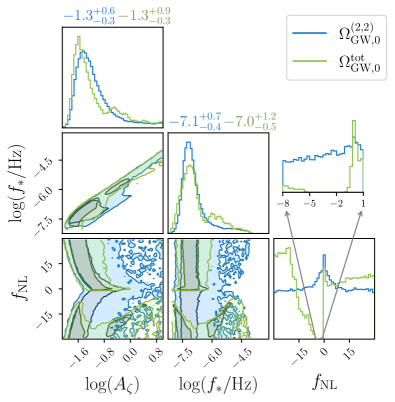
Figure 4: One and two-dimensional marginalized posteriors of three independent parameters, $\log(A_{\zeta})$, $\log(f_{*})$, and $f_{\mathrm{NL}}$. The priors are $\log(A_{\zeta})\in[-5,1]$, $\log(f_{*}/\mathrm{Hz})\in[-10,-3]$, and $f_{\mathrm{NL}}\in[-30,30]$. The previous one-loop and two-loop contributions are represented by the blue lines, and the green lines show the result after the addition of the new two-loop contributions.

For the PBH formation, a positive value of $f_{\mathrm{NL}}$ will augment the abundance of PBH for a given power spectrum of curvature perturbation. Conversely, a negative value of $f_{\mathrm{NL}}$ will reduce the abundance of PBH Young and Byrnes (2013). To avoid the overproduction of PBH, it is generally necessary to consider the case where $f_{\mathrm{NL}}<0$, since the abundance of PBHs cannot exceed that of dark matter Carr and Kuhnel (2020). When considering the constraints from PTA observations and the abundance of primordial black holes together, the possible range for $f_{\mathrm{NL}}$ is $f_{\mathrm{NL}}<-5$ or $-1\leq f_{\mathrm{NL}}<0$. Since the constraints of primordial non-Gaussianity on small scales ($\lesssim$1 Mpc) are significantly weaker than those on large scales Aghanim et al. (2020); Abdalla et al. (2022); Bringmann et al. (2012), $|f_{\mathrm{NL}}|$ could be substantially greater on small scales. It seems that the parameter interval $f_{\mathrm{NL}}<-5$ cannot be ruled out yet. However, to ensure the convergence of cosmological perturbations, $f_{\mathrm{NL}}$ and $A_{\zeta}$ must satisfy $(f_{\mathrm{NL}})^{2}A_{\zeta}<1$ and $A_{\zeta}<1$ in the non-Gaussian scenario. Fig. 4 shows that $\log(A_{\zeta})=(-1.3)^{+0.9}_{-0.3}$ with $1-\sigma$ credible region, implying that the absolute value of $f_{\mathrm{NL}}$ is less than $\sqrt{1/A_{\zeta}}\approx 4.47$. Consequently, even though the results with $f_{\mathrm{NL}}=-40$ in Fig. 3 can fit the NANOGrav 15-year data well, the region of the parameter space $f_{\mathrm{NL}}<-5$ might be ruled out by the convergence of perturbation expansion. Therefore, after taking into account the upper limit of the abundance of PBH and the convergence of the cosmological perturbation expansion, we find that the only possible range for $f_{\mathrm{NL}}$ might be $-1\leq f_{\mathrm{NL}}<0$ (purple line in Fig. 3).

Conclusion.—In this Letter, we systematically studied the seventeen missing two-loop diagrams proportional to $f_{\mathrm{NL}}A_{\zeta}^{3}$ that correspond to the two-point correlation function $\langle h^{\lambda,(3)}_{\mathbf{k}}h^{\lambda^{\prime},(2)}_{\mathbf{k}^{\prime}}\rangle$ in the case of local-type primordial non-Gaussianity. The missing two-loop contributions significantly impact the total energy density spectrum of the SIGW.

When combined with observations from the NANOGrav 15-year data, we found that if SIGW dominate the SGWB observed in PTA experiments, the parameter range for $f_{\mathrm{NL}}\in[-5,-1]$ will be entirely excluded. Furthermore, after taking into account the upper limit of the abundance of PBH and the convergence of the cosmological perturbation expansion, we conclude that the parameter spaces of $f_{\mathrm{NL}}\geq 0$ and $f_{\mathrm{NL}}<\sqrt{1/A_{\zeta}}\approx-4.47$ are ruled out, the only possible range for $f_{\mathrm{NL}}$ might be $-1\leq f_{\mathrm{NL}}<0$.