Self-similarity Prior Distillation for Unsupervised Remote Physiological Measurement

Abstract

Remote photoplethysmography (rPPG) is a non-invasive technique that aims to capture subtle variations in facial pixels caused by changes in blood volume resulting from cardiac activities. Most existing unsupervised methods for rPPG tasks focus on the contrastive learning between samples while neglecting the inherent self-similar prior in physiological signals. In this paper, we propose a Self-Similarity Prior Distillation (SSPD) framework for unsupervised rPPG estimation, which capitalizes on the intrinsic self-similarity of cardiac activities. Specifically, we first introduce a physical-prior embedded augmentation technique to mitigate the effect of various types of noise. Then, we tailor a self-similarity-aware network to extract more reliable self-similar physiological features. Finally, we develop a hierarchical self-distillation paradigm to assist the network in disentangling self-similar physiological patterns from facial videos. Comprehensive experiments demonstrate that the unsupervised SSPD framework achieves comparable or even superior performance compared to the state-of-the-art supervised methods. Meanwhile, SSPD maintains the lowest inference time and computation cost among end-to-end models. The source codes are available at https://github.com/LinXi1C/SSPD.

I Introduction

Cardiac activity is a fundamental physiological mechanism in the human body, and the assessment of physiological indicators, such as heart rate (HR), heart rate variability (HRV), and respiration frequency (RF) plays a critical role in maintaining physical and mental health. Traditionally, the acquisition of physiological measurements relies on contact medical instruments to obtain electrocardiogram (ECG) or photoplethysmography (PPG) signals, which may induce discomfort to users. Furthermore, in certain scenarios, such as driving [1] or telemonitoring [2], contact devices are no longer convenient. The remote photoplethysmography (rPPG) method, which captures subtle facial pixel changes caused by blood volume variations, has emerged as a promising alternative due to its non-invasive and low-cost characteristics.

In recent years, rPPG methods [3, 4, 5] have exhibited competitive performance for physiological measurement under the prevalence of deep learning. The primary challenges in rPPG tasks are related to the feebleness of the facial physiological signals and the strong noise in video recordings, including head movements [6], illumination changes [7], and video artifacts [8]. To tackle these issues, researchers have elaborated various rPPG datasets [9, 10, 11] and proposed effective supervised learning models [12, 13, 14] for rPPG estimation. The acquisition of high-quality labels requires high-precision contact instruments, such as electrodes for ECG [11] and photoelectric sensors for BVP [9, 10, 15, 16]. Furthermore, the signals must be recorded for a long period with contact, which can be a labor-intensive and time-consuming process [17]. Fortunately, unsupervised methods are a promising alternative as they can free the model from the dependence on supervision signals.

Unsupervised methods in the rPPG field can be categorized into two branches: signal-based and learning-based methods. Traditional signal-based methods [18, 19, 20, 21] tend to design models manually according to some specific assumptions (e.g., skin reflection model). These assumptions are mere simplifications of real scenarios, thus making signal-based methods vulnerable to various environment noise. On the other hand, most existing learning-based methods tend to use contrastive learning to extract physiological features, focusing on how to design positive and negative sample pairs, which can be generated from the same clip with temporal disordering [22] or frequency resampling [23, 24], or from different clips with augmentation [25, 26] or frequency resampling [27]. The contrastive loss can be performed on the latent representations followed by fine-tuning [22, 25, 26], directly on the output rPPG [23, 24], or on the power spectrum density (PSD) derived from the rPPG [5, 27].

However, these methods ignore the crucial self-similar physiological prior inherent in cardiac activities. Self-similarity indicates consistency in a dynamic system where a pattern or event appears similar to itself across different scales or intervals. This natural phenomenon is illustrated by the fractal patterns in the Mandelbrot set [28]. For the rPPG task, self-similarity can be observed from recurring events in every cardiac cycle, such as ventricular contraction and relaxation, which result in self-similar patterns at regular intervals in the facial video. As an intra-sample prior, self-similarity has finer granularity compared to the inter-sample prior used in contrastive learning [5, 23, 25]. Specifically, contrastive learning emphasizes the distance metric between positive and negative sample pairs, while self-similarity prior distillation focuses on effectively capturing the physiological features within individual samples.

In this paper, we propose a self-similarity prior distillation framework for unsupervised remote physiological measurement, which capitalizes on the intrinsic self-similarity of cardiac activities. Specifically, we first develop a physical-prior embedded augmentation technique, consisting of Local-Global Augmentation (LGA) and Masked Difference Modeling (MDM) against noise from both spatial and temporal aspects. Next, we tailor a self-similarity-aware network that comprises a backbone, a predictor module, and a Separable Self-Similarity Model ($S^{3}M$). The predictor module is responsible for estimating the rPPG signal, while the $S^{3}M$ generates a temporal similarity pyramid consisting of self-similarity maps at multiple time scales, facilitating self-similarity-aware learning. Furthermore, $S^{3}M$ serves as a training auxiliary to boost the performance without incurring extra computational expenses during inference. Finally, we design a hierarchical self-distillation paradigm to help the network disentangle self-similarity physiological patterns from facial videos. The proposed hierarchical self-distillation involves RPPG Prediction Distillation (RPD) and Temporal Similarity Pyramid Distillation (TSPD) to distill knowledge in both signal space and latent space.

In summary, the contributions of this work are as follows:

(1) We propose a Self-Similarity Prior Distillation (SSPD) framework for unsupervised remote physiological measurement, which exploits the inherent self-similarity of cardiac activities via a hierarchical self-distillation strategy.

(2) We develop two physical-prior embedded augmentation strategies to mitigate the effect of various types of noise from both spatial and temporal aspects.

(3) We devise a Separable Self-Similarity Model ($S^{3}M$) to enable self-similarity-aware learning, forcing the network to learn multi-scale and long-distance physiological features better, without incurring any extra computing expenses in the inference stage.

(4) We conduct extensive evaluations on four commonly used open-access benchmarks (PURE [15], UBFC-rPPG [16], VIPL-HR [9], and MR-NIRP [10]). The substantial experimental results demonstrate that SSPD outperforms the state-of-the-art unsupervised methods significantly.

II Related Works

II-A Self-supervised Learning

Unsupervised/self-supervised learning aims to let model learn a good representation from input data without human-annotated labels, guided by solving the pretext task. In recent years, self-supervised learning has achieved great success in natural language processing [29, 30] and computer vision tasks [31, 32, 33]. Self-supervised methods presented to date can be broadly categorized into three paradigms: contrastive learning [31, 34, 35, 36], masked modeling [29, 32, 37, 38] and self-distillation [33, 39]. The fundamental principle of contrastive learning is to attract positive sample pairs while repulsing negative pairs [40]. However, BYOL [41] demonstrates that contrastive learning can still be effective without the use of negative samples. Masked modeling performs a pretext task of predicting the masked content based on the remaining uncorrupted input. In other words, the supervision signal for masked modeling is derived solely from the input samples themselves. Self-distillation is a type of knowledge distillation [42, 43] in which the model learns from itself. Specifically, the teacher and student models share an identical structure, and the output of different layers can serve as supervision signals, which are also known as distilled knowledge. To obtain better knowledge, different instance discrimination [44] strategies have been proposed to generate diverse input views. Caron et al. [33] presented a self-distillation model DINO, leveraging the multi-crop [45] strategy to promote local-to-global correspondences. Furthermore, Zhou et al. [39] proposed the iBOT model, which utilizes masked image modeling inspired by BERT [29]. Unlike the conventional self-supervised learning paradigm of unsupervised pretraining followed by supervised fine-tuning, our approach adopts unsupervised online fine-tuning from self-similarity knowledge to directly generate the downstream rPPG signal. Additionally, the rPPG signal also serves as another knowledge for self-distillation.

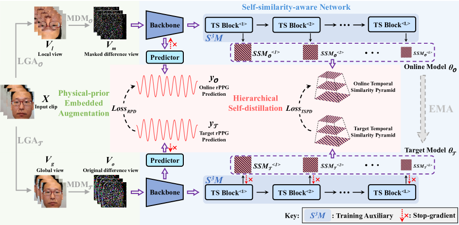
Figure 1: The architecture of our SSPD framework for unsupervised remote physiological measurement. This framework first incorporates Local-Global Augmentation (LGA) and Masked Difference Modeling (MDM) to generate two input views. Then, the tailored self-similarity-aware network consists of a backbone, a predictor module, and a Separable Self-Similarity Model ($S^{3}M$). Each Temporal Similarity (TS) block in $S^{3}M$ exploits self-similar representations at a specific time scale, forming the temporal similarity pyramid $\{SSM^{<1>},SSM^{<2>},...,SSM^{<L>}\}$, and the $S^{3}M$ is used exclusively for training. Finally, the proposed hierarchical self-distillation paradigm comprises RPPG Prediction Distillation (RPD) and Temporal Similarity Pyramid Distillation (TSPD), which aim to distill knowledge in both signal space and latent space.

II-B Remote Physiological Measurement

Traditional methods take the approach of decomposing the temporal sequence signal to expose the rPPG signal of genuine interest. Therefore, signal disentanglement methods (e.g., ICA [18], PCA [46, 47]) and skin reflection modeling methods (e.g., CHROM [19], POS [21]) are proposed. However, deep learning methods take the path of estimating the rPPG and noise distribution from the input video and thus have better robustness. In supervised rPPG estimation, Chen et al. [6] proposed the first end-to-end model, namely DeepPhys. This model takes the original frame and frame difference as inputs to the appearance and motion models, respectively, fusing them through an attention mechanism. Building upon this, the two-stream models [12, 48, 49] have been demonstrated to be effective for rPPG estimation. Meanwhile, spatial-temporal representation learning [8, 13, 50, 51] has emerged as a promising alternative, which typically employs a 3D convolutional neural network (CNN) or vision transformer [52] as the backbone. Additionally, an effective preprocessing paradigm called STMaps [3, 7, 53] has been designed. STMaps involve the selection of multiple regions of interest (ROIs) from facial video, which allows the network to focus more on rPPG features and reduce the impact of noise.

However, annotating large-scale datasets in deep learning [54, 55], particularly in physiological measurement, has always been a labor-intensive and time-consuming process. The acquisition of long-period physiological signals as ground truth is expensive and challenging, which has led to the emergence of self-supervised learning as a promising alternative for rPPG estimation [5, 23, 25]. Gideon and Stent [23] leveraged two primary prior knowledge constraints: HR ranges between 40 to 250 bpm and HR is stable over short time intervals. They adopted spectrum perturbation to generate positive-anchor-negative triplet samples for contrastive learning. Furthermore, Sun and Li [5] proposed the Contrast-Phys model, which utilized spatial and temporal inter-sample similarity as finer-grain prior knowledge of rPPG. Additionally, Park et al. [26] presented a contrastive vision transformer framework for the joint modeling of RGB and near-infrared (NIR) videos. Most existing self-supervised methods focus on constructing positive and negative samples but overlook the inherent self-similarity property of physiological signals. In our SSPD framework, we identify the self-similar patterns between local and global views, as well as between the original and masked views, without requiring negative samples.

III Method

III-A Overview

In this section, we present a detailed explanation of the proposed Self-Similarity Prior Distillation (SSPD) framework for unsupervised remote physiological measurement. As shown in Fig. 1, the overall pipeline consists of three main stages. First, we apply physical-prior embedded augmentation to generate two distinct input views. Second, we devise a self-similarity-aware network composed of a backbone and predictor module for rPPG estimation and a Separable Self-Similarity Model ($S^{3}M$) to facilitate self-similarity-aware learning. Third, we develop a hierarchical self-distillation paradigm to disentangle self-similar physiological patterns from facial videos.

III-B Physical-prior Embedded Augmentation

In the rPPG task, noise sources can be broadly categorized into head movements, illumination changes, and video artifacts. To capture shift-invariant features in the space domain, we introduce the Local-Global Augmentation (LGA) method to enhance local-global responses. Furthermore, to enhance the robustness of the model to time-invariant noise present in illumination changes and video artifacts, such as camera noise and quantization error [6], we employ frame difference mapping to help the model focus more on motion-related information than appearance-based features. Moreover, to reduce the impact of time-variant motion noise within the frame difference map, we introduce random masking, which also serves as a nontrivial pretext task [32] for self-similarity-aware learning. Together, the combination of frame difference mapping and random masking constitutes Masked Difference Modeling (MDM).

III-B1 Video Preprocessing

Initially, the face region is detected and cropped from the original video clip with a length of $T+1$ using the Dlib library [56]. The bounding box is only generated based on the first frame and maintained in the subsequent frames of the clip. Next, the bounding box is resized to 151$\times$151 for physical-prior embedded augmentation, denoted as $X\in\mathbb{R}^{(T+1)\times 3\times 151\times 151}$.

III-B2 Local-global Augmentation

We employ Local-Global Augmentation (LGA) for spatial augmentation. The LGA strategy aims to enable the model to capture shift-invariant features by enhancing local-global responses. This makes the model more robust to spatial variations in the facial area, such as the shaking of the facial bounding box or changes in the distance between the head and the camera. Specifically, we generate the local view $V_{l}\in\mathbb{R}^{(T+1)\times 3\times 128\times 128}$ and the global view $V_{g}\in\mathbb{R}^{(T+1)\times 3\times 128\times 128}$ from the same input clip $X$. The local view $V_{l}$ is produced by random cropping, horizontal and vertical flipping with the shape of 128$\times$128, while the global view $V_{g}$ is obtained by resizing, randomly horizontal and vertical flipping with the same shape. Noteworthy, the augmentations utilized in LGA are solely applied to the spatial dimension, indicating that each frame in the video clip undergoes identical transformations.

III-B3 Masked Difference Modeling

Building upon the aforementioned LGA strategy, we elaborate the Masked Difference Modeling (MDM) for temporal augmentation, which leverages the self-similarity prior of physiological signals. The procedure of MDM can be described as follows:

$$V_{m} =m\odot(\Delta_{t}V_{l,t})$$ (1)

$$V_{o} =\Delta_{t}V_{g,t}$$

specifically, we calculate the first forward difference [6] between two consecutive frames of $V_{l}$, where $\Delta_{t}V_{l,t}=V_{l,t+1}-V_{l,t}$. Then we apply a binary mask $m\in\{0,1\}^{T\times 3\times 128\times 128}$ to $\Delta_{t}V_{l,t}$, where each element of $m$ is independently sampled from Bernoulli distribution with a probability of $p$. The resulting masked difference view $V_{m}$ is the element-wise multiplication of the mask and the difference noted as $\odot$. Besides, the original difference view $V_{o}$ is solely generated through frame difference without masking.

The reasons why we apply a mask to the frame difference are as follows: (a) The mask itself can be viewed as a nontrivial pretext task. The presence of self-similar patterns in physiological signals enables the reconstruction of features affected by the mask from other frames at different timestamps, which promotes the model’s ability to capture temporal self-similar representations. (b) Frame difference typically contains a considerable amount of noise induced by motions irrelevant to rPPG (such as head movements and illumination changes). The mask serves as a matrix sparsity operation, which functions as a form of pre-denoising. (c) The mask ratio is always dynamic since the prior mean of the frame difference is 0, while a dynamic data augmentation technique can further improve the robustness of the model.

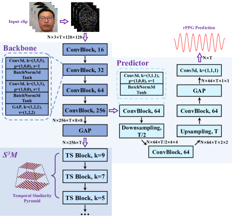
Figure 2: The architecture of the self-similarity-aware network. Each “ConvBlock” comprises two convolution layers, with “GAP” representing global average pooling. “Downsampling” refers to a reduction of half in the time domain. The dimensions are presented as N$\times$C$\times$T$\times$H$\times$W, where N and C indicate the number of samples and channels, respectively.

III-C Self-similarity-aware Network

Self-similarity is a crucial physiological phenomenon that describes the recurring events that occur in every cardiac cycle associated with heartbeat generation. Such physiological mechanisms generate regular patterns that appear at different intervals in facial videos. To capture self-similar representations synchronized with heartbeat rhythms, we present a self-similarity-aware network consisting of a backbone for spatial-temporal feature extraction, a predictor module for downstream fine-tuning, and a Separable Self-Similarity Model ($S^{3}M$) for enabling self-similarity-aware learning.

III-C1 Backbone & Predictor Module

The backbone in the SSPD framework consists of four spatial-temporal convolutional blocks, which are designed to produce preliminary spatial-temporal feature maps. To fine-tune for downstream tasks, such as rPPG estimation, a predictor module is attached before the last global average pooling (GAP) layer in the backbone, and the detailed structure of the backbone and predictor module are presented in Fig. 2. During the training and inference stages, the backbone of the online model $\theta_{\mathcal{O}}$ and target model $\theta_{\mathcal{T}}$ receive the masked difference view $V_{m}$ and the original difference view $V_{o}$ as input, respectively. The outputs of the backbones are represented as $S_{\mathcal{O}}\in\mathbb{R}^{T\times C}$ and $S_{\mathcal{T}}\in\mathbb{R}^{T\times C}$ , and the predicted rPPG output from the predictor modules can be expressed as $y_{\mathcal{O}}\in\mathbb{R}^{T}$ and $y_{\mathcal{T}}\in\mathbb{R}^{T}$, respectively. Noteworthy, the learning objectives designed for the backbone and the predictor module are not completely congruent. The backbone is biased to temporal self-similar representations, which are further enhanced and backpropagated from subsequent $S^{3}M$ during training. We further fine-tune these representations using the predictor module to obtain rPPG estimation, which focuses more on downstream tasks. Thus, to prevent gradient conflict, we apply a stop-gradient operation between the backbone and predictor module depicted in Fig. 1.

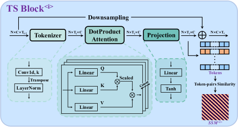
Figure 3: The architecture of the Temporal Similarity (TS) block. Firstly, the input sequences are projected into token embeddings at a specific time scale. Next, the multi-head dot-product attention improves the global context information, followed by a linear projection. We derive the self-similarity map ($SSM$) which forms a layer in the temporal similarity pyramid from the token embeddings. We add a residual connection from the input sequence to the output tokens and perform downsampling for dimension alignment.

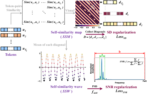
Figure 4: The derivation of self-similarity map, self-similarity wave, and complementary regularizations. The self-similarity map is obtained by computing the cosine similarity between every pair of tokens. Subsequently, we calculate the mean value of each diagonal, yielding the self-similarity wave. The complementary regularizations comprise the Standard Deviation (SD) regularization and Signal-to-Noise Ratio (SNR) regularization. SD regularization constrains the standard deviation of each diagonal from the self-similarity map, while SNR regularization constrains the SNR of the self-similarity wave.

III-C2 Separable Self-similarity Model

To enable self-similarity-aware learning, we elaborate a Separable Self-Similarity Model ($S^{3}M$) that forces the network to learn multi-scale and long-distance physiological features better. Importantly, this model is separable and serves as a training auxiliary without incurring any extra computing expenses in the inference stage. Specifically, the proposed $S^{3}M$ is composed of cascaded Temporal Similarity (TS) blocks that transform the input sequences (i.e., $S_{\mathcal{O}}$, $S_{\mathcal{T}}$) into self-similarity maps, which are subsequently incorporated into the temporal similarity pyramid. Each TS block within the model corresponds to a specific temporal scale, enabling the model to focus on multi-scale self-similar features that are synchronized with heartbeat events. In particular, as illustrated in Fig. 3, we initially tokenize the input sequence $S^{<i>}\in\mathbb{R}^{T_{i-1}\times C}$ into token embeddings $E^{<i>}=\{e_{1}^{<i>},e_{2}^{<i>},...,e_{T_{i}}^{<i>}\}$, where $e_{t}^{<i>}\in\mathbb{R}^{C}$ and $i$ denotes the i-th level TS block. Subsequently, we apply the multi-head dot-product attention [57] to enhance the global contextual relationships among the tokens, rather than utilizing self-attention directly. This is because the attention scores in self-attention are constrained within the range of (0, 1) due to the Softmax(·) normalization. To better facilitate the learning of long-distance physiological features, we expand the attention scores to the ($-\infty$, $+\infty$) range to maintain symmetry between positive and negative values. Specifically, we firstly project the input tokens $E^{<i>}$ to $K^{<i>}\in\mathbb{R}^{T_{i}\times C}$, $Q^{<i>}\in\mathbb{R}^{T_{i}\times C}$, $V^{<i>}\in\mathbb{R}^{T_{i}\times C}$, respectively. Then, we calculate the attention output as shown below:

$$A^{<i>} =\frac{Q^{<i>}{K^{<i>}}^{T}}{C}V^{<i>}$$ (2)

here, $T$ stands for matrix transpose. Noteworthy, we also leverage multi-head joint modeling, which is the same as [58]. After that, we adopt another linear projection layer with parameters $W^{<i>}\in\mathbb{R}^{C\times C}$ to $A^{<i>}$, resulting in $U^{<i>}=\{u_{1}^{<i>},u_{2}^{<i>},...,u_{T_{i}}^{<i>}\}$, where $u_{t}^{<i>}\in\mathbb{R}^{C}$. Next, we produce the self-similarity map as the final output of the TS block, as shown in Fig. 3. The self-similarity map $SSM^{<i>}\in\mathbb{R}^{T_{i}\times T_{i}}$ is formed by computing the similarity between each pair of tokens, denoted as $SSM^{<i>}=\{Sim(u_{j}^{<i>},u_{k}^{<i>})|j,k\in\left[1,T_{i}\right]\}$, where the Sim(·) represents cosine similarity as follows:

$$Sim(u_{j}^{<i>},u_{k}^{<i>}) =\frac{u_{j}^{<i>}\cdot u_{k}^{<i>}}{\|u_{j}^{<i>}\|_{2}\cdot\|u_{k}^{<i>}\|_{2}}$$ (3)

Furthermore, we obtain the self-similarity wave $SSW^{<i>}\in\mathbb{R}^{T_{i}}$ by calculating the mean value of each diagonal located in the upper triangle of the $SSM^{<i>}$ matrix, as illustrated in Fig. 4. Specifically, we first retrieve the diagonals on the upper triangle of $SSM^{<i>}$ to generate the diagonal set $D^{<i>}=\{d_{1}^{<i>},d_{2}^{<i>},...,d_{T_{i}}^{<i>}\}$, where $d_{t}^{<i>}=\{Sim(u_{j}^{<i>},u_{k}^{<i>})|k-j=t-1\}$, $t\in\left[1,T_{i}\right]$. Subsequently, we form the self-similarity wave:

$$SSW^{<i>}=\{\frac{1}{t}\sum_{n=1}^{t}d_{t,n}^{<i>}|d_{t}^{<i>}\in D^{<i>}\}$$ (4)

In addition, we add a residual connection [59] from the input sequence $S^{<i>}$ to the output token embeddings $U^{<i>}$, and we utilize adaptive average pooling to maintain the alignment of the temporal dimension, which is illustrated below:

$$S^{<i+1>} =POOL_{T_{i-1}\rightarrow T_{i}}(S^{<i>})+U^{<i>}$$ (5)

The residual connection allows us to increase the number of TS blocks in $S^{3}M$ without significant degradation, facilitating the capture of self-similar representations under different temporal scales. Finally, we integrate the output of the TS blocks at multiple time scales, forming the temporal similarity pyramid $\{SSM^{<1>},SSM^{<2>},...,SSM^{<L>}\}$, along with the $\{SSW^{<1>},SSW^{<2>},...,SSW^{<L>}\}$, where $L$ denotes the total number of blocks, i.e., the number of pyramid layers.

The $S^{3}M$ contributes significantly to extracting more reliable physiological features through self-similarity-aware learning, we further make it separable to guarantee that there are no extra computational expenses in the inference stage due to the incorporation of $S^{3}M$. To this end, we devise two distinct feature flow paths for training and inference, as depicted in Fig. 1. During the training stage, feature maps are propagated through all modules in the SSPD framework, resulting in the rPPG prediction $y_{\mathcal{O}}$, $y_{\mathcal{T}}$, and the temporal similarity pyramid $\{SSM_{\mathcal{O}}^{<1>},SSM_{\mathcal{O}}^{<2>},...,SSM_{\mathcal{O}}^{<L>}\}$, $\{SSM_{\mathcal{T}}^{<1>},SSM_{\mathcal{T}}^{<2>},...,SSM_{\mathcal{T}}^{<L>}\}$ for self-distillation. While in the inference stage, all TS blocks in $S^{3}M$ are discarded, and the rPPG estimation is obtained solely from the backbone and subsequent predictor module. Consequently, by using the $S^{3}M$, our framework can facilitate better learning of multi-scale and long-distance physiological features without increasing the computational cost during inference.

Input:

$\theta_{\mathcal{O}}$, $\theta_{\mathcal{T}}$;                   # online and target models

$x$;                          # input clip

$\rho$;                          # momentum rate

LGA;                      # local-global augmentation

MDM;                    # masked difference modeling

$\mathcal{L}_{Pearson}$;                # negative Pearson loss

$\mathcal{L}_{SD}$, $\mathcal{L}_{SNR}$;            # SD and SNR regularizations

$\theta_{\mathcal{O}}$.params = $\theta_{\mathcal{T}}$.params

for $x$ in loader do

       $v_{l}$, $v_{g}$ = LGA_O($x$), LGA_T($x$)

       $v_{m}$, $v_{o}$ = MDM_O($v_{l}$), MDM_T($v_{g}$)

       # rPPG, temporal similarity pyramid

       $y_{\mathcal{O}}$, $SSM_{\mathcal{O}}$ = $\theta_{\mathcal{O}}$($v_{m}$)

       $y_{\mathcal{T}}$, $SSM_{\mathcal{T}}$ = $\theta_{\mathcal{T}}$($v_{o}$)

      

      $\mathcal{L}_{SSPD}$ = D($y_{\mathcal{O}}$, $SSM_{\mathcal{O}}$, $y_{\mathcal{T}}$, $SSM_{\mathcal{T}}$)

                     + $\alpha\cdot\mathcal{L}_{SD}$($SSM_{\mathcal{O}}$) + $\beta\cdot\mathcal{L}_{SNR}$($SSM_{\mathcal{O}}$)

      $\mathcal{L}_{SSPD}$.backward()

       update($\theta_{\mathcal{O}}$)

       $\theta_{\mathcal{T}}$.params = $\rho$·$\theta_{\mathcal{T}}$.params + (1$-\rho$)·$\theta_{\mathcal{O}}$.params

end for

def D($r_{1}$, $p_{1}$, $r_{2}$, $p_{2}$):

       $r_{2}$, $p_{2}$ = $r_{2}$.detach(), $p_{2}$.detach()

       # fourier transform

       $psd_{1}$, $psd_{2}$ = FFT($r_{1}$), FFT($r_{2}$)       

       # mean of each diagonal

       $w_{1}$, $w_{2}$ = Diagonals($p_{1}$), Diagonals($p_{2}$)   

       $\mathcal{L}_{Distill}$ = $\mathcal{L}_{Pearson}$($r_{1}$, $r_{2}$) + $\mathcal{L}_{MSE}$($psd_{1}$, $psd_{2}$) +

                    $\mathcal{L}_{MSE}$($p_{1}$, $p_{2}$) + $\mathcal{L}_{MSE}$($w_{1}$, $w_{2}$)

       return $\mathcal{L}_{Distill}$

Algorithm 1 SSPD PyTorch-like Pseudocode

III-D Hierarchical Self-distillation

As presented in Sec. III-B, we utilize LGA and MDM to augment two distinct input views from both spatial and temporal aspects. To facilitate self-similarity-aware learning in the time domain, we enable the online model to recover the masked view $V_{m}$ to its corresponding target model output in the self-similar latent space, with the temporal similarity pyramid from the target model serving as the label. Additionally, since the local and global views have different spatial scales, we aim to discover the shared temporal self-similarity from both views as spatial-invariant representations. Accordingly, we tailor the hierarchical self-distillation paradigm in our SSPD framework, which not only aligns the rPPG signal of interest but also distills the underlying temporal self-similar representations. Specifically, the hierarchical distilled knowledge comprises two parts: RPPG Prediction Distillation (RPD) and Temporal Similarity Pyramid Distillation (TSPD), which exploit the knowledge in signal space and latent space, respectively. Additionally, we devise two complementary regularizations to boost the performance of distillation based on physical priors. To prevent model collapse [41], we implement a stop-gradient operation on the target model, and we use the exponential moving average (EMA) [31] to update its parameters from the online model.

III-D1 RPPG Prediction Distillation

We propose the RPPG Prediction Distillation (RPD), which directly distills the predicted rPPG signal (i.e., $y_{\mathcal{O}}$, $y_{\mathcal{T}}$) as the signal space knowledge. We calculate the normalized PSD noted as $f_{y_{\mathcal{O}}}$, $f_{y_{\mathcal{T}}}$, and the RPD loss can be described as follows:

$$\mathcal{L}_{RPD} =\mathcal{L}_{Pearson}(y_{\mathcal{O}},y_{\mathcal{T}})+\frac{1}{N}\sum_{i=1}^{N}\left\lVert f_{y_{\mathcal{O}}}^{i}-f_{y_{\mathcal{T}}}^{i}\right\rVert^{2}_{2}$$ (6)

here $\mathcal{L}_{Pearson}(\cdot)$ means negative Pearson loss [13], and N is the number of samples.

III-D2 Temporal Similarity Pyramid Distillation

Compared to the aforementioned RPD, Temporal Similarity Pyramid Distillation (TSPD) aligns the output features from the online and target models in self-similarity latent space, serving as the latent space knowledge. The temporal similarity pyramids (i.e., $\{SSM_{\mathcal{O}}^{<1>},SSM_{\mathcal{O}}^{<2>},...,SSM_{\mathcal{O}}^{<L>}\}$, $\{SSM_{\mathcal{T}}^{<1>},SSM_{\mathcal{T}}^{<2>},...,SSM_{\mathcal{T}}^{<L>}\}$) indicate the temporal self-similar representations induced by heartbeat events, which are inherent characteristics shared by different input views. We measure the distance between each layer of the temporal similarity pyramid, and the TSPD loss can be defined as follows:

$$\mathcal{L}_{TSPD}= \frac{1}{N}\sum_{i=1}^{N}\sum_{j=1}^{L}(\left\lVert{SSM_{\mathcal{O}}^{<j>}}^{i}-{SSM_{\mathcal{T}}^{<j>}}^{i}\right\rVert^{2}_{2}$$ (7)

$$+\left\lVert{SSW_{\mathcal{O}}^{<j>}}^{i}-{SSW_{\mathcal{T}}^{<j>}}^{i}\right\rVert^{2}_{2})$$

Finally, our hierarchical self-distillation loss is the sum of RPD loss and TSPD loss:

$$\mathcal{L}_{Distill}=\mathcal{L}_{RPD}+\mathcal{L}_{TSPD}$$ (8)

III-D3 Complementary Regularizations

To boost the performance of self-similarity-aware learning, we design two complementary regularizations for the online model based on physical priors. As depicted in Fig. 4, we first propose the Standard Deviation (SD) regularization to assist the model in exploiting the quasi-period nature of the rPPG signal, which exhibits similar patterns at regular intervals. We retrieve the diagonals on the upper triangle of $SSM^{<i>}$ to form the diagonal set $D^{<i>}=\{d_{1}^{<i>},d_{2}^{<i>},...,d_{T_{i}}^{<i>}\}$, where $d_{t}^{<i>}\in\mathbb{R}^{t}$. Then we compute the SD regularization loss as follows:

$$\mathcal{L}_{SD}=\frac{1}{N}\frac{1}{L}\frac{1}{T_{j}}\sum_{i=1}^{N}\sum_{j=1}^{L}\sum_{k=1}^{T_{j}}SD(\varepsilon k\cdot{d_{k}^{<j>}}^{i})$$ (9)

where the $SD(\cdot)$ means standard deviation [60], and we use $\varepsilon$ to modulate the range of the SD output. Experimentally, $\varepsilon$ is 0.05 by default.

However, as the rPPG signal is not completely periodic [61], excessive emphasis on SD regularization can lead to a dominant direct composition (DC) component in the self-similarity map, resulting in a homogeneous map with elements nearing 1. Thus, we devise the Signal-to-Noise Ratio (SNR) regularization to avoid the DC collapse caused by SD regularization, as shown in Fig. 4. We calculate the normalized PSD of the $SSW^{<i>}$, noted as $f_{SSW^{<i>}}$, and we adjust the definition of SNR as proposed in [62]:

TABLE I: Intra-dataset and cross-dataset HR estimation results compared to the state-of-the-art methods. The best results are highlighted in bold. The notation “-L3” indicates that the temporal similarity pyramid consists of three layers, while “$\dagger$” denotes the model is trained on the VIPL-HR dataset and evaluated on other datasets.

		UBFC-rPPG			PURE			MR-NIRP
Method Types	Methods	MAE$\downarrow$	RMSE$\downarrow$	R$\uparrow$	MAE$\downarrow$	RMSE$\downarrow$	R$\uparrow$	MAE$\downarrow$	RMSE$\downarrow$	R$\uparrow$
	GREEN [20]	8.33	10.88	0.48	5.83	10.64	0.59	-	-	-
	POS [21]	7.80	11.44	0.62	2.99	4.79	0.94	-	-	-
Traditional	CHROM [19]	6.69	8.82	0.82	4.17	6.26	0.92	-	-	-
	ICA [18]	5.63	8.53	0.71	2.59	4.23	0.94	-	-	-
	CAN [12]	-	-	-	1.27	3.06	0.97	7.78	16.8	-0.03
	HR-CNN [63]	-	-	-	1.84	2.37	0.98	-	-	-
	SynRhythm [14]	5.59	6.82	0.72	-	-	-	-	-	-
	PhysNet [13]	-	-	-	2.1	2.6	0.99	3.07	7.55	0.655
	PulseGAN [64]	1.19	2.10	0.98	-	-	-	-	-	-
	Dual-GAN [3]	0.44	0.67	0.99	0.82	1.31	0.99	-	-	-
Supervised	Nowara2021 [65]	-	-	-	-	-	-	2.34	4.46	0.85
	RemotePPG [23]	1.85	4.28	0.93	2.3	2.9	0.99	4.75	9.14	0.61
	Contrast-Phys [5]	0.64	1.00	0.99	1.00	1.40	0.99	2.68	4.77	0.85
Unsupervised	SSPD-L3	0.50	0.71	0.99	0.53	1.16	0.99	2.65	3.66	0.94
	cross-dataset evaluations
	RemotePPG† [23]	4.67	8.75	0.72	2.22	3.82	0.96	7.93	11.01	0.05
	Contrast-Phys† [5]	1.90	3.30	0.95	3.07	4.85	0.94	5.73	9.18	0.18
	SSPD-L3†	1.08	1.81	0.99	1.24	1.77	0.99	3.52	6.21	0.73

TABLE II: HR estimation results of 5-fold cross-validation on the VIPL-HR dataset. The best results are highlighted in bold. The ^◆ denotes that the evaluation protocol aligns with the [26], except that SSPD does not require any labels for fine-tuning.

Method Types	Methods	SD$\downarrow$	MAE$\downarrow$	RMSE$\downarrow$	R$\uparrow$
Traditional	GREEN [20]	8.93	11.34	14.41	0.16
	POS [21]	11.57	15.89	19.63	0.52
	CHROM [19]	11.39	13.88	17.93	0.45
	ICA [18]	9.75	10.68	14.44	0.17
Supervised	PhysNet [13]	14.9	10.8	14.8	0.20
	DeepPhys [6]	13.6	11.0	13.8	0.11
	RhythmNet [7]	8.11	5.30	8.14	0.76
	PhysFormer [4]	7.74	4.97	7.79	0.78
	Dual-GAN [3]	7.63	4.93	7.68	0.81
Unsupervised	ViViT◆ [26]	14.15	10.75	14.20	-0.039
	SSPD-L3-160◆	9.69	8.37	12.79	0.54
	RemotePPG [23]	10.85	8.50	13.76	0.31
	Contrast-Phys [5]	8.04	8.80	11.92	0.24
	SSPD-L3	7.42	6.04	9.56	0.59

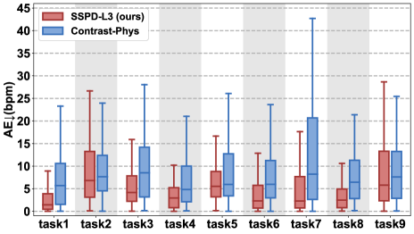
Figure 5: Absolute error (AE) across different scenarios for all subjects in the VIPL-HR dataset. AE is measured as the difference between the estimated HR and the ground truth HR. The 9 scenarios in the dataset are represented by task1-task9, which correspond to stable, motion, talking, bright, dark, long distance, exercise, phone stable, and phone motion scenarios, respectively.

$$SNR(f)=\frac{\sum_{a}f}{\sum_{b}f-\sum_{a}f}$$ (10)

In our work, $a$ represents the frequency range from 0.5 Hz to 3 Hz, which corresponds to the typical range of heart rate frequencies [23]. $b$ includes the entire frequency band, ranging from 0 Hz to $F_{s}/2$ Hz, where $F_{s}$ is the sampling rate. Given these definitions, we propose the SNR regularization as follows:

$$\mathcal{L}_{SNR}=\frac{1}{N}\frac{1}{L}\sum_{i=1}^{N}\sum_{j=1}^{L}\frac{1}{SNR({f_{SSW^{<j>}}}^{i})}$$ (11)

Nevertheless, this overstrict frequency constraint has the effect of diminishing subtle waveform dynamics, such as diastolic peaks [49]. In conclusion, the SD regularization and the SNR regularization are complementary w.r.t. the prior knowledge of rPPG and converge to an optimal point through dynamic equilibrium.

To sum up, the total loss of the SSPD framework can be built as follows:

$$\mathcal{L}_{SSPD}=\mathcal{L}_{Distill}+\alpha\cdot\mathcal{L}_{SD}+\beta\cdot\mathcal{L}_{SNR}$$ (12)

where hyperparameters $\alpha$, $\beta$ equal to 0.8, 0.6, respectively. During training, we only optimize the online model by back-propagation, while the parameters of the target model are directly updated using EMA:

$$\theta_{\mathcal{T}}\leftarrow\rho\cdot\theta_{\mathcal{T}}+(1-\rho)\cdot\theta_{\mathcal{O}}$$ (13)

here $\theta_{\mathcal{O}}$ and $\theta_{\mathcal{T}}$ represent the parameters of the online and target models, respectively. The momentum rate, denoted by $\rho$, is typically set to 0.9. We propose a pseudo-code in Algorithm 1 to show the overall implementation of our SSPD framework.

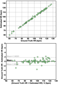
(a) SSPD (ours)

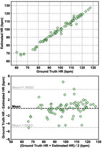
(b) Contrast-Phys [5]

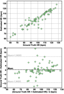
(c) RemotePPG [23]

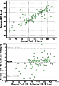
(d) ICA [18]

Figure 6: The scatter (top) and Bland-Altman plots (bottom) illustrate the correlation between ground truth HR and estimated HR on the UBFC-rPPG dataset.

TABLE III: HRV and RF estimation results on the UBFC-rPPG dataset compared to the state-of-the-art methods. The best results are highlighted in bold. The notation “-L3” indicates that the temporal similarity pyramid consists of three layers.

		LF (n.u.)			HF (n.u.)			LF / HF			RF (Hz)
Method Types	Methods	SD$\downarrow$	RMSE$\downarrow$	R$\uparrow$	SD$\downarrow$	RMSE$\downarrow$	R$\uparrow$	SD$\downarrow$	RMSE$\downarrow$	R$\uparrow$	SD$\downarrow$	RMSE$\downarrow$	R$\uparrow$
Traditional	GREEN [20]	0.186	0.186	0.280	0.186	0.186	0.280	0.361	0.365	0.492	0.087	0.086	0.111
	POS [21]	0.171	0.169	0.479	0.171	0.169	0.479	0.405	0.399	0.518	0.109	0.107	0.087
	CHROM [19]	0.214	0.378	0.188	0.214	0.378	0.188	0.631	0.800	0.151	0.091	0.092	0.074
	ICA [18]	0.243	0.240	0.159	0.243	0.240	0.159	0.655	0.645	0.226	0.086	0.089	0.102
Supervised	CVD [53]	0.053	0.065	0.740	0.053	0.065	0.740	0.169	0.168	0.812	0.017	0.018	0.252
	Dual-GAN [3]	0.034	0.035	0.891	0.034	0.035	0.891	0.131	0.136	0.881	0.010	0.010	0.395
Unsupervised	RemotePPG [23]	0.091	0.139	0.694	0.091	0.139	0.694	0.525	0.691	0.684	0.061	0.098	0.103
	Contrast-Phys [5]	0.050	0.098	0.798	0.050	0.098	0.798	0.205	0.395	0.782	0.055	0.083	0.347
	SSPD-L3	0.047	0.062	0.822	0.047	0.062	0.822	0.282	0.318	0.806	0.044	0.042	0.361

IV Experiments

IV-A Datasets and Metrics

We conduct experiments on four commonly used open-access benchmarks: PURE [15], UBFC-rPPG [16], VIPL-HR [9], and MR-NIRP [10]. Specifically, PURE [15] consists of 10 persons with 6 different head motion types. We adopt the pre-defined strategy that aligns with previous works [5, 63] to split the training and test sets. UBFC-rPPG [16] comprises 42 subjects who are asked to play a mathematical game to elicit varied HRs. We follow the protocol established by the dataset author to split the training and test sets, which is consistent with [3, 5]. VIPL-HR [9] is a challenging large-scale benchmark for remote physiological measurement, it contains 9 scenarios for 107 subjects with different head movements, illumination changes, and recording devices. We use a subject-exclusive 5-fold cross-validation protocol in line with the [3, 4]. MR-NIRP [10] is another challenging dataset due to the low intensity of the rPPG signals in NIR videos. This dataset comprises 8 subjects and 2 experiments (still and motion), and we implement the subject-exclusive 8-fold cross-validation strategy as utilized in [5].

We apply the widely used evaluation metrics in remote HR measurement [60], including mean absolute error (MAE), root mean square error (RMSE), standard deviation (SD), and Pearson’s correlation coefficient (R). We detect all the peaks [66] in the estimated rPPG waveform, and the HR is determined based on the averaged peak intervals. Furthermore, we extract low-frequency power (LF) in normalized units (n.u.), high-frequency power (HF) in normalized units (n.u.), the LF/HF power ratio, and respiration frequency (RF) features using the method implemented in [67]. Following [5], we report SD, RMSE, and R metrics to evaluate the HRV estimation performance.

IV-B Implementation Details

Our framework is implemented on an NVIDIA GeForce RTX 3090 GPU using Pytorch 1.7.1. We train the model for 50 epochs via Adam optimizer [68] with no weight decay, and the learning rate is 0.001. We set the initial and ending momentum rate to 0.9 and 1.0, respectively, which is scheduled by cosine annealing [69]. In the training stage, 10s video clips with a size of $128\times 128$ are selected randomly from the input video, with a batch size of 12. During inference, we strictly follow the previous works [4, 5] and the rPPG waveform is typically predicted from each 30s non-overlapping clip in the test set unless otherwise indicated.

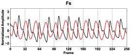
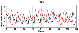
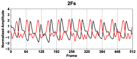
(a) SSPD-L3 (ours)

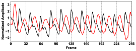
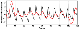
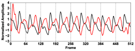
(b) Contrast-Phys [5]

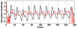
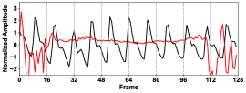
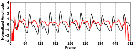
(c) RemotePPG [23]

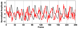
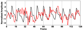
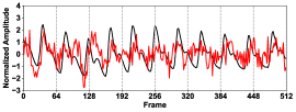
(d) ICA [18]

Figure 7: The rPPG waveform predictions on the first subject in the test set of the PURE dataset. We input the same clip with different sampling rates, namely $F_{s}$ (left column), $F_{s}/2$ (middle column), and $2F_{s}$ (right column), to the same model. The red lines represent the rPPG predictions, while the black lines represent the corresponding BVP labels. Note that all results are derived directly from the model’s output without any filtering.

IV-C Comparison with the State-of-the-art

IV-C1 Intra-dataset Testing

Firstly, we perform intra-dataset evaluations for HR estimation on three small-scale benchmarks. As demonstrated in Table I, our framework outperforms all the signal-based and learning-based unsupervised methods with a substantial improvement. Here, “L3” denotes that the $S^{3}M$ contains three TS blocks, i.e., the temporal similarity pyramid consists of three layers. In the PURE dataset, SSPD-L3 achieves higher performance than the current state-of-the-art supervised model [3], while in the UBFC-rPPG and MR-NIRP datasets, SSPD-L3 exhibits comparable results to the state-of-the-art supervised model [5]. For a more intuitive illustration of the performance of our method, we first reproduce three competitive unsupervised baselines: Contrast-Phys [5], RemotePPG [23], and ICA [18] (the best signal-based method), and generate regression and Bland-Altman plots on the UBFC-rPPG dataset. Fig. 6 shows that our framework displays the strongest correlation with the ground truth and the lowest standard deviation of errors, indicating that SSPD achieves the most precise and stable unsupervised HR measurement. Besides, in Fig. 7, we showcase the rPPG estimation obtained from the first subject in the test set on the PURE dataset. It can be easily observed that the output of the proposed SSPD framework maintains a consistent phase shift with the BVP label across different sampling rates. Particularly, in a low sampling rate, SSPD exhibits robustness to information reductions, enabling it to maintain highly confident output peaks that are synchronized with the label and result in precise HR estimation. Meanwhile, in a high sampling rate, SSPD can preserve accurate rhythm w.r.t. the BVP label while simultaneously capturing more subtle waveform dynamics, such as the diastolic peaks [49]. This toy experiment demonstrates that our SSPD framework outperforms other unsupervised baselines, especially in the presence of sampling rate jitter. The efficacy of SSPD can be attributed to its capacity to acquire self-similar physiological features across multi-scale and long-distance intervals, which enables robustness to frequency perturbations and accurate prediction of extreme heart rates. Note that all waveforms are performed directly on the models’ output without any filtering, and the observed phase shift between the predicted rPPG and the BVP label is attributed to the lack of manual alignment.

Next, we report the HR estimation results in the challenging VIPL-HR dataset in Table II. It should be highlighted that the previous unsupervised baseline [26] utilized a distinct test protocol, where they only assessed the performance on fold-1 of the VIPL-HR dataset, and each clip was limited to 160 frames to predict nearly instantaneous heart rate. To ensure a fair comparison, we follow the aforementioned protocol and present the performance of the SSPD-L3-160 model, whereas the SSPD-L3 model follows the strategy in line with the [4]. Noteworthy, ViViT [26] used the linear probe strategy to fine-tune their unsupervised model, while all of our results are obtained without any supervision. Furthermore, we reproduce two solid unsupervised baselines [5, 23] on the VIPL-HR dataset based on open-source codes. As shown in Table II, our SSPD-L3 model significantly outperforms Contrast-Phys using the same test strategy, indicating that the self-similarity prior facilitates the model to effectively capture physiological features, especially in large and complex datasets. In addition, we visualize the error distributions for 9 different tasks across all subjects in the VIPL-HR dataset. The boxplot in Fig. 5 reveals that SSPD has notably lower errors compared to the unsupervised state-of-the-art model [5] and performs comparably to the supervised state-of-the-art model [3] in most scenarios, especially in the task1: stable scenario, task4: bright scenario, task6: long distance scenario, and task8: phone stable scenario. The results demonstrate that our framework achieves the best performance in unsupervised models, narrowing the gap between unsupervised and supervised methods.

Finally, we conduct intra-dataset HRV testing on the UBFC-rPPG dataset. Experimental results in Table. III demonstrates that SSPD outperforms the state-of-the-art unsupervised methods [5], evident from the significantly lower RMSE in LF, HF, and RF estimation. The superior performance in both HR and HRV measurement indicates that SSPD excels not only in accurately predicting average peak intervals but also in precisely locating individual peaks, resulting in the high-quality construction of rPPG signals.

To sum up, the proposed SSPD framework demonstrates high confidence in HR, HRV, and RF estimation, providing evidence for the potential of unsupervised remote physiological measurement to outperform supervised counterparts.

IV-C2 Cross-dataset Testing

We conduct cross-dataset evaluations to exhibit the generalization of our framework. In Table I, we present the HR estimation results obtained by selecting the best fold-2 trained on VIPL-HR and testing it on PURE, UBFC-rPPG, and MR-NIRP. We directly compare them to the intra-dataset results, and our framework performs on par with the unsupervised state-of-the-art method. The cross-dataset evaluations demonstrate that SSPD can learn intrinsic self-similarity as a domain-invariant [67, 70] characteristic presented in various inputs, and it is insensitive to distributional differences among datasets.

TABLE IV: The compute cost and running speed compared to the state-of-the-art end-to-end methods. The last column reports the HR estimation performance on the PURE dataset, and the best results are highlighted in bold. The ^★ indicates the incorporation of the frame difference calculation process.

Method Types	Methods	Params	GFLOPs	Time	MAE$\downarrow$
Supervised	PhysNet [13]	0.77M	131.47	$\times$1.00	2.10
	CAN★ [12]	7.50M	225.01	$\times$3.19	1.27
	PhysFormer [4]	7.38M	94.89	$\times$2.91	-
Unsupervised	RemotePPG [23]	0.86M	256.68	$\times$1.88	2.30
	Contrast-Phys [5]	0.86M	256.68	$\times$1.88	1.00
	SSPD★	0.78M	84.79	$\times$1.00	0.53

IV-C3 Inference Cost

To demonstrate the effectiveness of the proposed self-similarity-aware network, particularly the design of the $S^{3}M$, we first reproduce the end-to-end rPPG baselines based on open-source codes [4, 5, 23, 71], then we calculate the computational complexity and actual inference time under the same hardware environment, as shown in Table IV. The input size for all tests is 300$\times$128$\times$128 and the running time is obtained by averaging 10 independent tests. It should be noted that the running time additionally includes the frame difference calculation in both CAN [12] and SSPD for a fair comparison. According to Table IV, our framework achieves the lowest compute cost and the fastest running speed during inference while maintaining the best performance. Specifically, compared to the current unsupervised state-of-the-art model [5], our method has almost 3$\times$ fewer GFLOPs and 2$\times$ less inference time, while the end-to-end supervised state-of-the-art model [4] has nearly 10$\times$ parameters and 3$\times$ more inference time than ours. Thus, our method is carbon-neutral, making it suitable for embedded and edge computing platforms.

TABLE V: Ablation studies on hierarchical self-distillation and complementary regularizations in our SSPD framework. The best results are highlighted in bold.

Methods	$\mathcal{L}_{SD}$	$\mathcal{L}_{Distill}$		$\mathcal{L}_{SNR}$	MAE$\downarrow$	RMSE$\downarrow$	R$\uparrow$
		$\mathcal{L}_{RPD}$	$\mathcal{L}_{TSPD}$
w/o TSPD	-	✓	-	-	1.26	3.55	0.955
w/o RPD	-	-	✓	-	1.51	2.40	0.981
$\mathcal{L}_{Distill}$ only	-	✓	✓	-	0.72	1.21	0.991
w/o $\mathcal{L}_{SD}$	-	✓	✓	✓	0.79	1.36	0.992
w/o $\mathcal{L}_{SNR}$	✓	✓	✓	-	0.78	1.14	0.995
default	✓	✓	✓	✓	0.50	0.71	0.998

IV-D Ablation Studies

In this section, we conduct comprehensive ablation studies on the UBFC-rPPG dataset to investigate the effectiveness of the SSPD framework.

IV-D1 Hierarchical Self-distillation

Initially, we explore the importance of two distilled knowledge in the SSPD framework. The upper part of Table V shows that dropping either the Temporal Similarity Pyramid Distillation (TSPD) or RPPG Prediction Distillation (RPD) leads to significant performance degradation. The best performance is achieved when both TSPD and RPD are leveraged simultaneously, indicating that two distilled knowledge from both signal and latent spaces complement each other. Next, Fig. 8(a) illustrates the importance of the initial momentum rate in EMA, as defined in Eqn. 13. Results show that a relatively small momentum rate benefits model learning. Empirically, an initial momentum rate of 0.9 is found to be optimal for small-scale datasets, while 0.99 is more suitable for the larger VIPL-HR dataset.

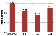
(a) momentum rate $\rho$

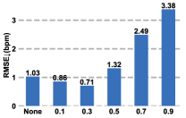
(b) mask ratio $p$

Figure 8: The effects of hyperparameters, including (a) momentum rate $\rho$ and (b) mask ratio $p$, on the proposed SSPD framework.

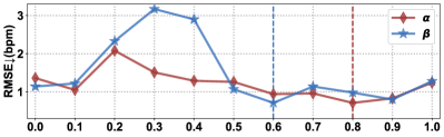
Figure 9: Impacts of the hyperparameters (a) $\alpha$, (b) $\beta$ on the tradeoff between two complementary regularizations.

IV-D2 Complementary Regularizations

As demonstrated in the lower part of Table V, the SD regularization and the SNR regularization in the SSPD framework are also complementary. Solely applying the SD or SNR regularization based on self-distillation leads to a slightly higher error, while combining both achieves the optimal performance. The reason for this is that each regularization has a different learning direction relative to self-distillation, and only integrating two directions boosts the effectiveness of self-distillation. To further investigate the tradeoff between SD regularization and SNR regularization, we perform a grid search for hyperparameters $\alpha$ and $\beta$, as presented in Eqn. 12. Based on the results in Fig. 9, we set $\alpha$ and $\beta$ to 0.8 and 0.6 by default, respectively.

TABLE VI: Ablation studies on the physical-prior embedded augmentation and the application of stop-gradient in the predictor module. The best results are highlighted in bold.

Methods	MAE$\downarrow$	RMSE$\downarrow$	R$\uparrow$
w/o LGA	1.09	2.15	0.981
w/o frame difference mapping in MDM	4.15	6.10	0.842
w/o random masking in MDM	0.63	1.03	0.995
predictor module w/o stop-gradient	0.77	1.13	0.995
default	0.50	0.71	0.998

TABLE VII: Ablation studies on the architecture of the TS block. The best results are highlighted in bold.

Methods	MAE$\downarrow$	RMSE$\downarrow$	R$\uparrow$
w/o residual connection	1.07	2.13	0.980
w/o dot-product attention	0.81	1.21	0.994
w/o projection	0.55	0.78	0.997
dot-product attention $\rightarrow$ self-attention	0.71	1.03	0.995
multi-head $\rightarrow$ single-head	0.69	1.00	0.996
default	0.50	0.71	0.998

TABLE VIII: Ablation studies on the input shape of the SSPD framework, the number of layers, and the token size in $S^{3}M$. The best results are highlighted in bold.

Methods	Input Size	Token Size	MAE$\downarrow$	RMSE$\downarrow$	R$\uparrow$
SSPD-L1	300$\times$128$\times$128	$\left[292\times 256\right]$	0.73	1.46	0.991
SSPD-L2	300$\times$128$\times$128	$\left[292\times 256\right]$ $\left[286\times 256\right]$	0.60	0.94	0.996
SSPD-L3	300$\times$128$\times$128	$\left[292\times 128\right]$ $\left[286\times 128\right]$ $\left[282\times 128\right]$	0.55	0.79	0.998
SSPD-L3	300$\times$128$\times$128	$\left[292\times 256\right]$ $\left[286\times 256\right]$ $\left[282\times 256\right]$	0.50	0.71	0.998
SSPD-L3	300$\times$128$\times$128	$\left[292\times 512\right]$ $\left[286\times 512\right]$ $\left[282\times 512\right]$	0.50	0.72	0.998
SSPD-L3	300$\times$128$\times$128	$\left[296\times 256\right]$ $\left[144\times 256\right]$ $\left[68\times 256\right]$	0.69	1.01	0.995
SSPD-L3	160$\times$128$\times$128	$\left[152\times 256\right]$ $\left[146\times 256\right]$ $\left[142\times 256\right]$	0.54	0.79	0.997
SSPD-L3	300$\times$96$\times$96	$\left[292\times 256\right]$ $\left[286\times 256\right]$ $\left[282\times 256\right]$	0.60	0.85	0.996
SSPD-L4	300$\times$128$\times$128	$\left[292\times 256\right]$ $\left[286\times 256\right]$ $\left[282\times 256\right]$ $\left[280\times 256\right]$	0.54	0.76	0.997

IV-D3 Physical-prior Embedded Augmentation

The results presented in Table VI exhibit the impact of two physical-prior embedded augmentation strategies. Specifically, Local-Global Augmentation (LGA) is crucial in enhancing the local-global response, thus improving modeling capability at different spatial resolutions. On the other hand, Masked Difference Modeling (MDM) further increases the deviation between two augmented views and benefits self-similarity-aware learning. It is worth noting that frame difference mapping is a crucial component of MDM (-3.65 bpm MAE), with its ability to enable the model to concentrate on motion information while preventing model collapse. Nevertheless, incorporating random masking in MDM can further improve the estimation accuracy based on the aforementioned techniques. In addition, we search for the optimal mask ratio, as shown in Fig 8(b). The results indicate that a mask ratio of 0.3 yields the best performance, while overly high mask ratios result in dramatic degradation. To sum up, we propose two physical-prior embedded augmentation strategies to enhance the model’s performance from different perspectives.

IV-D4 Stop-gradient in Predictor Module

The fourth row in Table VI shows the effectiveness of the stop-gradient in the predictor (-0.27 bpm MAE), indicating the existence of a conflict between the learning of self-similar representations and the construction of rPPG waveform. This experiment suggests that the predictor module is better suited as a plug-and-play module designed for downstream tasks through fine-tuning.

IV-D5 TS Block

In Table VII, we conduct a comprehensive analysis on the components of the TS block. The first two rows show that the residual connection and dot-product attention are the most crucial elements of the block. That is because residual connection enhances the capturing of self-similar representations across multiple time scales, while the attention mechanism enhances the long-distance physiological features learning within each specific time scale. Furthermore, dot-product attention, as defined in Eqn. 2, and multi-head attention outperform self-attention and single-head attention, respectively. Finally, the projection module following the multi-head attention further boosts the performance by fusing the information from different heads.

IV-D6 Self-similarity-aware Network

In our investigation of the implementation of the self-similarity-aware network, we explore multiple factors, including the input shape of the SSPD framework, as well as the number of layers and token size in the $S^{3}M$. The results are illustrated in Table VIII, which can be summarized as follows: (a) The incorporation of multiple time scales improves the performance of the network. By comparing the results obtained with different numbers of layers in the temporal similarity pyramid, we observe that the performance boosts with an increasing number of layers, and then reaches saturation at SSPD-L4. Moreover, the computational cost of training significantly increases with the number of blocks, hence we use SSPD-L3 by default. (b) The self-similarity-aware network is insensitive to the dimension of token embeddings. As evidenced by the results in rows three to five of Table VIII, there is little variation in the MAE, RMSE, and R metrics despite an increase in dimension from 128 to 512. Nevertheless, to achieve the optimal balance between performance and speed, we set the dimension to 256. (c) A dramatic change in time scales leads to degradation. To address this issue, we employ an adaptive average pooling layer in the tokenizer of each TS block, where the time scale is reduced by half at each layer of the pyramid. As shown in the sixth row of Table VIII, the MAE increases from 0.5 to 0.69 due to the dramatic changes in time scales. The reduced granularity of self-similar representations in the time domain can result in decreased accuracy in rPPG estimation, and also potentially reduce the efficacy of the SNR regularization due to the lowered spectral resolution. (d) The self-similarity-aware network exhibits robustness to variations in input shape. Specifically, we evaluate the impact of reducing the temporal length of the input clips from 300 to 160 and the spatial size from 128$\times$128 to 96$\times$96. Our results show a slight decrease in performance due to the reduced shape in both space and time domains. Nonetheless, the SSPD framework maintains its state-of-the-art performance in unsupervised methods.

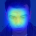
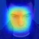
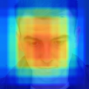
(a)

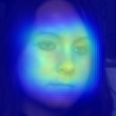
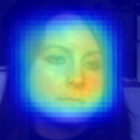
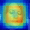
(b) (a) Saliency maps generated from different convolutional layers in the SSPD backbone on the UBFC-rPPG (top) and PURE (bottom) datasets. Each map, from left to right, corresponds to ConvBlock1_Conv2, ConvBlock2_Conv2, and ConvBlock3_Conv2, respectively.

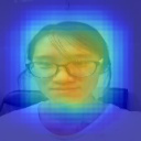
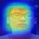
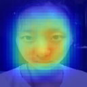
(c) (b) Saliency maps generated from three subjects in the VIPL-HR dataset using ConvBlock2_Conv2.

Figure 10: Saliency maps generated from different convolutional layers and subjects in multiple datasets during the inference stage by SSPD.

IV-E Interpretability

In Fig. 10, we generate saliency maps during the inference stage based on LayerCAM [72]. Specifically, we first train our SSPD model in an unsupervised manner. Subsequently, we employ BVP ground truth and the negative Pearson loss ($\mathcal{L}_{Pearson}(\cdot)$) to compute gradients for multiple convolutional layers within the backbone. Finally, we follow the LayerCAM to derive the gradient-weighted activation map $\mathcal{M}_{i}\in\mathbb{R}^{T\times H_{i}\times W_{i}}$ for the i-th layer. Noteworthy, for visualization purposes, we average the $\mathcal{M}_{i}$ along the temporal dimension to obtain $\widetilde{\mathcal{M}_{i}}\in\mathbb{R}^{H_{i}\times W_{i}}$. Then, we combine it with the first input frame to establish spatial correspondence. The first two rows in Fig. 10 are generated from different convolutional layers in the UBFC-rPPG and PURE datasets. From left to right, they correspond to ConvBlock1_Conv2, ConvBlock2_Conv2, and ConvBlock3_Conv2, respectively. It can be observed that as we move from shallow to deep layers, SSPD concentrates more on the facial area rather than the background, especially in the cheek and forehead regions. This behavior aligns with the physiological prior [4, 6]. Moreover, the saliency maps in the last row of Fig. 10, obtained from three subjects in the VIPL-HR dataset using ConvBlock2_Conv2 (chosen for its favorable balance between spatial resolution and semantic information), exhibit the same phenomenon. SSPD consistently directs attention to areas with a high prior intensity of facial blood flow, enhancing its interpretability in remote physiological measurement.

V Conclusions and Future Work

In this paper, we propose the self-distillation framework SSPD for unsupervised remote physiological measurement, which capitalizes on the intrinsic self-similarity of cardiac activities. To disentangle self-similar physiological features from facial videos, we first introduce a physical-prior embedded augmentation technique. Then, we tailor a self-similarity-aware network with a separable self-similarity model. Finally, we develop a hierarchical self-distillation paradigm. The experimental results demonstrate that SSPD achieves comparable or even superior performance compared to state-of-the-art supervised methods and serves as a strong yet efficient baseline for unsupervised rPPG estimation. Our future work includes: (1) Exploring the effectiveness of spatial self-similarity for modeling facial blood flow and achieving more precise physiological measurements. (2) Leveraging the self-distillation framework to fine-tune multiple downstream tasks, such as atrial fibrillation detection, fatigue judgment, and emotion recognition.

References

- [1] L. Mou, C. Zhou, P. Xie, P. Zhao, R. C. Jain, W. Gao, and B. Yin, “Isotropic self-supervised learning for driver drowsiness detection with attention-based multimodal fusion,” IEEE Transactions on Multimedia, 2021.
- [2] C.-H. Cheng, K.-L. Wong, J.-W. Chin, T.-T. Chan, and R. H. So, “Deep learning methods for remote heart rate measurement: A review and future research agenda,” Sensors, vol. 21, no. 18, p. 6296, 2021.
- [3] H. Lu, H. Han, and S. K. Zhou, “Dual-gan: Joint bvp and noise modeling for remote physiological measurement,” in Proceedings of the IEEE/CVF Conference on Computer Vision and Pattern Recognition, 2021, pp. 12 404–12 413.
- [4] Z. Yu, Y. Shen, J. Shi, H. Zhao, P. H. Torr, and G. Zhao, “Physformer: facial video-based physiological measurement with temporal difference transformer,” in Proceedings of the IEEE/CVF Conference on Computer Vision and Pattern Recognition, 2022, pp. 4186–4196.
- [5] Z. Sun and X. Li, “Contrast-phys: Unsupervised video-based remote physiological measurement via spatiotemporal contrast,” in Computer Vision–ECCV 2022: 17th European Conference, Tel Aviv, Israel, October 23–27, 2022, Proceedings, Part XII. Springer, 2022, pp. 492–510.
- [6] W. Chen and D. McDuff, “Deepphys: Video-based physiological measurement using convolutional attention networks,” in Proceedings of the european conference on computer vision, 2018, pp. 349–365.
- [7] X. Niu, S. Shan, H. Han, and X. Chen, “Rhythmnet: End-to-end heart rate estimation from face via spatial-temporal representation,” IEEE Transactions on Image Processing, vol. 29, pp. 2409–2423, 2019.
- [8] Z. Yu, W. Peng, X. Li, X. Hong, and G. Zhao, “Remote heart rate measurement from highly compressed facial videos: an end-to-end deep learning solution with video enhancement,” 07 2019.
- [9] X. Niu, S. Shan, H. Han, and X. Chen, “Rhythmnet: End-to-end heart rate estimation from face via spatial-temporal representation,” IEEE Transactions on Image Processing, vol. 29, pp. 2409–2423, 2019.
- [10] E. Magdalena Nowara, T. K. Marks, H. Mansour, and A. Veeraraghavan, “Sparseppg: Towards driver monitoring using camera-based vital signs estimation in near-infrared,” in Proceedings of the IEEE conference on computer vision and pattern recognition workshops, 2018, pp. 1272–1281.
- [11] M. Soleymani, J. Lichtenauer, T. Pun, and M. Pantic, “A multimodal database for affect recognition and implicit tagging,” IEEE Transactions on Affective Computing, vol. 3, no. 1, pp. 42–55, 2012.
- [12] X. Liu, J. Fromm, S. Patel, and D. McDuff, “Multi-task temporal shift attention networks for on-device contactless vitals measurement,” Advances in Neural Information Processing Systems, vol. 33, pp. 19 400–19 411, 2020.
- [13] Z. Yu, X. Li, and G. Zhao, “Remote photoplethysmograph signal measurement from facial videos using spatio-temporal networks,” arXiv preprint arXiv:1905.02419, 2019.
- [14] X. Niu, H. Hu, S. Shan, and X. Chen, “Synrhythm: Learning a deep heart rate estimator from general to specific,” in International Conference on Pattern Recognition, 2018.
- [15] R. Stricker, S. Müller, and H.-M. Gross, “Non-contact video-based pulse rate measurement on a mobile service robot,” in The 23rd IEEE International Symposium on Robot and Human Interactive Communication. IEEE, 2014, pp. 1056–1062.
- [16] S. Bobbia, R. Macwan, Y. Benezeth, A. Mansouri, and J. Dubois, “Unsupervised skin tissue segmentation for remote photoplethysmography,” Pattern Recognition Letters, vol. 124, pp. 82–90, 2019.
- [17] T. Zhang, A. El Ali, A. Hanjalic, and P. Cesar, “Few-shot learning for fine-grained emotion recognition using physiological signals,” IEEE Transactions on Multimedia, 2022.
- [18] M.-Z. Poh, D. J. McDuff, and R. W. Picard, “Non-contact, automated cardiac pulse measurements using video imaging and blind source separation.” Optics express, vol. 18, no. 10, pp. 10 762–10 774, 2010.
- [19] G. De Haan and V. Jeanne, “Robust pulse rate from chrominance-based rppg,” IEEE Transactions on Biomedical Engineering, vol. 60, no. 10, pp. 2878–2886, 2013.
- [20] W. Verkruysse, L. O. Svaasand, and J. S. Nelson, “Remote plethysmographic imaging using ambient light.” Optics express, vol. 16, no. 26, pp. 21 434–21 445, 2008.
- [21] W. Wang, A. C. Den Brinker, S. Stuijk, and G. De Haan, “Algorithmic principles of remote ppg,” IEEE Transactions on Biomedical Engineering, vol. 64, no. 7, pp. 1479–1491, 2016.
- [22] Z. Hasan, A. Z. M. Faridee, M. Ahmed, and N. Roy, “Self-rppg: Learning the optical & physiological mechanics of remote photoplethysmography with self-supervision,” in 2022 IEEE/ACM Conference on Connected Health: Applications, Systems and Engineering Technologies. IEEE, 2022, pp. 46–56.
- [23] J. Gideon and S. Stent, “The way to my heart is through contrastive learning: Remote photoplethysmography from unlabelled video,” in Proceedings of the IEEE/CVF International Conference on Computer Vision, October 2021, pp. 3995–4004.
- [24] Z. Yue, M. Shi, and S. Ding, “Video-based remote physiological measurement via self-supervised learning,” arXiv preprint arXiv:2210.15401, 2022.
- [25] H. Wang, E. Ahn, and J. Kim, “Self-supervised representation learning framework for remote physiological measurement using spatiotemporal augmentation loss,” in Proceedings of the AAAI Conference on Artificial Intelligence, vol. 36, no. 2, 2022, pp. 2431–2439.
- [26] S. Park, B.-K. Kim, and S.-Y. Dong, “Self-supervised rgb-nir fusion video vision transformer framework for rppg estimation,” IEEE Transactions on Instrumentation and Measurement, vol. 71, pp. 1–10, 2022.
- [27] W. Sun and Q. Sun, “Non-contact measurement of physiological parameters based on contrastive learning,” in 2022 4th International Conference on Frontiers Technology of Information and Computer. IEEE, 2022, pp. 445–449.
- [28] T. Lei, “Similarity between the mandelbrot set and julia sets,” Communications in mathematical physics, vol. 134, pp. 587–617, 1990.
- [29] J. Devlin, M.-W. Chang, K. Lee, and K. Toutanova, “Bert: Pre-training of deep bidirectional transformers for language understanding,” arXiv preprint arXiv:1810.04805, 2018.
- [30] A. Radford, K. Narasimhan, T. Salimans, I. Sutskever et al., “Improving language understanding by generative pre-training,” 2018.
- [31] K. He, H. Fan, Y. Wu, S. Xie, and R. Girshick, “Momentum contrast for unsupervised visual representation learning,” in Proceedings of the IEEE/CVF conference on computer vision and pattern recognition, 2020, pp. 9729–9738.
- [32] K. He, X. Chen, S. Xie, Y. Li, P. Dollár, and R. Girshick, “Masked autoencoders are scalable vision learners,” in Proceedings of the IEEE/CVF Conference on Computer Vision and Pattern Recognition, 2022, pp. 16 000–16 009.
- [33] M. Caron, H. Touvron, I. Misra, H. Jégou, J. Mairal, P. Bojanowski, and A. Joulin, “Emerging properties in self-supervised vision transformers,” in Proceedings of the IEEE/CVF International Conference on Computer Vision, 2021, pp. 9650–9660.
- [34] S. Chopra, R. Hadsell, and Y. LeCun, “Learning a similarity metric discriminatively, with application to face verification,” in 2005 IEEE Computer Society Conference on Computer Vision and Pattern Recognition, vol. 1. IEEE, 2005, pp. 539–546.
- [35] T. Chen, S. Kornblith, M. Norouzi, and G. Hinton, “A simple framework for contrastive learning of visual representations,” in International conference on machine learning. PMLR, 2020, pp. 1597–1607.
- [36] T. Gao, X. Yao, and D. Chen, “Simcse: Simple contrastive learning of sentence embeddings,” 2022.
- [37] H. Bao, L. Dong, S. Piao, and F. Wei, “Beit: Bert pre-training of image transformers,” arXiv preprint arXiv:2106.08254, 2021.
- [38] M. Assran, M. Caron, I. Misra, P. Bojanowski, F. Bordes, P. Vincent, A. Joulin, M. Rabbat, and N. Ballas, “Masked siamese networks for label-efficient learning,” in Computer Vision–ECCV 2022: 17th European Conference, Tel Aviv, Israel, October 23–27, 2022, Proceedings, Part XXXI. Springer, 2022, pp. 456–473.
- [39] J. Zhou, C. Wei, H. Wang, W. Shen, C. Xie, A. Yuille, and T. Kong, “ibot: Image bert pre-training with online tokenizer,” arXiv preprint arXiv:2111.07832, 2021.
- [40] R. Hadsell, S. Chopra, and Y. LeCun, “Dimensionality reduction by learning an invariant mapping,” in 2006 IEEE Computer Society Conference on Computer Vision and Pattern Recognition, vol. 2. IEEE, 2006, pp. 1735–1742.
- [41] J.-B. Grill, F. Strub, F. Altché, C. Tallec, P. Richemond, E. Buchatskaya, C. Doersch, B. Avila Pires, Z. Guo, M. Gheshlaghi Azar et al., “Bootstrap your own latent-a new approach to self-supervised learning,” Advances in neural information processing systems, vol. 33, pp. 21 271–21 284, 2020.
- [42] G. Hinton, O. Vinyals, and J. Dean, “Distilling the knowledge in a neural network,” arXiv preprint arXiv:1503.02531, 2015.
- [43] Z. Hao, Y. Luo, Z. Wang, H. Hu, and J. An, “Cdfkd-mfs: Collaborative data-free knowledge distillation via multi-level feature sharing,” IEEE Transactions on Multimedia, vol. 24, pp. 4262–4274, 2022.
- [44] Z. Wu, Y. Xiong, S. X. Yu, and D. Lin, “Unsupervised feature learning via non-parametric instance discrimination,” in Proceedings of the IEEE conference on computer vision and pattern recognition, 2018, pp. 3733–3742.
- [45] M. Caron, I. Misra, J. Mairal, P. Goyal, P. Bojanowski, and A. Joulin, “Unsupervised learning of visual features by contrasting cluster assignments,” Advances in neural information processing systems, vol. 33, pp. 9912–9924, 2020.
- [46] M. Lewandowska, J. Rumiński, T. Kocejko, and J. Nowak, “Measuring pulse rate with a webcam — a non-contact method for evaluating cardiac activity,” in 2011 Federated Conference on Computer Science and Information Systems, 2011, pp. 405–410.
- [47] C. Yang, G. Cheung, and V. Stankovic, “Estimating heart rate and rhythm via 3d motion tracking in depth video,” IEEE Transactions on Multimedia, vol. 19, no. 7, pp. 1625–1636, 2017.
- [48] K. Simonyan and A. Zisserman, “Two-stream convolutional networks for action recognition in videos,” Advances in neural information processing systems, vol. 27, 2014.
- [49] E. Nowara, D. McDuff, and A. Veeraraghavan, “The benefit of distraction: Denoising remote vitals measurements using inverse attention,” arXiv preprint arXiv:2010.07770, 2020.
- [50] J. Kang, S. Yang, and W. Zhang, “Transppg: Two-stream transformer for remote heart rate estimate,” arXiv preprint arXiv:2201.10873, 2022.
- [51] D. Huang, X. Feng, H. Zhang, Z. Yu, J. Peng, G. Zhao, and Z. Xia, “Spatio-temporal pain estimation network with measuring pseudo heart rate gain,” IEEE Transactions on Multimedia, vol. 24, pp. 3300–3313, 2021.
- [52] A. Dosovitskiy, L. Beyer, A. Kolesnikov, D. Weissenborn, X. Zhai, T. Unterthiner, M. Dehghani, M. Minderer, G. Heigold, S. Gelly et al., “An image is worth 16x16 words: Transformers for image recognition at scale,” arXiv preprint arXiv:2010.11929, 2020.
- [53] X. Niu, Z. Yu, H. Han, X. Li, S. Shan, and G. Zhao, “Video-based remote physiological measurement via cross-verified feature disentangling,” in Computer Vision–ECCV 2020: 16th European Conference, Glasgow, UK, August 23–28, 2020, Proceedings, Part II 16. Springer, 2020, pp. 295–310.
- [54] J. Deng, W. Dong, R. Socher, L.-J. Li, K. Li, and L. Fei-Fei, “Imagenet: A large-scale hierarchical image database,” in 2009 IEEE conference on computer vision and pattern recognition. Ieee, 2009, pp. 248–255.
- [55] J. Carreira, E. Noland, C. Hillier, and A. Zisserman, “A short note on the kinetics-700 human action dataset,” arXiv preprint arXiv:1907.06987, 2019.
- [56] V. Kazemi and J. Sullivan, “One millisecond face alignment with an ensemble of regression trees,” in Proceedings of the IEEE conference on computer vision and pattern recognition, 2014, pp. 1867–1874.
- [57] X. Wang, R. Girshick, A. Gupta, and K. He, “Non-local neural networks,” in Proceedings of the IEEE conference on computer vision and pattern recognition, 2018, pp. 7794–7803.
- [58] A. Vaswani, N. Shazeer, N. Parmar, J. Uszkoreit, L. Jones, A. N. Gomez, Ł. Kaiser, and I. Polosukhin, “Attention is all you need,” Advances in neural information processing systems, vol. 30, 2017.
- [59] K. He, X. Zhang, S. Ren, and J. Sun, “Deep residual learning for image recognition,” in Proceedings of the IEEE conference on computer vision and pattern recognition, 2016, pp. 770–778.
- [60] Y. Qiu, Y. Liu, J. Arteaga-Falconi, H. Dong, and A. El Saddik, “Evm-cnn: Real-time contactless heart rate estimation from facial video,” IEEE transactions on multimedia, vol. 21, no. 7, pp. 1778–1787, 2018.
- [61] Y. Yang, X. Liu, J. Wu, S. Borac, D. Katabi, M.-Z. Poh, and D. McDuff, “Simper: Simple self-supervised learning of periodic targets,” arXiv preprint arXiv:2210.03115, 2022.
- [62] E. Magdalena Nowara, T. K. Marks, H. Mansour, and A. Veeraraghavan, “Sparseppg: Towards driver monitoring using camera-based vital signs estimation in near-infrared,” in Proceedings of the IEEE conference on computer vision and pattern recognition workshops, 2018, pp. 1272–1281.
- [63] R. Spetlik, J. Cech, V. Franc, and J. Matas, “Visual heart rate estimation with convolutional neural network,” in BRITISH MACHINE VISION CONFERENCE, 2018.
- [64] R. Song, H. Chen, J. Cheng, C. Li, Y. Liu, and X. Chen, “Pulsegan: Learning to generate realistic pulse waveforms in remote photoplethysmography,” IEEE Journal of Biomedical and Health Informatics, vol. 25, no. 5, pp. 1373–1384, 2021.
- [65] E. M. Nowara, T. K. Marks, H. Mansour, and A. Veeraraghavan, “Near-infrared imaging photoplethysmography during driving,” IEEE Transactions on Intelligent Transportation Systems, vol. 23, no. 4, pp. 3589–3600, 2020.
- [66] P. Virtanen, R. Gommers, T. E. Oliphant, M. Haberland, T. Reddy, D. Cournapeau, E. Burovski, P. Peterson, W. Weckesser, J. Bright, S. J. van der Walt, M. Brett, J. Wilson, K. J. Millman, N. Mayorov, A. R. J. Nelson, E. Jones, R. Kern, E. Larson, C. J. Carey, İ. Polat, Y. Feng, E. W. Moore, J. VanderPlas, D. Laxalde, J. Perktold, R. Cimrman, I. Henriksen, E. A. Quintero, C. R. Harris, A. M. Archibald, A. H. Ribeiro, F. Pedregosa, P. van Mulbregt, and SciPy 1.0 Contributors, “SciPy 1.0: Fundamental Algorithms for Scientific Computing in Python,” Nature Methods, vol. 17, pp. 261–272, 2020.
- [67] H. Lu, Z. Yu, X. Niu, and Y.-C. Chen, “Neuron structure modeling for generalizable remote physiological measurement,” in Proceedings of the IEEE/CVF Conference on Computer Vision and Pattern Recognition, 2023, pp. 18 589–18 599.
- [68] M. D. Zeiler, “Adadelta: an adaptive learning rate method,” arXiv preprint arXiv:1212.5701, 2012.
- [69] I. Loshchilov and F. Hutter, “Sgdr: Stochastic gradient descent with warm restarts,” arXiv preprint arXiv:1608.03983, 2016.
- [70] W. Sun, X. Zhang, H. Lu, Y. Chen, Y. Ge, X. Huang, J. Yuan, and Y. Chen, “Resolve domain conflicts for generalizable remote physiological measurement,” in Proceedings of the 31st ACM International Conference on Multimedia, ser. MM ’23. New York, NY, USA: Association for Computing Machinery, 2023, pp. 8214–8224. [Online]. Available: https://doi.org/10.1145/3581783.3612265
- [71] X. Liu, X. Zhang, G. Narayanswamy, Y. Zhang, Y. Wang, S. Patel, and D. McDuff, “Deep physiological sensing toolbox,” arXiv preprint arXiv:2210.00716, 2022.
- [72] P.-T. Jiang, C.-B. Zhang, Q. Hou, M.-M. Cheng, and Y. Wei, “Layercam: Exploring hierarchical class activation maps for localization,” IEEE Transactions on Image Processing, vol. 30, pp. 5875–5888, 2021.