Floquet engineering of binding in doped and photo-doped Mott insulators
Abstract
We investigate the emergence of bound states in chemically and photo-doped Mott insulators, assisted by spin and -pairing fluctuations within both 2-leg ladder and 2D systems. We demonstrate that the binding energies and localization length in the chemically and photo-doped regimes are comparable. To effectively describe the photo and chemically doped state on the same footings, we employ the Schrieffer-Wolff transformation, resulting in a generalized - model. Furthermore, we show that manipulating the binding is possible through external periodic driving, a technique known as Floquet engineering, leading to significantly enhanced binding energies. We also roughly estimate the lifetime of photo-doped states under periodic driving conditions based on the Fermi golden rule. Lastly, we propose experimental protocols for realizing Hubbard excitons in cold-atom experiments.
I Introduction
Doped Mott insulators are one of the most intensively studied solid-state systems due to their significance for the high-temperature superconductors [1] and a plead of intriguing exotic phases including pseudogap [2, 3, 4],stripes [5, 6, 7], etc. One of the basic questions is how chemically doped charge carriers interact with the antiferromagnetic background, and it was proposed early on that carriers can form bound pairs whose binding energy originated from the shared distortion of the spin background (string-based pairing) [8, 9, 10, 11, 12, 13, 14, 15]. For the binding of charge carriers, the dimensionality of the system plays a particularly important role as in the purely 1D systems spin-charge separation prevents pairing [16, 17, 18, 19], making ladder [8, 20] and 2D systems [11, 15] minimal setups for studying of bound pairs. Experimental progress in cold atoms simulators enabled a direct observation of antiferromagnetic correlations [21], dressed spin polarons [22] and pairing strings [23, 24]. Furthermore, combining cold atom experiments and strong external fields enables a unique opportunity to manipulate microscopic parameters, like hopping and superexchange amplitude [25, 26]. Recent examples include enhanced binding of holes under a strong DC field in regimes where superexchange becomes comparable to the hopping integrals [27, 28], a situation not available in solid-state setups. These ideas stimulate exploring whether one could employ periodic (Floquet) driving [29, 30, 31], whose ability to manipulate microscopic parameters was already proved in cold-atoms experiments [32], to stabilize bound pairs in doped Mott insulators even further.
Photo doping of Mott insulators is an emerging direction to form exotic phases of matter [33, 34]. While the photo-doped systems are metastable, their lifetime can be exponentially long-lived for large gap Mott insulators [35, 36, 37, 38]. These states can exhibit novel non-thermal correlations, like the formation of Hubbard excitons [39, 40, 41, 42, 43, 44] or -pairing [45, 46, 47, 48, 49, 50, 51, 52], etc. In the high-dimensional systems, it was shown that -pairing fluctuations can lead to the condensation and form a superfluid [53], while in the one-dimensional setup a spin-charge- separation takes place [54]. An important open question is to establish what are the properties of photo-doped states beyond the two extreme case studies, like the ladders and 2D situation, as these are the most relevant experimental situations.
In this work, we compare the formation of a bound pair for chemically and photo-doped systems in the ladder and 2D geometries. To describe the chemically doped and metastable photo-doped systems on the same footing, we resort to the canonical transformation, which perturbatively decoupled sectors with different numbers of holons and doublons. We establish that the pairing due to spin and fluctuations does not compete or actively cooperate but rather leads to similar bindings between charge carriers in chemically and photo-doped systems. We provide an approximate measure of the binding energy for both chemically and photo-doped situations. Further, we show that periodic driving with an electromagnetic field enables an efficient manipulation of binding energies with its substantial increase for ladder and 2D systems and more localized charge distribution in real space. For photo-doped systems, we estimate the upper bound for the doublon-holon recombination rate in the presence of Floquet driving and proposed driving regimes where the exciton binding energies are larger than the lifetime. Finally, we comment on preparing photo-doped states in cold atom experiments by either chirped driving across the gap or adiabatic deformation of the lattice potential from band to Mott insulator.
II Model and method
We consider the Fermi Hubbard model
| (1) |
where sum runs over nearest neighbour pairs of sites, is the spin index denoting either up or down spin, is the hopping amplitude and the interaction strength. We will focus on the strong interaction limit , in which case the ground state at half-filling is the Mott insulating state. We will consider two different geometries with sites: (i) quasi one-dimension two-leg ladder with periodic boundary conditions along the elongated (chain) direction and (ii) two-dimensional lattice with periodic boundary conditions along both directions. The aim of our study is to understand and compare charge pairing and the role of spin and fluctuations in photo and chemically doped correlated systems.
While chemically doped systems are stable, the photo-doped situation for the large gap Mott insulator is only metastable with exponentially long lifetime [36, 35, 38, 55]. To treat the two scenarios on the same footing, we will perform a canonical Schrieffer-Wolf transformation which perturbatively decouples sectors with different number of effectively charged holons and doublons and obtain a generalized version of celebrated - Hamiltonian [56, 53, 47]. In the case of the photo-doped system, by neglecting higher-order recombination terms, we approximate the metastable state with an equilibrium state. Conveniently, such a description reduces the computational complexity. We then estimate the Hubbard exciton lifetime by Fermi golden rule in analogy with Ref. 38.
We denote the onsite interaction term in Eq. (1) with , and split the kinetic part into terms that preserves the number of doublon-holon (DH) pairs , that increases the number of DH pairs by one , and that decreases the number of DH pairs by one . Following Ref. 56, the generator of the unitary transformation is chosen such that it transforms out the processes that change the number of DH pairs on the order and retains them on the higher level of expansion. Hence, we choose such that and are cancelled (in Eq. (II)),
In the following, we distinguish the hopping amplitudes in x- and y-direction and denote them as and respectively. For 2D model, , as can be easily imposed in the following expressions. In the limit , we retain terms of the order , ) and neglect all higher orders, such that the effective Hamiltonian preserves the number of DH pairs
The terms act on the charge and spins along the x-direction (along the chain) whereas the terms act in the y-direction (along the rung for the two-leg model). When written out explicitly, the effective Hamiltonian has the following terms[47]
| (3) |
where and are the spin/ exchange coupling parameters along the chain and rung, respectively. When of the same strength, we drop the subscript and . The electron (hole) density per spin is given by , and is the complement of , i.e., if denotes up spin then denotes down spin and vice versa. The operators in terms of the fermion creation and annihilation operators can be expressed as , where is the vector to the th site and is a vector of the dimension of the system with entries . The component of the pseudospin is , , and the spin operators are defined as, , where are the standard Pauli matrices.
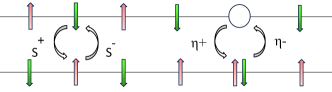
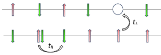
Different terms in the Hamiltonian have the following physical meanings: is the spin interaction term, familiar from the standard t-J model; is the -exchange term, which exchanges the position of a doublon and holon and causes the interaction between DH pair if they are on nearest neighbor sites; and represent hopping of holon and doublon conserving their number, respectively. These processes are illustrated in Fig. 1. In the sectors with no doublon quasi-particle, reduces to the standard t-J model. is the on-site Coulomb interaction and leads to unimportant energy shift between the chemical and photo-doped system. Both chemically and photo-doped systems reduce to the solution of the ground state problem in different sectors and we employ the exact diagonalization using the Lanczos technique [57, 58].
We should note that in the full expansion there appear also three site terms which are of two types: a) the holon/doublon correlated hopping terms of order which conserve the number of holon and doublon pairs and the analysis in Ref. 47 showed that their effect is small in the dilute limit considered here, b) recombination terms of order which we will for a moment suppress to mimic the metastable state by an equilibrium problem. Later on, we will estimate the lifetime of the metastable phase (recombination time) by perturbative treatment of these 3-site recombination terms.
III Results for two-leg ladder
Our aim is to study the properties of bound doublon-holon (Hubbard excitons) or two holon states and compare the binding of charged carriers in photo and chemically doped situation. An important goal is to understand the interplay of spin and fluctuations on the doublon-holon binding, in systems beyond one dimension, which is special due to the spin-charge and spin--charge separation [47, 54].
We start our analysis with the simplest system which escapes the separation, namely the two-leg ladder system, and later extend the study to the two-dimensional situation.
III.1 Exciton binding energy
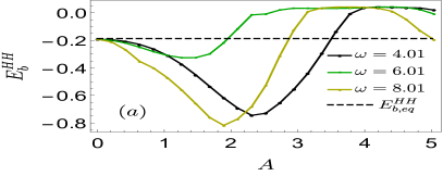
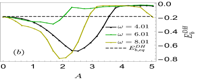
The tendency towards binding between charged particles can be quantified by the binding energy [8, 59, 43, 38], which for the chemically doped state is expresses as and for the photo-doped states by , where refer to the ground state energy of in the sector with two holons, one doublon-holon pair, one holon, one doublon, and only singly occupied sites, respectively. The criterion for the formation of a bound pair is a negative binding energy, . In all of the results below, we will measure the binding energy in the units of . We should stress that the analysis below suffers from a particular finite size effect: while are energies of ground states at zero momentum, ground state for the sector with a single holon/doublon appear at a finite momentum , which might not be present for a given system size . In any case, we use the solution with lowest energy. To validate the robustness of our conclusion despite finite size difficulties, we will further compare the binding energy with real-space correlators to support the binding.
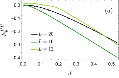
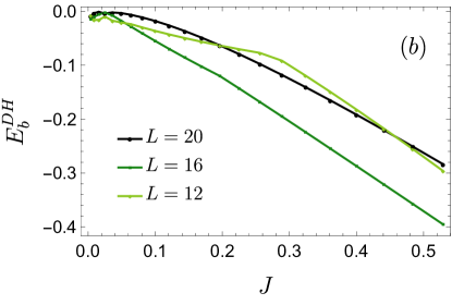
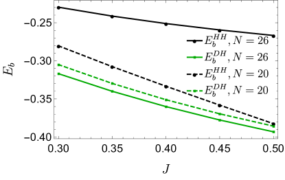
We start the analysis with the isotropic case () and show that a finite binding is present for a large parameter regime, , and it increases as a function of superexchange coupling, see Fig. 2. At large , the magnitude of binding between a DH pair and two holons become identical, while for small values of the binding energies for the two kinds of exciton differ; however the difference is getting smaller with increasing system size. The increased binding in the limit of large superexchange comes from the fact that the breaking of spin and fluctuations is more and more energetically penalized, leading to localization of the charged pair.
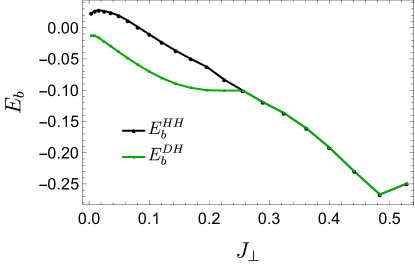
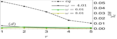
Recent theoretical and experimental studies on binding of two holons showed that by using external electic field [28, 27] one can create highly anisotropic superexhange couplings, which can be favourable for binding. Here, we would like to explore this perspective by tuning the anisotropy to understand which parameter regime is favourable for both type of bindings. Fig. 3 shows the binding energy as a function of , keeping the parallel exchange parameter fixed . Initially, binding energy grows with increasing , but then the trend is reversed due to the competition of charge delocalization, promoted by the increase in , and localization aided by large . This suggests that ideally, we would like to decouple and to increase only the latter. In Section III.3, we will elucidate the methodology employed to accomplish this objective through Floquet engineering. As a side note, we notice that the binding energy for the two different charged pairs becomes equal for .
Comparable binding energy for chemically and photo-doped systems means there is no clear competition or cooperation for binding due to spin and fluctuations. We consider this as the first important message of this paper. An useful starting point to understand the observation is to analyze the ground state of a 22 cluster for the anisotropic case, , such that the DH or HH pairs are present in the same rung to reduce the energy lost by the breaking of the spin bonds [8, 59]. The ground state manifold for two holons consists of two states, and , where the top row represent the spin configuration in the upper chain and bottom in the lower chain. The ground state energy of this manifold is . For the case of one DH pair, we work in the manifold with four states, , , and . The ground state energy of this manifold is . Notice that the binding energies and become identical only when we consider the -exchange terms between the doublon and holon. This outlines the importance of this term for the analysis of Hubbard excitons [47, 53]. To obtain analytical estimations, we have neglected the hopping terms, which crucially differ between holon and doublons as well. While holon (as a quasiparticle) has a negative hopping sign, doublon has a positive one since by moving a doublon we always hop over one fermion. At least in 2D systems, this can crucially influence the symmetry of the bound states, as pointed out in Refs. 43, 38, 60.
III.2 Charge and spin correlators
An alternative way to characterize the properties of bound states are real space correlators. The charge correlators determine the relative spatial distribution of charged carriers. For the DH and HH pair, they are defined as and , respectively. Furthermore, to capture the relative alignment of the up and down spins we define the spin correlator .
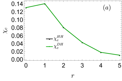
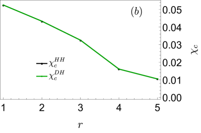
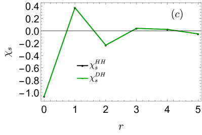
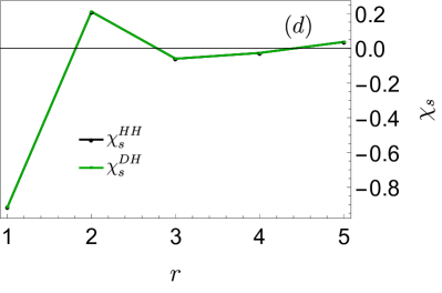
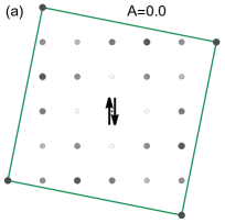
We show the charge correlator (top) and spin correlator (bottom) between the chains (left) and along the chain (right) in Fig. 4. For the isotropic case shown, not only the binding energies , c.f. Fig. 3, but also the correlators are indistinguishable for the DH and HH pairs. Exponentially decaying charge correlations for charges positioned in different legs, Fig. 4(a) are in agreement with the state being bound. It is worth noting that the binding along the same leg is considerably weaker, Fig. 4(b). The spin correlator, Fig. 4(c,d), confirms anti-ferromagnetic local fluctuations, which mediate the binding. While hopping terms tend to delocalise the charged pair, this causes a disturbance in the antiferromagnetic spin pattern. The competition between the two processes yields the existence of non-trivial bound states, with, for example, the strongest occupation of charged particles along the diagonal and not along the rung bond, as would be the case in the absence of hopping terms [61]. For the DH pair, we have also evaluated the real-space superconducting correlator (not shown), which shows a staggered long-range correlations characteristic for -pairing state and consistent with recent time-dependent DMRG study [48].
III.3 Enhanced Binding by Floquet Drive
Increasing the exchange coupling by reducing the interaction is one way to achieve the enhanced binding (Fig. 2), however, this approach has limitations since we must remain in the perturbative regime . Alternatively, tuning the rung hopping , resulting in the anisotropy , in some cases leads toenhanced binding energy as well (Fig. 3), however, the enhancement is limited by the increase in which tend to delocalize the charges. Here we would like to explore whether manipulating the hopping and the exchange coupling independently could even further increase the stability of bounds states. Previously, this was achieved by introducing a potential term in one of the rungs [27]. We further harness this idea by introducing a time-periodic field and explore the Floquet engineering of the effective model to enhance the stability of bounds states.
We drive the system with an external electric field applied along the rung and introduced via Peierls substitution to the hopping term, , between nearest neighbor sites and . Here, is the equilibrium rung hopping parameter, is the vector potential and is the vector from to the site. The charge of the particles and distance between nearest neighbours is considered unity; hence the electric field is related to the vector potential by . For field in the direction of the rung , the hopping and exchange couplings along the chain (, ) remain the same as in the equilibrium. Let us write the interaction strength as , where is the closest approximation to in multiples of and act as the detuning. The Fourier components are then expressed as,
| (4) |
where is the Bessel function of order . Here, we have used the relation .
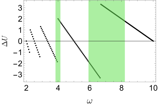
Depending on the value of there are different regimes; far-from-resonant driving with and near-resonant driving with , which can be treated with appropriate high-frequency expansions [30, 29, 31, 62]. We will consider only the off-resonant driving, in Fig. 5 denoted by the green regions, as heating and doublon-holon recombination effects are suppressed in this regime, see Sec V.
After performing the high-frequency expansion in the off-resonant regime and neglecting higher order terms, see App. A, we arrive at the effective Floquet Hamiltonian of form (II), where parameters along the chains equal to the equilibrium ones, while both hopping and exchange parameters in the rung (field) direction depend on the drive parameters and get modified as [30, 29, 31, 62]
| (5) | |||||
| (6) | |||||
| (7) |
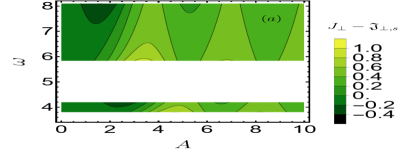
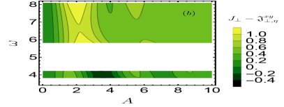
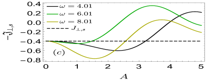
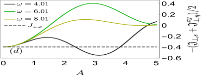
Applying a periodic drive thus gives the freedom to vary hopping and different exchange parameters independently. In Fig. 6, we show the variation of (a) and (b) as a function of the field strength and frequency . White regions in the plot correspond to areas that do not obey the limit, . Regions with (stronger than equilibrium spin exchange coupling) and (stronger than equilibrium pairing exchange coupling) are candidate regions in which enhanced exchange couplings could mediate stronger binding between the charged particles.
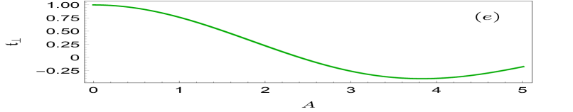
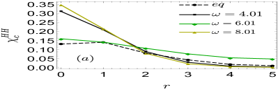
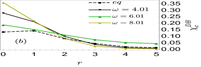
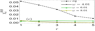
Now, we will check how well such predictions work by analyzing the binding energy of charge carriers within the effective Floquet Hamiltonian . We will focus on the field amplitude dependence at three frequencies, . Figs. 7(a,b) shows the binding energy for the HH and DH pair, respectively. In Figs. 7(b,c) we show for comparison the binding energy estimates extracted from the 22 clusters, for an HH pair given by and for a DH pair given by . Indeed, the binding energy for HH pair is increased in the similar range where also spin exchange coupling is increased compared to the equilibrium value. Comparison of the DH binding energy (Fig 7(b)) with its cluster estimate (Fig 7(d)) shows that the DH binding is enhanced in a broader range of the excitation strengths than anticipated from the 2x2 cluster estimation. We attribute the difference to the fact that the hopping strength is substantially reduced in this regime of (Fig. 7(e)), which should be favourable for binding. Overall, the conclusion is that the Floquet driving leads to a substantial modification of the pair binding energies, which can be enhanced to more than three times compared to the equilibrium values.
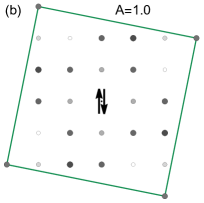
To further ensure that the enhanced binding energies indeed lead to a more bound pair we consider real-space HH and DH correlators. In Fig. 8, we compare the charge correlators for the system under the Floquet drive to its equilibrium counterpart. The inter-chain correlators show that in the regions of the enhanced bindings (e.g. A=1.98), the charge carriers are indeed residing at substantially closer distances both for HH and DH pair, see Fig. 8(a) and (b). Furthermore, the intra-chain correlators shows a strong reduction with respect to the equilibrium value, which means that the two charge carriers will tend to form pairs in the opposite chain along the rung. These results show that the Floquet driving can substantially increase the tendency of charge carriers to form bound pairs.
Based on the above analysis, we find that Floquet engineering can result in significantly enhanced binding energies due to the reduction of the hopping integral and the enhancement of spin and fluctuations. At least in the two-leg ladder system, enhancing HH binding appears in a broader regime of drive parameters since it only requires increased . To increase DH binding, we preferentially want to increase both and , which seems to be exclusive in many cases. However, the enhanced DH binding is still present in a broad parameter regime as the Floquet driving decreases the effective hopping integral, leading to a higher tendency for excitonic bindings.
Now, we analyze how these findings are translated to 2D systems.
IV Results for two dimensional square lattice
We will consider 2D lattices with periodic boundary conditions for which the and direction are equivalent; therefore, the and terms in the effective model , Eq. (II), are equivalent. At least in equilibrium, i.e., without any Floquet engineering, all the exchange couplings are the same and equal .
The question of HH and DH binding in 2D has already been addressed theoretically [43, 63, 38, 64, 60, 11, 8], as of relevance for the high-temperature superconductivity in effectively two dimensional doped cuprates [8] and photo-doped charge transfer and Mott insulating materials [65, 66, 44, 67]. It has been recently experimentally confirmed that in photo-doped charge transfer and Mott insulating materials, bound states of doublon-holon pairs, i.e., Hubbard excitons, indeed appear as metastable states that form after the pump pulse. They can be detected via a transfer of spectral weight from the Drude peak to a finite frequency Lorenzian [67] and in the third order optical response [44]. Another indirect clue for the presence of doublon-holon excitons comes from an exponential functional form of the mid-infrared peak decay in photo-doped materials [65, 66, 68], reflecting that the recombination process of doublon-holon pair happens from a bound state. The recombination rate is exponentially suppressed in the number of bosonic excitations that are emitted in the process, in order to bridge the Mott gap [38, 64]. Furthermore, it was shown that the non-local Coulomb interaction can cooperate with the super-exchange coupling assisted excitons formation [38, 39, 67].
Here we revisit the equilibrium analysis and compare the HH and DH binding. As opposed to the previous studies of DH Hubbard excitons, we include here the effect of fluctuations, by keeping the term in the effective Hamiltonian , Eq. (II), that we diagonalize using Krylov technique in the sector with one holon-holon and one doublon-holon pair on system of size up to sites.
IV.1 Equilibrium results
In Fig. 9, we show binding energies for holon-holon and doublon-holon pair as a function of on systems of size sites. To minimize the finite size effects on lattices that do not have the wave vector (which is the case for ), we use for and the fit obtained from in Ref. 69. As in the two-leg ladder, increasing the exchange coupling enhances the binding energy, since breaking the short-range antiferromagnetic spin fluctuations is energetically penalized, leading to localization of the pair. Our results suggest that in 2D, including the term slightly reduces the binding energy of DH exciton, which suggests that fluctuations do not help to stabilize the exciton. However, the contribution is not very significant so the Hubbard excitons are stable even if this term is taken into account. Unlike in the two-leg ladder setup, here, doublon-holon and holon-holon binding energies are always distinct, and this is true with or without including the fluctuations. We hypothesise that this can be traced back to the difference in phases in the hopping term for holon and doublon, Eq. (II), which is known to result in different wave function symmetry of the two bound states: while the holon-holon bound states has -wave symmetry, the doublon-holon bound states has -wave symmetry [43]. As some of us recently discussed in relation to experimental observation of intra-excitonic transitions [67], there actually exist several DH Hubbard excitons with different symmetries. Here, however, we discuss only the lowest and most stable one.
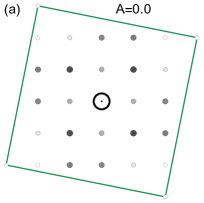
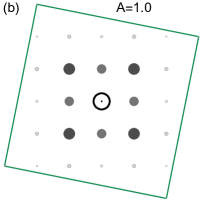
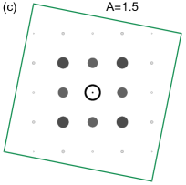
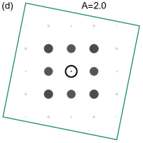
In Fig. 10(a), we plot the charge correlator , showing the distribution of holon relative to the doublon (in the origin) for the Hubbard exciton state at . Results are in agreement with a bound state, however, we can see that the excitonic state is rather extended: the largest contribution to the excitonic wave function comes from holon and doublon being only the third nearest neighbors. In Fig. 11(a), we plot an equivalent charge correlator for the holon-holon bound state, showing the distribution of one holon (in the origin) relative to the other one for . Results are again in agreement with a bound state.
IV.2 Floquet engineering
Lastly, we revisit the Floquet engineering of exchange coupling parameters from Sec. III.3. In the two-leg ladder, we considered the electric field along the rung with which modulated only the exchange coupling along the rungs. Here, we consider the electric field applied along the diagonal, with . Then, the four-fold symmetry of the 2D lattice is preserved and exchange coupling between all the nearest neighbors are the same. We will again present results for the off-resonant regime with , where different exchange terms are given by Eq. (6) and Eq. (7).
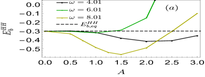
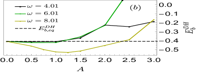
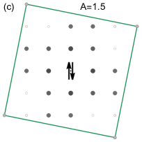
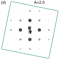
In Fig. 12, we show the variation of the binding energy for holon-holon and doublon-holon pair as a function of for and . We choose the same frequencies as in the corresponding study in the two-leg ladder. In this case, we use for the energies at the momentum with lowest g.s. energy for the given system size; the values of effective exchange parameters vs. the hopping are outside of the validity of fit from Ref. 69 used in the static case. Like in the ladder geometry, there is an extended regime of field strengths for which the binding is enhanced via the Floquet engineering of coupling parameters. This conclusion is supported also by the DH and HH correlators, which are in Fig. 10(b,c,d) and Fig. 11(b,c,d) shown for field strengths . It is clearly visible that for a region of parameters , the DH and HH pairs get more localized than at equilibrium. In the extreme case of large driving, e.g. for DH pair in Fig. 10, the DH pair resides at the nearest-neighbor sites in stark contrast to the equilibrium value.
This result once again underlines that Floquet engineering is indeed a relevant approach that can significantly increase the localization of the bound states and should be a viable option that could be implemented in either solid state or cold atoms setups. For the latter, we draft our suggestion in Section VI.
V Recombination of Hubbard excitons
While Floquet driving can increase the binding of charged pairs by modifying the effective hopping and exchange parameters, it also has an influence on the doublon-holon recombination rate that determines the timescale on which excitons are stable and observable. Namely, Floquet driving opens additional recombination channels and therefore it is important to understand how stable is the excitonic state in the driven case.
Due to the large energy of the Mott gap that must be instantaneously released in the recombination process of a doublon-holon pair, the recombination timescale is much slower than the timescale for the intrinsic dynamics/relaxation of holons and doublons within each Hubbard band. Even though recombination appears in the Hubbard model within the hopping term of strength , it is reasonable to treat it perturbatively: we have made this formal in Sec. II by canonically transforming the original model, Eq. (II), so that recombination term appears with a smaller prefactor (e.g., ) in the transformed one. Transformation yields the effective Hamiltonian , Eq. (II), that preserves the number of doublon-holon pairs, using which we can elegantly estimate the metastable excitonic state. Moreover, the transformation also singles out the dominant recombination, now with a prefactor of the order [70, 38],
| (8) |
where is spin opposite to and are nearest-neighbor sites to . In the static setup and at a low density of photoexcited DH pairs, the only viable recombination channel is via emission of spin excitations, which absorb the large energy of the Mott gap as doublon and holon recombine across the gap. The recombination rate can be numerically estimated via Fermi’s golden rule expression for the transition from the excitonic state into a highly excited state of spins with energy ,
| (9) |
In Refs. 70, 64, some of us showed that the recombination rate is roughy exponentially suppressed in the number of spin excitation that are emitted in such a process. A more precise dependence on the model parameters was derived in Ref. 71 by making a connection to the exciton-boson model, where exciton recombines by emitting some general boson excitations. In this case the decay rate can be approximated by
| (10) |
where is the prefactor in the operator causing the recombination, is the dimensionless coupling strength between the exciton and bosons, and is the typical energy of bosons emitted. For coupling to spins, , was fitted to be roughly , and was fitted to , corresponding to the actual prefactor in , Eq. (8).
In the case of Floquet driving with the original time-dependent Hubbard model, a strategy to estimate the recombination rate is to perform a time-dependent canonical transformation, which once again transforms out the recombination term (from the time-dependent model) at order . Inspired by Ref. 72, we perform this transformation in App. B and obtain that in the lowest order of the high-frequency expansion, the dominant recombination term has the same structure as in the static case, but with a different prefactor,
| (11) |
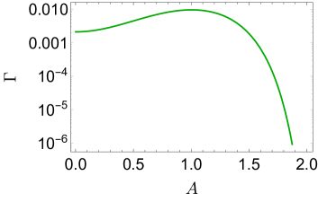
Most importantly, the recombination term tells us that Floquet driving opens additional recombination channels in which magnons and photons can be emitted subsequently: emission of photons is suppressed by factor, but it implies that a considerably smaller energy must be received by spin excitations. Potentially, this can drastically shorten the recombination time and the stability of the exciton. However, such formalism can not capture a process where interference between the photon and the magnon emission would be considered. Currently, we do not know how to treat such a process fully and we will provide an upper bound for the recombination time assuming independent photon/magnon emission. Since the form of the recombination operator is the same in the static and Floquet case, we estimate the recombination rate by expression (10). In the Floquet case, we use , where is the floor function, as the minimal energy that must be emitted into spin excitations, as a typical renormalized magnon energy, and . For expression (10) to be valid, , which is not the case for every choice of Floquet parameters. In addition, we should stress that this approach does not correctly reproduce the recombination rate for the limit, when the full Mott gap energy should be absorbed by the spins. Nonetheless, we show in Fig. 13 this rather pessimistic upper bound estimate of the recombination rate dependence on the field strength for , in which case (10) is in the valid regime. We anticipate that this result strongly overestimates the recombination rate at small field strengths . But it does also tell as that for such a driving, the binding energy is always at least an order larger then the width of the excitonic peak. While our study is by no means conclusive, it open the question of better estimating the bound state’s lifetime in all regimes, but most importantly in the regime where Floquet driving most significantly enhances binding.
While holon-holon bound states do not suffer from recombination, the opposite process of doublon-holon creation would plague the stability of HH binding in the Floquet setup at the same rate .
VI Photo-doped states in cold atoms experiments
While the existence of the doublon-holon excitons has been primarily discussed in the context of photo-doped solid-state setups [73, 74, 75, 76, 77], cold-atom experiments could serve as an excellent testbed to study properties of photo-doped states. Recently, there has been tremendous progress in understanding half-filled [21] and doped Fermi-Hubbard systems with cold atom setups [78] exhibiting paradigmatic non-perturbative effects such as the pseudogap [79], spin strings [80, 23], linear resistivity [81], etc. The application of the Floquet engineering to the chemically doped systems presented in this work can be straightforwardly extended to cold atom setups. A new avenue is the extension to photo-doped systems and we propose simple protocols enabling a systematic study of differences between the chemically and photo-doped phase diagrams. We will consider two protocols to prepare the photo-doped state: the adiabatic state preparation from band to Mott insulator and (chirped) excitation across the Mott gap.
Adiabatic state preparation
In the first protocol, we start from a Mott-insulating state, where two sites have large positive and negative on-site potential, leading to fully occupied and empty states. Now, one can slowly reduce the on-site potential, allowing for the virtual dressing of the empty and full state with charge and spin fluctuations. The ramp velocity has to be slow enough so that the Landau-Zenner tunnelling across the Mott gap is suppressed [82, 83, 70]. With this respect, it might be convenient to first prepare the doublon-holon pair at high values of the Mott repulsion and then reduce it to the desired value. Such protocols can be easily extended to multiple holon-doublon pairs. This would allow us to study a complete phase diagram of photo-doped Mott insulators, including peculiar long-range phases such as the -pairing superconductivity or the charge-density wave [47, 53].
Excitations accross the gap
A standard approach to create holon-doublon pair is to either excite the system with a resonant excitation or apply an electric field comparable to the Mott gap. A naive implementation of the protocol would lead to a highly excited state with broad distribution of holes and doublon within the Hubbard band [84] which is detrimental for the formation of Hubbard excitons with rather small binding energies and would require a substantial coupling with an external heat bath. Instead, we propose using a chirped pulse (either electromagnetic or parameter modulation) with the base frequency slightly below the Mott gap, which is then slowly chirped across the Mott gap. It was shown in Ref. [85, 86, 53, 86] that such a protocol creates a quasi-equilibrium distribution with low effective temperatures and doublon-holon excitons should emerge as a stable structure.
Upon the successful preparation of the doublon-holon state through either of the prescribed protocols, one can initiate the application of the proposed Floquet engineering technique (Eq. (III.3)) to manipulate the exciton binding energy. Analogous superexchange manipulation can be obtained by directly modifying hopping [32].
VII Conclusions
In this work, we compared the pairing of chemically and photo-doped charge carriers mediated by spin and fluctuations in ladder and 2D systems. As the photo-doped state is metastable, we employed the Schrieffer-Wolf transformation to approximate the long-lived phase as a quasi-equilibrium state described by an extended t-J model. We establish that the binding is comparable in the two regimes by analysing binding energies and real-space correlators. In equilibrium and within the single-band Hubbard model, the superexchange and the hopping are connected and while the increase of the superexchange would enhance charge pairing it naturally comes with the increase of the hopping, leading to the tendency to delocalize charge carriers. We used Floquet engineering to decouple the two and the analysis yields an effective Floquet Hamiltonian, where both the superexchange and the hopping are modified by the driving frequency and the amplitude . We demonstrate that a judicious selection of drive parameters can substantially enhance the strength of binding between exciton pairs both for ladders and 2D systems, although the increase in the latter is limited in a narrower driving range. The tendency to form bound pairs is most obvious in the analysis of the real-space correlators, which show a dramatic reduction in the relative distance between pairs. Finally, we provided an upper bound on the lifetime of the metastable phase using a Fermi golden rule argument and commented on how our theoretical predictions could be analyzed in cold-atom experiments.
Our estimation of the lifetime provides only an upper and most probably pretty pessimistic limit for the lifetime of the holon-doublon pair. Extending the description, which would consider both possible interferences between photon and magnon-assisted recombination and properly capture the limit of weak driving, is an important future problem. One direction would be a simulation of the full Hubbard model prepared with a holon-doublon pair and the inclusion of periodic driving. An alternative approach is to generalize the Floquet Fermi golden rule [87] approach for photo-doped Mott insulators, where the number of holons and doublons present an almost conserved quantity.
In the current work, we have focused on a dilute limit with a single pair; however, the formation of long-ranged orders will depend on the interaction between bound pairs. An exciting new perspective is to understand what is the effective interaction between holon-doublon pairs and what would be the symmetry of the -paired condensate in the ladder and 2D systems. As the Floquet driving can change the pairing of bound pairs, it will also have an effect on the interaction between pairs and a systematic analysis of these processes is needed to understand how to stabilize non-thermal states with long-range orders.
Acknowledgements.
We thank Y. Murakami, T. Kaneko, M. Bukov, and M. Eckstein for several useful discussions. We acknowledge the support by the projects J1-2463, N1-0318, MN-0016-106 and P1-0044 program of the Slovenian Research Agency, the QuantERA grant T-NiSQ by MVZI, QuantERA II JTC 2021, and ERC StG 2022 project DrumS, Grant Agreement 101077265. ED calculations were performed at the cluster ‘spinon’ of JSI, Ljubljana.References
- Lee et al. [2006] P. A. Lee, N. Nagaosa, and X.-G. Wen, Rev. Mod. Phys. 78, 17 (2006).
- Warren et al. [1989] W. W. Warren, R. E. Walstedt, G. F. Brennert, R. J. Cava, R. Tycko, R. F. Bell, and G. Dabbagh, Phys. Rev. Lett. 62, 1193 (1989).
- Norman et al. [2005] M. R. Norman, D. Pines, and C. Kallin, Advances in Physics 54, 715 (2005).
- Wu et al. [2018] W. Wu, M. S. Scheurer, S. Chatterjee, S. Sachdev, A. Georges, and M. Ferrero, Phys. Rev. X 8, 021048 (2018).
- Tranquada et al. [1995] J. M. Tranquada, B. J. Sternlieb, J. D. Axe, Y. Nakamura, and S. Uchida, Nature 375, 561 (1995).
- Corboz et al. [2014] P. Corboz, T. M. Rice, and M. Troyer, Phys. Rev. Lett. 113, 046402 (2014).
- Wietek et al. [2021] A. Wietek, Y.-Y. He, S. R. White, A. Georges, and E. M. Stoudenmire, Phys. Rev. X 11, 031007 (2021).
- Dagotto [1994] E. Dagotto, Rev. Mod. Phys. 66, 763 (1994).
- Maier et al. [2006] T. A. Maier, M. S. Jarrell, and D. J. Scalapino, Phys. Rev. Lett. 96, 047005 (2006).
- Maier et al. [2008] T. A. Maier, D. Poilblanc, and D. J. Scalapino, Phys. Rev. Lett. 100, 237001 (2008).
- Jaklič and Prelovšek [2000] J. Jaklič and P. Prelovšek, Advances in Physics 49, 1 (2000).
- Trugman [1988] S. A. Trugman, Phys. Rev. B 37, 1597 (1988).
- Bonča et al. [1989] J. Bonča, P. Prelovšek, and I. Sega, Phys. Rev. B 39, 7074 (1989).
- Chernyshev et al. [1998] A. L. Chernyshev, P. W. Leung, and R. J. Gooding, Phys. Rev. B 58, 13594 (1998).
- Bonča et al. [2007] J. Bonča, S. Maekawa, and T. Tohyama, Phys. Rev. B 76, 035121 (2007).
- Ogata and Shiba [1990] M. Ogata and H. Shiba, Phys. Rev. B 41, 2326 (1990).
- SHIBA and OGATA [1991] H. SHIBA and M. OGATA, International Journal of Modern Physics B 05, 31 (1991).
- Giamarchi [2003] T. Giamarchi, Quantum physics in one dimension, Vol. 121 (Clarendon press, 2003).
- Essler et al. [2005] F. H. Essler, H. Frahm, F. Göhmann, A. Klümper, and V. E. Korepin, The one-dimensional Hubbard model (Cambridge University Press, 2005).
- Dagotto et al. [1992] E. Dagotto, J. Riera, and D. Scalapino, Phys. Rev. B 45, 5744 (1992).
- Mazurenko et al. [2017] A. Mazurenko, C. S. Chiu, G. Ji, M. F. Parsons, M. Kanász-Nagy, R. Schmidt, F. Grusdt, E. Demler, D. Greif, and M. Greiner, Nature 545, 462 (2017).
- Koepsell et al. [2019] J. Koepsell, J. Vijayan, P. Sompet, F. Grusdt, T. A. Hilker, E. Demler, G. Salomon, I. Bloch, and C. Gross, Nature 572, 358 (2019).
- Chiu et al. [2019] C. S. Chiu, G. Ji, A. Bohrdt, M. Xu, M. Knap, E. Demler, F. Grusdt, M. Greiner, and D. Greif, Science 365, 251 (2019), https://www.science.org/doi/pdf/10.1126/science.aav3587 .
- Bohrdt et al. [2019] A. Bohrdt, C. S. Chiu, G. Ji, M. Xu, D. Greif, M. Greiner, E. Demler, F. Grusdt, and M. Knap, Nature Physics 15, 921 (2019).
- Trotzky et al. [2008] S. Trotzky, P. Cheinet, S. Fölling, M. Feld, U. Schnorrberger, A. M. Rey, A. Polkovnikov, E. A. Demler, M. D. Lukin, and I. Bloch, Science 319, 295 (2008), https://www.science.org/doi/pdf/10.1126/science.1150841 .
- Dimitrova et al. [2020] I. Dimitrova, N. Jepsen, A. Buyskikh, A. Venegas-Gomez, J. Amato-Grill, A. Daley, and W. Ketterle, Phys. Rev. Lett. 124, 043204 (2020).
- Hirthe et al. [2023] S. Hirthe, T. Chalopin, D. Bourgund, P. Bojović, A. Bohrdt, E. Demler, F. Grusdt, I. Bloch, and T. A. Hilker, Nature 613, 463 (2023).
- Bohrdt et al. [2022] A. Bohrdt, L. Homeier, I. Bloch, E. Demler, and F. Grusdt, Nature Physics 18, 651 (2022).
- Bukov et al. [2015] M. Bukov, L. D’Alessio, and A. Polkovnikov, Advances in Physics 64, 139 (2015), https://doi.org/10.1080/00018732.2015.1055918 .
- Bukov et al. [2016] M. Bukov, M. Kolodrubetz, and A. Polkovnikov, Phys. Rev. Lett. 116, 125301 (2016).
- Mentink et al. [2015] J. H. Mentink, K. Balzer, and M. Eckstein, Nature Communications 6, 6708 (2015).
- Görg et al. [2018] F. Görg, M. Messer, K. Sandholzer, G. Jotzu, R. Desbuquois, and T. Esslinger, Nature 553, 481 (2018).
- Murakami et al. [2023a] Y. Murakami, D. Golež, M. Eckstein, and P. Werner, Photo-induced nonequilibrium states in mott insulators (2023a), arXiv:2310.05201 [cond-mat.str-el] .
- de la Torre et al. [2021] A. de la Torre, D. M. Kennes, M. Claassen, S. Gerber, J. W. McIver, and M. A. Sentef, Rev. Mod. Phys. 93, 041002 (2021).
- Sensarma et al. [2010] R. Sensarma, D. Pekker, E. Altman, E. Demler, N. Strohmaier, D. Greif, R. Jördens, L. Tarruell, H. Moritz, and T. Esslinger, Phys. Rev. B 82, 224302 (2010).
- Strohmaier et al. [2010] N. Strohmaier, D. Greif, R. Jördens, L. Tarruell, H. Moritz, T. Esslinger, R. Sensarma, D. Pekker, E. Altman, and E. Demler, Phys. Rev. Lett. 104, 080401 (2010).
- Kollath et al. [2007] C. Kollath, A. M. Läuchli, and E. Altman, Phys. Rev. Lett. 98, 180601 (2007).
- Lenarčič and Prelovšek [2013] Z. Lenarčič and P. Prelovšek, Phys. Rev. Lett. 111, 016401 (2013).
- Bittner et al. [2020] N. Bittner, D. Golež, M. Eckstein, and P. Werner, Phys. Rev. B 101, 085127 (2020).
- Sugimoto and Ejima [2023] K. Sugimoto and S. Ejima, Pump-probe spectroscopy of the one-dimensional extended hubbard model at half filling (2023), arXiv:2305.09909 [cond-mat.str-el] .
- Jeckelmann [2003] E. Jeckelmann, Phys. Rev. B 67, 075106 (2003).
- Matsueda et al. [2004] H. Matsueda, T. Tohyama, and S. Maekawa, Phys. Rev. B 70, 033102 (2004).
- Tohyama [2006] T. Tohyama, Journal of the Physical Society of Japan 75, 034713 (2006).
- Terashige et al. [2019] T. Terashige, T. Ono, T. Miyamoto, T. Morimoto, H. Yamakawa, N. Kida, T. Ito, T. Sasagawa, T. Tohyama, and H. Okamoto, Science Advances 5, eaav2187 (2019), https://www.science.org/doi/pdf/10.1126/sciadv.aav2187 .
- Rosch et al. [2008] A. Rosch, D. Rasch, B. Binz, and M. Vojta, Phys. Rev. Lett. 101, 265301 (2008).
- Kaneko et al. [2019] T. Kaneko, T. Shirakawa, S. Sorella, and S. Yunoki, Phys. Rev. Lett. 122, 077002 (2019).
- Murakami et al. [2022] Y. Murakami, S. Takayoshi, T. Kaneko, Z. Sun, D. Golež, A. J. Millis, and P. Werner, Communications Physics 5, 23 (2022).
- Ueda et al. [2023] R. Ueda, K. Kuroki, and T. Kaneko, Photoinduced -pairing correlation in the hubbard ladder (2023), arXiv:2310.10153 [cond-mat.str-el] .
- Kaneko et al. [2020] T. Kaneko, S. Yunoki, and A. J. Millis, Phys. Rev. Res. 2, 032027 (2020).
- Ejima et al. [2020] S. Ejima, T. Kaneko, F. Lange, S. Yunoki, and H. Fehske, Phys. Rev. Res. 2, 032008 (2020).
- Tindall et al. [2019] J. Tindall, B. Buča, J. R. Coulthard, and D. Jaksch, Phys. Rev. Lett. 123, 030603 (2019).
- Shirakawa et al. [2020] T. Shirakawa, S. Miyakoshi, and S. Yunoki, Phys. Rev. B 101, 174307 (2020).
- Li et al. [2020] J. Li, D. Golez, P. Werner, and M. Eckstein, Phys. Rev. B 102, 165136 (2020).
- Murakami et al. [2023b] Y. Murakami, S. Takayoshi, T. Kaneko, A. M. Läuchli, and P. Werner, Phys. Rev. Lett. 130, 106501 (2023b).
- Eckstein and Werner [2011] M. Eckstein and P. Werner, Phys. Rev. B 84, 035122 (2011).
- MacDonald et al. [1988] A. H. MacDonald, S. M. Girvin, and D. Yoshioka, Phys. Rev. B 37, 9753 (1988).
- Prelovšek and Bonča [2013] P. Prelovšek and J. Bonča, in Springer Series in Solid-State Sciences (Springer Berlin Heidelberg, 2013) pp. 1–30.
- Lanczos [1950] C. Lanczos, Journal of Research of the National Bureau of Standards 45, 255 (1950).
- Troyer et al. [1996] M. Troyer, H. Tsunetsugu, and T. M. Rice, Phys. Rev. B 53, 251 (1996).
- Shinjo et al. [2021] K. Shinjo, S. Sota, and T. Tohyama, Phys. Rev. B 103, 035141 (2021).
- White and Scalapino [1997] S. R. White and D. J. Scalapino, Phys. Rev. B 55, 6504 (1997).
- Murakami et al. [2023c] Y. Murakami, M. Schüler, R. Arita, and P. Werner, Phys. Rev. B 108, 035151 (2023c).
- Takahashi et al. [2002] M. Takahashi, T. Tohyama, and S. Maekawa, Phys. Rev. B 66, 125102 (2002).
- Lenarčič and Prelovšek [2014] Z. Lenarčič and P. Prelovšek, Phys. Rev. B 90, 235136 (2014).
- Okamoto et al. [2010] H. Okamoto, T. Miyagoe, K. Kobayashi, H. Uemura, H. Nishioka, H. Matsuzaki, A. Sawa, and Y. Tokura, Phys. Rev. B 82, 060513 (2010).
- Okamoto et al. [2011] H. Okamoto, T. Miyagoe, K. Kobayashi, H. Uemura, H. Nishioka, H. Matsuzaki, A. Sawa, and Y. Tokura, Phys. Rev. B 83, 125102 (2011).
- Mehio et al. [2023] O. Mehio, X. Li, H. Ning, Z. Lenarčič, Y. Han, M. Buchhold, Z. Porter, N. J. Laurita, S. D. Wilson, and D. Hsieh, Nature Physics , 1 (2023).
- Sahota et al. [2019] D. G. Sahota, R. Liang, M. Dion, P. Fournier, H. A. Dąbkowska, G. M. Luke, and J. S. Dodge, Phys. Rev. Res. 1, 033214 (2019).
- Leung and Gooding [1995] P. W. Leung and R. J. Gooding, Phys. Rev. B 52, R15711 (1995).
- Lenarčič and Prelovšek [2012] Z. Lenarčič and P. Prelovšek, Phys. Rev. Lett. 108, 196401 (2012).
- Karakonstantakis et al. [2011] G. Karakonstantakis, E. Berg, S. R. White, and S. A. Kivelson, Phys. Rev. B 83, 054508 (2011).
- Kitamura et al. [2017] S. Kitamura, T. Oka, and H. Aoki, Phys. Rev. B 96, 014406 (2017).
- Kishida et al. [2001] H. Kishida, M. Ono, K. Miura, H. Okamoto, M. Izumi, T. Manako, M. Kawasaki, Y. Taguchi, Y. Tokura, T. Tohyama, K. Tsutsui, and S. Maekawa, Phys. Rev. Lett. 87, 177401 (2001).
- Ono et al. [2004] M. Ono, K. Miura, A. Maeda, H. Matsuzaki, H. Kishida, Y. Taguchi, Y. Tokura, M. Yamashita, and H. Okamoto, Phys. Rev. B 70, 085101 (2004).
- Lu et al. [2015] H. Lu, C. Shao, J. Bonča, D. Manske, and T. Tohyama, Phys. Rev. B 91, 245117 (2015).
- Novelli et al. [2012] F. Novelli, D. Fausti, J. Reul, F. Cilento, P. H. M. van Loosdrecht, A. A. Nugroho, T. T. M. Palstra, M. Grüninger, and F. Parmigiani, Phys. Rev. B 86, 165135 (2012).
- Rincón and Feiguin [2021] J. Rincón and A. E. Feiguin, Phys. Rev. B 104, 085122 (2021).
- Bohrdt et al. [2021] A. Bohrdt, L. Homeier, C. Reinmoser, E. Demler, and F. Grusdt, Annals of Physics 435, 168651 (2021).
- Brown et al. [2020] P. T. Brown, E. Guardado-Sanchez, B. M. Spar, E. W. Huang, T. P. Devereaux, and W. S. Bakr, Nature Physics 16, 26 (2020).
- Xu et al. [2023] M. Xu, L. H. Kendrick, A. Kale, Y. Gang, G. Ji, R. T. Scalettar, M. Lebrat, and M. Greiner, Nature , 1 (2023).
- Brown et al. [2019] P. T. Brown, D. Mitra, E. Guardado-Sanchez, R. Nourafkan, A. Reymbaut, C.-D. Hébert, S. Bergeron, A.-M. S. Tremblay, J. Kokalj, D. A. Huse, P. Schauß, and W. S. Bakr, Science 363, 379 (2019), https://www.science.org/doi/pdf/10.1126/science.aat4134 .
- Oka and Aoki [2005] T. Oka and H. Aoki, Phys. Rev. Lett. 95, 137601 (2005).
- Oka and Aoki [2010] T. Oka and H. Aoki, Phys. Rev. B 81, 033103 (2010).
- Oka [2012] T. Oka, Phys. Rev. B 86, 075148 (2012).
- Werner et al. [2019a] P. Werner, M. Eckstein, M. Müller, and G. Refael, Nature Communications 10, 5556 (2019a).
- Werner et al. [2019b] P. Werner, J. Li, D. Golež, and M. Eckstein, Phys. Rev. B 100, 155130 (2019b).
- Ikeda and Polkovnikov [2021] T. N. Ikeda and A. Polkovnikov, Phys. Rev. B 104, 134308 (2021).
Appendix A Effective hamiltonian for the off-resonant regime
Here, we show the various steps involved in arriving at the effective Hamiltonian with the parameters shown in Eqs. (5-7). In the off-resonant regime, we first apply a unitary transformation by . The resultant Hamiltonian in the rotated frame is given by ). can be written as a sum of terms that preserve the number of DH pairs (), increase or decrease the DH pair number by one (, ).
| (12) |
Introducing, and , the various terms in can be written as
| (13) |
Using and Eq. (13) in Eq. (12),
| (14) | ||||
Notice that has two defining frequencies, U and . To make periodic in both U and we define a common frequency , such that and , where and are co-prime numbers. To calculate the effective Floquet Hamiltonian we do a high-frequency expansion of by expanding it with respect to different orders of the period . The first term in the expansion has the form [30],
Now using Eq. (14) in Eq. (A), the terms of the effective Floquet Hamiltonian at zeroth order are,
| (16) |
| (17) |
Since and are co-prime numbers, , and the above integral is zero. Similarly for the complex conjugate part . Hence, at the zeroth order in the high-frequency expansion the effective Hamiltonian is,
| (18) |
The next order term is given by
| (19) |
where is understood periodic with a period The first term is given by
| (20) |
since all the commutators vanish. The second term is given by
| (21) |
which rewritten in the frequency domain is,
| (22) |
is non-zero only when , and is non-zero only when . This gives, or , which is never satisfied since and are co-primes. As a result, and is never simultaneously non-zero and always. Similarly, the complex conjugate .
Appendix B Dominant recombination term in Floquet driven setup
To establish an approximate recombination rate in the Floquet driven setup with the help of the static expression, Eq. (10), we perform a different time dependent canonical transformation which, similar to the static case, transforms out recombination term in the lowest order but retains it in the next order.
Starting from the original Hamiltonian
| (25) |
where we again split the hopping term into contributions that either retain, increase or decrease the number of DH pairs, and define as the double occupancy operator.
Following Ref. 72 we introduce a time-dependent canonical transformation , and obtain the transformed Hamiltonian as,
| (26) |
is chosen to eliminate the terms off-diagonal in . To determine and order by order we expand them in powers of as, and . We can re-write Eq. (26) as
| (27) |
We truncate , since our aim is to keep recombination term in the second order and compare with the equilibrium analysis to get an upper bound for the recombination rate in the Floquet driven scenario. From Eq. (27),
| (28) |
we find that , which gives , i.e., it eliminates the recombination in the lowest order.
From Eq. (27) using , we get
| (29) |
The relevant term in the commutator causing the recombination is given by
| (30) |
The effect of this term in the lowest order of the high-frequency expansion is given by its time average over one time period,
| (31) |
We can explicitly write down using , defined in Appendix A as
| (32) |
Then by using Eq. (31), we find that the recombination Hamiltonian is given by,
| (33) |