Optimized measurements of chaotic dynamical systems via the information bottleneck

Abstract

Deterministic chaos permits a precise notion of a “perfect measurement” as one that, when obtained repeatedly, captures all of the information created by the system’s evolution with minimal redundancy. Finding an optimal measurement is challenging, and has generally required intimate knowledge of the dynamics in the few cases where it has been done. We establish an equivalence between a perfect measurement and a variant of the information bottleneck. As a consequence, we can employ machine learning to optimize measurement processes that efficiently extract information from trajectory data. We obtain approximately optimal measurements for multiple chaotic maps and lay the necessary groundwork for efficient information extraction from general time series.

Encapsulated in deterministic chaos is the fundamental obstruction to predictability that can result from nonlinearity in a system’s evolution, even in the absence of randomness [shaw1981, eckmannruelle1985]. Signatures of chaos are found broadly, from weather [tsonis1989chaosweather, slingo2011weatheruncertainty] to the brain [kargarnovin2023evidence, skinner1992application], and tools developed in the study of chaos have been applied more broadly still [nicolis2012foundations, bradley2015nonlinear]. Advancing capabilities to forecast chaotic dynamics thus has marked potential for impact. The challenge may be glimpsed through the relation between precision and predictability: for any predictive model utilizing less than infinite precision, the error of prediction grows exponentially [wales1991calculating]. Given the inherent difficulties and the potential for impact, the field has recently turned to machine learning [pathak2018model, amil2019machine, tang2020introduction, gilpin2023forecast].

Machine learning approaches to forecasting chaotic dynamics generically utilize full-precision states as input to the predictive model. Yet, the elusive determinism of chaos gives rise to a curious fact: beyond a certain precision per state, the ability to forecast given a partial trajectory saturates [shaw1981]. There is thus a measurement capacity beyond which resources—whether to acquire the measurement, or to record the trajectory—are wasted. Instead, it is sufficient to discretize the continuous-valued states, yielding an analogue system with symbolic dynamics that simplifies the statistical analysis of the system  [williams2004introduction, nicolis2012foundations, beal2013symbolic, lind2021symbolicdyn] and can be used for various applications [hirata2023review] including anomaly detection [ray2004symbolic] and communication [hayes1994experimental]. Here we employ machine learning to optimize the measurement of, and equivalently the extraction of information from, a chaotic system.

The requisite precision per measurement, in the form of a number of bits per state, is a fundamental quantity of the system: the metric entropy [eckmannruelle1985]. Also known as the Kolmogorov-Sinai (KS) entropy, it corresponds to the rate of information creation, generated from infinitesimal scales by the expansion of nearby points under the dynamics and commonly referred to as sensitive dependence on initial conditions [shaw1981, james2014chaosforgets]. For many systems of interest, the metric entropy is equal to the sum of the system’s positive Lyapunov exponents [eckmannruelle1985].

A finite metric entropy—which can be used to define chaos [gaspard1993noise, beck1995thermodynamics, schurmanngrassberger1996] and quantify the extent of chaos in a system [cohenprocaccia1985, wales1991calculating]—implies that a system’s continuous-valued trajectory through state space has the same information content, in the asymptotic limit, as a corresponding sequence of discrete-valued measurements, although only if the measurement process is optimal. A discretization of the state colors state space according to a partition, and a measurement that is optimal in the above sense is termed a generating partition [badii1997complexity]. Generating partitions may be remarkably coarse [kennelbuhl2003gp]; one approximate generating partition for the Ikeda map [ikeda1979] divides the attractor into two parts (Fig. 1a). Despite the intricate structure of the attractor, a measurement of the state with the capacity of only one bit captures all of the information created under the dynamics.

Finding a coarse generating partition is challenging, and in the cases where it has been done, has required intimate knowledge of the dynamics [grassberger1985henon, davidchack2000UPOs, plumecoq2000templateanalysisII, mitchell2012partitioning, chai2021symbolic, zhang2022koopman]. Here we establish an equivalence between the definition of a maximally coarse generating partition and a particular optimization objective from rate-distortion theory known as the distributed information bottleneck [aguerri2018DIB]. As a consequence of the equivalence, we are able to use machine learning and trajectory data to optimize a partition of the state space and recover approximate generating partitions.

The distributed information bottleneck extracts information from a composite random variable by lossily compressing each of its components independently of one another [aguerri2018DIB, dib_ml], thereby distributing an information bottleneck (IB) [tishbyIB2000] to each one. The extracted information is prioritized by relevance to an auxiliary “relevance” random variable. The identification of meaningful information has been used for the study of complex systems, serving to decompose the information contained in many microscale measurements in terms of relevance to some macroscale behavior [dib2]. Here we use a finite trajectory as both the composite random variable to be compressed, and as the relevance variable. The product of optimization is a lossy compression of the attractor in state space that conveys maximal information about a trajectory and minimal information about a single state.

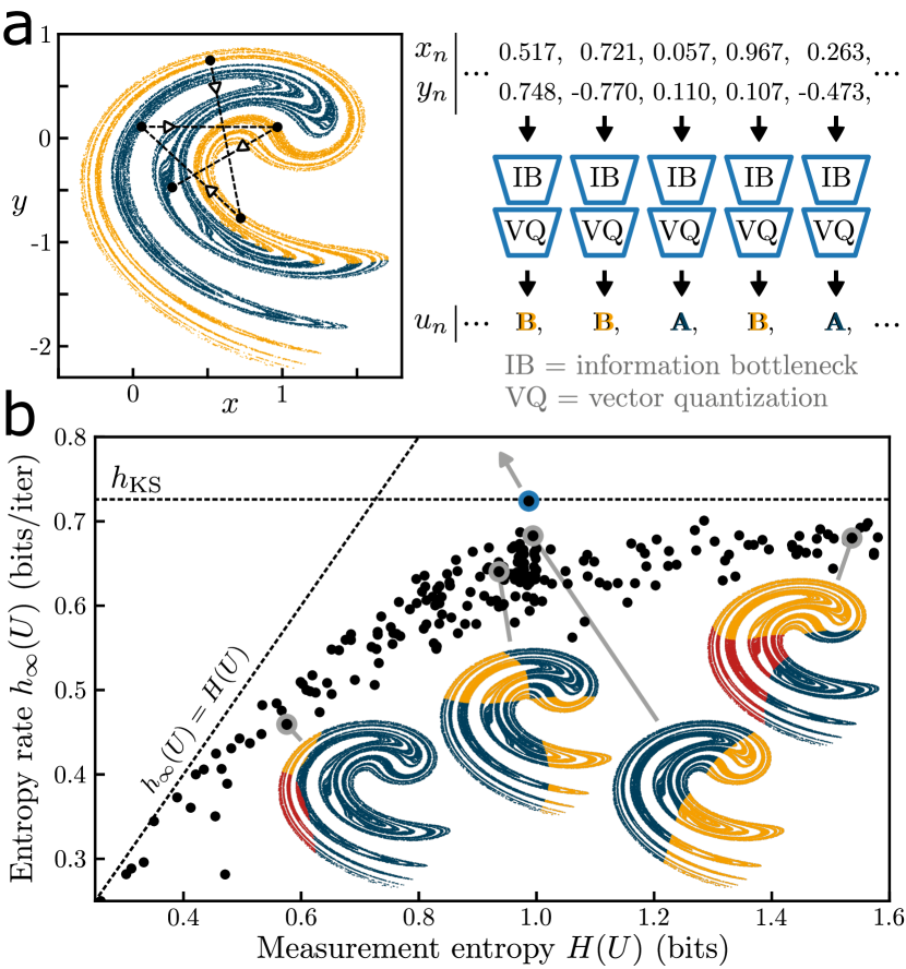
Figure 1: Measurement schemes for the Ikeda map. (a) The attractor of the Ikeda map and several points of a trajectory. An optimal measurement of the continuous-valued state to a discrete-valued outcome is called a generating partition. States colored blue (orange) are measured as outcome A (B). The proposed method optimizes the measurement of a chaotic system using artificial neural networks that apply the information bottleneck and vector quantization to each continuous-valued state. For an optimal measurement and in the asymptotic limit, the sequence of discrete measurements contains the same information as the sequence of continuous-valued states from which it was derived. (b) The space of possible discrete measurements visualized in terms of the entropy of a single measurement, $H(U)$, and the rate of entropy production in the infinite duration limit, $h_{\infty}(U)$. The largest attainable entropy rate is the metric entropy $h_{\textnormal{KS}}$, and is achievable with a generating partition. The blue point corresponds to the approximate generating partition in panel a as identified by the proposed method. The black points correspond to discrete measurements parameterized by neural networks with randomly sampled weights (details in Supp.).

Let a state $x\in\mathcal{M}$ exist in $\mathbb{R}^{d}$, where $d$ is the dimension of the state space. A map $\mathcal{F}(x):\mathcal{M}\rightarrow\mathcal{M}$ propagates a state forward in time by one iteration, i.e. $\mathcal{F}(x_{n})=x_{n+1}$. We consider only discrete time maps in this work, though the analysis is as applicable to straightforward discretizations of continuous-time flows [eckmannruelle1985]. The dynamics are fully described by the map above, but a probabilistic view is often more natural [nicolis2012foundations] and allows us to utilize information theory. For ergodic dynamical systems, which will be our concern in this work, the natural probability distribution over states $p(x)$ is an invariant measure, $\mathcal{F}(p(x))=p(x)$, and can be obtained by iterating forward a long trajectory [eckmannruelle1985].

Given a probability distribution over states, we can define a random variable $X_{n}$ for the state at timestep $n$, and a random process $\bm{X}_{n:n+L}$ for a sequence of random variables $X_{n},X_{n+1},...,X_{n+L-1}$. For a stationary process, the start of the trajectory is unimportant, and instead we consider the statistics of subsequences of length $L$, which we denote $\bm{X}_{L}$.

A continuous-valued state can be measured, and specifically, discretized, through the use of a partition that divides the support of $p(x)$ into disjoint subsets $\mathcal{A}_{i}$ [kennelbuhl2003gp]. The outcome of a measurement, a random variable $U=f(X)$, converts the continuous-valued state to the index of the subset to which it belongs. Thus a sequence $\bm{X}_{L}$ is replaced by a sequence of discrete measurements $\bm{U}_{L}$.

How much information does a measurement $U$ convey about the original state $X$? Intuitively, information gained serves to reduce uncertainty. The amount of uncertainty about the outcome of a random variable $Z$ may be quantified via the Shannon entropy, $H(Z)=\mathbb{E}_{z\sim p(z)}[-\textnormal{log}\ p(z)]$ [shannon1948mathematical]. The mutual information contained in two random variables is given by the reduction of entropy in one variable after finding the value of the other, $I(Z_{1};Z_{2})=H(Z_{1})-H(Z_{1}|Z_{2})$ [cover1999elements]. The act of measuring a state—by recording in which subset of a partition it resides—conveys $I(U;X)=H(U)$ bits of information because the mapping from $X$ to $U$ is deterministic (i.e., $H(U|X)=0$).

As a random process plays out, entropy is generated from the uncertainty about each subsequent outcome. For a repeated discrete measurement $\bm{U}_{L}$ the amount of generated entropy is equivalent to the accumulated information about the underlying trajectory $\bm{X}_{L}$. The entropy rate is defined as the average entropy generated per step in the limit where the sequence length becomes infinite, $h_{\infty}(U)=\lim_{L\rightarrow\infty}H(\bm{U}_{L})/L$ [cover1999elements]. The largest achievable entropy rate of any partition $U$ is the KS entropy [eckmannruelle1985],

$$h_{\textnormal{KS}}=\sup_{U}h_{\infty}(U).$$ (1)

A partition $U$ whose entropy rate is equal to $h_{\textnormal{KS}}$ is a generating partition [cohenprocaccia1985]. While a “trivial” generating partition can be approximated by a fine discretization of state space [cohenprocaccia1985], there often exist generating partitions which are coarse, with minimal entropy [kennelbuhl2003gp]. Fig. 1a shows an approximate generating partition of the Ikeda map, whose corresponding infinite sequence of observations $...BBABA...$ contains the same information as the continuous-valued trajectory.

A coarse generating partition is desirable because it leverages the specific transformation $\mathcal{F}$ in order to convey minimal redundant information that would be gathered at multiple points in the trajectory. A maximally coarse generating partition $U^{*}$ can be defined as

$$U^{*}=\operatorname*{arg\,min}_{U:h_{\infty}(U)=h_{\text{KS}}}H(U).$$ (2)

Given the restriction to discrete measurements, we can rewrite Eqn. 2 in terms of mutual information rather than entropy, to more closely resemble a rate-distortion function [cover1999elements],

$$U^{*}=\operatorname*{arg\,min}_{U:\lim_{L\rightarrow\infty}I(\bm{U}_{L};\bm{X}_{L})/L=h_{\text{KS}}}I(U;X).$$ (3)

The constrained optimization of Eqn. 3 is more manageable as a Lagrangian cost function $\mathcal{L}$, with $U^{*}=\operatorname*{arg\,min}\mathcal{L}$. We relax the constraint of a specific entropy rate to instead define with the Lagrangian a Pareto front of optimal partitions, and the optimum with maximal entropy rate corresponds to the coarsest generating partition $U^{*}$. By replacing the entropy rate’s infinite limit with a large but finite $L$, we recover the Lagrangian for the distributed IB [aguerri2018DIB, dib_ml],

$$\mathcal{L}=-I(\bm{U}_{L};\bm{X}_{L})+\beta\sum_{i}^{L}I(U_{i};X_{i}),$$ (4)

where $\beta$ is the parameter that determines the relative weighting of the two terms in the Lagrangian. Note: we have made use of the fact that $X$ is stationary, so that $I(U;X)=\sum^{L}_{i}I(U_{i};X_{i})/L$. In contrast to previous applications of the distributed IB [aguerriDVIB2021, steiner2021distributedcompression, dib_ml], the trajectory $\bm{X}_{L}$ serves both as the input composite random variable and as the relevance random variable.

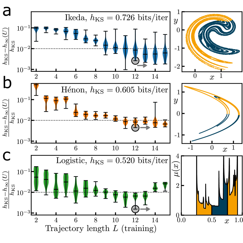
Figure 2: Entropy rate of optimized partitions and the trajectory length during training. The fractional deviation of the entropy rate $h_{\infty}(U)$ from the metric entropy $h_{\text{KS}}$ as a function of the length of the trajectory $L$ used for training for (a) Ikeda and (b) Hénon maps with standard parameters, and (c) the logistic map with $r=3.7115$. The distribution of values of the entropy rate over 20 trials for each $L$ are shown as violin plots, with the extrema and median indicated by the black horizontal marks; the dotted line indicates $h_{\infty}(U)=0.99h_{\text{KS}}$. For each system, the partition found with the largest entropy rate for $L=12$ is shown on the right. For the logistic map, the probability density of states $p(x)$ is colored according to the optimized partition.

The space of possible partitions is vast, filled with colorings of the attractor that encapsulate suboptimal information [bollt2001misplaced, cafaro2015causation]. Fig. 1b displays example partitions of the Ikeda map by their single measurement entropy $H(U)$ and by their entropy rate, $h_{\infty}(U)$, which is upper bounded by $H(U)$ and $h_{\textnormal{KS}}$. By replacing the mutual information terms in Eqn. 4 with appropriate bounds—namely InfoNCE [oord2018InfoNCE] as a lower bound on $I(\bm{U}_{L};\bm{X}_{L})$ and the variational upper bound central to variational autoencoders on $I(U_{i};X_{i})$ [betavae, alemiVIB2016]—we can optimize the distributed IB with machine learning and leverage the expressivity of deep learning to search the space of partitions [alemiVIB2016, aguerriDVIB2021, dib_ml].

To map a state $x$ to a measurement $u$, we followed a two-step process, where each step was performed by a distinct multilayer perceptron (MLP) (Fig. 1a). First $x$ was mapped to an intermediate latent space where the information penalty was enforced by a variational information bottleneck [alemiVIB2016], and then the outcome was passed through a vector quantization MLP. To perform the vector quantization, we followed a method that parameterizes the spectrum of soft-to-hard compression schemes (a soft compression has $H(U|X){>}0$) and gradually hardens over the course of training [agustsson2017softtohard]. Successful partitions were obtained without requiring a hardening schedule; instead a simple discontinuous hardening was applied after training. For a sequence of length $L$, all states $\bm{x}_{:L}$ were ‘measured’ and then the corresponding measurements $\bm{u}_{:L}$ were processed together by another MLP to predict a reference state from the original sequence, e.g. $x_{1}$. For a chaotic system, a single continuous-valued state contains the same information as the infinite trajectory; we found optimization to fail when matching with the full sequence of length $L$. The magnitude of the information penalty $\beta$ was annealed to gradually allow more information into the measurement process, $I(U;X)$. Training began with no information passing through to the measurement $U$ and then stopped after $I(U;X)$ exceeded one bit. Architecture and training details are in the Supp.

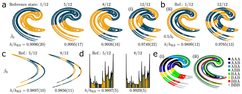
Figure 3: Influence of training parameters on the optimized partitions. (a) For the Ikeda map, the reference state (i.e., the one predicted from the sequence of measurements) strongly influences the optimized partition. Each partition displayed had the largest entropy rate out of ten trials. Coordinate axes have been suppressed. (b) The same as in panel a, but with half the rate of information annealing $\dot{\beta}$ during training. (c) Two of the partitions of the Hénon map, identified with the same annealing rate as in panel a. (d) Same as in panel c for the logistic map with $r=3.7115$. (e) Colorings of the Ikeda attractor where, given a sequence of three measurements $\bm{u}_{:3}$, the final state $x_{3}$ is predicted, utilizing for the measurement $U$ the partition labelled (i) (left) and (ii) (right) in a and b, respectively. Partition (i) yields a simpler coloring than partition (ii) when predicting the final state of a sequence of three iterations.

To quantify the performance of an optimized measurement, we used the difference between the known metric entropy and the measurement’s entropy rate, quantifying the amount of information per step that the measurement fails to capture. Estimating the entropy rate from finite sequences of symbols is challenging, with several methods proposed over the years [schurmanngrassberger1996, kennel2002ctw, nemenman2004entropy, gao2008estimating, martiniani2019quantifying]. We used a form of data compression known as context tree weighting [willems1995ctw], and estimated $h_{\infty}(U)$ from finite size scaling with the ansatz proposed in schurmanngrassberger1996. While strict equivalence between the distributed IB and a maximally coarse generating partition is valid only in the limit $L\rightarrow\infty$, we found that $L\approx 10$ was sufficient to consistently find partitions with an entropy rate at least $0.99h_{\text{KS}}$ for the chaotic maps studied (Fig. 2). Partitions with the largest $h_{\infty}(U)$ found for $L=12$ are shown on the right.

The generating partition for a map is not unique [jaegerkantz1997]. Any of the infinite forward or reverse iterates of a generating partition is also one; additionally there can be nontrivial variants that cross through certain homoclinic tangencies, where the stable and unstable manifolds run parallel to one another [jaegerkantz1997]. We found that certain details of the training process steered optimization to qualitatively different partitions (Fig. 3). Varying the reference state drove the optimization to different iterates of the same base partition (Fig. 3a-d; iterates in Supp.), and a slower annealing of the information $\dot{\beta}$ reached deeper into the forward and backward iterates of the base partition (Fig. 3b). The different iterates require simpler or more complicated functions to integrate multiple measurements (Fig. 3e); the iterates found through optimization allow for simpler integration functions. The base partition found for the Ikeda map (Fig. 3a, reference state 5/12) closely resembles what has been found in prior work [davidchack2000UPOs, kennelbuhl2003gp, hirata2004shadowing, ghalyan2018locally]. For the Hénon and logistic maps, the base partitions (shown in Fig 2) are slight variations of reported generating partitions [grassberger1985henon, schurmanngrassberger1996].

In this Letter, we established an equivalence between the definition of a maximally coarse generating partition and the distributed information bottleneck, and leveraged the equivalence to optimize measurement of a chaotic dynamical system with machine learning. Operating without knowledge of the dynamics and without reliance on properties specific to generating partitions such as the unique description of periodic orbits [davidchack2000UPOs], homoclinic tangencies [grassberger1985henon, jaegerkantz1997, mitchell2012partitioning, chai2021symbolic], or the Koopman operator [zhang2022koopman], the method is not restricted to chaotic systems. Instead, the deterministic chaos serves as a testbed where the notion of an optimal measurement scheme has been made precise and can be quantitatively evaluated. Optimizing a measurement to extract maximal information about an underlying state is a broad goal in understanding inference in biological and computational systems. Prior research has predominantly focused on a singular compression that extracts maximal information from the present and/or past about the future [creutzig2009PIB, still2010optimal, palmer2015predictive, marzen2016predictive]. A notable exception is the recursive information bottleneck [still2014information], in which a sequence of measurements are recursively aggregated and each step’s measurement scheme can vary based on what has been previously observed. By contrast, the distributed information bottleneck setup of this work optimizes a fixed measurement scheme that is repeatedly applied for maximal aggregate information, a plausible scenario for sensing organisms or sensory devices.

The current study focused exclusively on relatively simple chaotic maps that have been well characterized so as to establish the capabilities of the proposed method. The variegated faces of chaos present exciting opportunities for the optimization of measurement processes and can serve as a rich testbed for machine learning methods of compression [oord2017vqvae, jang2016categorical, gilpin2023forecast]. In the large majority of systems where there is no precedent generating partition with which to compare, the metric entropy can be readily estimated from data [cohenprocaccia1985, wales1991calculating] and other means of quantitatively evaluating partitions can be used [plumecoq2000templateanalysisII] to ground the measurement schemes learned by the proposed method.

To our knowledge, the connection between metric entropy and a rate-distortion objective was previously unconsidered in the literature. The transformation $\mathcal{F}$ whose repeated application creates the strange attractor evolves points in state space such that a fixed measurement continually acquires new information about the continuous-valued trajectory ad infinitum. The maximally coarse generating partition is the minimally redundant lossy compression of the attractor that can uniquely identify every trajectory given an infinite time horizon. By optimizing the lossy compression, the spawned information that serves to limit predictability for any finite model is manifest as a specific coloring of the attractor that divides state space with a remarkably crude, yet highly specific cut.

I Acknowledgements

We gratefully acknowledge Sam Dillavou, Sarah Marzen and Kevin A. Mitchell for helpful discussions, and Jason Z. Kim, and Suman Kulkarni for comments on the manuscript.

 

Supplemental Material

S1 Code availability

The full code base has been released on Github at the following location: distributed-information-bottleneck.github.io. Every analysis included in this work can be repeated from scratch in Google Colab with the iPython notebook in this directory.

S2 Appendix A: The chaotic maps studied

We studied three chaotic maps in this work. The logistic map [beck1995thermodynamics],

$$x_{n+1}=rx_{n}(1-x_{n}),$$ (5)

is a one-dimensional map defined over the unit interval. We used the value $r=3.7115$ for the main text, and additionally used $r=4$ to benchmark the entropy rate estimation in App. B. The Hénon map [grassberger1985henon],

$$\begin{split}x_{n+1}&=1-ax_{n}^{2}+by_{n}\\ y_{n+1}&=x_{n},\end{split}$$ (6)

is a two-dimensional map, and we used the extensively studied parameters $a=1.4$, $b=0.3$. Finally, the Ikeda map [ikeda1979],

$$\begin{split}\phi&=\kappa-\eta/(1+x_{n}^{2}+y_{n}^{2})\\ x_{n+1}&=a+b(x_{n}\cos(\phi)-y_{n}\sin(\phi))\\ y_{n+1}&=b(x_{n}\sin(\phi)-y_{n}\cos(\phi)),\end{split}$$ (7)

is another two-dimensional map, and we again followed precedent with the parameters $a=1$, $b=0.9$, $\kappa=0.4$, $\eta=6$ [davidchack2000UPOs].

S3 Appendix B: Estimation of entropy rate

Given a sequence of symbols that can take any of a discrete set of values, we wish to estimate the asymptotic rate of entropy produced per symbol,

$$h_{\infty}(U)=\lim_{L\rightarrow\infty}\frac{H(\bm{U}_{L})}{L}=\lim_{L\rightarrow\infty}H(U_{L}|\bm{U}_{L-1}).$$ (8)

The second equality holds in the case of stationary processes [gao2008estimating] and makes clearer the interpretation of the entropy rate as the rate of information creation.

The entropy rate can be at most $H(U)$, when every symbol is independent from the rest, as is the case for a sequence of coin flips. Regularity in the process reduces the entropy rate, and the lowest entropy rate of zero corresponds to determinism in the symbolic dynamics (e.g., a periodic signal). Note the distinction between determinism in the symbolic dynamics, where every symbol is known with certainty given the past, and determinism in the continuous-valued state space. The latter can yield uncertainty given only the results of discrete measurements, which have discarded information.

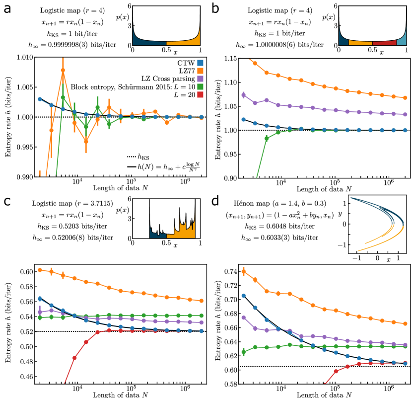
Supplemental Material, Figure S1: Estimating entropy rate. (a) The logistic map ($r=4$) generating partition with two symbols; $h_{\textnormal{KS}}=1$ bit per iteration of the map. (b) The logistic map ($r=4$) generating partition with four symbols; $h_{\textnormal{KS}}=1$ bit per iteration of the map. (c) The logistic map ($r=3.7115$) generating partition with two symbols; $h_{\textnormal{KS}}=0.5203$ bit per iteration of the map. (d) The Hénon map ($a=1.4,b=0.3$); $h_{\textnormal{KS}}=0.6048$ bits per iteration of the map. Error bars indicate the standard error from five repeats.

Methods of file compression leverage regularities in the bit stream of a file, and commonly form the basis for estimates of entropy rate. Lempel-Ziv (LZ) compression, of which there are several variants, constructs a codebook of previously unobserved sequences during a single pass through the data. Context tree weighting (CTW) is another method of file compression that constructs a suffix tree storing every subsequence contained in the data. While LZ compression is fast to compute, the meticulous record keeping of CTW converges more quickly with file size to the entropy rate [kennel2002ctw]. We implemented the infinite depth CTW following kennel2005bayesian; the C++ code may be found in the linked repository.

We compare in Fig. S1 various estimates of the entropy rate for generating partitions of the logistic and Hénon maps where $h_{\textnormal{KS}}$ and generating partitions are known. We included a cross parsing variant of LZ whereby a codebook is made with one sequence of length $L$ and evaluated on another [ro2022xparse]. Additionally, we compared to a bias-corrected form of block entropy [schurmann2015blockent], based on the entropy of subsequences of length $B$. Even with the bias correction, estimating the entropy rate using block entropy is problematic because there is often no indication about what length $B$ yields the best estimate [kennel2005bayesian]. Here and for all other entropy rate estimates in the manuscript, sequences of fifteen lengths $L$ logarithmically spaced between two thousand and two million were randomly selected from a dataset of 20 million points. Five repeats were evaluated for each $L$.

We found that the convergence of CTW, while faster than LZ, was highly variable for different partitions, and that computing the entropy rate from CTW for a reasonably large file size would not suffice in general. Instead, we followed schurmanngrassberger1996, who fit an ansatz of sequence length dependence of the entropy rate measured via construction of a suffix tree (though not CTW). We found the same ansatz to work well for the finite size scaling of the CTW estimates,

$$h_{N}=h_{\infty}+c\frac{\log N}{N^{\gamma}},$$ (9)

and used nonlinear least squares (scipy.optimize.curve_fit) for the estimate of $h_{\infty}$ and its standard error.

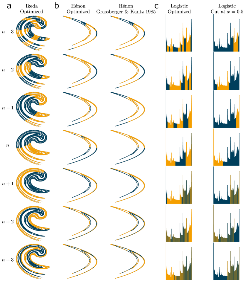
Supplemental Material, Figure S2: Iterates of optimized partitions and established generating partitions. The partitions in the gray box, labelled timestep $n$, were iterated forward and backward three steps while retaining the coloring from timestep $n$. Coordinate axes have been suppressed. (a) The Ikeda map, with the partition at timestep $n$ the result of a run with $L=12$ and reference timestep $6/12$. (b) The Hénon map with standard parameters, optimized with the current method on the left and found by grassberger1985henon by threading certain homoclinic tangencies. (c) The logistic map with $r=3.7115$, optimized with the current method on the left and the known GP, with a boundary at the critical point at $x=0.5$ (true for any value of $r$). The invariant measure $p(x)$ is displayed vertically, and the bins are shaded according to the proportion of partition assignments at timestep $n$.

S4 Appendix C: Machine learning implementation details

All experiments were implemented in TensorFlow and run on a single computer with a 12 GB GeForce RTX 3060 GPU. Each optimization and its entropy rate estimation took several minutes.

For all maps, subsequences of length $L$ iterations were randomly sampled from a sequence of length $10^{6}$ for training, and every $x_{i}$ was individually compressed by the same two-step encoder. The first stage of the encoder was a multilayer perceptron (MLP) with two layers of 128 units each and LeakyReLU activations, followed by a final projection to 8-dimensional “information bottleneck” space over $\tilde{U}$. The second stage was another MLP with two layers of 128 LeakyReLU units, taking $\tilde{U}$ to the soft discretization space over $U$: a two dimensional space followed by a softmax activation.

In the information bottleneck space, transmitted information was penalized through the Kullback-Leibler (KL) divergence between the encoded conditional distributions $p(\tilde{u}|x)$ and the prior $r(\tilde{u})$, a standard normal distribution $\mathcal{N}(\bm{0},\bm{1})$. As is typical for variational autoencoders [vae], the conditional distributions were parameterized as Gaussians with diagonal covariance matrices. Values were sampled from the conditional distributions following the reparameterization trick [vae], and the sampled values $\tilde{u}$ were passed through the second stage. The softmax activation mapped embeddings to a probability distribution over two outcomes (representing assignment to a binary partition). The temperature parameter in the softmax was taken to be one during training and changed to zero discontinuously after training (i.e., making the partition assignment an arg max operation on the probability vector).

The $L$ embeddings $u_{1},...,u_{L}$ were then concatenated and passed as input to the predictive model, $g(u_{1},...,u_{L})$, an MLP consisting of two layers of 256 units with LeakyReLU activation, followed by a linear projection to 32 dimensions (i.e., a final dense layer with 32 units and no activation function). The 32-dimensional space was shared with the output of a reference state encoder $h(x_{\text{ref}})$, another MLP with two layers of 256 units with LeakyReLU activation, followed by a linear projection to 32 dimensions. In this 32-dimensional shared latent space the InfoNCE loss [oord2018InfoNCE] was evaluated by pairing up each length $L$ trajectory with its reference state, using the squared Euclidean distance as a measure of similarity between the embedding vectors. The remainder of the batch size of 2048 provided negative samples for the InfoNCE loss.

To traverse the low information Pareto front, we used nonlinear IB [kolchinsky2019nonlinear], squaring the information bottleneck penalty ($I(U_{i};X_{i})$) in the Lagrangian (Eqn. 4 in the main text). The loss was

$$\mathcal{L}_{\textnormal{VIB}}=\mathcal{L}_{\text{InfoNCE}}(g(u_{1},...,u_{L}),h(x_{\text{ref}}))+\beta\sum_{i}^{L}\left(D_{\textnormal{KL}}(p(\tilde{u}_{i}|x_{i})||r(\tilde{u}))\right)^{2}.$$ (10)

We decreased $\beta$ in equally spaced logarithmic steps from $10$ to $10^{-4}$ over 20,000 steps, and stopped once the information per measurement $I(U;X)$ exceeded one bit (with $I(U;X)$ estimated as in Ref. [dib2] using lower and upper bounds from poole2019variational). The Adam optimizer was used with a learning rate of $3\times 10^{-4}$.

The low-dimensional continuous-valued states underwent positional encoding, a term from natural language processing that has been used in certain computer vision contexts to facilitate learning on low-dimensional features. Before being passed to the MLP, inputs were mapped to $x\leftarrow(x,\sin\omega_{1}x,\sin\omega_{2}x,...)$) with frequencies $\omega_{k}=2^{k}$ where $k\in\{1,2,...10\}$ [dib_ml].

After training concluded, there remained a difficulty around how to use the conditional distributions in the bottleneck space. The embeddings are the distributions; we sampled from them during training thanks to the reparameterization trick, but sampling during the conversion to a partition would leave stochasticity in the assignment, i.e. $H(U|X){>}0$. We can instead view the distribution in the information bottleneck space as an ensemble of hard partitions, and the transmitted information is the degree to which the downstream layers can “pinpoint” the member of the ensemble. From this perspective it becomes sensible to sample a fixed number of noise vectors, representing as many members of the ensemble, and use those noise vectors to assign each $x$ to a $u$. The majority assignment of each point is then used for the partition, sans stochasticity.

S4.1 Randomly sampled discrete measurements (Fig. 1 of main text)

To generate a random sample of discrete measurements, we initialized MLPs with 1, 2, and 3 layers of 64 units each, with ReLU or tanh activation. The weights and biases were sampled from a normal distribution with a mean of 0.05 and a standard deviation of 0.5. The dimension of the input was 2, corresponding to the coordinates of the Ikeda map, and the output dimension was 2 or 4, corresponding to the alphabet size for the measurement (i.e., the number of colors). The continuous-valued outputs, one for each input point, were discretized by selecting the dimension in the output with the largest absolute value. 20 networks were sampled for each configuration (number of layers, activation, alphabet size), for 240 in total.

S5 Appendix D: Iterates of partitions found in the paper

We display in Fig. S2 three forward and three reverse iterations of partitions for the Ikeda, Hénon , and logistic maps studied in this work. The optimized partitions for the Hénon and logistic maps differ from previously reported generating partitions, with modifications that increase the entropy: 0.94 bits up from 0.91 bits for Hénon, and 0.99 bits up from 0.82 bits for the logistic map.

S6 Appendix E: Citation Diversity Statement

Science is a human endeavour and consequently vulnerable to many forms of bias; the responsible scientist identifies and mitigates such bias wherever possible. Meta-analyses of research in multiple fields have measured significant bias in how research works are cited, to the detriment of scholars in minority groups [maliniak2013gender, caplar2017quantitative, chakravartty2018communicationsowhite, dion2018gendered, dworkin2020extent, teich2022citation]. We use this space to amplify studies, perspectives, and tools that we found influential during the execution of this research [zurn2020citation, dworkin2020citing, zhou2020gender, budrikis2020growing]. We sought to proactively consider choosing references that reflect the diversity of the field in thought, form of contribution, gender, race, ethnicity, and other factors. The gender balance of papers cited within this work was quantified using a combination of automated gender-api.com estimation and manual gender determination from authors’ publicly available pronouns. By this measure (and excluding self-citations to the first and last authors of our current paper), the references of the main text contain 3% woman(first)/woman(last), 7% man/woman, 16% woman/man, and 74% man/man. This method is limited in that a) names, pronouns, and social media profiles used to construct the databases may not, in every case, be indicative of gender identity and b) it cannot account for intersex, non-binary, or transgender people. We look forward to future work that could help us to better understand how to support equitable practices in science.

References

- Shaw [1981] R. Shaw, Zeitschrift für Naturforschung A 36, 80 (1981).
- Eckmann and Ruelle [1985] J.-P. Eckmann and D. Ruelle, Reviews of modern physics 57, 617 (1985).
- Tsonis and Elsner [1989] A. Tsonis and J. Elsner, Bulletin of the American Meteorological Society 70, 14 (1989).
- Slingo and Palmer [2011] J. Slingo and T. Palmer, Philosophical Transactions of the Royal Society A: Mathematical, Physical and Engineering Sciences 369, 4751 (2011).
- Kargarnovin et al. [2023] S. Kargarnovin, C. Hernandez, F. V. Farahani, and W. Karwowski, Brain Sciences 13, 813 (2023).
- Skinner et al. [1992] J. E. Skinner, M. Molnar, T. Vybiral, and M. Mitra, Integrative Physiological and Behavioral Science 27, 39 (1992).
- Nicolis and Nicolis [2012] G. Nicolis and C. Nicolis, Foundations of complex systems: emergence, information and predicition (World Scientific, 2012).
- Bradley and Kantz [2015] E. Bradley and H. Kantz, Chaos: An Interdisciplinary Journal of Nonlinear Science 25 (2015).
- Wales [1991] D. J. Wales, Nature 350, 485 (1991).
- Pathak et al. [2018] J. Pathak, B. Hunt, M. Girvan, Z. Lu, and E. Ott, Physical review letters 120, 024102 (2018).
- Amil et al. [2019] P. Amil, M. C. Soriano, and C. Masoller, Chaos: An Interdisciplinary Journal of Nonlinear Science 29 (2019).
- Tang et al. [2020] Y. Tang, J. Kurths, W. Lin, E. Ott, and L. Kocarev, Chaos: An Interdisciplinary Journal of Nonlinear Science 30, 063151 (2020).
- Gilpin [2023] W. Gilpin, arXiv preprint arXiv:2303.08011 (2023).
- Williams [2004] S. G. Williams, in Proceedings of symposia in applied mathematics, Vol. 60 (2004) pp. 1–12.
- Béal and Perrin [2013] M.-P. Béal and D. Perrin, in Handbook of Formal Languages: Volume 2. Linear Modeling: Background and Application (Springer, 2013) pp. 463–506.
- Lind and Marcus [2021] D. Lind and B. Marcus, An introduction to symbolic dynamics and coding (Cambridge university press, 2021).
- Hirata and Amigó [2023] Y. Hirata and J. M. Amigó, Chaos: An Interdisciplinary Journal of Nonlinear Science 33 (2023).
- Ray [2004] A. Ray, Signal processing 84, 1115 (2004).
- Hayes et al. [1994] S. Hayes, C. Grebogi, E. Ott, and A. Mark, Physical Review Letters 73, 1781 (1994).
- James et al. [2014] R. G. James, K. Burke, and J. P. Crutchfield, Physics Letters A 378, 2124 (2014).
- Gaspard and Wang [1993] P. Gaspard and X.-J. Wang, Physics Reports 235, 291 (1993).
- Beck and Schögl [1993] C. Beck and F. Schögl, Thermodynamics of chaotic systems, Cambridge nonlinear science series (Cambridge University Press, 1993).
- Schürmann and Grassberger [1996] T. Schürmann and P. Grassberger, Chaos: An Interdisciplinary Journal of Nonlinear Science 6, 414 (1996).
- Cohen and Procaccia [1985] A. Cohen and I. Procaccia, Physical review A 31, 1872 (1985).
- Badii and Politi [1997] R. Badii and A. Politi, Complexity: Hierarchical Structures and Scaling in Physics, Cambridge nonlinear science series (Cambridge University Press, 1997).
- Kennel and Buhl [2003] M. B. Kennel and M. Buhl, Physical Review Letters 91, 084102 (2003).
- Ikeda [1979] K. Ikeda, Optics communications 30, 257 (1979).
- Grassberger and Kantz [1985] P. Grassberger and H. Kantz, Physics Letters A 113, 235 (1985).
- Davidchack et al. [2000] R. L. Davidchack, Y.-C. Lai, E. M. Bollt, and M. Dhamala, Physical Review E 61, 1353 (2000).
- Plumecoq and Lefranc [2000] J. Plumecoq and M. Lefranc, Physica D: Nonlinear Phenomena 144, 259 (2000).
- Mitchell [2012] K. A. Mitchell, Physica D: Nonlinear Phenomena 241, 1718 (2012).
- Chai and Lan [2021] M. Chai and Y. Lan, Chaos: An Interdisciplinary Journal of Nonlinear Science 31 (2021).
- Zhang et al. [2022] C. Zhang, H. Li, and Y. Lan, Chaos: An Interdisciplinary Journal of Nonlinear Science 32 (2022).
- Estella Aguerri and Zaidi [2018] I. Estella Aguerri and A. Zaidi, in International Zurich Seminar on Information and Communication (IZS 2018). Proceedings (ETH Zurich, 2018) pp. 35–39.
- Murphy and Bassett [2023a] K. A. Murphy and D. S. Bassett, in The Eleventh International Conference on Learning Representations (2023).
- Tishby et al. [2000] N. Tishby, F. C. Pereira, and W. Bialek, arXiv preprint physics/0004057 (2000).
- Murphy and Bassett [2023b] K. A. Murphy and D. S. Bassett, arXiv preprint arXiv:2307.04755 (2023b).
- Shannon [1948] C. E. Shannon, The Bell System Technical Journal 27, 379 (1948).
- Cover and Thomas [1999] T. M. Cover and J. A. Thomas, Elements of information theory (John Wiley & Sons, 1999).
- Aguerri and Zaidi [2021] I. E. Aguerri and A. Zaidi, IEEE Transactions on Pattern Analysis and Machine Intelligence 43, 120 (2021).
- Steiner and Kuehn [2021] S. Steiner and V. Kuehn, in ICC 2021 - IEEE International Conference on Communications (2021) pp. 1–6.
- Bollt et al. [2001] E. M. Bollt, T. Stanford, Y.-C. Lai, and K. Życzkowski, Physica D: Nonlinear Phenomena 154, 259 (2001).
- Cafaro et al. [2015] C. Cafaro, W. M. Lord, J. Sun, and E. M. Bollt, Chaos: An interdisciplinary journal of nonlinear science 25 (2015).
- Oord et al. [2018] A. v. d. Oord, Y. Li, and O. Vinyals, arXiv preprint arXiv:1807.03748 (2018).
- Higgins et al. [2017] I. Higgins, L. Matthey, A. Pal, C. Burgess, X. Glorot, M. Botvinick, S. Mohamed, and A. Lerchner, in International Conference on Learning Representations (2017).
- Alemi et al. [2017] A. A. Alemi, I. Fischer, J. V. Dillon, and K. Murphy, in International Conference on Learning Representations (2017).
- Agustsson et al. [2017] E. Agustsson, F. Mentzer, M. Tschannen, L. Cavigelli, R. Timofte, L. Benini, and L. V. Gool, in Advances in Neural Information Processing Systems, Vol. 30 (2017).
- Kennel and Mees [2002] M. B. Kennel and A. I. Mees, Physical Review E 66, 056209 (2002).
- Nemenman et al. [2004] I. Nemenman, W. Bialek, and R. de Ruyter van Steveninck, Phys. Rev. E 69, 056111 (2004).
- Gao et al. [2008] Y. Gao, I. Kontoyiannis, and E. Bienenstock, Entropy 10, 71 (2008).
- Martiniani et al. [2019] S. Martiniani, P. M. Chaikin, and D. Levine, Physical Review X 9, 011031 (2019).
- Willems et al. [1995] F. M. Willems, Y. M. Shtarkov, and T. J. Tjalkens, IEEE transactions on information theory 41, 653 (1995).
- Jaeger and Kantz [1997] L. Jaeger and H. Kantz, Journal of Physics A: Mathematical and General 30, L567 (1997).
- Hirata et al. [2004] Y. Hirata, K. Judd, and D. Kilminster, Physical Review E 70, 016215 (2004).
- Ghalyan et al. [2018] N. F. Ghalyan, D. J. Miller, and A. Ray, Neural computation 30, 2500 (2018).
- Creutzig et al. [2009] F. Creutzig, A. Globerson, and N. Tishby, Physical Review E 79, 041925 (2009).
- Still et al. [2010] S. Still, J. P. Crutchfield, and C. J. Ellison, Chaos: An Interdisciplinary Journal of Nonlinear Science 20 (2010).
- Palmer et al. [2015] S. E. Palmer, O. Marre, M. J. Berry, and W. Bialek, Proceedings of the National Academy of Sciences 112, 6908 (2015).
- Marzen and Crutchfield [2016] S. E. Marzen and J. P. Crutchfield, Journal of Statistical Physics 163, 1312 (2016).
- Still [2014] S. Still, Entropy 16, 968 (2014).
- Van Den Oord et al. [2017] A. Van Den Oord, O. Vinyals, and K. Kavukcuoglu, Advances in neural information processing systems 30 (2017).
- Jang et al. [2017] E. Jang, S. Gu, and B. Poole, in International Conference on Learning Representations (2017).

References

- Beck and Schögl [1993] C. Beck and F. Schögl, Thermodynamics of chaotic systems, Cambridge nonlinear science series (Cambridge University Press, 1993).
- Grassberger and Kantz [1985] P. Grassberger and H. Kantz, Physics Letters A 113, 235 (1985).
- Ikeda [1979] K. Ikeda, Optics communications 30, 257 (1979).
- Davidchack et al. [2000] R. L. Davidchack, Y.-C. Lai, E. M. Bollt, and M. Dhamala, Physical Review E 61, 1353 (2000).
- Gao et al. [2008] Y. Gao, I. Kontoyiannis, and E. Bienenstock, Entropy 10, 71 (2008).
- Kennel and Mees [2002] M. B. Kennel and A. I. Mees, Physical Review E 66, 056209 (2002).
- Kennel et al. [2005] M. B. Kennel, J. Shlens, H. D. I. Abarbanel, and E. J. Chichilnisky, Neural Computation 17, 1531 (2005), https://direct.mit.edu/neco/article-pdf/17/7/1531/816326/0899766053723050.pdf .
- Ro et al. [2022] S. Ro, B. Guo, A. Shih, T. V. Phan, R. H. Austin, D. Levine, P. M. Chaikin, and S. Martiniani, Physical review letters 129, 220601 (2022).
- Schürmann [2015] T. Schürmann, Neural computation 27, 2097 (2015).
- Schürmann and Grassberger [1996] T. Schürmann and P. Grassberger, Chaos: An Interdisciplinary Journal of Nonlinear Science 6, 414 (1996).
- Kingma and Welling [2014] D. P. Kingma and M. Welling, in International Conference on Learning Representations (ICLR) (2014).
- Oord et al. [2018] A. v. d. Oord, Y. Li, and O. Vinyals, arXiv preprint arXiv:1807.03748 (2018).
- Kolchinsky et al. [2019] A. Kolchinsky, B. D. Tracey, and D. H. Wolpert, Entropy 21, 1181 (2019).
- Murphy and Bassett [2023a] K. A. Murphy and D. S. Bassett, arXiv preprint arXiv:2307.04755 (2023a).
- Poole et al. [2019] B. Poole, S. Ozair, A. Van Den Oord, A. Alemi, and G. Tucker, in International Conference on Machine Learning (PMLR, 2019) pp. 5171–5180.
- Murphy and Bassett [2023b] K. A. Murphy and D. S. Bassett, in The Eleventh International Conference on Learning Representations (2023).
- Maliniak et al. [2013] D. Maliniak, R. Powers, and B. F. Walter, International Organization 67, 889 (2013).
- Caplar et al. [2017] N. Caplar, S. Tacchella, and S. Birrer, Nature Astronomy 1, 1 (2017).
- Chakravartty et al. [2018] P. Chakravartty, R. Kuo, V. Grubbs, and C. McIlwain, Journal of Communication 68, 254 (2018).
- Dion et al. [2018] M. L. Dion, J. L. Sumner, and S. M. Mitchell, Political Analysis 26, 312 (2018).
- Dworkin et al. [2020a] J. D. Dworkin, K. A. Linn, E. G. Teich, P. Zurn, R. T. Shinohara, and D. S. Bassett, Nature Neuroscience 23, 918 (2020a).
- Teich et al. [2022] E. G. Teich, J. Z. Kim, C. W. Lynn, S. C. Simon, A. A. Klishin, K. P. Szymula, P. Srivastava, L. C. Bassett, P. Zurn, J. D. Dworkin, et al., Nature Physics 18, 1161 (2022).
- Zurn et al. [2020] P. Zurn, D. S. Bassett, and N. C. Rust, Trends in Cognitive Sciences 24, 669 (2020).
- Dworkin et al. [2020b] J. Dworkin, P. Zurn, and D. S. Bassett, Neuron 106, 890 (2020b).
- Zhou et al. [2020] D. Zhou, E. J. Cornblath, J. Stiso, E. G. Teich, J. D. Dworkin, A. S. Blevins, and D. S. Bassett, Zenodo (2020).
- Budrikis [2020] Z. Budrikis, Nature Reviews Physics 2, 346 (2020).