d-Wave Hall effect and linear magnetoconductivity in metallic collinear antiferromagnets

Abstract

In this paper we theoretically predict a distinct class of anomalous Hall effects occurring in metallic collinear antiferromagnets. The effect is quadratic and $d-$wave symmetric in external magnetic field. In addition, the electric current, transverse to the current voltage drop and the magnetic field in the predicted effect are all in the same plane. Studied theoretical model consists of two-dimensional fermions interacting with the Neel order through momentum dependent exchange interaction having a $d-$wave symmetry. We also find unusual linear magnetoconductivity in this model.

Anomalous Hall effect is one of the experimental tools which sheds light on the symmetries of the crystal sctructure of the material. The effect primarily requires both time-reversal and inversion symmetry breaking. The details of the crystal structure and magnetic order can drastically vary the anom alous Hall effect. For example, in ferromagnets with magnetization ${\bf M}$ (or Zeeman part of external magnetic field ${\bf B}$) it is expected KarplusLuttinger there will be

$${\bf j}_{\mathrm{AHE}}\propto\left[{\bf M}\times{\bf E}\right],$$ (1)

electric current response, where ${\bf E}$ is the electric field corresponding to the voltage drop. This is the ferromagnetic analog of the regular Hall effect Hall ; Ziman . Main ingredients of anomalous Hall effect in ferromagnets is the combination of the exchange (momentum independent) spin splitting and the spin-orbit coupling Vas'koBychkovRashba ; Dresselhaus ; SovietTI ; Dyakonov of the conducting fermions. For example, two-dimensional fermion system with Rashba spin-orbit coupling and Zeeman-like ferromagnetic exchange is one of the most studied models in relation to the anomalous Hall effect CulcerMacDonaldNiuPRB2003 ; AHE_RMP ; SinitsynPRB2007 ; NunnerPRB2007 . One of the main mechnisms of the anomalous Hall effect is the anomalous part of the fermion velocity KarplusLuttinger which on the other hand is due to the Berry curvature Berry ; BerryReview of conducting fermions.

It is then possible that the anomalous Hall effect can have in-plane configuration Malshukov1998 ; LiuPRL2013 ; ZhangPRB2019 ; Zyuzin2020 ; Culcer2021 ; Kurumaji2023 , where all three vectors, namely the electric current, transverse voltage drop and the magnetization, are in the same, in the example below $x-y$, plane,

$${\bf j}_{\mathrm{IPHE}}\propto\left[\left[{\bf M}\times{\bf e}_{z}\right]\times{\bf e}_{y}\right]\times{\bf E},$$ (2)

here vectors ${\bf e}_{z}$ and ${\bf e}_{y}$ are defined by the spin-orbit coupling. First two vector products filter out only the $M_{y}$ component multiplied by the ${\bf e}_{z}$ unit vector. This effect has been recently experimentally observed in Refs. AHE_ZrTe5 ; Kagome_AHE .

The situation in collinear antiferromagnets is less understood. In simple collinear antiferromagnets, with two sublattices, there is a symmetry under a combination of time-reversal and translation operations which does not allow for spin-splitting of conducting fermions, therefore, making the anomalous Hall effect to vanish. However, microscopic surroundings of each sublattice may make a difference. For example, the aforementioned symmetry will be broken if surroundings of spin up sublattice is different from the surroundings of the spin down. See left plot in Fig. (1) for schematics. The remaining symmetry is a combination of time-reversal and $\frac{\pi}{2}$ rotation operations, which will allow for the spin-splitting of conducting fermions shown in the right plot in Fig. (1).

Research of materials with such a structure started from the seminal work of Pekar and Rashba PekarRashba and have received much of attention since Ogg1966 ; IvchenkoKiselevPTS1992 ; VarmaZhu2006 ; WuSunFradkinZhang2007 ; HayamiYanagiKusunose2019 ; Rashba2020 ; HayamiYanagiKusunose2020 ; EgorovEvarestov ; SmejkalSinovaJungwirth2022a ; SmejkalSinovaJungwirth2022b ; Bose2022 ; Gonzalez-Hernandez2021 ; comment1 . One of the properties of such materials is a giant non-relativistic, due to the antiferromagnetism, spin splitting of conducting fermions HayamiYanagiKusunose2019 ; Rashba2020 ; HayamiYanagiKusunose2020 ; EgorovEvarestov . It is understood that the conducting fermions in, for example, RuO₂, MnF₂, FeSb₂ and many more can be described by such a spin splitting Rashba2020 ; EgorovEvarestov ; SmejkalSinovaJungwirth2022a ; SmejkalSinovaJungwirth2022b . Experimentally measured Bose2022 spin filtered electric transport is one of the manifestations of such spin splitting Gonzalez-Hernandez2021 .

In this paper we show that in addition to known cases of the anomalous Hall effect, given by Eq. (1) and (2), metallic antiferromagnets with spin split conducting fermions described above may show very unusual anomalous Hall effect propoprtional to the second power of the external magnetic field, given by

$${\bf j}_{\mathrm{DWHE}}\propto B_{x}B_{y}\left[{\bf e}_{z}\times{\bf E}\right],$$ (3)

where ${\bf e}_{z}$ is defined by the direction of the Neel vector. We will be referring to it as the d-wave Hall effect. Indeed the $B_{x}B_{y}$ product has the aforementioned symmetry. It is notable that just like in the in-plane Hall effect Eq. (2) all three vectors, namely electric current, transverse voltage drop, and the magnetic field, are in the same plane. Such a response is not prohibited by the Onsager relation, as it is overall cubic in time-reversal symmetry breaking fields, since ${\bf e}_{z}\rightarrow-{\bf e}_{z}$ in Eq. (3) under the time-reversal operation.

In addition to (3) we find another experimentally relevant response,

$${\bf j}_{\mathrm{LMC}}\propto B_{z}\left(E_{x}{\bf e}_{y}+E_{y}{\bf e}_{x}\right),$$ (4)

which, together with regular Hall effect, will result in anisotropic Hall conductivity, i.e. $\sigma_{xy}\neq\sigma_{yx}$. Again, this effect is allowed by Onsager relation because response in (4) is actually quadratic in time-reversal symmetry breaking fields, since $B_{z}$ is selected by Neel order ${\bf e}_{z}$ as $B_{z}\rightarrow({\bf e}_{z}\cdot{\bf B})$ and both change sign under time-reversal.

  

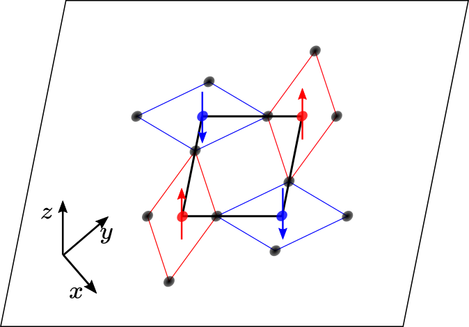
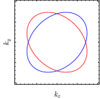
Figure 1: Left: schematics of two-dimensional square lattice in $x-y$ plane with an antiferromagnetic order in $z-$ direction. Red/blue circles correspond to two atoms in the unit cell with spin up/down order. Local environment composed of black circles is different around red/blue atoms. There is a symmetry of $\frac{\pi}{2}$ rotation together with time-reversal: the $\frac{\pi}{2}$ rotation connects local environment of the two elements while the time-reversal flips the spin. Right: Fermi surface of fermions corresponding to Hamiltonian Eq. (5) with $\lambda=0$. Red corresponds to spin up, while blue to spin down.

In order to show the effect, we study a two-dimensional metallic antiferromagnet system shown in left plot in Fig. (1). The Hamiltonian of conducting fermions interacting with the Neel vector and consistent with the lattice symmetry is

$$\hat{H}_{0}=\frac{{\bf k}^{2}}{2m}+\lambda(k_{x}\sigma_{y}-k_{y}\sigma_{x})+\beta\sigma_{z}k_{x}k_{y},$$ (5)

where $\sigma$ are Pauli matrices describing spin of conducting fermions. The term with $\beta$ is the interaction of the conducting fermions with the antiferromagnetic Neel vector. This term breaks the time-reversal symmetry. As noted, it is a combination of difference in atomic configurations around ordered spins and the antiferromagnetic order which generates this term, not just the antiferromagnetic order alone. For example, see left plot in Fig. (1), where a combination of translation and time-reversal symmetries is broken due to the local configuration, while a $\frac{\pi}{2}$ rotation together with the time-reversal is the symmetry of the lattice which supports the term $\beta$. We have included Rashba spin-orbit coupling denoted by $\lambda$. In addition we apply external magnetic field in $x-y$ plane which acts only on spins of fermions (Zeeman magnetic field),

$$\hat{H}_{\mathrm{Z}}=h_{x}\sigma_{x}+h_{y}\sigma_{y},$$ (6)

where ${\bf h}=\frac{1}{2}g\mu_{\mathrm{B}}{\bf B}$, $g$ is the $g-$factor, and $\mu_{\mathrm{B}}$ is the Bohr magneton. Both terms will be needed in our analysis of the electric current responses. We assume that finite electron density with chemical potential $\mu>0$ does not suppress the antiferromagnetic order, as well as the external Zeeman magnetic field does not cant the antiferromagnetically ordered spins in any direction. The latter is plausable if the field is smaller than the magnetic anisotropy which favors $z-$ direction for the Neel vector.

We are interested in electric current responses of this system to external electric field. Let us first understand what kind of responses can be deduced from the symmetry consideration. Symmetry group corresponding to the system defined by $\hat{H}_{0}+\hat{H}_{\mathrm{Z}}$ is $D_{4\mathrm{h}}$. The electric current transforms as $\Gamma_{5}^{(-)}$, vector $\beta$ as well as $k_{x}k_{y}\sigma_{z}$ combination as $\Gamma_{3}^{(+)}$, magnetic field $B_{z}$ as $\Gamma_{2}^{(+)}$ and $B_{x/y}$ as $\Gamma_{5}^{(+)}$, and the electric field as $\Gamma_{5}^{(-)}$. Elements of the group obey multiplication rules, for example, listed in Koster . We must find all products of the vectors, that are linear in electric field, linear in $\beta$ and are to second order in the magnetic field, that transform as $\Gamma_{5}^{(-)}$. If we will be able to identify physical mechanisms, these products can be part of experimentally relevant electric current. In addition we require Onsager relation for the conductivity $\sigma_{ij}({\bf B},\beta)=\sigma_{ji}(-{\bf B},-\beta)$ to satisfy. By performing excercise of multiplying the group elements we get for the electric current

$${\bf j} =\sigma_{\mathrm{D}}{\bf E}+\sigma_{\mathrm{H}}\left[{\bf E}\times{\bf B}\right]+\sigma_{2}({\bf E}\cdot{\bf B}){\bf B}$$ (7)

$$+\sigma_{\mathrm{LMC}}\beta B_{z}\left(E_{x}{\bf e}_{y}+E_{y}{\bf e}_{x}\right)+\sigma_{\mathrm{DWHE}}\beta B_{x}B_{y}\left[{\bf e}_{z}\times{\bf E}\right],$$

where we have identified standard terms. Namely, a term with $\sigma_{\mathrm{D}}$ is the regular Drude conductivity, $\sigma_{\mathrm{H}}=\frac{1}{B}\omega_{\mathrm{c}}\tau\sigma_{\mathrm{D}}$, where $\omega_{\mathrm{c}}=\frac{eB}{mc}$ is the cyclotron frequency, is the regular Hall effect due to the Lorentz force Hall , $\sigma_{2}$ is due to the Lorentz force as well (in Weyl semimetals this term can be due to the chiral anomaly, for example see ZyuzinWSM , and in ferromagnets it is called as the planar Hall effect if ${\bf B}$ is replaced by the magnetization ${\bf M}$ KyJETP1966 ) and exists in any three-dimensional electron system Ziman ; SeitzPR1950 ; GoldbergDavisPR1954 , $\sigma_{\mathrm{LMC}}$ is the linear magnetoconductivity expected in the time-reversal symmetry broken systems CortijoPRB2016 ; ZyuzinWSM ; Zyuzin2021 ; comment2 ; WSMCorrelated ; LeeRosenbaum2020 ; ExpPRL2021 , and finally $\sigma_{\mathrm{DWHE}}$ is the d-wave Hall effect.

Let us demonstrate how the later two terms appear. According to the multiplication table given in Koster , $E_{x/y}B_{z}\beta$ transform as $\Gamma_{5}^{(-)}\times\Gamma_{2}^{(+)}\times\Gamma_{3}^{(+)}=\Gamma_{5}^{(-)}$ while $E_{x/y}B_{x}B_{y}\beta$ as $\Gamma_{5}^{(-)}\times\Gamma_{5}^{(+)}\times\Gamma_{5}^{(+)}\times\Gamma_{3}^{(+)}=\Gamma_{5}^{(-)}$. Indeed, the two combinations transform as electric current.

Last two terms are unique to the system described by $\hat{H}_{0}+\hat{H}_{\mathrm{Z}}$. In addition to the Lorentz force contribution to $\sigma_{\mathrm{H}}$ there might be a contribution from regular anomalous Hall effect given by Eq. (1) if ${\bf M}$ there is replaced by $B_{z}{\bf e}_{z}$. We disregarded in Eq. (7) all $\propto B_{z}^{2}$ and $\propto B_{\parallel}^{2}$ corrections to the Drude conductivity $\sigma_{\mathrm{D}}$, but in principle they are present Ziman ; SeitzPR1950 ; GoldbergDavisPR1954 .

If mechinism behind each term in the first line of Eq. (7) is understood Ziman , terms in the second line haven’t been discussed anywhere before and are subjects of the analysis below. We first introduce the notations. The spectrum for $s=\pm$ branches corresponding to $\hat{H}_{0}+\hat{H}_{\mathrm{Z}}$ Hamiltonian reads,

$$\varepsilon_{\bf k}^{(\pm)}=\frac{k^{2}}{2m}\pm\sqrt{\Delta_{\bf k}^{2}+\lambda^{2}\tilde{k}^{2}},$$ (8)

where $\lambda\tilde{k}_{x}=\lambda k_{x}+h_{y}$ and $\lambda\tilde{k}_{y}=\lambda k_{y}-h_{x}$ and $\Delta_{\bf k}=\beta k_{x}k_{y}$ were introduced for brevity. Spinors are $\Psi_{{\bf k},+}=\left[\cos\left(\frac{\xi_{\bf k}}{2}\right)e^{i\chi_{\bf k}},-\sin\left(\frac{\xi_{\bf k}}{2}\right)\right]^{\mathrm{T}}$ and $\Psi_{{\bf k},-}=\left[\sin\left(\frac{\xi_{\bf k}}{2}\right)e^{i\chi_{\bf k}},\cos\left(\frac{\xi_{\bf k}}{2}\right)\right]^{\mathrm{T}},$ where $[..]^{\mathrm{T}}$ is the transposition, $\cos(\xi_{\bf k})=\frac{\Delta_{\bf k}}{\sqrt{\Delta_{\bf k}^{2}+\lambda^{2}\tilde{k}^{2}}}$, and $\chi_{\bf k}=\arctan\left(\frac{\tilde{k}_{y}}{\tilde{k}_{x}}\right)$ is the phase.

The anomalous Hall effect AHE_RMP as well as linear magnetoconductivity CortijoPRB2016 ; ZyuzinWSM ; Zyuzin2021 are defined by the non-trivial Berry phase of conducting fermions. Intrinsic mechanism AHE_RMP of the anomalous Hall effect is given by

$${\bf j}_{\mathrm{DWHE}}=e^{2}\left[\int\frac{d{\bf k}}{(2\pi)^{2}}\sum_{n=\pm}{\bm{\Omega}}^{(n)}_{\bf k}{\cal F}(\epsilon_{{\bf k},n})\right]\times{\bf E},$$ (9)

where ${\cal F}(\epsilon)$ is Fermi-Dirac distribution function. Following the lines of Zyuzin2020 the Berry curvature

$$\Omega^{(\pm)}_{z;\bf k}=2\mathrm{Im}\left(\partial_{k_{x}}\Psi^{{\dagger}}_{{\bf k},\pm}\right)\left(\partial_{k_{y}}\Psi_{{\bf k},\pm}\right)$$ (10)

$$=\mp\frac{\lambda^{2}}{2\left(\Delta_{\bf k}^{2}+\lambda^{2}\tilde{k}^{2}\right)^{3/2}}\left(\Delta_{\bf k}-\tilde{k}_{x}\partial_{x}\Delta_{\bf k}-\tilde{k}_{y}\partial_{y}\Delta_{\bf k}\right).$$

in our model is derived to be

$$\Omega^{(\pm)}_{z;\bf k}=\mp\frac{\lambda^{2}\Delta_{\bf k}-\lambda\beta\left(k_{x}h_{x}-k_{y}h_{y}\right)}{\left(\Delta_{\bf k}^{2}+\lambda^{2}\tilde{k}^{2}\right)^{\frac{3}{2}}}.$$ (11)

It is clear that if $h_{x}=h_{y}=0$ the integral of the Berry curvature over the angles vanishes because of the $d-$wave symmetry. Thus, the anomalous Hall effect is absent in this case. We define $\sigma_{\mathrm{DWHE}}$ as in Eq. (7), i.e. as ${\bf j}_{\mathrm{DWHE}}=\sigma_{\mathrm{DWHE}}\beta B_{x}B_{y}\left[{\bf e}_{z}\times{\bf E}\right]$. When $h_{x}\neq 0$ and $h_{y}\neq 0$ the d-wave Hall conductivity is non-zero, and we plot it in Fig. (2). In addition, we give approximate analytical expressions for various limits of the physical parameters. In the limit of $h_{x/y}\ll\lambda k_{\mathrm{F}}$ we have

$$\sigma_{\mathrm{DWHE}}\approx\sigma_{0}\lambda k_{\mathrm{F}}\frac{(\beta k_{\mathrm{F}}^{2})^{4}+11(\beta k_{\mathrm{F}}^{2})^{2}(\lambda k_{\mathrm{F}})^{2}+16(\lambda k_{\mathrm{F}})^{4}}{\left[(\beta k_{\mathrm{F}}^{2})^{2}+(2\lambda k_{\mathrm{F}})^{2}\right]^{5/2}},$$ (12)

where $\nu_{\mathrm{F}}=\frac{m}{\pi}$ is the density of states, $k_{\mathrm{F}}=\sqrt{2m\mu}$ is the Fermi momentum, and where we defined $\sigma_{0}=\left(\frac{1}{2}g\mu_{\mathrm{B}}\right)^{2}$ for brevity. This dependence is shown in red in Fig. (2). In the same limit, $h_{x/y}\ll\lambda k_{\mathrm{F}}$, but $\beta k_{\mathrm{F}}^{2}<\lambda k_{\mathrm{F}}$ we approximate,

$$\sigma_{\mathrm{DWHE}}\approx \sigma_{0}\bigg{[}\frac{(\lambda k_{F})^{2}}{(\lambda k_{F})^{2}-h^{2}}+\frac{1}{16}\frac{(\lambda k_{F})^{2}-8h^{2}}{(\lambda k_{F})^{4}}\left(\beta k_{F}^{2}\right)^{2}$$

$$-\frac{1}{64}\frac{6(\lambda k_{F})^{2}+h^{2}}{(\lambda k_{F})^{6}}\left(\beta k_{F}^{2}\right)^{4}\bigg{]}.$$ (13)

This dependence is shown in blue in Fig. (2). When both $h_{x}\gg\beta k^{2}_{\mathrm{F}}$ and $h_{y}\gg\beta k^{2}_{\mathrm{F}}$ we approximate

$$\sigma_{\mathrm{DWHE}}\approx\sigma_{0}\frac{(\lambda k_{\mathrm{F}})^{4}}{h^{4}},$$ (14)

where $h^{2}=h_{x}^{2}+h_{y}^{2}$. Thus the magnitude of the corresponding part of the electric current decays with the magnetic field as an inverse square of the field.

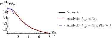
Figure 2: Plot of the d-wave Hall conductivity $\sigma_{\mathrm{DWHE}}$ given by Eq. (12) and Eq. (d-Wave Hall effect and linear magnetoconductivity in metallic collinear antiferromagnets). Values of the parameters used in the numerical calculation are $\frac{h_{x}}{\lambda k_{\mathrm{F}}}=0.25$, $\frac{h_{y}}{\lambda k_{\mathrm{F}}}=0.15$, and $T=0$. We have defined $\sigma_{0}=\left(\frac{1}{2}g\mu_{\mathrm{B}}\right)^{2}\frac{e^{2}\nu_{F}}{\left(\lambda k_{\mathrm{F}}\right)^{2}}$ for brevity.

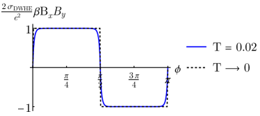
Figure 3: Quantized d-wave Hall effect in insulating system. Insulator is achieved by setting $\frac{k^{2}}{2m}\rightarrow 0$ and $\mu=0$. Plot of the anomalous Hall conductivity $\sigma_{\mathrm{DWHE}}$ as a function of the angle $\phi$ of the in-plane Zeeman magnetic field. Here $h_{x}=h\cos(\phi)$ and $h_{y}=h\sin(\phi)$. Values of the parameters used in the numerical calculation are $h=0.5$, $\mu=0$, $\lambda=0.5$, and $\beta=1.5$.

Let us now briefly mention insulating case. We set $\frac{k^{2}}{2m}\rightarrow 0$ by assuming $m\rightarrow\infty$, and $\mu=0$, then the spectrum (8) becomes $\varepsilon_{\bf k}^{(\pm)}=\pm\sqrt{\Delta_{\bf k}^{2}+\lambda^{2}\tilde{k}^{2}}$. By setting $\mu=0$ the system becomes insulating with a gap equal to $2\sqrt{h_{x}^{2}+h_{y}^{2}}$ at $k_{x}=k_{y}=0$, and to $2\beta\frac{h_{x}h_{y}}{\lambda^{2}}$ at $\tilde{k}_{x}=\tilde{k}_{y}=0$. In Fig. (3) we plot $\sigma_{\mathrm{DWHE}}\beta B_{x}B_{y}$, proportionality coefficient in the right hand side of Eq. (9) between the current and the electric field. Only the valence band contributes at $T=0$ to the current. The conductivity is quantized as $\frac{e^{2}}{2}$, vanishes when either $h_{x}$ or $h_{y}$ is zero, and changes sign in accord with $d-$wave symmetry.

We note that the predicted $d-$wave Hall effect in three-dimensional system will be experimentally measured together with the $\propto({\bf E}\cdot{\bf B}){\bf B}=\left(E_{x}B_{x}+E_{y}B_{y}\right)\left(B_{x}{\bf e}_{x}+B_{y}{\bf e}_{y}\right)$ term in the electric current. In this term it will appear that $B_{x}B_{y}\left(E_{x}{\bf e}_{y}+E_{y}{\bf e}_{x}\right)$ part is looking like the predicted d-wave Hall effect, however, the latter is $\propto\beta B_{x}B_{y}\left(E_{x}{\bf e}_{y}-E_{y}{\bf e}_{x}\right)$, and one will have to filter it out from the former.

Finally, we note that there are other mechanisms contributing to the anomalous Hall effect AHE_RMP ; SinitsynPRB2007 ; NunnerPRB2007 . They are the skew-scattering and side-jump scattering processes due to the impurities, which are expected to alter the amplitude of the predicted here $d-$wave Hall effect but not its symmetry. Their consideration is left for future research.

Let us now discuss linear magnetoconductivity. Although, as we have shown above, integral of the Berry curvature over the angles vanishes when $h_{x}=h_{y}=0$, the Berry curvature can still contribute to the electric current through, for example, modification of the density of states BerryReview . To study the electric current, we employ the method of kinetic equation,

$$\frac{\partial n^{(s)}_{{\bf k}}}{\partial t}+{\dot{\bf k}}^{(s)}\frac{\partial n^{(s)}_{{\bf k}}}{\partial{\bf k}}+{\dot{\bf r}}^{(s)}\frac{\partial n^{(s)}_{{\bf k}}}{\partial{\bf r}}=I_{\mathrm{coll}}[n^{(s)}_{{\bf k}}],$$ (15)

with equations of motion updated in the presence of the Berry curvature BerryReview , ${\dot{\bf r}}^{(s)}=\frac{\partial\epsilon^{(s)}_{{\bf k}}}{\partial{\bf k}}+{\dot{\bf k}}^{(s)}\times{\bf\Omega}^{(s)}_{{\bf k}},$ and ${\dot{\bf k}}^{(s)}=e{\bf E}+\frac{e}{c}{\dot{\bf r}}^{(s)}\times{\bf B}.$ The current is given by ${\bf j}=e\sum_{s=\pm}\int_{\bf k}\left[1+\frac{e}{c}({\bf B}\cdot{\bf\Omega}^{(s)}_{{\bf k}})\right]\dot{{\bf r}}^{(s)}_{\bf k}n^{(s)}_{\bf k}.$ We approximate the kinetic equation only by intra-band scattering, $I_{\mathrm{coll}}[n^{(\pm)}_{{\bf k}}]=({\bar{n}}^{(\pm)}-n^{(\pm)}_{{\bf k}})\tau^{-1},$ where ${\bar{n}}^{(s)}=(4\pi)^{-1}\int\sin(\theta)d\theta d\phi\left[1+\frac{e}{c}({\bf B}\cdot{\bf\Omega}^{(s)}_{{\bf k}})\right]n^{(s)}_{\bf k}$ is the distribution function averaged over the angles, and $\tau$ is the fermion’s life-time due to the elastic scattering on impurities. Inter-band scatterings are also allowed but only by virtue of the spin-orbit coupling $\lambda$, since, without it, the bands are spin polarized and there is no scattering between them. Then these processes will contribute in higher order in spin-orbit coupling than what we will derive. Besides, there is no chiral anomaly in the system and, therefore, inter-band scattering processes are not important.

The kinetic equation is approximated as usual, we follow the lines of ZyuzinWSM ; Zyuzin2021 to obtain for the linear magnetoconductivity defined as ${\bf j}_{\mathrm{LMC}}=\sigma_{\mathrm{LMC}}\beta B_{z}\left(E_{x}{\bf e}_{y}+E_{y}{\bf e}_{x}\right)$, the following expression

$$\sigma_{\mathrm{LMC}}=-2e^{2}\nu_{F}\frac{e\tau}{mc}\frac{k_{\mathrm{F}}}{\sqrt{(2\lambda k_{\mathrm{F}})^{2}+(\beta k_{\mathrm{F}})^{2}}}.$$ (16)

We note that it is the correction to the density of states BerryReview due to the $\frac{e}{c}({\bf B}\cdot{\bf\Omega}^{(s)}_{{\bf k}})$ non-zero product that contributes to this current. In Zyuzin2021 it has been shown that linear magnetoconductivity in ferromagnets can be $\delta{\bf j}=\alpha_{1}({\bf E}\cdot{\bf B}){\bf M}+\alpha_{2}({\bf E}\cdot{\bf M}){\bf B}+\alpha_{3}({\bf M}\cdot{\bf B}){\bf E}$, where Onsager relation requires $\alpha_{1}=\alpha_{2}$ (see also comment comment2 ), whose parts were recently experimentally observed in WSMCorrelated ; LeeRosenbaum2020 ; ExpPRL2021 . Here we found a distinct structure of the linear magnetoconductivity.

We see that the results decay as a power law in the high density limit. On the other hand, antiferromagnetism does not survive extensive doping of the system with conducting electrons. Therefore, our results are expected to be experimentally observed in the low-doping regime of antiferromagnets. We speculate our predicted $d-$wave Hall effect might be relevant to the polar Kerr effect observed in the pseudogap phase of cuprates cuprateEXP . Indeed, either polar Kerr effect or Faraday rotation is due to the off-diagonal elements of the dielectric tensor, which are defined by the Hall effect in the medium. Then the question is which of the anomalous Hall effects, Eq. (1), Eq. (2) or Eq. (3), contributes.

Acknowledgements. We thank I.S. Burmistrov, A.M. Finkel’stein, M.M. Glazov, and A.S. Mel’nikov for helpful discussions. Both authors are supported by the Foundation for the Advancement of Theoretical Physics and Mathematics BASIS. VAZ is grateful to Pirinem School of Theoretical Physics.

References

- (1) R. Karplus and J.M. Luttinger, Phys. Rev. 95, 1154 (1954)
- (2) E.H. Hall, Philos. Mag.10, 301 (1880).
- (3) J. M. Ziman, Electrons and Phonons: The Theory of Transport Phenomena in Solids, (Oxford University Press, Oxford, U.K., 1960).
- (4) F.T. Vas’ko, JETP Lett. 30, 541 (1979); Yu. A. Bychkov and E. I. Rashba, JETP Lett. 39, 78 (1984).
- (5) G. Dresselhaus, Phys. Rev. 100, 580 (1955).
- (6) B. A. Volkov and O. A. Pankratov, Pis’ma Zh. Eksp. Teor. Fiz. 42, 145 (1985) [JETP Lett. 42, 178 (1985)]; O.A. Pankratov, S.V. Pakhomov, and B.A. Volkov, Solid State Communications, 61, 93 (1987).
- (7) Spin Physics in Semiconductors, edited by M. I. Dyakonov (Springer-Verlag, Berlin, Heidelberg, 2008).
- (8) N. Nagaosa, J. Sinova, S. Onoda, A. H. MacDonald, and N. P. Ong, Rev. Mod. Phys. 82, 1539 (2010).
- (9) D. Culcer, A. H. MacDonald, and Q. Niu, Phys. Rev. B 68, 045327 (2003).
- (10) N. A. Sinitsyn, A. H. MacDonald, T. Jungwirth, V. K. Dugaev, and J. Sinova, Phys. Rev. B 75, 045315 (2007).
- (11) T. S. Nunner, N. A. Sinitsyn, M. F. Borunda, V. K. Dugaev, A. A. Kovalev, Ar. Abanov, C. Timm, T. Jungwirth, J. Inoue, A. H. MacDonald, and J. Sinova, Phys. Rev. B 76, 235312 (2007).
- (12) M. Berry, Proc. R. Soc. London, Ser. A 392, 45 (1984).
- (13) D. Xiao, M.C. Chang, and Q. Niu, Rev. Mod. Phys. 82, 1959 (2010).
- (14) A.G. Mal’shukov, K.A. Chao, and M. Willander, Phys. Rev. B 57 2069(R) (1998).
- (15) X. Liu, H.C. Hsu, and C.X. Liu, Phys. Rev. Lett. 111, 086802 (2013).
- (16) J. Zhang, Z. Liu, and J. Wang, Phys. Rev. B 100, 165117 (2019).
- (17) V.A. Zyuzin, Phys. Rev. B 102, 241105(R) (2020).
- (18) J.H. Cullen, P. Bhalla, E. Marcellina, A.R. Hamilton, and Dimitrie Culcer, Phys. Rev. Lett. 126, 256601 (2021).
- (19) T. Kurumaji, arXiv:2304.00785 (2023).
- (20) T. Liang, J. Lin, Q. Gibson, S. Kushwaha, M. Liu, W. Wang, H. Xiong, J.A. Sobota, M. Hashimoto, P.S. Kirchmann, Z.-X. Shen, R.J. Cava, and N.P. Ong, Nature Physics 14, 451 (2018).
- (21) X. Li, J. Koo, Z. Zhu, K. Behnia, and B. Yan, Nature Communications 14, 1642 (2023).
- (22) S.I. Pekar and E.I. Rashba, Sov. Phys. JETP 20, 1295 (1965).
- (23) N.R. Ogg, Proc. Phys. Soc. 89, 431 (1966).
- (24) E.L. Ivchenko and A.A. Kiselev, PTS 26, 1471 (1992).
- (25) C.M. Varma and L. Zhu, Phys. Rev. Lett. 96, 036405 (2006).
- (26) C. Wu, K. Sun, E. Fradkin, and S.-C. Zhang, Phys. Rev. B 75, 115103 (2007).
- (27) S. Hayami, Y. Yanagi, and H. Kusunose, J. Phys. Soc. Jpn. 88, 123702 (2019).
- (28) L.-D. Yuan, Z. Wang, J.-W. Luo, E.I. Rashba, A. Zunger, Phys. Rev. B 102, 144422 (2020).
- (29) S. Hayami, Y. Yanagi, and H. Kusunose, Phys. Rev. B 102, 144441 (2020).
- (30) S.A. Egorov and R.A. Evarestov, J. Phys. Chem. Lett. 12, 2363 (2021).
- (31) L. Šmejkal, J. Sinova, and T. Jungwirth, Phys. Rev. X 12, 031042 (2022);
- (32) L. Šmejkal, J. Sinova, and T. Jungwirth, Phys. Rev. X 12, 040501 (2022).
- (33) A. Bose, N.J. Schreiber, R. Jain, D.-F. Shao, H.P. Nair, J. Sun, X.S. Zhang, D.A. Muller, E.Y. Tsymbal, D.G. Schlom, and D.C. Ralph, Nature Electronics 5, 267 (2022).
- (34) R. González-Hernández, L. Šmejkal, K. Výborný, Y. Yahagi, J. Sinova, T. Jungwirth, and J. Železný, Phys. Rev. Lett. 126, 127701 (2021).
- (35) It has been recently suggested to call such materials as the altermagnets. Here we restrained ourselves from using this name since these materials are primarily collinear antiferromagnets.
- (36) G.F. Koster, J.O. Dimmock, R.G. Wheeler, and H. Statz, Properties of The Thirty-Two Point Groups, MIT Press, Cambridge MA, (1963).
- (37) A. Cortijo, Phys. Rev. B 94, 241105(R) (2016).
- (38) V.A. Zyuzin, Phys. Rev. B 95, 245128 (2017).
- (39) V.A. Zyuzin, Phys. Rev. B 104, L140407 (2021).
- (40) In Zyuzin2021 Onsager reciprocity relation is not satisfied by the terms in the conductivity which are due to the chiral anomaly. Namely, coefficients in Onsager relation dictates , while in Zyuzin2021 . It is possible, side-jump scattering processes has to be included in order to restore the Onsager reciprocity relation, or it might as well be that the relation does not survive the chiral anomaly, when different chemical potentials in the opposite valleys are created thus driving the system out of equilibirum.
- (41) Kuroda, K., Tomita, T., Suzuki, MT. et al., Nature Material 16, 1090 (2017).
- (42) Y. Wang, P.A. Lee, D.M. Silevitch, F. Gomez, S.E. Cooper, Y. Ren, J.-Q. Yan, D. Mandrus, T.F. Rosenbaum, and Y. Feng, Nature Communications 11, 216 (2020).
- (43) B. Jiang, L. Wang, R. Bi, J. Fan, J. Zhao, D. Yu, Z. Li, and X. Wu, Physical Review Letters 126, 236601 (2021).
- (44) V.D. Ky, Sov. Phys. JETP 23, 809 (1966).
- (45) F. Seitz, Phys. Rev. 79, 372 (1950).
- (46) C. Goldman and R.E. Davis, Phys. Rev. 94, 1121 (1954).
- (47) J. Xia, E. Schemm, G. Deutscher, S.A. Kivelson, D.A. Bonn, W.N. Hardy, R. Liang, W. Siemons, G. Koster, M.M. Fejer, and A. Kapitulnik, Phys. Rev. Lett. 100, 127002 (2008).