Analytical investigation of time-dependent two-dimensional non-Newtonian boundary layer equations

Abstract

In this study, five different time-dependent incompressible non-Newtonian boundary layer models in two dimensions are investigated, including external magnetic field effects. The power law, the Casson fluid, the Oldroyd-B model, the Walter fluid B model and the Williamson fluid are analyzed. For the first two models, analytical results are given for the velocity and pressure distributions, which can be expressed by different types of hypergeometric functions. Depending on the parameters involved in the analytical solutions of the nonlinear ordinary differential equation obtained by the similarity transformation, a very wide range of solution types is presented.

I Introduction

The scientific field of classical fluid mechanics is vast and cannot be summarised in a few finite arbitrary books. If we restrict ourselves to non-Newtonian fluids or boundary layer flows, the relevant literature is still remarkably large. The fundamental physics of such fluid flows can be found in basic textbooks such as arista , non-newt , patel schli . In our previous publication on time-dependent self-similar solutions of compressible and incompressible heated boundary layer equations barna-bound , we collected the most relevant literature in the field, which we omit here. Some analytic results are also available for stationary non-Newtonian boundary layers, for example, saer , bog , bog2 , mak .

Today, there is a growing need to study the motion of non-Newtonian fluids, which are often found in industrial applications and in modelling many manufacturing processes (heat exchangers, pharmaceuticals, food, paper). All fluids for which the shear stress-shear rate relation cannot be described by Newton’s law are called non-Newtonian fluids. They can be characterized by formulas of an extremely diverse nature. Without completeness, we will investigate five different non-Newtonian fluid models in our study these are the following: The first is the non-Newtonian power-law model describes the viscosity of time-independent flow behaviour for both shear thinning (or pseudoplastic) and shear thickening (or dilatant) cases (see arista , schli ). This model is used in vast engineering applications, for instance, lubricants, polymers, and slurries yori , this model is well suited for numerical and analytical studies of fluid flows bog , bog2 .

The second can be directly derived from the usual Newtonian fluids. This is the widely used viscosity model for viscoplastic non-Newtonian behaviour and named the Casson fluid model. Fluids that behave like a solid when the shear stress is less than the yield stress applied to a liquid, and start to deform when the shear stress is greater than the yield stress casson .

Our third model is the non-Newtonian Oldroyd-B fluid is used in the literature for the rheological characterization of a type of viscoelastic fluid. Oldroyd applied the principle that stresses in a continuous medium can only arise from deformations and cannot change if the material is only rotated old .

The fourth is the Walters-B model which was proposed by Walters for viscoelastic fluids walt . It is a generalisation of the Oldroyd-B model and is used to describe the behaviour of fluids that are mainly used in food and food processing technologies.

The final model is the Williamson fluid model which can also be used to describe the viscoelastic shear thinning properties of non-Newtonian fluids wil . In Williamson’s fluid model, the effective viscosity should decrease infinitely as the shear rate increases, which is effectively infinite viscosity at rest (no fluid motion) and zero viscosity as the shear rate approaches infinity.

The actual existing literature on non-Newtonian boundary layers is enormous, therefore we cannot give a general overview just mention some relevant recent publications in the right place in this study.

To analyse the variation in flow characteristics of a fluid in a magnetic field, an additional magnetic term is added to the momentum equation of the boundary layer equation system, so that the boundary layer equation system can describe the magnetic effects.

The aim of this paper is to provide analytic results for the stationary equations of the non-Newtonian fluid flows in a magnetic field. The above given five types of non-Newtonian behaviour are examined. The governing equations are transformed into a system of ordinary differential equations by a similarity transformation. We analyze the cases in which the fluid flow rate functions can be analytically given by the method used. In these two cases, we give the velocity distributions in two space dimensions and point out the effect of each parameter.

II Mathematical models

II.1 Power-law viscosity

For power-law viscosity, our partial differential equation system systems reads as follows:

$$\frac{\partial u}{\partial x}+\frac{\partial v}{\partial y} = 0,$$ (1)

$$\rho\left(\frac{\partial u}{\partial t}+u\frac{\partial u}{\partial x}+v\frac{\partial u}{\partial y}\right) = -\frac{\partial p}{\partial x}+m\frac{\partial}{\partial y}\left(\left|\frac{\partial u}{\partial y}\right|^{n-1}\cdot\frac{\partial u}{\partial y}\right)+\sigma B_{0}^{2}u,$$ (2)

$$\frac{\partial p}{\partial y} = 0,$$ (3)

where the dynamical variables are the velocities components $u(x,y,t),v(x,y,t)$, the fluid pressure $p(x,y,t)$, $B_{0}=const$ is the magnetic the magnetic induction, and $\sigma$ is the electrical conductivity. Additional physical parameters are $\rho,m,n$ the fluid density, consistency parameter, and the power-law index, respectively. To fix the geometrical relations in our system consider Fig.(1).

The temporal decay of the strong solutions of the power-law type of non-Newtonian fluids for variable power-law index was mathematically proven by Ko power1 . Flow reversal effects in an expanding channel for this type of viscous fluid were analyzed by power2 . A non-iterative transformation method to an extended Blasius problem describing a 2D laminar boundary-layer with power-law viscosity for non-Newtonian fluids was developed by Fazio power3 . The stationary power-law equations were solved by Pater et al. patel by the one-parameter deductive group theory technique. (We have to mention at this point that the stationary boundary layer equations can be reduced to the third-order non-linear differential equation which is called the Blasius equation having an extensive literature which we skip now.)

To obtain the solutions to the system (1)-(3), we apply the following self-similar Ansatz for $u,v$ and $p$:

$$u(x,y,t)=t^{-\alpha}f(\eta),\hskip 28.45274ptv(x,y,t)=t^{-\delta}g(\eta),\hskip 28.45274ptp(x,y,t)=t^{-\gamma}h(\eta),$$ (4)

with the argument $\eta=\frac{x+y}{t^{\beta}}$ of the shape functions. All the exponents $\alpha,\beta,\gamma,\delta$ are real numbers. Solutions with integer exponents are called self-similar solutions of the first kind, non-integer exponents generate self-similar solutions of the second kind sedov .

It is necessary to remark that, the heat conduction mechanism to (1) - (3) the boundary layer equations can exclude the self-similarity using transformation (4) one gets contradiction among self-similar exponents.

The shape functions $f,g$ and $h$ could be any arbitrary continuous functions with existing first and second continuous derivatives and will be derived later on. The physical and geometrical interpretation of the Ansatz were exhaustively analyzed in former publications imre1 ; imre3 , therefore we skip it here.

The main points are, that $\alpha,\delta,\gamma$ are responsible for the rate of decay and $\beta$ is for the rate of spreading of the corresponding dynamical variable for positive exponents. Negative exponents mean physically irrelevant cases, blowing up and contracting solutions. The numerical values of the exponents are considered as follows:

$$\alpha=\delta=n/2,\hskip 28.45274pt\beta=1-\alpha=1-n/2,\hskip 28.45274pt\gamma=n.$$ (5)

Exponents with numerical values of one-half mean the regular Fourier heat conduction (or Fick’s diffusion) process. One-half values for the exponent of the velocity components and unit value exponent for the pressure decay are usual for the incompressible Navier-Stokes equation imre4 . Note, that the value of $\gamma$ is responsible for the decay of the pressure field. °

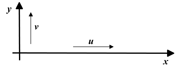
Figure 1: Defining the directions and the velocity components of the investigated system.

Applying (5), the derived ordinary differential equation (ODE) system reads as

$$f^{\prime}+g^{\prime}=0,$$ (6)

$$\rho\left(-\frac{n}{2}f-\left[1-\frac{n}{2}\right]\eta f^{\prime}+ff^{\prime}+gf^{\prime}\right)=-h^{\prime}+mnf^{\prime\prime}|f^{\prime}|^{n-1}+\sigma B_{0}^{2}f,$$ (7)

$$h^{\prime}=0,$$ (8)

where the prime means derivation concerning variable $\eta$. Equations (6) and (8) can be integrated, to get $f+g=c_{1}$ and $h=c_{2}$. However, the dynamic variable under consideration is the velocity component $u$, which is $f$. From (7) the derived ODE is the following:

$$\frac{mn}{\rho}f^{\prime\prime}|f^{\prime}|^{n-1}+\left(\left[1-\frac{n}{2}\right]\eta-c_{1}\right)f^{\prime}+Kf=0,$$ (9)

where $K=(\rho n/2+\sigma B_{0}^{2}).$ The constant $c_{1}$ can be determined from possible boundary conditions applied to the fluid flow problem.

Here, we give analytic and numeric solutions to the flow (6)-(8).

i.) First we consider the case $B_{0}=0$. Equation (9) has analytic solutions only for the cases of $n=1,0$ and $-1$.

For the Newtonian fluid case, when $n=1$, and other parameters ($c_{1},m,\rho$) are general, the solution reads as

$$f(\eta)=C_{1}M\left(\frac{\rho}{2},\frac{1}{2},-\frac{\rho(\eta-2c_{1})^{2}}{4m}\right)+C_{2}U\left(\frac{\rho}{2},\frac{1}{2},-\frac{\rho(\eta-2c_{1})^{2}}{4m}\right),$$ (10)

where $M(,,)$ and $U(,,)$ are the Kummer M and U functions NIST and $C_{1}$ and $C_{2}$ stand for the usual integration constants. The parameter $c_{1}$ just shifts the maxima of the shape function and $m$ the consistency parameter (which is positive) just changes the full width at half the maximum of the function. The larger the numerical value of $m$ the broader the shape function. The third parameter, the density of the fluid (which must be also positive) is the most relevant parameter of the flow which of course, meets our physical intuition. Figure (2) shows four different velocity shape functions for different fluid densities. It is important to mention that for density $0<\rho$ the shape function has a global maxima in the origin and a decay to zero, (larger densities mean quicker decay.) however for $1<\rho$ the shape function shows additional oscillations as well. The final velocity field has the asymptotic form of $u(x,y=0,t)=t^{-\frac{1}{2}}f\left(\frac{x}{t^{1/2}}\right)$. For completeness, we give the entire formula for $u$ as well:

$$u(x,y,t)=\frac{1}{t^{1/2}}\left(C_{1}M\left[\frac{\rho}{2},\frac{1}{2},-\frac{\rho\left\{\frac{(x+y)}{t^{1/2}}-2c_{1}\right\}^{2}}{4m}\right]+C_{2}U\left[\frac{\rho}{2},\frac{1}{2},-\frac{\rho\left\{\frac{(x+y)}{t^{1/2}}-2c_{1}\right\}^{2}}{4m}\right]\right).$$ (11)

We remark that this case was investigated in barna-bound . Figure (3) shows the velocity field of $v(x,y=0,t)$ for a parameter set. The slight oscillation and the quick decay are clear to see. It is interesting to mention here, that during our investigations using the self-similar Ansatz, we regularly get solutions which contain Kummer’s function for hydrodynamic processes like the Bénard-Rayleigh convection imre1 or even for regular diffusion equation laci_roman .

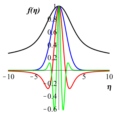
Figure 2: Four different velocity shape functions for Eq. (10). The black, blue, red and green curves are for $\rho=0.5,1,2$ and $5$, respectively. All additional parameters are the same for all four curves ($C_{1}=1,C_{2}=0,c_{1}=0$ and $m=2$ ).

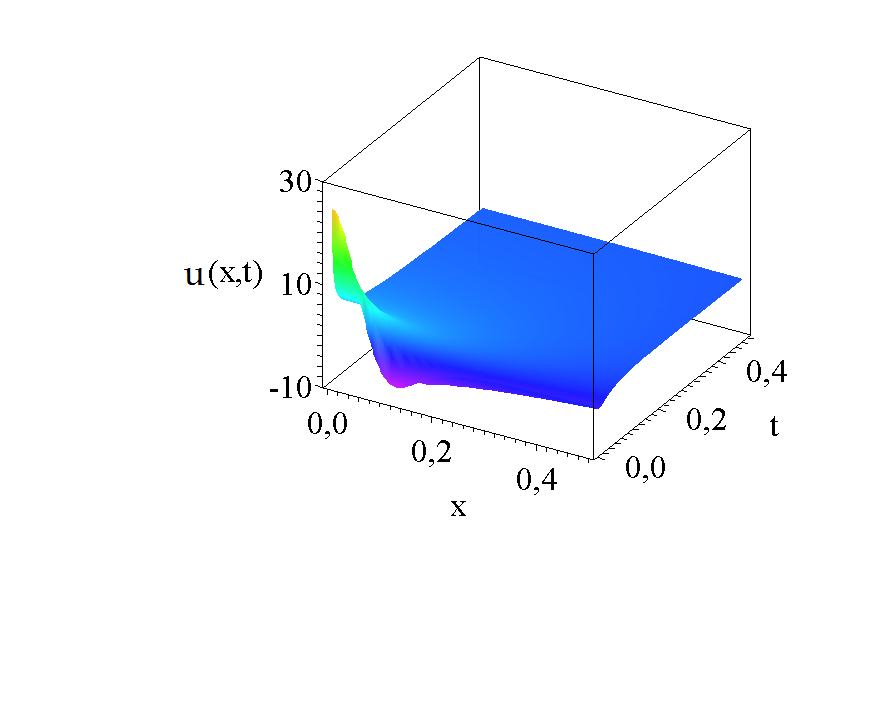
Figure 3: The velocity distribution function projection for $y=0$ for the density of $\rho=2$. All other parameters are the same as below.

For the case $n=K=0$ the solution is a trivial constant $f=c_{2}$.

There are analytic solutions available for $n=-1$ unfortunately, not for the general case where all the other three parameters $(c_{1},\rho,m)$ are completely free. The constant $c_{1}$ should be equal to zero and the ratio of $\rho/m$ should have some special values. The existing possibilities are not so many.

In the following we present some solutions which came from our numerical experimental experiences:
For $\rho=1$ and for arbitrary integer or rational m we get the next implicit relation for the solutions:

$$ln(\eta)-ln(f[\eta])-ln\left(C_{1}U\left[-1,\frac{3}{2},\frac{1}{4m}f\{\eta\}^{2}\right]+M\left[-1,\frac{3}{2},\frac{1}{4m}f\{\eta\}^{2}\right]\right)-C_{2}=0.$$ (12)

If the first parameters of the Kummer’s functions are non-positive integers the series becomes finite

$$M\left[-1,\frac{3}{2},\frac{1}{4m}f\{\eta\}^{2}\right]=1-\frac{2}{3m}f(\eta)^{2},$$

$$U\left[-1,\frac{3}{2},\frac{1}{4m}f\{\eta\}^{2}\right]=-\frac{3}{2}+\frac{1}{m}f(\eta)^{2},$$ (13)

considering that $C_{2}>0$ and $\tilde{C_{2}}=ln({C_{2}})$ after some trivial algebraic steps we get:

$$\left(\frac{\tilde{C}_{2}C_{1}}{m}-\frac{2\tilde{C}_{2}}{m}\right)f(\eta)^{3}+\left(\tilde{C}_{2}-\frac{3\tilde{C}_{2}C_{1}}{2}\right)f(\eta)-\eta=0.$$ (14)

The velocity shape functions can be seen in figure 4.

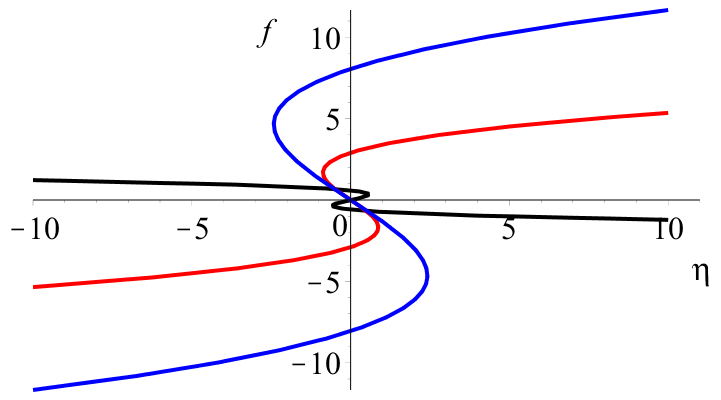
Figure 4: The implicit velocity shape functions of Eq. (14) for three different parameter sets $(C_{1},\tilde{C}_{2},m)$. The black, red and blue curves are for $(1,4,0.4)$, $(2.4,0.3,1.3)$ and $(2.4,0.3,10)$ .

One can see on Eq. (14), that if $\eta=0$, than $f(\eta=0)=0$ is a solution of the equation. Further possibilities gives the following rearrangement

$$\left[\left(\frac{\tilde{C}_{2}C_{1}}{m}-\frac{2\tilde{C}_{2}}{m}\right)f(\eta)^{2}+\left(\tilde{C}_{2}-\frac{3\tilde{C}_{2}C_{1}}{2}\right)\right]f(\eta)=0.$$ (15)

This yields

$$f(\eta=0)=\pm\sqrt{\left(\frac{3\tilde{C}_{2}C_{1}}{2}-\tilde{C}_{2}\right)/\left(\frac{\tilde{C}_{2}C_{1}}{m}-\frac{2\tilde{C}_{2}}{m}\right)}.$$ (16)

It shows that for $\eta=0$ there is one or there are three corresponding values to function $f(\eta)$. In the following we try to find the constraints on the parameters which separate the two cases. If we consider the inverse function $f(\eta)=y$, we have

$$\eta=\left(\frac{\tilde{C}_{2}C_{1}}{m}-\frac{2\tilde{C}_{2}}{m}\right)\cdot y^{3}+\left(\tilde{C}_{2}-\frac{3\tilde{C}_{2}C_{1}}{2}\right)\cdot y.$$ (17)

The derivative of this function is

$$\frac{d\eta}{dy}=3\left(\frac{\tilde{C}_{2}C_{1}}{m}-\frac{2\tilde{C}_{2}}{m}\right)\cdot y^{2}+\left(\tilde{C}_{2}-\frac{3\tilde{C}_{2}C_{1}}{2}\right).$$ (18)

If this expression has always the same sign, the function is monotonous, and then there is just one single root $\eta(y=0)=0$ (i.e. $f(\eta=0)=0$). If this derivative may change the sign, then multiple roots are possible. The inverse function is not monotonous and may have three roots if there are real roots of the equation of derivative $d\eta/dy=0$. This means the following condition

$$\frac{\left(\frac{3\tilde{C}_{2}C_{1}}{2}-\tilde{C}_{2}\right)}{\left(\frac{\tilde{C}_{2}C_{1}}{m}-\frac{2\tilde{C}_{2}}{m}\right)}>0.$$ (19)

Figure (4) shows two implicit solutions of Eq. (14) for three different parameter sets. Note, that Eq.(14) is a third-order equation we may get multi-valued solutions. If the parameter $m$ is much smaller than the two integration constants then single-valued solutions emerge as well. Whether the multi-valued solutions have any physical significance is not yet clear, but it is thought that this property may indicate the existence of finite oscillations or eddies. Figure (5) shows the projected velocity fields $(y=0)$ for single and double-valued case. (For a better visibility we present the solution function from an unusual perspective.) The decrease of the velocity field with time is clearly visible. For the sake of completeness, we give the final form of the velocity field, which reads:

$$\left(\frac{\tilde{C}_{2}C_{1}}{m}-\frac{2\tilde{C}_{2}}{m}\right)t^{3/2}f\left(\frac{(x+y)}{t^{3/2}}\right)^{3}+\left(\tilde{C}_{2}-\frac{3\tilde{C}_{2}C_{1}}{2}\right)t^{1/2}f\left(\frac{(x+y)}{t^{3/2}}\right)-\frac{(x+y)}{t^{3/2}}=0.$$ (20)

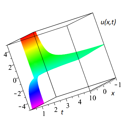
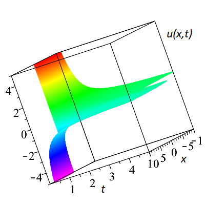
a)                            b)

Figure 5: The implicit velocity distribution $u(x,t)$ evaluated from Eq. (21) for two different parameter sets a) figure is for $(1,4,0.4)$ and b) figure is for $(0,2.5,0.7)$, respectively.

There are analytic solutions available for $\rho=3$ and for arbitrary real $m$ and $c_{1}$ in the implicit form of:

$$\frac{\eta}{f(\eta)}+\frac{C_{1}e^{\frac{9f(\eta)^{2}}{4m}}}{3f(\eta)}-\frac{C_{1}\cdot erf\left(\frac{3}{2}\sqrt{-\frac{1}{m}}f[\eta]\right)}{2m\sqrt{-\frac{1}{m\pi}}}-\frac{2c_{1}}{3f(\eta)}-C_{2}=0.$$ (21)

Equation (21) clearly shows, that for $C_{1}=0$, we get the trivial linear function as a solution. Figure (6) presents the solutions of Eq. (21) for two parameter sets. Because of the quadratic appearance of $f(\eta)$, we obtain dual-valued curves which are not strictly speaking functions. The result functions increase strongly (or decrease in the case of a negative branch) very close to the origin and for larger arguments on a nearly horizontal plateau. The general structure of the solution is quite stable, even a tenfold change in the parameters does not change the overall feature of the derived curve. To have a better overview of the properties of the solution, Figure (7) presents the usual velocity projection of $u(x,y=0,t)$ for a given parameter set. The physically relevant rapid decay over time is again clearly visible.

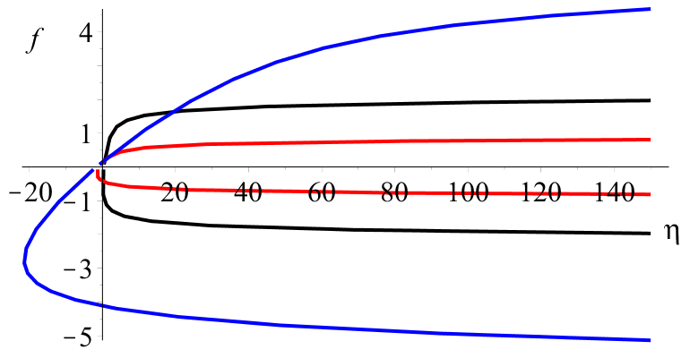
Figure 6: The implicit velocity shape functions of Eq.(21) for three different parameter sets $(C_{1},\tilde{C}_{2},c_{1},m)$ with $\rho=3$. The black, red and blue curves are for $(1,1,1,0,1)$, $(3,5,0,0,0.2)$ and $(13,11,4,10)$, respectively

.

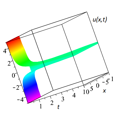
Figure 7: The implicit velocity distribution field when the parameters are $\rho=3$, $(C_{1},\tilde{C}_{2},c_{1},m)$ and $(3,5,0,0.2)$ with $\rho=3$.

ii.) In the second part of our analysis, we investigate the solutions when the magnetic induction is not equal to zero ($B_{0}\neq 0$). Even now four different cases exist $n=2,1,\ 0$ and $-1$. We have to examine them one by one.

First, we consider the dilatant case $n=2$. Equation (9) is reduced to

$$\frac{2m}{\rho}f^{\prime\prime}f^{\prime}+Kf=0.$$ (22)

multiplying by $f^{\prime}$ we get a total derivative which can be integrated giving us the ODE of:

$$\frac{2m}{3\rho}f^{\prime 3}+\frac{1}{2}(\rho+\sigma B_{0}^{2})f"+c_{0}=0.$$ (23)

First considering the $c_{0}=0$ simpler case, the ODE can be directly integrated and gives multiple solutions: there is a trivial one of $f=0$ there are two complex conjugated solutions which we skip and a relevant real one. After some algebraic manipulation, it reads as:

$$f=-\frac{6\rho(\rho+\sigma B_{0}^{2})(\eta-c_{1})^{3}}{216\cdot m},$$ (24)

which is a third-order parabola in the variable of $\eta$. The final velocity distribution is

$$u(x,y,t)=-\frac{6\rho(\rho+\sigma B_{0}^{2})(x+y-c_{1})^{3}}{216\cdot m\cdot t},$$ (25)

which is divergent at $t=0$ for large spacial coordinates and has quick $t^{-1}$ decay in time in general. Figure (8) shows the graph of Eq. (25) for a given parameter set.

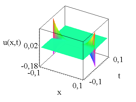
Figure 8: The projection of Eq. (25) $u(x,y=0,t)$ for the parameter set of $(\rho,m,\sigma,B_{0},c_{1})$ equal to $(1,0.1,1,0)$, respectively.

For $c_{0}\neq 0$, there is a formal implicit solution containing an integral:

$$\eta-\int^{f(\eta)}\frac{2m}{[-6\rho m^{2}(a^{2}{\rho+a^{2}\sigma B_{0}^{2}+2c_{0}})]^{1/3}}da-c_{1}=0.$$ (26)

Unfortunately, for general arbitrary parameters $(\rho,m,\sigma,B_{0}^{2},c_{0})$ it cannot be evaluated.

The second case is $n=1,$ the Newtonian fluid case:

$$f(\eta)=C_{1}\cdot M\left(\frac{\rho}{2}+\sigma B_{0}^{2},\frac{1}{2},-\frac{\rho[\eta-2c_{1}]^{2}}{4m}\right)+C_{2}\cdot U\left(\frac{\rho}{2}+\sigma B_{0}^{2},\frac{1}{2},-\frac{\rho[\eta-2c_{1}]^{2}}{4m}\right).$$ (27)

Note, the interesting feature that both the density and the magnetic induction give contributions into the first parameter of Kummer’s functions. The density $\rho$ and the square of the magnetic induction $B_{0}^{2}$ are always positive the electric conductivity $\sigma$ is also positive for regular materials. (With the need for completeness we have to note that there are so-called metamaterials which can have negative electrical conductivity but we skip that case now. More on materials can be found in meta . For such media the first parameter of Kummer’s function would be negative which would mean divergent velocity fields, which contradicts energy conservation.) For regular materials, the external magnetic field enhances the first positive parameter of Kummer’s functions which means more oscillations and quicker decay. The shape function or the final velocity distribution $u(x,y,t)$ is very similar which was presented in Fig.(2) and Fig.(3). If the first parameter of Kummer’s M function $(\rho/2+\sigma B_{0}^{2})$ is larger than one then the larger the magnetic induction the larger the number of oscillations. This is true for the density and for the electric conductivity as well. Such shape functions are presented in fig (9).

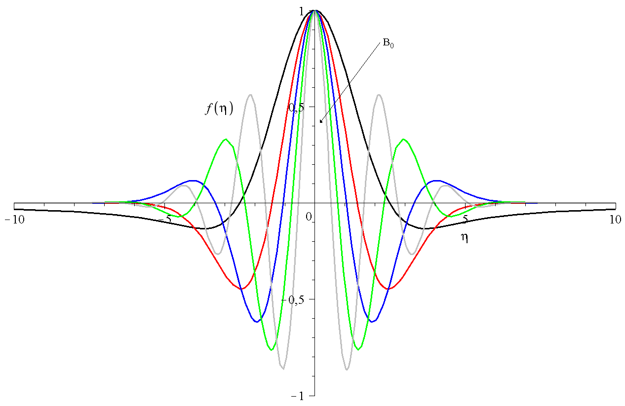
Figure 9: Five shape functions of Eq. (27) for different parameter sets. The effect of the magnetic induction is investigated. The black, red, blue and green lines are for $(C_{1},C_{2},c_{1},\rho,m,\sigma,B_{0}^{2})$ with numerical values of $(1,0,0,1,1,1,0.1)$, $(1,0,0,1,1,1,0.5)$, $(1,0,0,1,1,1,1)$, $(1,0,0,1,1,1,2)$, and $(1,0,0,1,1,1,4)$, respectively

.

The third case is $n=0$ which is the simplest one. The original ODE of Eq. (9) is reduced to

$$\eta f^{\prime}+\sigma B_{0}^{2}f=0,$$ (28)

with the trivial solution of:

$$f(\eta)=C_{1}\eta^{-\sigma B_{0}^{2}}.$$ (29)

The velocity distribution has the form

$$u(x,y,t)=C_{1}\left(\frac{(x+y)}{t}\right)^{-\sigma B_{0}^{2}}.$$ (30)

The pressure field is a pure constant as well. These are simple power laws, therefore, we skip to present additional figures.

The last case, $n=-1$, is again the most complicated one. There is no analytic solution available when all parameters are arbitrary. There is however a special case when the last term in Eq. (9) is zero which defines the constraint of $\rho=2\sigma B_{0}^{2}$. If we additionally fix $c_{1}=0$ we get the following solution:

$$f(\eta)=\pm\frac{{1}}{3}\sqrt{\frac{6m}{3\rho}}\cdot arctan\left(\frac{\sqrt{6m\rho}\eta}{\sqrt{-6m\rho\eta^{2}+2mC_{1}}}\right)+C_{2}.$$ (31)

It can be easily shown that the solution has a compact support, and the function is only defined in the region of $-\sqrt{\frac{C_{1}}{3\rho}}\leq\eta\leq\sqrt{\frac{C_{1}}{3\rho}}$. Note, that the smaller the fluid density the larger the acceptable velocity range if $c_{1}$ remains the same. The larger the integral constant $c_{1}$ parameter the larger the available velocity range. The second integral constant $C_{2}$ just shifts the solution parallel to the $y$ axis. Figure (10) shows the solution for three different parameter sets. Figure (11) presents the final typical velocity distribution $v(x,y=0,t)\sim t^{\frac{1}{2}}f(\frac{x}{t^{3/2}})$ the quick temporal decay is clear to see. Note, that the prefactor $t^{\frac{1}{2}}$ makes the time backpropagation impossible for negative values.

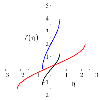
Figure 10: The velocity shape functions of Eq. (31) for three different parameter sets $(C_{1},C_{2},m,\rho)$ with $c_{1}=0$. The black, red and blue curves are for $(1,0,1,1),(15,0.2,2,1)$ and $(0.4,2,1,0.4)$, respectively

.

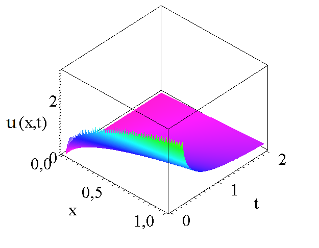
Figure 11: The velocity distribution which corresponds to (31) for the parameter set $(C_{1},C_{2},\rho,m)$ is $(0,0,5,3)$

.

For the sake of completeness, we give the solutions for the pressure as well. The ODE of the shape function is trivial with the solution of:

$$h^{\prime}=0,\hskip 28.45274pth=c_{2}.$$ (32)

Therefore, the final pressure distribution reads:

$$p(x,y,t)=t^{-\gamma}\cdot h(x,y,t)=\frac{c_{2}}{t^{n}},$$ (33)

which means that the pressure is constant in the entire space at a given time, and the time decay can be different to the velocity field.

II.2 Casson fluid

To perform an even more comprehensive analysis to study how the transients happen in non-Newtonian boundary layers we investigated additional fluid models.

The first in our line is the simplest one, the so-called Casson fluid model, now the boundary layer equation has the form of

$$\rho\left(\frac{\partial u}{\partial t}+u\frac{\partial u}{\partial x}+v\frac{\partial u}{\partial y}\right)=-\frac{\partial p}{\partial x}+\left(1+\frac{1}{\lambda}\right)\mu\frac{\partial^{2}u}{\partial x^{2}}+\sigma B_{0}^{2}u,$$ (34)

where $\lambda$ is the Casson parameter. Note that for $\lambda\rightarrow\infty$ the term goes over the regular Newtonian viscous term. (All five physical parameters $\rho,\lambda,\mu,B_{0}$ and $\sigma$ should should have positive real values and the $\lambda\neq 0$ is also evident.) The variational approach for the flow of Casson fluids in pipes was analyzed by Sochi sochi . The blood flow through a stenotic tube was modelled by the Casson fluid by Tandon et al. tandon .

We still consider the self-similar Ansatz of (4) for the three dynamical variables. After the usual algebraic manipulations, we arrive at the non-linear second-order ODE for the shape function of horizontal velocity component $f(\eta)$ in the next form:

$$\rho\left(-\frac{f}{2}-\frac{\eta f^{\prime}}{2}\right)=\left(1+\frac{1}{\lambda}\right)\mu f^{\prime\prime}+\sigma B_{0}^{2}f,$$ (35)

in this model, all four self-similar exponents have fixed values, $\alpha=\beta=\delta=1/2,\gamma=1$, which is usual for the Newtonian viscous fluid equations imre4 . The derived solutions are mainly different to the first model, therefore we have to give a detailed analysis in the following. With our usual mathematical program package Maple 12, we can easily derive the solution in closed form:

$$f(\eta)=e^{-\frac{\rho\eta^{2}}{4\mu\left(\frac{\lambda+1}{\lambda}\right)}}\cdot\eta\cdot\left(C_{1}M\left[-\frac{2\sigma B_{0}^{2}-\rho}{2\rho},\frac{3}{2},\frac{\rho\eta^{2}}{4\mu\left\{\frac{\lambda+1}{\lambda}\right\}}\right]\right.+$$

$$\left.C_{2}U\left[-\frac{2\sigma B_{0}^{2}-\rho}{2\rho},\frac{3}{2},\frac{\rho\eta^{2}}{4\mu\left\{\frac{\lambda+1}{\lambda}\right\}}\right]\right).$$ (36)

It is important to note at this point, that the derived formula shows some similarities to the results of the regular diffusion equations laci_roman which was exhaustively discussed in our former studies. The situation is however a bit different here. Thanks to the positivity of all parameters, the sign of exponent is always negative (which is a real Gaussian function) which dictates a rapid decay for large arguments $\eta$ and for any kind of additional parameter sets. The crucial parameter which qualitatively classifies the solutions is the numerical value of the first parameter of Kummer’s functions. We can distinguish three cases:

• $-\left(\frac{2\sigma B_{0}^{2}-\rho}{2\rho}\right)<0$ which is equivalent to $2\sigma B_{0}^{2}>\rho$ (with the stipulation of $\rho\neq 0$) the solutions have oscillations. If this parameter is a negative integer the infinite series of the Kummer’s function breaks down to a finite order polynomial. The smaller the parameter the larger the number of oscillations.

• $-\left(\frac{2\sigma B_{0}^{2}-\rho}{2\rho}\right)=0$ which is equivalent to $2\sigma B_{0}^{2}=\rho$ (with the stipulation of $\rho\neq 0$) now both Kummer’s M and Kummer’s U functions are unity and the solution is reduced to the Gaussian function times $\eta$ function which has odd symmetry. This is the limiting solution between the oscillating and the non-oscillating solutions.

• $-\left(\frac{2\sigma B_{0}^{2}-\rho}{2\rho}\right)>0$ which is equivalent to $2\sigma B_{0}^{2}<\rho$ (with the stipulation of $\rho\neq 0$) the larger the parameter the smaller peak value of the solution and the quicker the decay.

Figure (12) presents five shape functions of Eq. (36) for five different fluid densities, for a clear comparison all the other parameters remain the same. The larger the density $\rho$ the quicker the decay and the smaller the global maximum of the shape functions.

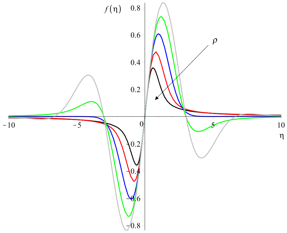
Figure 12: Five shape functions of Eq. (36) for different parameter sets. The role of the fluid density $\rho$ is investigated. The black, red, blue green and grey lines are for $(C_{1},C_{2},\rho,\lambda,\mu,\sigma,B_{0}^{2})$ with numerical values of $(1,0,8,1,1,1,1),(1,0,4,1,1,1,1),(1,0,2,1,1,1,1),(1,0,1,1,1,1,1)$ and $(1,0,1/2,1,1,1,1)$, respectively

.

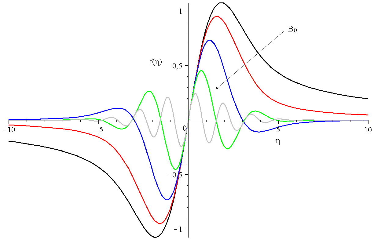
Figure 13: Five shape functions of Eq. (36) for different parameter sets. The role of the magnetic induction $B_{0}^{2}$is investigated. The black, red, blue and green lines are for $(C_{1},C_{2},\rho,\lambda,\mu,\sigma,B_{0}^{2})$ with numerical values of $(1,0,1,1,1,1,0.1),(1,0,1,1,1,1,0.5),(1,0,1,1,1,1,1),(1,0,1,1,1,1,2)$ and $(1,0,1,1,1,1,4)$ respectively

.

In general, the ${\rho}/[{4\mu(\lambda+1)/\lambda]}$ factor is responsible for the extent (or the full with at half maximum (FWHM) value of the solution) the larger this parameter the quicker the decay. For changing the Casson parameter in the physically relevant positive range $\lambda>0$ we found no remarkable change in the solutions, this is because the $\frac{\lambda+1}{\lambda}$ (is almost unit) factor appears in the Gaussian together with two other parameters.

The role of the magnetic induction is also important to know. Figure (13) shows the effect of the magnetic induction $B_{0}^{2}$ where all the other parameters and unchanged. If the first parameter of Kummer’s M function is smaller than unity the solutions has a global maxima and a quick decay, if this parameter is larger than the unity then the larger the magnetic induction the larger the oscillations of the solutions.

Most of these solutions have odd symmetry. It can be easily seen because the Gaussian is an even function $\eta$ is an odd function and the series of Kummer’s M and U functions which have a quadratic argument are again even infinite or finite series which together given odd symmetry. However, using the series expansion it can be shown that if the first parameter of the Kummer’s U (only for U ) function $-\left(\frac{2\sigma B_{0}^{2}-\rho}{2\rho}\right)$ is a negative half-integer then the solutions get even symmetry. The properties of such kinds of solutions are exhaustively discussed in laci .

To complete our analysis we give the solutions for the pressure as well. The ODE of the shape function is trivial with the solution of:

$$h^{\prime}=0,\hskip 28.45274pth=c_{2}.$$ (37)

Therefore, the final pressure distribution is:

$$p(x,y,t)=t^{-1}\cdot h(x,y,t)=\frac{c_{2}}{t^{-1}},$$ (38)

which means that the pressure is constant in the entire space at a given time, and the temporal decay follows the simple inverse law.

II.3 Oldroyd-B model

The next fluid flow model is the Oldroyd-B model old , where the momentum equation is the following:

$$\frac{\partial u}{\partial t}+u\frac{\partial u}{\partial x}+v\frac{\partial v}{\partial y}+\frac{\lambda_{1}}{\rho}\left(u^{2}\frac{\partial^{2}u}{\partial x^{2}}+2uv\frac{\partial^{2}u}{\partial x\partial y}+v^{2}\frac{\partial^{2}u}{\partial y^{2}}\right)=-\frac{1}{\rho}\frac{\partial p}{\partial x}+\frac{\nu}{\rho}\frac{\partial^{2}u}{\partial y^{2}}$$

$$+\frac{\nu\lambda_{2}}{\rho}\left(u\frac{\partial^{3}u}{\partial x\partial y^{2}}+v\frac{\partial^{3}u}{\partial y^{3}}-\frac{\partial u}{\partial y}\frac{\partial^{2}u}{\partial y^{2}}-\frac{\partial u}{\partial y}\frac{\partial^{2}v}{\partial y^{2}}\right)+\sigma B_{0}^{2}u.$$ (39)

Even without the external term with the magnetic induction, the self-similar Ansatz of (4) leads to contradiction among the four self-similar exponents indicating that the system has no self-similar symmetry with power-law time decay. The main cause of the lack of symmetry is the appearance of the third spatial derivatives together with the second ones. The Oldroyd-B model was exhaustively investigated in the last decades from many points of views, optimal time decay rates for the higher order spatial derivatives of solutions were analysed by Wang wang . The global wellposedness of the model was investigated by Elgindi and Liu elg . The global existence results of some Oldroyd-B models were proven by hieber . Finally, we mention the review paper of rev which summarizes most of the known mathematical results.

II.4 Walters’ Liquid B model

The third possible non-Newtonian candidate is the so-called Walters’ Liquid B model, walt where the momentum equation has the form of:

$$\frac{\partial u}{\partial t}+u\frac{\partial u}{\partial x}+v\frac{\partial v}{\partial y}=-\frac{1}{\rho}\frac{\partial p}{\partial x}+\frac{\mu}{\rho}\frac{\partial^{2}u}{\partial y^{2}}+\frac{k_{0}}{\rho}\left(u\frac{\partial^{3}u}{\partial x\partial y^{2}}+v\frac{\partial^{3}u}{\partial y^{3}}-\frac{\partial u}{\partial y}\frac{\partial^{2}u}{\partial x\partial y}+\frac{\partial u}{\partial x}\frac{\partial^{2}u}{\partial y^{2}}\right)+\sigma B_{0}^{2}u.$$ (40)

Practically, we observed the same as in the previous case, the existence of the terms with the third derivatives destroyed the self-similar symmetry therefore no solutions can be derived.

Flow and heat transfer of Walter’s liquid model with stretching walls were applied to haemodynamics by Misra, Shit and Rath mis . Khrisna kris studied the Hall and ion slip effects on MHD laminar flow of in a Walter’s‐B fluid.

II.5 Williamson fluid

In the last model, we took the Williamson fluid wil with the equation of motion of:

$$\frac{\partial u}{\partial t}+u\frac{\partial u}{\partial x}+v\frac{\partial v}{\partial y}=-\frac{1}{\rho}\frac{\partial p}{\partial x}+\frac{\partial}{\partial y}\left(\frac{\mu}{\rho}\frac{\partial u}{\partial y}+\mu\frac{\Gamma}{2}\left(\frac{\partial u}{\partial y}\right)^{2}\right)+\sigma B_{0}^{2}u.$$ (41)

Even if this model lacks the property of time-dependent self-similar symmetry, therefore we cannot present analytical results. Malik, et al. malik however numerically studied the effects of variable thermal conductivity and heat generation/absorption on Williamson fluid flow and heat transfer. The swimming effects of microbes in blood flow of nano-bioconvective Williamson’s fluid was investigated by Rana et all. rana . We found these recent results which we think are worth mentioning.

III Summary and Outlook

In our study, we investigated five different time-dependent non-Newtonian boundary layer problems using the self-similar approach. We show that analytical results exist and give them. For the non-Newtonian power-law fluid, we found different types of solutions depending on the value of the power-law exponent, which can be expressed by Kummer functions or other implicit functions. The effects of density and other parameters in the nonlinear ordinary differential equation have been investigated. The effects of the magnetic field can be described by including an additional magnetic term in the equation. Analytical solutions have also been found for such cases. For non-Newtonian Casson fluid flow, the effect of the Casson parameter is also analyzed. For the other three non-Newtonian cases, the Oldroyd-B model, Walter’s Liquid B model, and Williamson fluid, the self-similar transformation (4) cannot be performed, for these cases the solution according to the power law and the Casson fluid cannot be given. All five models might be investigated with the travelling wave Ansatz in the far future because the spatial and temporal symmetry shift is always present in these equations.

IV Acknowledgments

One of us (I.F. Barna) was supported by the NKFIH, the Hungarian National Research Development and Innovation Office. This work was supported by project no. 129257 implemented with the support provided by the National Research, Development and Innovation Fund of Hungary, financed under the $K\_18$ funding scheme.
Author Contributions: I.F.B. Conceptualization, analytic calculations, manuscript writing; G.B. Conceptualization, Literature; K.H. Literature collection, writing the final manuscript; L.M. Correction of the manuscript
Data Availability Statement: The data that supports the findings of this study are all available within the article.
Conflicts of Interest: The authors declare no conflict of interest.

References

- (1) G. Astarita and G. Marucci. Principles of non-Newtonian fluid mechanics, McGraw-Hill, London, New York, 1974.
- (2) I. Fridtjov Rheology and Non-Newtonian Fluids, Springer, 2014.
- (3) M. Patel and M. Timol, Non-Newtonian fluid models and Boundary Layer flow , LAP LAMBERT Academic Publishing, 2020.
- (4) H. Schlichting and K. Gersten Boundary-layer theory Berlin Heidelberg New York: Springer; 2016.
- (5) Y. Hori Hydrodynamic lubrication Tokyo: Springer; 2006.
- (6) I. F. Barna, G. Bognár, L. Mátyás and K. Hriczó, Journal of Thermal Analysis and Calorimetry 147, (2022) 13625.
- (7) C. Saengow and A.J. Giacomin, Phys Fluids. 30, (2018) 030703.
- (8) G. Bognár, Int J Nonlinear Sci Numer Simul. 10, (2009) 1555.
- (9) G. Bognár and K. Hriczó, Acta Polytechnica Hungarica, 8, (2011) 131.
- (10) T. M. Ajayi, A. J. Omowaye, and I. L. Animasaun, Journal of Applied Mathematics 2017, Article ID 1697135.
- (11) N. Casson, Rheology of Disperse Systems (Edited by Mill, D. C.) pp. 84–102. Pergamon Press, Oxford, 1959.
- (12) J. Oldroyd, Proc. Roy. Soc. London Series A, Math. and Phys. Sciences 200, (1950) 523.
- (13) K. Walters, Quart. J. Mech. Appl. Math. 6, (1963) 63.
- (14) R.V. Williamson, Ind. Eng. Chem. 21, (1929) 1108.
- (15) S. Ko, J. Math. Phys. 63, (2022) 041508.
- (16) R.S. Herbst, C. Harley, K.R. Rajagopal, International Journal of Non-Linear Mechanics, 154, (2023) 104445.
- (17) R. Fazio, Calcolo, 59, (2022) 43.
- (18) M. Patel, H. Surati and M. G. Timol, Math. J. Interdiscip. 9, (2021) 35.
- (19) L. Sedov, Similarity and Dimensional Methods in Mechanics, CRC Press, 1993.
- (20) I.F. Barna, M.A. Pocsai, S. Lökös and L. Mátyás, Chaos Solitons and Fractals 103, (2017) 336.
- (21) I.F. Barna, L. Mátyás and M.A. Pocsai, Fluid. Dyn. Res. 52, (2020) 015515.
- (22) I.F. Barna, Commun. Theor. Phys. 56, (2011) 745.
- (23) F. W. J. Olver, D. W. Lozier, R. F. Boisvert and C. W. Clark NIST Handbook of Mathematical Functions Cambridge University Press, 2010.
- (24) F. Cappolino Theory and Phenomena of Metamaterials CRP Press, 2009.
- (25) L. Mátyás and I.F. Barna Romanian Journal of Physics 67, (2022) 101.
- (26) L. Mátyás and I.F. Barna, Universe 9, (2023) 264.
- (27) T. Sochi, International Journal of Modeling, Simulation, and Scientific Computing, 7, (2016) 1650007.
- (28) P.N. Tandon, U.V.S. Rana, M. Kawahara, V.K. Katiyar, International Journal of Bio-Medical Computing, 32, (1993) 61.
- (29) Y. Wang, Z. Angew. Math. Phys. 74, (2023) 3.
- (30) T.M. Elgindi, J.L. Liu, Differential Equations, 259, (2015) 1958
- (31) M. Hieber, Y. Naito, Y. Shibata, J. Differential Equations, 252, (2012) 2617.
- (32) M. Renardy, B. Thomases, J. Non-Newton. Fluid Mech., 293, (2021) 104573.
- (33) J. C. Misra, G. C. Shit and H. J. Rath, Computers & Fluids, 37, (2008) 1.
- (34) M. Veera Krishna, Heat Transfer 49, (2020) 2311.
- (35) M.Y. Malik, M. Bibi, F. Khan and T. Salahuddin, AIP Advances, 6, (2016) 035101.
- (36) B.M.J. Rana, S.M. Arifuzzaman, Saiful Islam, Sk. Reza-E-Rabbi, Abdullah Al-Mamun, Malati Mazumder, Kanak Chandra Roy, Md. Shakhaoath Khan, Thermal Science and Engineering Progress, 25, (2021) 101018.