A Complex Network Analysis on The Eigenvalue Spectra of Random Spin Systems

Abstract

Recent works have established a novel viewpoint that treats the eigenvalue spectra of disordered quantum systems as time-series, and corresponding algorithm such as singular-value-decomposition has proven its advantage in studying subtle physical quantities like Thouless energy and non-ergodic extended regime. On the other hand, algorithms from complex networks have long been known as a powerful tool to study highly nonlinear time-series. In this work, we combine these two ideas together. Using the particular algorithm called visibility graph (VG) that transforms the eigenvalue spectra of a random spin system into complex networks, it is shown that the degree distribution of the resulting network is capable of signaturing the eigenvalue evolution during the thermal to many-body localization transition, and the networks in the thermal phase have a small-world structure. We further show these results are robust even when the eigenvalues are incomplete with missing levels, which reveals the advantage of the VG algorithm.

I Introduction

The thermal and many-body localized (MBL) phases, as the two generic phases in isolated quantum systems, have attracted much attention in recent condensed matter society. A thermal phase acts as the heat bath for its own subsystem, which results in an extensive quantum entanglement that follows volume-law. In contrast, a MBL phase is where localization persists in the presence of many-body interactions, which leads to small (area-law) entanglement. The different scaling behaviors of entanglement provide the modern understanding about these two phasesKjall2014 ; Yang2015 ; Serbyn16 ; Maksym2015 ; Kim ; Bardarson ; Abanin ; Garcia .

More traditionally, the standard understanding about these phases relies on the statistical description of their eigenvalue spectra, whose mathematical foundation is provided by the random matrix theory (RMT)Mehta ; Haake . Specifically, a thermal phase has correlated eigenvalue spectra that follow the Wigner-Dyson ensemble, which further divides into three classes depending on the system’s symmetry; in contrast, the MBL phase has uncorrelated spectra that follow the Poisson ensembleOganesyan ; Avishai2002 ; Regnault16 ; Regnault162 ; Huse1 ; Huse2 ; Huse3 ; Luitz ; Serbyn ; Sierant19 ; Sierant20 ; SierantPRL ; Garcia2006 .

Despite the conventional RMT-based descriptions of the eigenvalue spectra such as the level spacing distributions or $\Sigma^{2}$ statistics, researchers have always been searching for new methods that go beyond RMT. One such approach, is to view the eigenvalue spectra $\{E_{i}\}$ of random matrix models as time series, where the eigen-level index $i$ plays the role of virtual time. This idea was originally proposed numerically two decades agoTimeSeries2002 and then proved analytically using the power-spectrum function analysisFaleiro ; Kan ; Molina . Heuristically, this idea is quite natural because the eigenvalue $E_{i}$ of a random system necessarily becomes a stochastic variable that follows certain probability distribution, and the eigenvalue correlations can be translated into the history dependence in normal time series. Later, the method of singular-value-decomposition (SVD) was employed to decompose the eigenvalue spectrum into trend and fluctuating modes, which allows us to unfold the spectrum in a data-adaptive mannerVargas1 that avoids the ambiguity raised by conventional unfolding procedureGomez2002 . Taking this advantage, combined with mode analysis, we are able to evaluate the spectral (non-)ergodicity of a random matrix modelJackson ; add1 ; add2 ; add3 . Moreover, the scaling behavior of the singular values after SVD (so-called scree plots) was shown to follow a power-law distribution that reflects the ergodicity property of the system, which was then successfully applied to a number of random matrix modelsVargas2 ; Vargas3 . More recently, it is shown that the scree plots can be used to identify the non-ergodic extended regime in the Rosenzweig-Porter modelKhaymovich ; Berkovits1 and Anderson modelBerkovits2 , which is afterward generalized to related physical and random matrix modelsBerkovits3 ; Berkovits4 ; Berkovits5 ; Rao22 ; Ni ; Rao23 .

On the other hand, the methods of complex network (CN), have long been known as a powerful tool in studying time series, especially the ones with high non-linearityZou2019 ; Zhang2006 ; ts1 ; ts2 ; ts3 ; ts4 . However, to the best of our knowledge, CN algorithms have not been used to study the eigenvalue spectra of disordered quantum systems so far. In this work, we will try to fill in this gap. Specifically, we employ a CN algorithm called visibility graph (VG)vg1 ; vg2 to transform the eigenvalue spectra of random spin systems into CNs, and show the topological characterizations of the resulting CNs can faithfully reveal the eigenvalue evolution during the thermal-MBL transition. Notably, we find the CNs in the thermal phase has a small-worldNat1998 structure, which persists to the transition region. As a result, the thermal, MBL and transition region can be distinguished from the perspective of CNs. Furthermore, given the topological nature of the VG algorithm, we show that this method works even in cases of incomplete eigenvalue spectra with missing levels, which reveals its advantage. It is also interesting to note that RMT has been employed to study the properties of complex networks (e.g. by analyzing the adjacent matrices of the latter)Jalan1 ; Jalan2 , while in this work we are taking the opposite direction.

This paper is organized as follows. In Sec.II we introduce the target physical model and the VG algorithm. In Sec.III we study the degree distribution of the resulting networks, and discuss its relation to normal level spacing distribution. In Sec.IV we discuss the clustering and shortest-path-lengths of the networks, and show the VG in the thermal phase has a small-world structure. In Sec.V we show these results are robust in cases with incomplete eigenvalue spectra, which reveals the algorithm’s advantage. Discussion and conclusion are given in Sec.VI.

II Visibility Graph Algorithm

As the test ground of this work, we consider the canonical model in the area of MBL physics: the one-dimensional spin-1/2 chain with random magnetic fields, whose Hamiltonian is

$$H=\sum_{i=1}^{L}\mathbf{S}_{i}\cdot\mathbf{S}_{i+1}+h\sum_{i=1}^{L}\sum_{\alpha=x,z}\varepsilon_{i}^{\alpha}S_{i}^{\alpha}\text{,}$$ (1)

where the anti-ferromagnetic coupling strength is set to be unity, and $\varepsilon_{i}^{\alpha}$s are random variables in $\left[-1,1\right]$, $h$ is referred as the randomness strength. This Hamiltonian undergoes an thermal-MBL transition at $h_{c}\simeq 3$, with the eigenvalue statistics evolving from Gaussian Orthogonal Ensemble (GOE) to PoissonRegnault16 ; Regnault162 ; Rao21 . Compared to the more widely-studied model with $\varepsilon_{i}^{x}=0$, this model breaks total $S_{z}$ conservation and is less affected by the finite-size effectRao21 . In this work, we choose to simulate an $L=13$ system, with the local Hilbert space dimension being $2^{13}=8192$. We exactly diagonalize $H$ to obtain the eigenvalue spectra $\left\{E_{i}\right\}$ at several $h$s, and at each $h$ we generate $N_{s}=1000$ samples. To avoid the influence by the potential existence of many-body mobility edges, we select only the middle $N_{d}=2000$ levels for later complex-network investigations. Such a model has been studied with the SVD method in an earlier workRao22 , which allows for a direct comparison.

Among various complex network algorithms that turn time series into networks, we employ the visibility graph (VG) algorithm in this workvg1 ; vg2 , whose construction goes as follows. Given an eigenvalue spectrum $\left\{E_{i}\right\}$, where $i$ is the level index and now treated as the virtual time index, we draw $\left\{E_{i}\right\}$ consecutively as $\left(i,E_{i}\right)$ in the two-dimensional space, which are called vertices in the VG terminology. Two vertices $\left(i,E_{i}\right)$ and $\left(j,E_{j}\right)$ are connected by an edge if the criteria

$$\frac{E_{j}-E_{i}}{j-i}>\frac{E_{j}-E_{k}}{j-k}$$ (2)

if fulfilled for all $k\in\left[i,j\right]$. In other words, two vertices are connected if there is no internal vertex that blocks the line of sight from $\left(i,E_{i}\right)$ to $\left(j,E_{j}\right)$, which explains the algorithm’s name. As an eigenvalue spectrum of a Hamiltonian, the $\left\{E_{i}\right\}$ has a trivial trend that $E_{j}>E_{i}$ if $j>i$, so this VG algorithm (called natural VG) would be more appropriate than other kinds of VG such as the Horizontal Visibility Graphs (HVG)HVG .

The collections of all vertices and edges comprise the visibility graph. Here we focus on the simplest case that all the edges are unweighted and undirected. Clearly, in this setting, all vertices are connected to their neighboring ones. For a demonstration, we take out one typical sample of $\left\{E_{i}\right\}$ in the $h=1$ dataset, and draw the behavior of the middle $20$ eigenvalues in Fig.1(a), where the grey lines are the connected edges under the VG criteria. It’s worth noting that the way to draw the VG is not unique, for example, Fig.1(b) displays another configuration which is equivalent to Fig.1(a) in a complex-network sense. Therefore, the VG algorithm is of topological nature, and in the following we will calculate several typical topological characterizations of the VGs and explore their relation with the eigenvalue statistics.

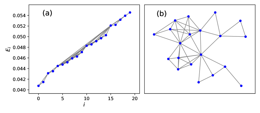
Figure 1: (a) The behavior of a segment $E_{i}$, where the grey lines corresponds to the connected edges under the VG criteria. (b) A topologically equivalent network configuration of (a).

III Degree Distributions

Among various topological characterizations of a complex network, the most important one is the distribution of its vertices’ degrees. A degree of a vertex $\left(i,E_{i}\right)$, denoted by $k_{i}$, is defined as the number of vertices that are connected with $\left(i,E_{i}\right)$ under the VG criteria. By VG’s construction we know that each vertex (except for the starting and ending ones) is at least connected to its two neighbors, i.e. $k_{i}\geq 2$. We are most interested in the probability distribution $P\left(k\right)$ and its mean value $\langle k\rangle$. For a demonstration, we take out one sample from the dataset with $h=1$ and $h=5$, which belong to the thermal and MBL phase respectively, the corresponding $P\left(k\right)$ are drawn in Fig.2(a).

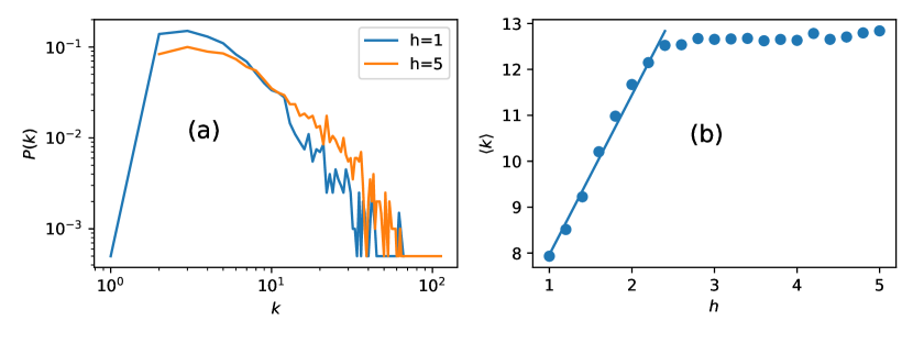
Figure 2: (a) The degree distribution $P(k)$ of a typical spectrum in the thermal ($h=1$) and MBL ($h=5$) phase, the latter has significantly larger $k$. (b) $\langle k\rangle$ as a function of randomness strength $h$.

As we can see, the VG of the MBL phase has significantly larger values of $k$ than that of the thermal phase, which indicates the larger eigenvalue repulsion will results in smaller edge degrees. This hints us the mean value of the edge degree $\langle k\rangle$ may be used to signature the eigenvalue evolution during the thermal-MBL transition. We therefore compute $\langle k\rangle$ among all spectra samples, and plot them as a function of the randomness strength $h$ in Fig.2(b). Interestingly, we find that $\langle k\rangle$ grows linearly with the randomness strength $h$ in the thermal phase, whose formula is fitted to be $\langle k\rangle\simeq 3.48h+4.49$. While $\langle k\rangle$ saturates to a value $\langle k\rangle\simeq 12.8$ at $h\simeq 2.6$, which is close to the thermal-MBL transition point $h_{c}\simeq 3$Regnault16 ; Regnault162 ; Rao21 . This means $\langle k\rangle$ is capable of reflecting the eigenvalue evolution during the phase transition, which is the first non-trivial finding of this work.

To further explore the implication of $\langle k\rangle$ on eigenvalue statistics, recall the normal way to characterize the eigenvalue statistics in random matrix theory is the probability distribution of the level spacings $\left\{s_{i}=E_{i+1}-E_{i}\right\}$, which follows the GOE distribution $P\left(s\right)=\frac{\pi}{2}se^{-\pi s^{2}/4}$ in the thermal phase and the Poisson distribution $P(s)=e^{-s}$ in the MBL phase, both of which are comprised a polynomial term that reflects the level repulsion (or equivalently the system’s symmetry) and an exponential term that reflects the large-$s$ decaying (or the level rigidity). This reminds us the widely-accepted formula for the $P\left(s\right)$ evolution during thermal-MBL transition proposed by Serbyn and MooreSerbyn , i.e.

$$P\left(\beta_{1},\beta_{2},s\right)=C_{1}s^{\beta_{1}}\exp\left(-C_{2}s^{2-\beta_{2}}\right)\text{.}$$ (3)

where  $C_{1},C_{2}$ are normalization parameters determined by $\int P\left(s\right)ds=\int sP\left(s\right)ds=1$. For case deep in the thermal phase, we have $\beta_{1}=1,\beta_{2}=0$ standing for the GOE distribution; and for case deep in the MBL phase, $\beta_{1}=0,\beta_{2}=1$ corresponding to the Poisson ensemble. Ref.[Serbyn, ] shows that the exponential parameters $\beta_{2}$ evolves faster than the polynomial term, i.e. $\beta_{2}$ saturates to $1$ before the transition happens, which is attributed to the Griffiths regime near the transition point. Since we also find the saturation of $\langle k\rangle$ happens earlier than the MBL transition in Fig.2(b), we are led to propose that $\langle k\rangle$ only reflects the exponential term of $P(s)$, while is incapable of detecting the short-range level repulsion term, in other words, it is insensitive to the system’s symmetry.

To verify above idea, we conduct two comparative tests. The first one is the the Gaussian $\beta$ ensemble which generalizes the conventional Wigner classes with $\beta=1,2,4$ to arbitrary positive value of $\beta$, and hence $P\left(\beta,s\right)\sim s^{\beta}e^{-C\left(\beta\right)s^{2}}$. If our conjecture holds, all $\beta$ ensembles should have identical $\langle k\rangle$ in their VGs. The eigenvalue spectra of $\beta$ ensemble can be obtained by diagonalizing the following tridiagonal “parent” matrixBeta

$$M_{\beta}=\frac{1}{\sqrt{2}}\left(\begin{array}[]{ccccc}x_{1}&y_{1}&&&\\ y_{1}&x_{2}&y_{2}&&\\ &\begin{array}[]{ccc}\text{.}&&\\ &\text{.}&\\ &&\text{.}\end{array}&\begin{array}[]{ccc}\text{.}&&\\ &\text{.}&\\ &&\text{.}\end{array}&\begin{array}[]{ccc}\text{.}&&\\ &\text{.}&\\ &&\text{.}\end{array}&\\ &&y_{N-2}&x_{N-1}&y_{N-1}\\ &&&y_{N-1}&x_{N}\end{array}\right)$$ (4)

where the diagonals $x_{i}\,$($i=1,2,...,N$) follow the normal distribution $\mathit{N}\left(0,2\right)$, and $y_{k}$ ($k=1,2,...,N-1$) follows the $\chi$ distribution with parameter $\left(N-k\right)\beta$. When $\beta=1$, it reduces to the standard GOE. Without loss of generality, we select two non-standard values of $\beta=0.4,0.8$, together with the standard GOE ($\beta=1$), and compute the corresponding $\langle k\rangle$ after transforming them into VGs, and the results are given in Table I, as expected, they are quite close.

For the second model, we consider the short-range plasma model (SRPM) that frequently appears in the study of intermediate random matrix ensemblesSRPM , which is widely accepted as the critical distribution at the MBL transition point. SRPM treats the eigenvalues spectrum as an ensemble of one-dimensional particles with only nearest neighboring logarithmic interactions, and it is knownSRPM that the large $s$ behavior of its level spacing follows $P\left(s\right)\sim s^{\beta}e^{-\left(\beta+1\right)s}$ where $\beta$ is the Dyson index controlling the strength of level repulsion. It is well-established that the eigenvalue spectrum of SRPM with index $\beta$ is identical to the spectrum comprised of every $\left(\beta+1\right)$-th eigenvalue from the Poisson ensembleDaisy , which enables us to effectively obtain SRPM’s eigenvalue spectra to do VG analysis. If our conjecture is corrected, the $\langle k\rangle$ of SRPM with different $\beta$ should all be close to the Poisson ensemble. We select $\beta=1,2$ as representative examples, and confirm this conjecture, as shown in Table I.

Model	$\beta=0.4$	$\beta=0.8$	$\beta=1$(GOE)	Poisson	SRPM$\left(\beta=1\right)$	SRPM$\left(\beta=2\right)$
$\langle k\rangle$	8.19	8.14	8.23	14.49	14.55	14.60

Table 1: $\langle k\rangle$ in several random matrix ensembles. The first three are the Gaussian $\beta$ ensembles, whose level spacing distribution decays as $e^{-s^{2}}$; the rest are Poisson/SRPM, with $P(s)$ decays as $e^{-s}$.

To conclude, we have shown that $\langle k\rangle$ is able to reflect the evolution of the exponential term of the level spacing distribution – which is a long-range level correlation, while it is insensitive to the short-range level repulsion parameter, which results in an under-estimation for the thermal-MBL transition point. In fact, similar results have been reported using the SVD method in Ref.[Rao22, ], which together justifies the idea that treats the eigenvalue spectra as time series. To further explore the usefulness of the VG algorithm, we are led to the next section.

IV Clustering and shortest-path-lengths

The next crucial characterization of a VG is the clustering coefficient $c_{i}$ of a vertex, which is defined as

$$c_{i}=\frac{D_{i}}{k_{i}\left(k_{i}-1\right)/2}$$ (5)

where $k_{i}$ is the degree of vertex $i$, and $D_{i}$ is the number of edges between these $k_{i}$ vertices that are connected to $i$. Clearly, the maximum value of $D_{i}$ is $k_{i}\left(k_{i}-1\right)/2$, and so $c_{i}\in[0,1]$. The value of $c_{i}$ measures how close the $i$-th vertex’s connected vertices are clustered together, which explains its name.

We compute the average value of the clustering coefficients $\langle c\rangle$ of the VGs generated from eigenvalue spectra in different randomness strengths. Unlike the degree distribution in previous section, we do not find significant differences in $\langle c\rangle$ between the thermal and MBL phases. Specifically, for VGs from $h=1,2,3,4,5$, we find $\langle c\rangle=0.74,0.72,0.71,0.71,0.71$ respectively.

Above result means the clustering is not a quantity that is sensitive to eigenvalue evolution, but this is not the end of the story. In the context of complex network, a densely clustered network could be a regular network or a “small world” (SW) networkSci1999 ; Nat1998 . The SW network is signatured by the existence of “short cuts” in a network, typical examples include the social network and neural network. To identify an SW network, we need to study the shortest-path-lengths. In a complex network, two disconnected vertices $i$ and $j$ can be connected by several intermediate edges, which is called a path, its length is defined as the number of these internal edges. The path between two vertices are generally not unique, and we are most interested in the shortest one. In an SW network, the mean shortest-path-length $L$ grows logarithmically with the network’s size $N$, that is

$$L\left(N\right)\sim\ln N.$$ (6)

for large $N$.

We therefore calculated the $L\left(N\right)$ for the VGs of the physical eigenvalue spectra, and find that $L(N)$ in the thermal phase has clear $\ln N$ behavior, which maintains even to the transition region; while for MBL phase $L\left(N\right)$ will saturates to a finite value, as demonstrated in Fig.3, where we select $h=1,3,5$ to represent the thermal phase, transition region and MBL phase respectively. Therefore, combined with the large clustering coefficient, we conclude the VGs in thermal and transition region have SW structures.

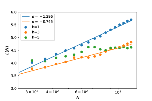
Figure 3: The mean shortest-path-length $L(N$) as a function of $N$, where the x-axis is plotted using a log scale. Clear small-world structure $L(N)\sim ln(N)$ appears in the thermal phase ($h=1$), which maintains even to the transition region ($h=3$).

To this stage, we are able to use the VG characterizations to distinguish the thermal, MBL phases and transition region, as sketched in Table II. This justifies the basic usefulness of the VG algorithm.

	Thermal	Transition	MBL
$\langle k\rangle$	Small	Large	Large
SW	Yes	Yes	No

Table 2: The qualitative criteria to distinguish thermal, MBL phases and transition region using VG’s topological characterizations.

V Cases with incomplete eigenvalue spectra

Despite the ability to distinguish phases, to make this work worthwhile, it’s still questionable about VG’s advantage over traditional approaches. To verify this, we consider the case that the eigenvalue spectra are incomplete with missing levels. The situation of missing levels is common from the experimental aspect, particularly in the area of heavy nuclei, which is exactly the initial playground of random matrix theory back in the 1960s. Analytical treatment for the cases with missing levels can be performed via high-order level spacing distributions, as studied in Ref.[Bohigas, ]. However, since the VG is by construction a topological object, as demonstrated in Fig.1, it is hopeful that the topological characterizations of VGs are robust to spectra with missing levels, at least when the missing probability is not too larger.

To simulate an incomplete spectrum, we set a quantity $p$ that is the probability a level is missing in a spectrum, and so we will end up with a spectrum with mean length $N_{d}*(1-p)$. We then turn the incomplete spectra into VGs, and explore whether the characterizations of the latter are similar to the case with complete spectra.

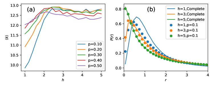
Figure 4: (a) The evolution of $\langle k\rangle$ as a function of randomness strength $h$ in spectra with missing levels, where the probability of missing a level is $p$. The evolution resembles the case with complete spectra in Fig.2(b) up to $p=0.4$. While when $p$ approaches $0.5$, the VG structure breaks down. (b) The normal spacing ratio distribution of the complete spectra and incomplete spectra with $p=0.1$ at the ergodic ($h=1$), MBL ($h=5$) and transition region ($h=3$).

As it turns out, the mean degree $\langle k\rangle$ is robust. In Fig.4(a), we draw the evolution of $\langle k\rangle$ as a function of randomness strength $h$ in cases with level missing probability $p\in[0.1,0.5]$. We see the tendency of $\langle k\rangle$ is similar to the complete spectra case (that is, $\langle k\rangle$ grows with increasing $h$, and saturates before the transition point) even when $p\sim 0.4$, which is a fairly large value. When $p$ grows to $0.5$, the number of missing levels is close to the kept levels, and hence the structure of VG breaks down, and $\langle k\rangle$ becomes fluctuating.

For a heuristic comparison, we also computed the commonly studied spacing ratio distribution $P(r)$, where $\left\{r_{i}=\frac{E_{i+2}-E_{i+1}}{E_{i+1}-E_{i}}\right\}$ in the complete spectra and incomplete spectra with a small $p=0.1$, the results are displayed together in Fig.4(b), where we choose $h=1,5,3$ to represent the thermal, MBL and transition region respectively. As we can see, the deviations between complete and incomplete spectra are larger in the thermal phase than in the MBL phase, which is expected since the eigenvalue correlations in the former are larger, hence the effect of missing levels will be more severe. In fact, we find that $P(r)$ of the incomplete spectra in the thermal phase ($h=1$) is quite close to the transition area ($h=3$), which destroys the possibility to identify phases from $P(r)$. This situation becomes more severe when missing probability grows. These results, together with Fig.4(a), further justifies the advantage of the VG algorithm.

On the other hand, the tests for the mean shortest-path length $L(N)$ do not give conclusive results. This is because the length of incomplete spectrum is not large enough, so the dependence of $L(N)$ on $N$ is ambiguous between polynomial and logarithmic. To improve the result we need to obtain more spectra samples with larger system sizes, which is unaccessible with our current computational resources. Nevertheless, the results for $\langle k\rangle$ in Fig.4 have verified the VG’s applicability in the case with missing levels.

VI Conclusion and Discussion

With the central idea that treats the eigenvalue spectra as multi-variant time series, in this work we employed the visibility graph (VG) algorithm to make a complex network analysis on the eigenvalues of random spin systems. The main findings are as follows.

First of all, we find the degree distribution of the VGs generated from eigenvalue spectra can faithfully reflects the evolution of eigenvalue statistics, specifically, spectra with larger correlation in the thermal phase have significantly smaller degrees than the MBL phase with uncorrelated spectra. We also verified the mean degree $\langle k\rangle$ is closely related to the exponential term in the level spacing distribution, while is insensitive to the short-range level repulsion, or the system’s symmetry. Second, we find that the spectra in the thermal phase have a small-world structure, which maintain even to the transition region. Thus, the degree distribution and SW structure can be utilized together to distinguish the thermal, MBL and transition regions. Last but not least, we show the VG algorithm is applicable in cases with incomplete spectra, which stems from VG’s topological construction and reveals the advantage of the complex network methodologies.

It is worth noting that the VG employed in this work is one of the simplest complex network configurations, while it is already capable of providing non-trivial physical information, which justifies the validity of employing complex networks to study the disordered quantum systems. Present paper serves as a preliminary work in this direction that is by no means complete, there is certainly many future directions to explore. To name just a few here. First of all, there are many other network characteristics that do not appear in this work, such as the adjacent matrix and assortive mixing, their relation to the eigenvalue correlations deserves to be explored. Second, the VG employed in this work is insensitive to the system’s symmetry, which may attribute to its simple construction, its tempting to bring some sophistication to VGs, for instance by adding weights and directions to the edges. Third, complex networks naturally captures the long-range level correlations in a spectrum, hence it’s hopefully to study subtle physical quantities like Thouless energy and Grifiths regime, during which the unfolding procedure can be avoided. This necessarily requires larger datasets, and will be studied in a future work.

VII Acknowledgements

This work is supported by the Zhejiang Provincial Natural Science Foundation of China under Grant No.LY23A050003.

Data Availibility Statement: The data that support the figures within this paper are available from the corresponding author upon reasonable request.

References

- (1) J. A. Kjall, J. H. Bardarson, and F. Pollmann, Phys. Rev. Lett. 113, 107204 (2014).
- (2) Z. C. Yang, C. Chamon, A. Hamma, and E. R. Mucciolo, Phys. Rev. Lett. 115, 267206 (2015).
- (3) M. Serbyn, A. A. Michailidis, M. A. Abanin, and Z. Papic, Phys. Rev. Lett. 117, 160601 (2016).
- (4) M. Serbyn, Z. Papić, and D. A. Abanin, Phys. Rev. X 5, 041047 (2015).
- (5) H. Kim and D. A. Huse, Phys. Rev. Lett. 111, 127205 (2013).
- (6) J. H. Bardarson, F. Pollman, and J. E. Moore, Phys. Rev. Lett. 109, 017202 (2012).
- (7) M. Serbyn, Z. Papić, and D. A. Abanin, Phys. Rev. B 90, 174302 (2014).
- (8) C. L. Bertrand and A. M. García-García, Phys. Rev. B 94, 144201 (2016).
- (9) M. L. Mehta, Random Matrix Theory, Springer, New York (1990).
- (10) F. Haake, Quantum Signatures of Chaos, (Springer 2001).
- (11) V. Oganesyan and D. A. Huse, Phys. Rev. B 75, 155111 (2007).
- (12) Y. Avishai, J. Richert, and R. Berkovits, Phys. Rev. B 66, 052416 (2002).
- (13) N. Regnault and R. Nandkishore, Phys. Rev. B 93, 104203 (2016).
- (14) S. D. Geraedts, R. Nandkishore, and N. Regnault, Phys. Rev. B 93, 174202 (2016).
- (15) V. Oganesyan, A. Pal, D. A. Huse, Phys. Rev. B 80, 115104 (2009).
- (16) A. Pal, D. A. Huse, Phys. Rev. B 82, 174411 (2010).
- (17) S. Iyer, V. Oganesyan, G. Refael, D. A. Huse, Phys. Rev. B 87, 134202 (2013).
- (18) D. J. Luitz, N. Laflorencie, and F. Alet, Phys. Rev. B 91, 081103(R) (2015).
- (19) M. Serbyn and J. E. Moore, Phys. Rev. B 93, 041424(R) (2016).
- (20) P. Sierant and J. Zakrzewski, Phys. Rev. B 99, 104205 (2019).
- (21) P. Sierant and J. Zakrzewski, Phys. Rev. B 101, 104201 (2020).
- (22) P. Sierant, D. Delande, and J. Zakrzewski, Phys. Rev. Lett. 124, 186601 (2020).
- (23) A. M. García-García, Phys. Rev. E 73, 026213 (2006).
- (24) A. Relãno, J. M. G. Gómez, R. A. Molina, J. Retamosa, and E. Faleiro, Phys. Rev. Lett. 89, 244102 (2002).
- (25) E. Faleiro, J. M. G. Gómez, R. A. Molina, L. Muñoz, A. Relaño, and J. Retamosa, Phys. Rev. Lett. 93, 244101 (2004).
- (26) A. Relaño, L. Muñoz, J. Retamosa, E. Faleiro, and R. A. Molina, Phys. Rev. E 77, 031103 (2008).
- (27) R. Riser, V. Al. Osipov, and E. Kanzieper, Phys. Rev. Lett. 118, 204101 (2017).
- (28) R. Fossion, G. Torres-Vargas, and J. C. López-Vieyra, Phys. Rev. E, 88, 060902(R) (2013).
- (29) J. M. G. Gomez, R. A. Molina, A. Relaño, and J. Retamosa, Phys. Rev. E 66, 036209 (2002).
- (30) A. D. Jackson, C. Mejia-Monasterio, T. Rupp, M. Saltzer, and T. Wilke, Nuclear Physics A 687, 405-434 (2001).
- (31) R. Fossion, G. Torres-Vargas, V. Velázquez and J. C. López-Vieyra, Journal of Physics: Conference Series 578, 012013 (2015).
- (32) G. Torres-Vargas and R. Fossion, Physica A 545, 123128 (2020).
- (33) G. Torres-Vargas, R. Fossion and J. A. Méndez-Bermúdez, Physica A 545, 123298 (2020).
- (34) G. Torres-Vargas, R. Fossion, C. Tapia-Ignacio, and J. C. López-Vieyra, Phys. Rev. E, 96, 012110 (2017).
- (35) G. Torres-Vargas, J. A. Méndez-Bermúdez, J. C. López-Vieyra, and R. Fossion, Phys. Rev. E, 98, 022110 (2018).
- (36) V. E. Kravtsov, I. M. Khaymovich, E. Cuevas, and M. Amini, New J. Phys. 17, 122002 (2015).
- (37) R. Berkovits, Phys. Rev. B 102, 165140 (2020).
- (38) R. Berkovits, Phys. Rev. B 104, 054207 (2021).
- (39) R. Berkovits, Phys. Rev. B 105, 104203 (2022).
- (40) R. Berkovits, Phys. Rev. B 107, 035141 (2023).
- (41) R. Berkovits, EPL 142, 56001 (2023).
- (42) W.-J. Rao, Phys. Rev. B 105, 054207 (2022).
- (43) W.-B. Ni and W.-J. Rao, Eur. Phys. J. Plus 137, 534 (2022).
- (44) W. F. Xu and W. J. Rao, Sci. Rep. 13, 634 (2023).
- (45) Y. Zou, R. V. Donner, N. Marwan, J. F. Donges and J. Kurths, Phys. Rep., 787, 1-97 (2019).
- (46) J. Zhang and M. Small, Phys. Rev. Lett., 96, 238701 (2006).
- (47) J. Zhang, J.-F. Sun, X.-D. Luo, K. Zhang, T. Nakamura, and M. Small, Physica D 237, 2856 (2008).
- (48) Y. Yang, H.-J. Yang, Complex network-based time series analysis, Physica A 387, 1381 (2008).
- (49) R. V. Donner, Y. Zou, J. F. Donges, N. Marwan, and J. Kurths, New J. Phys. 12, 033025 (2010).
- (50) P.-F. Dai, X. Xiong, and W.-X. Zhou, Physica A 531, 121748 (2019).
- (51) L. Lacasa, B. Luque, F. Ballesteros, J. Luque, and J. C. Nuño, Proc. Natl. Acad. Sci. U.S.A. 105(13), 4972 (2008).
- (52) I. V. Bezsudnov and A. A. Snarskii, Physica A 414, 53 (2014).
- (53) D. J. Watts and S. H. Strogatz, Nature 393, 440 (1998).
- (54) S. Jalan and J. N. Bandyopadhyay, Phys. Rev. E 76, 046107 (2007).
- (55) J. N. Bandyopadhyay and S. Jalan, Phys. Rev. E 76, 026109 (2007).
- (56) W.-J. Rao, J. Phys. A: Math. Theor. 54, 105001 (2021).
- (57) B. Luque, L. Lacasa, F. Ballesteros and J. Luque, Phys. Rev. E 80, 046103 (2009).
- (58) I. Dumitriu and A. Edelman, J. Math. Phys. (N.Y.) 43, 5830 (2002).
- (59) E. B. Bogomolny, U. Gerland and C. Schmit, Eur. Phys. J. B 19, 121 (2001).
- (60) H. Hernández-Saldaña, J. Flores, and T. H. Seligman, Phys. Rev. E 60, 449 (1999).
- (61) A. Barabasi and R. Albert, Science, 286, 509 (1999).
- (62) O. Bohigas and M. P. Pato, Phys. Lett. B 595, 171 (2004).