Lewis’s Signaling Game as beta-VAE
For Natural Word Lengths and Segments

Abstract

As a sub-discipline of evolutionary and computational linguistics, emergent communication (EC) studies communication protocols, called emergent languages, arising in simulations where agents communicate. A key goal of EC is to give rise to languages that share statistical properties with natural languages. In this paper, we reinterpret Lewis’s signaling game, a frequently used setting in EC, as beta-VAE and reformulate its objective function as ELBO. Consequently, we clarify the existence of prior distributions of emergent languages and show that the choice of the priors can influence their statistical properties. Specifically, we address the properties of word lengths and segmentation, known as Zipf’s law of abbreviation (ZLA) and Harris’s articulation scheme (HAS), respectively. It has been reported that the emergent languages do not follow them when using the conventional objective. We experimentally demonstrate that by selecting an appropriate prior distribution, more natural segments emerge, while suggesting that the conventional one prevents the languages from following ZLA and HAS.

Keywords Emergent Communication, Emergent Language, Probabilistic Generative Model, Variational Autoencoder, beta-VAE, Zipf’s law of abbreviation, Harris’s articulation scheme

1 Introduction

Understanding how language and communication emerge is one of the ultimate goals in evolutionary linguistics and computational linguistics. Emergent communication (EC, Lazaridou & Baroni, 2020; Galke et al., 2022; Brandizzi, 2023) attempts to simulate the emergence of language using techniques such as deep learning and reinforcement learning. A key challenge in EC is to elucidate how emergent communication protocols, or emergent languages, reproduce statistical properties similar to natural languages, such as compositionality (Kottur et al., 2017; Chaabouni et al., 2020; Ren et al., 2020), word length distribution (Chaabouni et al., 2019; Rita et al., 2020), and word segmentation (Resnick et al., 2020; Ueda et al., 2023). In this paper, we reformulate Lewis’s signaling game (Lewis, 1969; Skyrms, 2010), a popular setting in EC, as beta-VAE (Kingma & Welling, 2014; Higgins et al., 2017) for the emergence of more natural word lengths and segments.

Lewis’s signaling game and its objective: Lewis’s signaling game is frequently adopted in EC (e.g., Chaabouni et al., 2019; Rita et al., 2022b). It is a simple communication game involving a sender $S_{\bm{\phi}}$ and receiver $R_{\bm{\theta}}$, with only unidirectional communication allowed from $S_{\bm{\phi}}$ to $R_{\bm{\theta}}$. In each play, $S_{\bm{\phi}}$ obtains an object $x$ and converts it into a message $m$. Then, $R_{\bm{\theta}}$ interprets $m$ to guess the original object $x$. The game is successful upon a correct guess. $S_{\bm{\phi}}$ and $R_{\bm{\theta}}$ are typically represented as neural networks such as RNNs (Hochreiter & Schmidhuber, 1997; Cho et al., 2014) and optimized for a certain objective $\mathcal{J}_{\textrm{conv}}$, which is in most cases defined as the maximization of the log-likelihood of the receiver’s guess (or equivalently minimization of cross-entropy loss).

ELBO as objective: In contrast, we propose to regard the signaling game as (beta-)VAE (Kingma & Welling, 2014; Higgins et al., 2017) and utilize ELBO (with a KL-weighing parameter $\beta$) as the game objective. We reinterpret the game as representation learning in a generative model, regarding $x$ as an observed variable, $m$ as latent variable, $S_{\bm{\phi}}$ as encoder, $R_{\bm{\theta}}$ as decoder, and an additionally introduced “language model” $P^{\textrm{prior}}_{\bm{\theta}}$ as prior latent distribution. Several reasons support our reformulation. First, the conventional objective $\mathcal{J}_{\textrm{conv}}$ actually resembles ELBO in some respects. We illustrate their similarity in Figure 1 and Table 1. $\mathcal{J}_{\textrm{conv}}$ has an implicit prior message distribution, while ELBO contains explicit one. Also, $\mathcal{J}_{\textrm{conv}}$ is often adjusted with an entropy regularizer while ELBO contains an entropy maximizer. Although they are not mathematically equal, their motivations coincide in that they keep the sender’s entropy high to encourage exploration (Levine, 2018). Second, the choice of a prior message distribution can affect the statistical properties of emergent languages. Specifically, this paper addresses Zipf’s law of abbreviation (ZLA, Zipf, 1935, 1949) and Harris’s articulation scheme (HAS, Harris, 1955; Tanaka-Ishii, 2021). It has been reported that they are not reproduced in emergent languages, as long as the conventional objective $\mathcal{J}_{\textrm{conv}}$ is used (Chaabouni et al., 2019; Ueda et al., 2023). We suggest that such an artifact is caused by unnatural prior distributions and that it has been obscure due to their implicitness. Moreover, our ELBO-based formulation can be justified from the computational psycholinguistic point of view, namely surprisal theory (Hale, 2001; Levy, 2008; Smith & Levy, 2013). The prior term can be seen as the surprisal, or cognitive processing cost, of sentences (messages). In that sense, ELBO naturally models the trade-off between the informativeness and processability of sentences.

Related work and contribution: The idea per se of viewing communication as representation learning is also seen in previous work. For instance, the linguistic concept compositionality is often regarded as disentanglement (Andreas, 2019; Chaabouni et al., 2020; Resnick et al., 2020). Also, Tucker et al. (2022) formulated a VQ-VIB game based on Variational Information Bottleneck (VIB, Alemi et al., 2017), which is known as a generalization of beta-VAE. Moreover, Taniguchi et al. (2022) defined a Metropolis-Hastings (MH) naming game in which communication was formulated as representation learning on a generative model and emerged through MCMC. However, to the best of our knowledge, no previous work has addressed in an integrated way (1) the similarities between the game and (beta-)VAE from the generative viewpoint, (2) the potential impact of prior distribution on the properties of emergent languages, and (3) a computational psycholinguistic reinterpretation of emergent communication. They are the main contribution of this paper.

Revisiting Variable-Length Setting: Another important point is that, since Chaabouni et al. (2019), most EC work on signaling games has adopted either the one-character-as-one-message or fixed-length message setting, avoiding the variable-length setting, though the variable-length is more natural. We revisit the variable-length setting towards the better simulation of language emergence.

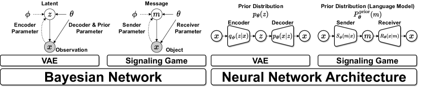
Figure 1: Illustration of similarity between signaling games and (beta-)VAE.

Table 1: A list of objective functions in this paper. It is useful to grasp their similarity.

objective	definition	prior (implicit/explicit)	entropy-related term
$\mathcal{J}_{\textrm{conv}}(\bm{\phi},\bm{\theta})$	Eq. 2 (Section 2)	$P^{\textrm{prior}}_{\textrm{unif}}(M)$ (implicit)	entropy regularizer
$\mathcal{J}_{\textrm{conv}}(\bm{\phi},\bm{\theta};\alpha)$	Eq. 4 (Section 2)	$P^{\textrm{prior}}_{\alpha}(M)$ (implicit)	entropy regularizer
$\mathcal{J}_{\textrm{elbo}}(\bm{\phi},\bm{\theta};\alpha)$	Eq. 12 (Section 3)	$P^{\textrm{prior}}_{\alpha}(M)$ (explicit)	entropy maximizer
$\mathcal{J}_{\textrm{ours}}(\bm{\phi},\bm{\theta};\beta)$	Eq. 7 (Section 3)	$P^{\textrm{prior}}_{\bm{\theta}}(M)$ (explicit)	entropy maximizer

2 Background

2.1 Language Emergence via Lewis’s Signaling Game

To simulate language emergence, defining an environment surrounding agents is necessary. One of the most standard settings in EC is Lewis’s signaling game (Lewis, 1969; Skyrms, 2010; Rita et al., 2022b), though there are several variations in the environment definition (Foerster et al., 2016; Lowe et al., 2017; Mordatch & Abbeel, 2018; Jaques et al., 2019, inter alia). The game involves two agents, sender $S$ and receiver $R$. In a single play, the sender $S$ observes an object $x$ and generates a message $m$. The receiver $R$ obtains the message $m$ and guesses the object $x$. The game is successful if the guess is correct. More formally, let $\mathcal{X}$ be an object space, $\mathcal{M}$ be a message space, $P_{\textrm{obj}}(X)$ be a probability of objects, a conditional probability $S_{\bm{\phi}}(M|X)$ be a sender, and a conditional probability $R_{\bm{\theta}}(X|M)$ be a receiver. $S_{\bm{\phi}}$ and $R_{\bm{\theta}}$ are often represented as RNNs by $\bm{\phi}$ and $\bm{\theta}$ respectively and optimized towards successful communication. During training, the sender probabilistically observes an object $x\sim P_{\textrm{obj}}(\cdot)$, generates a message $m\sim S_{\bm{\phi}}(\cdot|x)$, and the receiver guesses via $\log R_{\bm{\theta}}(x|m)$. During validation, the sender observes $x$ one by one and greedily generates $m$.

Object Space: Objects $x$ can be defined in various ways, from abstract to realistic data. In this paper, an object $x$ is assumed to be an attribute-value (att-val) object (Kottur et al., 2017; Chaabouni et al., 2020) which is a $n_{\textrm{att}}$-tuple of integers $(v_{1},\ldots,v_{n_{\textrm{att}}})\in\mathcal{X}$, where $v_{i}\in\{1,\ldots,n_{\textrm{val}}\}$ for each $i$. $n_{\textrm{att}}$ is called the number of attributes and $n_{\textrm{val}}$ is called the number of values.

Message Space: In most cases, the message space $\mathcal{M}$ is defined as a set of sequences of a (maximum) length $L_{\textrm{max}}$ over a finite alphabet $\mathcal{A}$. The message length, denoted by $|m|$, can be either fixed (Chaabouni et al., 2020) or variable (Chaabouni et al., 2019). This paper adopts the latter setting:

$$\mathcal{M}:=\{m_{1}\cdots m_{k}\in\mathcal{A}^{*}\mid m_{i}\neq\texttt{eos}~{}(1\leq i\leq k-1),m_{k}=\texttt{eos},1\leq k\leq L_{\textrm{max}}\},$$ (1)

where $\texttt{eos}\in\mathcal{A}$ is the end-of-sequences marker. We assume $\mathcal{A}$ contains at least 2 symbols other than eos (thus $\log(|\mathcal{A}|-1)>0$).

Game Objective: The game objective is often defined as (Chaabouni et al., 2019; Rita et al., 2022b):

$$\mathcal{J}_{\textrm{conv}}(\bm{\phi},\bm{\theta}):=\mathbb{E}_{x\sim P_{\textrm{obj}}(\cdot),m\sim S_{\bm{\phi}}(\cdot|x)}\left[\log R_{\bm{\theta}}(x\mid m)\right].$$ (2)

For clarity, we refer to $\mathcal{J}_{\textrm{conv}}$ as the conventional objective, in contrast to our objective $\mathcal{J}_{\textrm{ours}}$ defined later. The parameters $\bm{\phi},\bm{\theta}$ are updated via the stochastic gradient method. In practice, an entropy regularizer (Williams & Peng, 1991; Mnih et al., 2016) is added to $\nabla_{\bm{\phi},\bm{\theta}}\mathcal{J}_{\textrm{conv}}(\bm{\phi},\bm{\theta})$:

$$\nabla_{\bm{\phi},\bm{\theta}}^{\textrm{ent-reg}}:=\frac{\lambda^{\textrm{entreg}}}{|m|}\sum\nolimits_{t=1}^{|m|}\nabla_{\bm{\phi},\bm{\theta}}\mathcal{H}(S_{\bm{\phi}}(A_{t}\mid x,m_{1:t-1})),$$ (3)

where $\lambda^{\textrm{entreg}}$ is a hyperparameter adjusting the weight. It encourages the sender agent to explore the message space during training by keeping its policy entropy high. A message-length penalty $-\alpha|m|$ is sometimes added to the objective to prevent messages from becoming unnaturally long:

$$\mathcal{J}_{\textrm{conv}}(\bm{\phi},\bm{\theta};\alpha):=\mathbb{E}_{x\sim P_{\textrm{obj}}(\cdot),m\sim S_{\bm{\phi}}(\cdot|x)}\left[\log R_{\bm{\theta}}(x\mid m)-\alpha|m|\right].$$ (4)

Chaabouni et al. (2019) and Rita et al. (2020) pointed out that the message-length penalty is necessary to give rise to Zipf’s law of abbreviation (ZLA) in emergent languages.

2.2 On the Statistical Properties of Languages

It is a key challenge in EC to fill the gap between emergent and natural languages. Though it is not straightforward to evaluate the emergent languages that are uninterpretable for human evaluators, their natural language likeness has been assessed indirectly by focusing on their statistical properties (e.g., Chaabouni et al., 2019; Kharitonov et al., 2020). We briefly introduce previous EC studies on compositionality, Zipf’s law of abbreviation, and Harris’s articulation scheme.

Compositionality: In EC, compositionality is frequently studied (Kottur et al., 2017; Chaabouni et al., 2020; Li & Bowling, 2019; Andreas, 2019; Ren et al., 2020). The standard compositionality measure is Topographic Similarity (TopSim, Brighton & Kirby, 2006; Lazaridou et al., 2018). Let $d_{\mathcal{X}}$ be a distance function in an object space and $d_{\mathcal{M}}$ in a message space. TopSim is defined as the Spearman correlation between $d_{\mathcal{X}}(x^{(1)},x^{(2)})$ and $d_{\mathcal{M}}(m^{(1)},m^{(2)})$ for all combinations $x^{(1)},x^{(2)}\in\mathcal{X}$ (without repetition). Here, each $m^{(i)}$ is the greedy sample from $S_{\bm{\phi}}(M|x^{(i)})$. $d_{\mathcal{X}}$ and $d_{\mathcal{M}}$ are usually defined as Hamming and Levenshtein distance, respectively.

Word Lengths: Zipf’s law of abbreviation (ZLA, Zipf, 1935, 1949) refers to the statistical property of natural language where frequently used words tend to be shorter. Chaabouni et al. (2019) reported that emergent languages do not follow ZLA by the conventional objective $\mathcal{J}_{\textrm{conv}}(\bm{\phi},\bm{\theta})$. They defined $P_{\textrm{obj}}(X)$ as a power-law distribution. According to ZLA, it was expected that $|m^{(1)}|<|m^{(2)}|$ overall for $x^{(1)},x^{(2)}$ such that $P_{\textrm{obj}}(x^{(1)})>P_{\textrm{obj}}(x^{(2)})$. Their experiment, however, showed the opposite tendency $|m^{(1)}|>|m^{(2)}|$. They also reported that the emergent languages do follow ZLA when the message-length penalty (Eq. 4) is additionally introduced. Previous work has ascribed such anti-efficiency to the lack of desirable inductive biases, such as the sender’s laziness (Chaabouni et al., 2019) and receiver’s impatience (Rita et al., 2020), and memory constraints (Ueda & Washio, 2021).

Word Segments: Harris’s articulation scheme (HAS, Harris, 1955; Tanaka-Ishii, 2021) is a statistical property of word segmentation in natural languages. According to HAS, the boundaries of word segments in a character sequence can be predicted to some extent from the statistical behavior of character $n$-grams. This scheme is based on the discovery of Harris (1955) that there tend to be word boundaries at points where the number of possible successive characters after given contexts increases in English corpora. HAS reformulates it based on information theory (Cover & Thomas, 2006). Formally, let $\textrm{BE}(s)$ be the branching entropy of character sequences $s\in\mathcal{A}^{*}$:

$$\textrm{BE}(s) {:=}\mathcal{H}(A_{n+1}|A_{1:n}{=}s){=}{-}\sum\nolimits_{a\in\mathcal{A}}P(A_{n+1}{=}a|A_{1:n}{=}s)\log_{2}P(A_{n+1}{=}a|A_{1:n}{=}s),$$ (5)

where $n$ is the length of $s$ and $P(A_{n+1}=a|A_{1:n}=s)$ is defined as a simple $n$-gram model. $\textrm{BE}(s)$ is known to decrease monotonically on average, while its increase can be of special interest. HAS states that there tend to be word boundaries at BE’s increasing points. HAS can be utilized as an unsupervised word segmentation algorithm (Tanaka-Ishii, 2005; Tanaka-Ishii & Ishii, 2007) whose pseudo-code is shown in Appendix A. However, whether obtained segments from emergent languages are meaningful is not obvious. For instance, no one would believe that segments obtained from a monkey typing sequence represent meaningful words; emergent languages face a similar issue as they are not human languages. We do not even have a direct method to evaluate the meaningfulness since there is no ground-truth segmentation data in emergent languages. To alleviate it, Ueda et al. (2023) proposed the following criteria to indirectly verify their meaningfulness:

1. The number of boundaries per message (denoted by $n_{\textrm{bou}}$) should increase if $n_{\textrm{att}}$ increases.

2. The number of distinct segments in a language (denoted by $n_{\textrm{seg}}$) should increase if $n_{\textrm{val}}$ increases.

3. $\textrm{W-TopSim}>\textrm{C-TopSim}$ should hold, or $\Delta_{\textrm{w},\textrm{c}}:=\textrm{W-TopSim}-\textrm{C-TopSim}>0$ should hold.

These are rephrased to some extent. C-TopSim is the normal TopSim that regards characters $a\in\mathcal{A}$ as symbol units, whereas W-TopSim regards segments (chunked characters) as symbol units. The choice of symbol unit may affect Levenshtein distance. In the att-val setting, meaningful segments are expected to represent attributes and values in a disentangled way, motivating C1 and C2. On the other hand, C3 is based on the concept called double articulation by Martinet (1960), who pointed out that, in natural language, characters within a word are hardly related to the corresponding meaning unit whereas the word is related. For instance, characters a, e, l, p are irrelevant to a rounded, red, sweet, and tangy fruit, but word apple is relevant to it. Thus, the word-level compositionality is expected to be higher than the character-level one, motivating C3. With the conventional objective, however, emergent languages did not satisfy any of them, and the potential causes for this have not been addressed well in Ueda et al. (2023).

3 Redefine Objective as ELBO from the Generative Perspective

The main proposal of this paper is to redefine the objective of signaling games as (beta-)VAE’s (Kingma & Welling, 2014; Higgins et al., 2017), i.e., the evidence lower bound (ELBO) with an additional KL weighting hyperparameter $\beta$. Though somewhat abrupt, let us think of a receiver agent $R_{\bm{\theta}}$ as a generative model, or a joint distribution over objects $X$ and messages $M$:

$$R_{\bm{\theta}}^{\textrm{joint}}(X,M):=R_{\bm{\theta}}(X\mid M)P^{\textrm{prior}}_{\bm{\theta}}(M).$$ (6)

Intuitively, the receiver consists not only of the conventional reconstruction term $R_{\bm{\theta}}(X|M)$ but also of a “language model” $P^{\textrm{prior}}_{\bm{\theta}}(M)$. The optimal sender would be the true posterior $S_{\bm{\theta}}^{*}(M|X)=R_{\bm{\theta}}(X|M)P^{\textrm{prior}}_{\bm{\theta}}(M)/P_{\textrm{obj}}(X)$ by Bayes’ theorem. Let us assume, however, that the sender can only approximate it via a variational posterior $S_{\bm{\phi}}(M|X)$. The sender cannot access the true posterior because it is intractable and the sender cannot directly peer into the receiver’s “brain” $\bm{\theta}$. Now one notices the similarity between the signaling game and (beta-)VAE. Their similarity is illustrated in Figure 1 and Table 1. beta-VAE consists of an encoder, decoder, and prior latent distribution. Here, we regard $M$ as latent, $S_{\bm{\phi}}(M|X)$ as encoder, $R_{\bm{\theta}}(X|M)$ as receiver, and $P^{\textrm{prior}}_{\bm{\theta}}(M)$ as prior distribution. Our objective is now defined as follows:

$$\mathcal{J}_{\textrm{ours}}(\bm{\phi},\bm{\theta};\beta) :=\mathbb{E}_{x\sim P_{\textrm{obj}}(\cdot)}[\mathbb{E}_{m\sim S_{\bm{\phi}}(\cdot|x)}[\log R_{\bm{\theta}}(x\mid m)]-\beta D_{\mathrm{KL}}(S_{\bm{\phi}}(M\mid x)|\!|P^{\textrm{prior}}_{\bm{\theta}}(M))],$$ (7)

where $D_{\mathrm{KL}}$ denotes the KL divergence and $\beta\geq 0$ is a hyperparameter that weights the KL term. Although Eq. 7 equals to the precise ELBO only if $\beta=1$, $\beta$ is often set $<1$ initially and (optionally) annealed to $1$ to prevent posterior collapse (Bowman et al., 2016; Alemi et al., 2018; Fu et al., 2019; Klushyn et al., 2019). In what follows, we discuss reasons supporting our redefinition.

3.1 Conventional Objective Has An Implicit Prior Distribution

We show that the conventional signaling game has implicit prior distributions $P^{\textrm{prior}}_{\textrm{unif}}(M)$ or $P^{\textrm{prior}}_{\alpha}(M)$. First, let $P^{\textrm{prior}}_{\textrm{unif}}(M)$ be a uniform message distribution and $P_{\bm{\theta},\textrm{unif}}^{\textrm{joint}}(X,M)$ be as follows:

$$P^{\textrm{prior}}_{\textrm{unif}}(m)\propto\textrm{const},\quad P_{\bm{\theta},\textrm{unif}}^{\textrm{joint}}(x,m):=R_{\bm{\theta}}(x\mid m)P^{\textrm{prior}}_{\textrm{unif}}(m).$$ (8)

Then, the following holds (see Section B.1 for its proof):

$$\nabla_{\bm{\phi},\bm{\theta}}\mathcal{J}_{\textrm{conv}}(\bm{\phi},\bm{\theta})=\nabla_{\bm{\phi},\bm{\theta}}\mathbb{E}_{x\sim P_{\textrm{obj}}(\cdot),m\sim S_{\bm{\phi}}(\cdot|x)}\bigl{[}\log P_{\bm{\theta},\textrm{unif}}^{\textrm{joint}}(x,m)\bigr{]},$$ (9)

i.e., maximizing $\mathcal{J}_{\textrm{conv}}(\bm{\phi},\bm{\theta})$ via the gradient method is the same as maximizing the expectation of $\log P_{\bm{\theta},\textrm{unif}}^{\textrm{joint}}(x,m)$. Next, the length-penalizing objective $\mathcal{J}_{\textrm{conv}}(\bm{\phi},\bm{\theta};\alpha)$ also has a prior distribution. Let $P^{\textrm{prior}}_{\alpha}(M)$ and $P_{\bm{\theta},\alpha}^{\textrm{joint}}(X,M)$ be as follows:

$$P^{\textrm{prior}}_{\alpha}(m)\propto\exp(-\alpha|m|),\quad P_{\bm{\theta},\alpha}^{\textrm{joint}}(x,m):=R_{\bm{\theta}}(x\mid m)P^{\textrm{prior}}_{\alpha}(m).$$ (10)

Then, the following holds (see Section B.1 for its proof):

$$\nabla_{\bm{\phi},\bm{\theta}}\mathcal{J}_{\textrm{conv}}(\bm{\phi},\bm{\theta};\alpha)=\nabla_{\bm{\phi},\bm{\theta}}\mathbb{E}_{x\sim P_{\textrm{obj}}(\cdot),m\sim S_{\bm{\phi}}(\cdot|x)}[\log P_{\bm{\theta},\alpha}^{\textrm{joint}}(x,m)],$$ (11)

i.e., maximizing $\mathcal{J}_{\textrm{conv}}(\bm{\phi},\bm{\theta};\alpha)$ is the same as maximizing the expectation of $\log P_{\bm{\theta},\alpha}^{\textrm{joint}}(x,m)$. Note that Eq. 8 is a special case of Eq. 10; $P^{\textrm{prior}}_{\textrm{unif}}(m){=}P^{\textrm{prior}}_{\alpha}(m),~{}P_{\bm{\theta},\textrm{unif}}^{\textrm{joint}}(x,m){=}P_{\bm{\theta},\alpha}^{\textrm{joint}}(x,m)$ if $\alpha=0$.

3.2 Conventional Objective Is a Heuristic Variant of (beta-)VAE

The conventional objective may be similar to variational inference on a generative model, as it turned out to have implicit prior distributions. Indeed, it is similar to (beta-)VAE. As $\mathcal{J}_{\textrm{conv}}(\bm{\phi},\bm{\theta};\alpha)$ has the implicit prior $P^{\textrm{prior}}_{\alpha}(M)$, one notices the similarity between the signaling game and VAE, regarding $M$ as latent, $S_{\bm{\phi}}(M|X)$ as encoder, $R_{\bm{\theta}}(X|M)$ as decoder. Here, the corresponding ELBO $\mathcal{J}_{\textrm{elbo}}(\bm{\phi},\bm{\theta};\alpha)$ can be written as follows:

$$\mathcal{J}_{\textrm{elbo}}(\bm{\phi},\bm{\theta};\alpha):=\mathbb{E}_{x\sim P_{\textrm{obj}}(\cdot)}[\mathbb{E}_{m\sim S_{\bm{\phi}}(\cdot\mid x)}[\log R_{\bm{\theta}}(x\mid m)]-D_{\mathrm{KL}}(S_{\bm{\phi}}(M|x)||P^{\textrm{prior}}_{\alpha}(M))].$$ (12)

Then, the following holds (see Section B.3 for its proof):

$$\nabla_{\bm{\phi},\bm{\theta}}\mathcal{J}_{\textrm{elbo}}(\bm{\phi},\bm{\theta};\alpha)=\nabla_{\bm{\phi},\bm{\theta}}\mathcal{J}_{\textrm{conv}}(\bm{\phi},\bm{\theta};\alpha)+\underbrace{\nabla_{\bm{\phi},\bm{\theta}}\mathbb{E}_{x\sim P_{\textrm{obj}}(\cdot)}[\mathcal{H}(S_{\bm{\phi}}(M\mid x))]}_{\text{resembles $\nabla_{\bm{\phi},\bm{\theta}}^{\textrm{ent-reg}}$ (\lx@cref{creftype~refnum}{eq: entropy regularizer})}},$$ (13)

i.e., maximizing $\mathcal{J}_{\textrm{elbo}}(\bm{\phi},\bm{\theta};\alpha)$ is the same as maximizing $\mathcal{J}_{\textrm{conv}}(\bm{\phi},\bm{\theta};\alpha)$ plus an entropy maximizer. Recall that previous work typically adopts an entropy regularizer (Eq. 3). Though they are not mathematically equal, they are similar enough in that they keep the sender’s entropy high to encourage exploration (Levine, 2018). Thus, the conventional game is a heuristic variant of VAE. Or rather, it is similar to beta-VAE because $\lambda^{\textrm{entreg}}$ adjusts the entropy regularizer in practice, which roughly corresponds to that $\beta$ adjusts the KL term weight.

3.3 Implicit Prior Distribution and Inefficiency of Emergent Language

We have thus far seen that the conventional objective has an implicit prior distribution and is a heuristic variant of beta-VAE. Now we need to elaborate on why one should be aware of them. To this end, in this subsection, we suggest that the inefficiency of emergent languages is due to unnatural prior distributions. Chaabouni et al. (2019) reported that the objective $\mathcal{J}_{\textrm{conv}}(\bm{\phi},\bm{\theta})$ did not result in emergent languages that follow ZLA, while the length-penalizing one $\mathcal{J}_{\textrm{conv}}(\bm{\phi},\bm{\theta};\alpha)$ did. Recalling that $\mathcal{J}_{\textrm{conv}}(\bm{\phi},\bm{\theta})$ has the implicit prior distribution $P^{\textrm{prior}}_{\textrm{unif}}(M)$ and $\mathcal{J}_{\textrm{conv}}(\bm{\phi},\bm{\theta};\alpha)$ has $P^{\textrm{prior}}_{\alpha}(M)$, we define the corresponding distributions over message lengths $K$:

$$P^{\textrm{prior}}_{\textrm{unif}}(K=k) :=\sum\nolimits_{m\in\mathcal{M}}\mathbbm{1}_{|m|=k}P^{\textrm{prior}}_{\textrm{unif}}(m) \propto\exp(\gamma k),$$ (14)

$$P^{\textrm{prior}}_{\alpha}(K=k) :=\sum\nolimits_{m\in\mathcal{M}}\mathbbm{1}_{|m|=k}P^{\textrm{prior}}_{\alpha}(m) \propto\exp((\gamma-\alpha)k),$$

where $\gamma=\log(|\mathcal{A}|-1)>0$ and $\mathbbm{1}_{(\cdot)}$ is the indicator function. $P^{\textrm{prior}}_{\textrm{unif}}(k)$ (resp. $P^{\textrm{prior}}_{\alpha}(k)$) defines the probability that the length $K$ of a message sampled from $P^{\textrm{prior}}_{\textrm{unif}}(M)$ (resp. $P^{\textrm{prior}}_{\alpha}(M)$) is $k$. $P^{\textrm{prior}}_{\textrm{unif}}(k)$ grows up w.r.t $k$, i.e., longer messages are more common, and even the longest messages are the most likely. It is clearly unnatural as a prior distribution. Regularized by such a prior distribution, emergent languages would obviously become unnaturally long. In contrast, when $\alpha>\gamma$, $P^{\textrm{prior}}_{\alpha}(k)$ decays w.r.t $k$, i.e., shorter messages are more common. Thus, unnatural inefficiency is arguably due to the implicit, inappropriate prior distribution $P^{\textrm{prior}}_{\textrm{unif}}(m)$, while $P^{\textrm{prior}}_{\alpha}(m)$ may mitigate the problem. This conclusion contrasts with the previous work that has ascribed the issue to inductive biases, as mentioned in Section 2.2. Note that it is an additional interpretation rather than a rebuttal. It is likely to be a complicated issue involving both the prior distribution and inductive bias.

Curious Case on Length Penalty: When $\alpha>\gamma$, $P^{\textrm{prior}}_{\alpha}(M)$ converges to a monkey typing model $P^{\textrm{prior}}_{\textrm{monkey}}(M)$, a unigram model that generates a sequence until emitting eos:

$$P^{\textrm{prior}}_{\alpha}(m)\xrightarrow{L_{\textrm{max}}\to\infty}P^{\textrm{prior}}_{\textrm{monkey}}(m),$$ (15)

$$P^{\textrm{prior}}_{\textrm{monkey}}(m_{t}\mid m_{1:t-1})=P^{\textrm{prior}}_{\textrm{monkey}}(m_{t})=\begin{cases}1-\exp(-\alpha+\gamma)&(m_{t}=\texttt{eos})\\ \exp(-\alpha)&(m_{t}\neq\texttt{eos})\end{cases},$$

where $\gamma=\log(|\mathcal{A}|-1)>0$ (see Section B.2 for its proof). Intriguingly, it gives another interpretation of the length penalty. Though originally adopted for modeling sender’s laziness, the length penalty corresponds to the implicit prior distribution $P^{\textrm{prior}}_{\alpha}(m)$, whose special case is monkey typing that totally ignores a context $m_{1:t-1}$. The length penalty may just regularize the policy to a length-insensitive policy, rather than a length-sensitive, lazy one.

3.4 Introduce a Learnable Parametrized Prior Distribution

In the previous subsection, we saw that the choice of prior distributions can influence the statistical properties of emergent languages. One can notice that it can be seen as a “language model” because it approximates the average behavior of a sender, i.e., $P^{\textrm{prior}}(m)\approx\mathbb{E}_{x\sim P_{\textrm{obj}}(\cdot)}[S_{\bm{\phi}}(m\mid x)]$. Conversely, the sender’s behavior is restricted around the prior distribution. In this paper, we further propose using a parametrized learnable prior distribution, or “neural language model”

$$P^{\textrm{prior}}_{\bm{\theta}}(M=m) =\prod\nolimits_{t=1}^{|m|}P^{\textrm{prior}}_{\bm{\theta}}(m_{t}\mid m_{1:t-1}),$$ (16)

instead of $P^{\textrm{prior}}_{\alpha}(m)$. $P^{\textrm{prior}}_{\alpha}(m)$ seems to be oversimplified; though it is more natural than $P^{\textrm{prior}}_{\textrm{unif}}(m)$, it is still unnatural as a simulation of language since it restricts the sender’s behavior more or less to the unigram-level complexity. Our modification leads to more meaningful segments (see Section 4).

3.5 Relationship to Surprisal Theory

We proposed to formulate the game objective as ELBO and define its prior distribution as a learnable “neural language model.” It can also be seen as a modeling of surprisal theory (Hale, 2001; Levy, 2008; Smith & Levy, 2013) in computational psycholinguistics. The theory has recently been considered important for evaluating neural language models as cognitive models (Wilcox et al., 2020). In the theory, surprisal refers to the negative log-likelihood of sentences (messages) $-\log P^{\textrm{prior}}_{\bm{\theta}}(m)=-\sum_{t=1}^{|m|}\log P^{\textrm{prior}}_{\bm{\theta}}(m_{t}|m_{1:t-1})$ and higher surprisals are considered to require greater cognitive processing costs. Intuitively, the cost for a reader/listener (receiver) to predict the next token accumulates over time. In fact, our objective $\mathcal{J}_{\textrm{ours}}(\bm{\phi},\bm{\theta};\beta)$ models it naturally, as one notices from the following rewrite:

$$\mathcal{J}_{\textrm{ours}}(\bm{\phi},\bm{\theta};\beta){=}\mathbb{E}_{x\sim P_{\textrm{obj}}(\cdot)}[\mathbb{E}_{m\sim S_{\bm{\phi}}(\cdot|x)}[\underbrace{\log R_{\bm{\theta}}(x\mid m)}_{\text{reconstruction}}\underbrace{+\beta\log P^{\textrm{prior}}_{\bm{\theta}}(m)}_{\text{negative surprisal}}]\underbrace{+\beta\mathcal{H}(S_{\bm{\phi}}(M\mid x))}_{\text{entropy maximizer}}].$$ (17)

The first term is the reconstruction, the second is the (negative) surprisal, and the third is the entropy maximizer. Reconstruction and surprisal can be in a trade-off relationship. Conveying more information results in messages with a higher cognitive cost, while messages with a lower cognitive cost may not convey as much information. It may also be seen as the trade-off between expressivity (informativeness) and compressivity (efficiency) in the literature of language evolution (Kirby et al., 2015; Zaslavsky et al., 2022), although our ELBO-based formulation per se is orthogonal to models involving generation change, e.g., iterated learning (Kirby et al., 2014).

4 Experiment

In this section, we validate the effects of the formulation presented in Section 3. Specifically, we demonstrate improvements in response to the problem raised by Ueda et al. (2023) that the conventional objective does not give rise to meaningful word segmentation in emergent languages. The experimental setup is described in Section 4.1 and the results are presented in Section 4.2.

4.1 Setup

Object and Message Spaces: We define an object space $\mathcal{X}$ as a set of att-val objects. Following Ueda et al. (2023), we set $(n_{\textrm{att}},n_{\textrm{val}})\in\{(2,64),(3,16),(4,8),(6,4),(12,2)\}$, ensuring all the object space sizes $|\mathcal{X}|$ are $(n_{\textrm{val}})^{n_{\textrm{att}}}=4096$. To define a message space $\mathcal{M}$, we set $L_{\textrm{max}}=32$, which is the same as Ueda et al. (2023), and $|\mathcal{A}|=9$, which is one bigger than Ueda et al. (2023) so that $\mathcal{A}$ contains eos.

Agent Architectures and Opitimization: The agents $S_{\bm{\phi}},R_{\bm{\theta}}$ are based on GRU (Cho et al., 2014), following Chaabouni et al. (2020); Ueda et al. (2023) and have symbol embedding layers. LayerNorm (Ba et al., 2016) is applied to the hidden states and embeddings for faster convergence. The agents have linear layers (with biases) to predict the next symbol; Using the symbol prediction layer, the sender generates a message while the receiver computes $\log P^{\textrm{prior}}_{\bm{\theta}}(m)$. The sender embeds an object $x$ to the initial hidden state, and the receiver outputs the object logits from the last hidden state. We apply Gaussian dropout (Srivastava et al., 2014) to regularize $\bm{\theta}$, because otherwise it can be unstable under competing pressures $\log R_{\bm{\theta}}(m|x)$ and $\log R_{\bm{\theta}}(m)$. We optimize ELBO in which latent variables are discrete sequences, similarly to Mnih & Gregor (2014). By the stochastic computation graph approach (Schulman et al., 2015), we obtain a surrogate objective that is the combination of the standard backpropagation w.r.t the receiver’s parameter $\bm{\theta}$ and REINFORCE (Williams, 1992) w.r.t the sender’s parameter $\bm{\phi}$. Consequently, we obtain a similar optimization strategy to the one adopted in Chaabouni et al. (2019); Ueda et al. (2023). $\beta$ is initially set $\ll 1$ to avoid posterior collapse and annealed to $1$ via REWO (Klushyn et al., 2019). For more detail, see Appendix C.

Evaluation: We have three criteria C1, C2, and C3 to measure the meaningfulness of segments obtained by the boundary detection algorithm. The threshold parameter is set to $0$. We compare our objective with the following baselines: (BL1) the conventional objective $\mathcal{J}_{\textrm{conv}}(\bm{\phi},\bm{\theta})$ plus the entropy regularizer, (BL2) the ELBO-based objective $\mathcal{J}_{\textrm{elbo}}(\bm{\phi},\bm{\theta};\alpha)$ whose prior is not $P^{\textrm{prior}}_{\bm{\theta}}$ but $P^{\textrm{prior}}_{\alpha}$. For BL1, $\lambda^{\textrm{entreg}}{=}1$. For BL2, $\alpha{=}\log\!|\mathcal{A}|$. We run each $16$ times with distinct random seeds.

4.2 Experimental Result

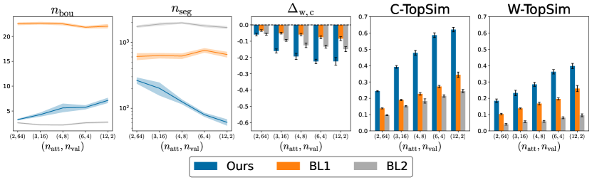
Figure 2: Results for $n_{\textrm{bou}}$, $n_{\textrm{seg}}$, $\Delta_{\textrm{w},\textrm{c}}$, C-TopSim, and W-TopSim are shown in order from the left. The x-axis represents $(n_{\textrm{att}},n_{\textrm{val}})$ while the y-axis represents the values of each metric. The shaded regions and error bars represent the standard error of mean.

We show the results in Figure 2. The results for $n_{\textrm{bou}}$, $n_{\textrm{seg}}$, $\Delta_{\textrm{w},\textrm{c}}$, C-TopSim, and W-TopSim are shown in order from the left. The x-axis represents the $(n_{\textrm{att}},n_{\textrm{val}})$ configurations, while the y-axis represents the values of each metric. As will be explained below, it can be observed that the meaningfulness of segments in emergent language improves when using our objective $\mathcal{J}_{\textrm{ours}}$.

Criteria C1 and C2 are satisfied with $\mathcal{J}_{\textrm{ours}}$: First, see the result for $n_{\textrm{bou}}$ in Figure 2. It is evident that the graph monotonically increases only when the objective $\mathcal{J}_{\textrm{ours}}$ is used. It means that, as $n_{\textrm{att}}$ increases, $n_{\textrm{bou}}$ also increases only when using the objective $\mathcal{J}_{\textrm{ours}}$, confirming that condition C1 is satisfied. Next, see the result for $n_{\textrm{seg}}$ in Figure 2. Again, it is evident that the graph monotonically decreases only when using the objective function $\mathcal{J}_{\textrm{ours}}$. That is, as $n_{\textrm{val}}$ increases, $n_{\textrm{seg}}$ also increases only when using the objective $\mathcal{J}_{\textrm{ours}}$, confirming that condition C2 is satisfied.

Criterion C3 is not met but TopSim per se improved: Refer to the results of $\Delta_{\textrm{w},\textrm{c}}$ in Figure 2. $\Delta_{\textrm{w},\textrm{c}}$ is negative regardless of the objective used. Even when using $\mathcal{J}_{\textrm{ours}}$, condition C3 is not satisfied. However, observe the results for C-TopSim and W-TopSim in Figure 2. By adopting our objective $\mathcal{J}_{\textrm{ours}}$, both C-TopSim and W-TopSim have improved. Notably, the improvement in W-TopSim indicates that the meaningfulness of segments has improved to some extent. $\Delta_{\textrm{w},\textrm{c}}$ does not become positive since C-TopSim has increased even more. We speculate that one reason for $\Delta_{\textrm{w},\textrm{c}}<0$ might be due to the “spelling variation” of segments.

5 Discussion

In Section 3, we proposed formulating the signaling game objective as ELBO and discussed supporting scenarios. In particular, we suggested that prior distributions can influence whether emergent languages follow ZLA. In Section 4, we demonstrated the improvement of segments’ meaningfulness in terms of HAS, with a learnable prior distribution (neural language model).

Why Did Segments Become More Meaningful? We conjecture that the improvement of segments’ meaningfulness is due to the competing pressure of the reconstruction and surprisal term. A receiver wants to be “surprised” because of the reconstruction term. Recall that objects contain $n_{\textrm{att}}$ statistically independent components, i.e., attributes. The receiver must be surprised several times $\propto n_{\textrm{att}}$ to reconstruct the object from a sequential message. At the same time, the receiver does not want to be “surprised” because of the surprisal term. Recall that, in natural language, branching entropy (Eq. 5) decreases on average, but there are some spikes indicating boundaries. In other words, the next character should often be predictable (less surprising), while boundaries appear at points where predictions are hard. The conventional objective $\mathcal{J}_{\textrm{conv}}$ does not contain any incentives to make characters “often predictable,” whereas the surprisal term in ELBO provides the appropriate incentive.

Limitation and Future Work: A populated signaling game (Chaabouni et al., 2022; Rita et al., 2022a; Michel et al., 2023) that involves multiple senders and receivers is important from a sociolinguistic perspective (Raviv et al., 2019). Defining a reasonable ELBO for such a setting is our future work. Perhaps it would be similar to multi-view VAE (Suzuki & Matsuo, 2022). Another remaining task is to extend our generative perspective to discrimination games for which the objective is not reconstructive but contrastive, such as InfoNCE (van den Oord et al., 2018). Furthermore, although we adopted GRU as a prior message distribution, various neural language models have been proposed as cognitive models in computational (psycho)linguistics (Dyer et al., 2016; Shen et al., 2019; Stanojevic et al., 2021; Kuribayashi et al., 2022, inter alia). It should be a key direction to investigate whether such cognitively motivated models give rise to richer structures such as syntax.

6 Related Work

EC as Representation Learning: Several studies regard EC as representation learning (Andreas, 2019; Chaabouni et al., 2020; Xu et al., 2022). For instance, compositionality and disentanglement are often seen as synonymous. TopSim is a representation similarity analysis (RSA, Kriegeskorte et al., 2008), as van der Wal et al. (2020) pointed out. Moreover, Resnick et al. (2020) explicitly formulated the objective as ELBO, though it is not directly applicable to this paper (see footnote 1).

VIB: Tucker et al. (2022) defined a communication game called VQ-VIB, based on Variational Information Bottleneck (VIB, Alemi et al., 2017) which is known as a generalization of beta-VAE. Also, Chaabouni et al. (2021) formalized a color naming game with a similar motivation.

MH Naming Game: Taniguchi et al. (2022) and Inukai et al. (2023) defined a (recursive) MH naming game in which communication was formulated as representation learning on a generative model and emerged through MCMC instead of variational inference.

Natural Language as Prior: Havrylov & Titov (2017) formalized a referential game with a pre-trained natural language model as a prior distribution. Their qualitative evaluation showed that languages became more compositional. Lazaridou et al. (2020) adopted a similar approach.

Dealing with Discreteness: Though we adopted the REINFORCE-like optimization (Mnih & Gregor, 2014) following the previous EC work (Chaabouni et al., 2019; Ueda et al., 2023), there are various approaches dealing with discrete (latent) variables (Rolfe, 2017; Vahdat et al., 2018a, b; Jang et al., 2017; Maddison et al., 2017).

7 Conclusion

In this paper, EC was reinterpreted as representation learning on a generative model. We regarded Lewis’s signaling game as beta-VAE and formulated its objective as ELBO. Our main contributions are (1) to show the similarities between the game and (beta-)VAE, (2) to indicate the impact of prior message distribution on the statistical properties of emergent languages, and (3) to present a computational psycholinguistic interpretation of emergent communication. Specifically, we addressed the issues of Zipf’s law of abbreviation and Harris’s articulation scheme, which had not been reproduced well with the conventional objective. Another important point is that we revisited the variable-length message setting, which previous work often avoided. The remaining tasks for future work are formulating a populated or discrimination game (while keeping the generative viewpoint) and introducing cognitively motivated language models as prior distributions.

Acknowledgments

This work was supported by JSPS KAKENHI Grant Numbers JP21H04904, JP23H04835, and JP23KJ0768.

Appendix A HAS-based Boundary Detection Algorithm

Algorithm 1 Boundary Detection Algorithm

1:$i\leftarrow 0;~{}w\leftarrow 1;~{}\mathcal{B}\leftarrow\{\}$

2:while $i<n$ do

3:     Compute $\textrm{BE}(s_{i:i+w-1})$

4:     if $\textrm{BE}(s_{i:i+w-1})-\textrm{BE}(s_{i:i+w-2})>\textrm{threshold}$ & $w>1$ then

5:         $\mathcal{B}\leftarrow\mathcal{B}\cup\{i+w\}$

6:     end if

7:     if $i+w<n-1$ then

8:         $w\leftarrow w+1$

9:     else

10:         $i\leftarrow i+1;~{}w\leftarrow 1$

11:     end if

12:end while

We show the HAS-based boundary detection algorithm (Tanaka-Ishii, 2005; Tanaka-Ishii & Ishii, 2007) in Algorithm 1. Note that this pseudo code is a simplified version by Ueda et al. (2023). $\mathcal{B}$ is a set of boundary positions. threshold is a hyperparameter.

Appendix B Proofs on the Existence of Implicit Priors

Remark 1.

Since $P^{\textrm{prior}}_{\alpha}(m\mid\alpha)\propto\exp(-\alpha|m|)$ by definition,

$$P^{\textrm{prior}}_{\alpha}(m\mid\alpha)=\frac{1}{Z_{\alpha}}\exp(-\alpha|m|),$$

where $Z_{\alpha}$ is a normalizer to ensure that $P^{\textrm{prior}}_{\alpha}(M\mid\alpha)$ is a probability distribution. $Z_{\alpha}$ can be written as follows:

$$Z_{\alpha} =\sum\nolimits_{m\in\mathcal{M}}\exp(-\alpha|m|)$$

$$=\exp(-\alpha)\sum\nolimits_{l=1}^{L_{\textrm{max}}}\{(|\mathcal{A}|-1)\exp(-\alpha)\}^{l-1} (\text{There are $(|\mathcal{A}|-1)^{l-1}$ messages of length $l$.})$$

$$=\exp(-\alpha)\frac{1-\{(|\mathcal{A}|-1)\exp(-\alpha)\}^{L_{\textrm{max}}}}{1-(|\mathcal{A}|-1)\exp(-\alpha)}$$

$$=\frac{1-\{(|\mathcal{A}|-1)\exp(-\alpha)\}^{L_{\textrm{max}}}}{\exp(\alpha)-|\mathcal{A}|+1}.$$

B.1 Proof of Eq. 9 and Eq. 11

Proof.

As $P^{\textrm{prior}}_{\textrm{unif}}(M)$ is a special case of $P^{\textrm{prior}}_{\alpha}(M\mid\alpha)$, it is sufficient to prove Eq. 11. On the one hand, the left-hand side of Eq. 11 can be transformed as follows:

$$\mathrel{\phantom{=}}\nabla_{\bm{\phi},\bm{\theta}}\mathcal{J}_{\textrm{conv}}(\bm{\phi},\bm{\theta};\alpha)$$

$$=\nabla_{\bm{\phi},\bm{\theta}}\mathbb{E}_{x\sim P_{\textrm{obj}}(\cdot),m\sim S_{\bm{\phi}}(\cdot|x)}[\log R_{\bm{\theta}}(x|m)-\alpha|m|]$$

(By definition)

$$=\mathbb{E}_{x\sim P_{\textrm{obj}}(\cdot),m\sim S_{\bm{\phi}}(\cdot|x)}[\nabla_{\bm{\phi},\bm{\theta}}\log R_{\bm{\theta}}(x|m)-\alpha\nabla_{\bm{\phi},\bm{\theta}}|m|+\{\log R_{\bm{\theta}}(x|m)-\alpha|m|\}\nabla_{\bm{\phi},\bm{\theta}}S_{\bm{\phi}}(m|x)]$$

(By the stochastic computation graph approach (Schulman et al., 2015))

$$=\mathbb{E}_{x\sim P_{\textrm{obj}}(\cdot),m\sim S_{\bm{\phi}}(\cdot|x)}[\nabla_{\bm{\phi},\bm{\theta}}\log R_{\bm{\theta}}(x|m)+\{\log R_{\bm{\theta}}(x|m)-\alpha|m|\}\nabla_{\bm{\phi},\bm{\theta}}S_{\bm{\phi}}(m\mid x)].$$

($$\because\nabla_{\bm{\phi},\bm{\theta}}|m|=0$$)

On the other hand, the right-hand side of Eq. 11 can be transformed as follows:

$$\mathrel{\phantom{=}}\nabla_{\bm{\phi},\bm{\theta}}\mathbb{E}_{x\sim P_{\textrm{obj}}(\cdot),m\sim S_{\bm{\phi}}(\cdot\mid x)}[\log P_{\bm{\theta},\alpha}^{\textrm{joint}}(x,m\mid\alpha)]$$

$$=\nabla_{\bm{\phi},\bm{\theta}}\mathbb{E}_{x\sim P_{\textrm{obj}}(\cdot),m\sim S_{\bm{\phi}}(\cdot|x)}[\log R_{\bm{\theta}}(x\mid m)+\log P^{\textrm{prior}}_{\alpha}(m\mid\alpha)]$$

(By definition)

$$=\mathbb{E}_{x\sim P_{\textrm{obj}}(\cdot),m\sim S_{\bm{\phi}}(\cdot|x)}[$$

$$\mathrel{\phantom{=}}\nabla_{\bm{\phi},\bm{\theta}}\log\!R_{\bm{\theta}}(x|m){+}\nabla_{\bm{\phi},\bm{\theta}}\log\!P^{\textrm{prior}}_{\alpha}(m|\alpha){+}\{\log\!R_{\bm{\theta}}(x|m){+}\log\!P^{\textrm{prior}}_{\alpha}(m|\alpha)\}\nabla_{\bm{\phi},\bm{\theta}}\log\!S_{\bm{\phi}}(m|x)]$$

(By the stochastic computation graph approach (Schulman et al., 2015))

$$=\mathbb{E}_{x\sim P_{\textrm{obj}}(\cdot),m\sim S_{\bm{\phi}}(\cdot|x)}[$$

$$\mathrel{\phantom{=}}\nabla_{\bm{\phi},\bm{\theta}}\log R_{\bm{\theta}}(x\mid m)+\{\log R_{\bm{\theta}}(x\mid m)-\alpha|m|-\log Z_{\alpha}\}\nabla_{\bm{\phi},\bm{\theta}}\log S_{\bm{\phi}}(m\mid x)]$$

($$\because\nabla_{\bm{\phi},\bm{\theta}}\log P^{\textrm{prior}}_{\alpha}(m\mid\alpha)=0 \log P^{\textrm{prior}}_{\alpha}(m\mid\alpha)=-\alpha|m|-\log Z_{\alpha}$$ and )

$$=\mathbb{E}_{x\sim P_{\textrm{obj}}(\cdot),m\sim S_{\bm{\phi}}(\cdot|x)}[\nabla_{\bm{\phi},\bm{\theta}}\log R_{\bm{\theta}}(x\mid m)+\{\log R_{\bm{\theta}}(x\mid m)-\alpha|m|\}\nabla_{\bm{\phi},\bm{\theta}}\log S_{\bm{\phi}}(m\mid x)].$$

($$\because\log Z_{\alpha} m$$ can be seen as a baseline since it does not depend on )

Therefore, Eq. 11 (and its special case Eq. 9) holds. ∎

B.2 Proof of Eq. 15

Proof.

On the one hand, for any message $m=a_{1}\cdots a_{|m|}\in\mathcal{M}$, a monkey typing model can be transformed as follows:

$$\mathrel{\phantom{=}}P^{\textrm{prior}}_{\textrm{monkey}}(m)$$

$$=\prod\nolimits_{t=1}^{|m|}P^{\textrm{prior}}_{\textrm{monkey}}(a_{t}\mid a_{1:t-1})$$ (By definition)

$$=P^{\textrm{prior}}_{\textrm{monkey}}(\texttt{eos}\mid a_{1:|m|-1})\prod\nolimits_{t=1}^{|m|-1}P^{\textrm{prior}}_{\textrm{monkey}}(a_{t}\mid a_{1:t-1})$$ (Only the last symbol is eos)

$$=(1-(|\mathcal{A}|-1)\exp(-\alpha))\exp(-\alpha(|m|-1))$$ (By definition)

$$=(\exp(\alpha)-|\mathcal{A}|+1)\exp(-\alpha|m|).$$

On the other hand, from remark 1, we have:

$$Z_{\alpha}=\frac{1-\{(|\mathcal{A}|-1)\exp(-\alpha)\}^{L_{\textrm{max}}}}{\exp(\alpha)-|\mathcal{A}|+1}\xrightarrow[]{L_{\textrm{max}}\to\infty}\frac{1}{\exp(\alpha)-|\mathcal{A}|+1},$$

when $\alpha>\log(|\mathcal{A}|-1)$. Therefore, we have:

$$P^{\textrm{prior}}_{\alpha}(m\mid\alpha)=\frac{\exp(-\alpha|m|)}{Z_{\mathcal{A}}}\xrightarrow{L_{\textrm{max}}\to\infty}(\exp(\alpha)-|\mathcal{A}|+1)\exp(-\alpha|m|)=P^{\textrm{prior}}_{\textrm{monkey}}(m)$$

when $\alpha>\log(|\mathcal{A}|-1)$. ∎

Remark 2.

In fact, it has been shown (Miller, 1957; Conrad & Mitzenmacher, 2004) that even the monkey typing model $P^{\textrm{prior}}_{\textrm{monkey}}(m)$ follows ZLA.

B.3 Proof of Eq. 13

Proof.

First, $\mathcal{J}_{\textrm{elbo}}(\bm{\phi},\bm{\theta};\alpha)$ can be transformed as follows:

$$\mathrel{\phantom{:=}}\mathcal{J}_{\textrm{elbo}}(\bm{\phi},\bm{\theta};\alpha)$$

$$=\mathbb{E}_{x\sim P_{\textrm{obj}}(\cdot)}[\mathbb{E}_{m\sim S_{\bm{\phi}}(\cdot|x)}[\log R_{\bm{\theta}}(x\mid m)]-D_{\mathrm{KL}}(S_{\bm{\phi}}(Mmx)||P^{\textrm{prior}}_{\alpha}(Mm\alpha))]$$

(By definition)

$$=\mathbb{E}_{x\sim P_{\textrm{obj}}(\cdot)}[\mathbb{E}_{m\sim S_{\bm{\phi}}(\cdot|x)}[\log R_{\bm{\theta}}(x\mid m)]-\mathbb{E}_{m\sim S_{\bm{\phi}}(\cdot|x)}[\log S_{\bm{\phi}}(m\mid x)-\log P^{\textrm{prior}}_{\alpha}(m\mid\alpha)]]$$

(By the definition of $$D_{\mathrm{KL}}$$)

$$=\mathbb{E}_{x\sim P_{\textrm{obj}}(\cdot),m\sim S_{\bm{\phi}}(\cdot|x)}[\log R_{\bm{\theta}}(x\mid m)+\log P^{\textrm{prior}}_{\alpha}(m)]-\mathbb{E}_{x\sim P_{\textrm{obj}}(\cdot),m\sim S_{\bm{\phi}}(\cdot|x)}[\log S_{\bm{\phi}}(m\mid x)]$$

(By the linearity of $$\mathbb{E}$$)

$$=\mathbb{E}_{x\sim P_{\textrm{obj}}(\cdot),m\sim S_{\bm{\phi}}(\cdot|x)}[\log R_{\bm{\theta}}(x\mid m)+\log P^{\textrm{prior}}_{\alpha}(m)]-\mathbb{E}_{x\sim P_{\textrm{obj}}(\cdot)}[\mathcal{H}(S_{\bm{\phi}}(M\mid x))]$$

(By the definition of $$\mathcal{H}$$)

$$=\mathbb{E}_{x\sim P_{\textrm{obj}}(\cdot),m\sim S_{\bm{\phi}}(\cdot|x)}[\log R_{\bm{\theta}}(x\mid m)-\alpha|m|]+\mathbb{E}_{x\sim P_{\textrm{obj}}(\cdot)}[\mathcal{H}(S_{\bm{\phi}}(M\mid x))]-\log Z_{\alpha}$$

(By the definition of $$P^{\textrm{prior}}_{\alpha}$$)

$$=\mathcal{J}_{\textrm{conv}}(\bm{\phi},\bm{\theta};\alpha)+\beta\mathbb{E}_{x\sim P_{\textrm{obj}}(\cdot)}[\mathcal{H}(S_{\bm{\phi}}(M\mid x))]-\log Z_{\alpha}.$$

(By the definition of $$\mathcal{J}_{\textrm{conv}}(\bm{\phi},\bm{\theta};\alpha)$$)

Thus,

$$\mathrel{\phantom{=}}\nabla_{\bm{\phi},\bm{\theta}}\mathcal{J}_{\textrm{elbo}}(\bm{\phi},\bm{\theta};\alpha)$$

$$=\nabla_{\bm{\phi},\bm{\theta}}\mathcal{J}_{\textrm{conv}}(\bm{\phi},\bm{\theta};\alpha)+\nabla_{\bm{\phi},\bm{\theta}}\mathbb{E}_{x\sim P_{\textrm{obj}}(\cdot)}[\mathcal{H}(S_{\bm{\phi}}(M\mid x))]-\underbrace{\nabla_{\bm{\phi},\bm{\theta}}\log Z_{\alpha}}_{=0}$$

$$=\nabla_{\bm{\phi},\bm{\theta}}\mathcal{J}_{\textrm{conv}}(\bm{\phi},\bm{\theta};\alpha)+\nabla_{\bm{\phi},\bm{\theta}}\mathbb{E}_{x\sim P_{\textrm{obj}}(\cdot)}[\mathcal{H}(S_{\bm{\phi}}(M\mid x))].$$

∎

Appendix C Supplemental Information on Experimental Setup

Sender Architecture: The sender $S_{\bm{\phi}}$ is based on GRU (Cho et al., 2014) with hidden states of size $512$ and has embedding layers converting symbols to $32$-dimensional vectors. In addition, LayerNorm (Ba et al., 2016) is applied to the hidden states and embeddings for faster convergence. For $t\geq 0$,

$$\bm{e}_{\bm{\phi},t} =\begin{cases}\bm{\phi}_{\texttt{bos}}&(t=0)\\ \textrm{Embedding}(m_{t};\bm{\phi}_{\textrm{s-emb}})&(t>0)\end{cases},$$ (18)

$$\bm{e}_{\bm{\phi},t}^{\textrm{LN}} =\textrm{LayerNorm}(\bm{e}_{t}),$$

$$\bm{h}_{\bm{\phi},t} =\begin{cases}\textrm{Encoder}(x;\bm{\phi}_{\textrm{o-emb}})&(t=0)\\ \textrm{GRU}(\bm{e}_{t-1}^{\textrm{LN}},\bm{h}_{t-1}^{\textrm{LN}};\bm{\phi}_{\textrm{gru}})&(t>0)\end{cases},$$

$$\bm{h}_{\bm{\phi},t}^{\textrm{LN}} =\textrm{LayerNorm}(\bm{h}_{t}),$$

where $\bm{\phi}_{\texttt{bos}},\bm{\phi}_{\textrm{s-emb}},\bm{\phi}_{\textrm{o-emb}},\bm{\phi}_{\textrm{gru}}\in\bm{\phi}$. The object encoder is represented as the additive composition of the embedding layers of attributes. The sender $S_{\bm{\phi}}$ also has the linear layer (with bias) to predict the next symbol. For $t\geq 0$,

$$S_{\bm{\phi}}(A_{t+1}\mid m_{1:t}) =\textrm{Softmax}(\bm{W}_{S}\bm{h}_{\bm{\phi},t}^{\textrm{LN}}+\bm{b}_{S}),$$ (19)

where $\bm{W}_{S},\bm{b}_{S}\in\bm{\phi}$.

Receiver Architecture: The receiver has a similar architecture to the sender. The receiver $R_{\bm{\theta}}$ is based on GRU (Cho et al., 2014) with hidden states of size $512$ and has embedding layers converting symbols to $32$-dimensional vectors. In addition, LayerNorm (Ba et al., 2016) and Gaussian dropout (Srivastava et al., 2014) are applied to the hidden states and embeddings. The dropout scale is set to $0.001$. For $t\geq 0$,

$$\bm{e}_{\bm{\theta},t} =\begin{cases}\bm{\theta}_{\texttt{bos}}&(t=0)\\ \textrm{Embedding}(m_{t};\bm{\theta}_{\textrm{s-emb}})&(t>0)\end{cases},$$ (20)

$$\bm{e}_{\bm{\theta},t}^{\textrm{LN}} =\textrm{LayerNorm}(\bm{e}_{t}\odot\bm{d}_{e}),$$

$$\bm{h}_{\bm{\theta},t} =\begin{cases}\bm{0}&(t=0)\\ \textrm{GRU}(\bm{e}_{t-1}^{\textrm{LN}},\bm{h}_{t-1}^{\textrm{LN}};\bm{\theta}_{\textrm{gru}})&(t>0)\end{cases},$$

$$\bm{h}_{\bm{\theta},t}^{\textrm{LN}} =\textrm{LayerNorm}(\bm{h}_{t}\odot\bm{d}_{h}),$$

where $\bm{\theta}_{\texttt{bos}},\bm{\theta}_{\textrm{s-emb}},\bm{\theta}_{\textrm{o-emb}},\bm{\theta}_{\textrm{gru}}\in\bm{\theta}$, $\odot$ is Hadamard product, and $\bm{d}_{e},\bm{d}_{h}$ are dropout masks. Note that the dropout masks are fixed over time $t$, following Gal & Ghahramani (2016). The receiver $R_{\bm{\theta}}$ also has the linear layer (with bias) to predict the next symbol. For $t\geq 0$,

$$R_{\bm{\theta}}(A_{t+1}\mid m_{1:t}) =\textrm{Softmax}(\bm{W}_{R}\bm{h}_{\bm{\theta},t}^{\textrm{LN}}+\bm{b}_{R}),$$ (21)

where $\bm{W}_{R},\bm{b}_{R}\in\bm{\theta}$.

Optimization: We have to optimize ELBO in which latent variables are discrete sequences, similarly to Mnih & Gregor (2014). By the stochastic computation approach (Schulman et al., 2015), we obtain the following surrogate objective:

$$\mathcal{J}_{\textrm{surrogate}}(\bm{\phi},\bm{\theta}) :=\log R_{\bm{\theta}}(x\mid m)+\beta\sum\nolimits_{t=1}^{|m|}\log P^{\textrm{prior}}_{\bm{\theta}}(m_{t}\mid m_{1:t-1})$$ (22)

$$\mathrel{\phantom{:=}}+\sum\nolimits_{t=1}^{|m|}\textrm{StopGrad}(C_{\bm{\phi},\bm{\theta},t}-B_{\bm{\zeta}}(x,m_{1:t-1}))\log S_{\bm{\phi}}(m_{t}\mid x,m_{1:t-1}),$$

where $\textrm{StopGrad}(\cdot)$ is the stop-gradient operator, $B_{\bm{\zeta}}(x,m_{1:t-1})$ is a state-dependent baseline parametrized by $\bm{\zeta}$, and

$$C_{\bm{\phi},\bm{\theta},t}=\log R_{\bm{\theta}}(x\mid m)+\beta\sum\nolimits_{u=t}^{|m|}(\log P^{\textrm{prior}}_{\bm{\theta}}(m_{u}\mid m_{1:u-1})-\log S_{\bm{\phi}}(m_{u}\mid x,m_{1:u-1})).$$

The architecture of the baseline $B(x,m_{1:t-1})$ is defined as:

$$B(x,m_{1:t-1})=B(\bm{h}_{\bm{\phi},t}^{\textrm{LN}})=\bm{w}_{B,2}^{\top}\textrm{LeakyReLU}(\bm{W}_{B,1}\textrm{StopGrad}(\bm{h}_{\bm{\phi},t}^{\textrm{LN}})+\bm{b}_{B,1})+b_{B,2},$$

where $\bm{W}_{B,1}\in\mathbb{R}^{256\times 512},\bm{b}_{B,1}\in\mathbb{R}^{256},\bm{w}_{B,2}\in\mathbb{R}^{256},b_{B,2}\in\mathbb{R}$ are learnable parameters in $\bm{\zeta}$. We optimize the baseline’s parameter $\bm{\zeta}$ by simultaneously minimizing the sum of square errors:

$$\mathcal{J}_{\textrm{baseline}}(\bm{\zeta}):=\sum\nolimits_{t=1}^{|m|}(C_{t}-B_{\bm{\zeta}}(x,m_{1:t-1}))^{2}.$$ (23)

Note that we optimize the sender’s parameter $\bm{\phi}$ according to $\mathcal{J}_{\textrm{surrogate}}$ but not $\mathcal{J}_{\textrm{baseline}}$, so as not to break the original problem setting of ELBO maximization w.r.t $\bm{\phi},\bm{\theta}$. We use Adam (Kingma & Ba, 2015) as an optimizer. The learning rate is set to $10^{-4}$. The batch size is set to $8192$. The parameters are updated $20000$ times for each run. To avoid posterior collapse, $\beta$ is initially set $\ll 1$ and annealed to $1$ via the REWO algorithm (Klushyn et al., 2019). We set the constraint parameter of REWO to $0.3$, which intuitively means that it tries to bring $\beta$ closer to $1$ while trying to keep the exponential moving average of the reconstruction error $-\log R_{\bm{\theta}}(x\mid m)$ less than $0.3$.In the conventional setting, Rita et al. (2020) adopted the ad-hoc annealing of the length-penalty coefficient $\alpha$. It might roughly correspond to $\beta$-annealing in VAE.

Appendix D Supplemental Information on Experimental Result

Figure 3: Results for $n_{\textrm{bou}}$, $n_{\textrm{seg}}$, $\Delta_{\textrm{w},\textrm{c}}$, C-TopSim, and W-TopSim are shown in order from the left. The x-axis represents $(n_{\textrm{att}},n_{\textrm{val}})$ while the y-axis represents the values of each metric. The shaded regions and error bars represent the standard error of mean. threshold is set to 0.25.

Figure 4: Results for $n_{\textrm{bou}}$, $n_{\textrm{seg}}$, $\Delta_{\textrm{w},\textrm{c}}$, C-TopSim, and W-TopSim are shown in order from the left. The x-axis represents $(n_{\textrm{att}},n_{\textrm{val}})$ while the y-axis represents the values of each metric. The shaded regions and error bars represent the standard error of mean. threshold is set to 0.5. Criterion C2 is a bit violated. So this threshold is not appropriate.

Appendix E Supplemental Experiment on Zipf’s law of abbreviation

E.1 Setup

Object and Message Space: We set $\mathcal{X}:=\{1,\ldots,1000\}$, $P_{\textrm{obj}}(x)\propto x^{-1}$, $L_{\textrm{max}}=30$, and $|\mathcal{A}|\in\{5,10,20,30,40\}$ following (Chaabouni et al., 2019).

Agent Architectures and Optimization: The architectures of sender $S_{\bm{\phi}}$ and $R_{\bm{\theta}}$ are the same as described in Section 4.1. The optimization method and parameters are also the same as described in Section 4.1.

E.2 Result and Discussion

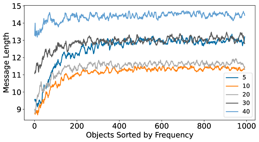
Figure 5: Mean message length sorted by objects’ frequency across 32 random seeds. For readability, a moving average with a window size of 10 is shown.

The experimental results are shown in Figure 5. As can be seen from the figure, there is a tendency for shorter messages to be assigned to high-frequency objects.

It is also observed that the larger the alphabet size $|\mathcal{A}|$, the longer the messages tend to be. It is probably because, as the alphabet size $|\mathcal{A}|$ increases, the likelihood of eos becomes smaller in the early stages of training.

As an intuitive analogy for this, let us assume that a sender $S_{\bm{\phi}}(M|X)$ and prior message distribution $P^{\textrm{prior}}_{\bm{\theta}}(M)$ are roughly similar to a uniform monkey typing (UMT) in the early stages of training:

$$S_{\bm{\phi}}(m_{t}\mid x,m_{1:t-1})\approx\frac{1}{|\mathcal{A}|},\quad P^{\textrm{prior}}_{\bm{\theta}}(m_{t}\mid m_{1:t-1})\approx\frac{1}{|\mathcal{A}|}.$$ (24)

The length distribution of UMT is a geometry distribution with a parameter $p=|\mathcal{A}|^{-1}$ (Imagine a situation where you roll the dice with “eos” written on one face until you get that face). Then, the expected message length of UMT is $p^{-1}=|\mathcal{A}|$. Therefore, as the alphabet size $|\mathcal{A}|$ increases, the sender $S_{\bm{\phi}}(M|X)$ and prior message distribution $P^{\textrm{prior}}_{\bm{\theta}}(M)$ are inclined to prefer longer messages in the early stages. Consequently, they are more likely to converge to longer messages. Designing neural network architectures that maintain a consistent scale for eos regardless of alphabet size is a challenge for future work.

References

- Alemi et al. (2017) Alexander A. Alemi, Ian Fischer, Joshua V. Dillon, and Kevin Murphy. Deep variational information bottleneck. In 5th International Conference on Learning Representations, ICLR 2017, Toulon, France, April 24-26, 2017, Conference Track Proceedings. OpenReview.net, 2017. URL https://openreview.net/forum?id=HyxQzBceg.
- Alemi et al. (2018) Alexander A. Alemi, Ben Poole, Ian Fischer, Joshua V. Dillon, Rif A. Saurous, and Kevin Murphy. Fixing a broken ELBO. In Jennifer G. Dy and Andreas Krause (eds.), Proceedings of the 35th International Conference on Machine Learning, ICML 2018, Stockholmsmässan, Stockholm, Sweden, July 10-15, 2018, volume 80 of Proceedings of Machine Learning Research, pp. 159–168. PMLR, 2018. URL http://proceedings.mlr.press/v80/alemi18a.html.
- Andreas (2019) Jacob Andreas. Measuring compositionality in representation learning. In 7th International Conference on Learning Representations, ICLR 2019, New Orleans, LA, USA, May 6-9, 2019. OpenReview.net, 2019. URL https://openreview.net/forum?id=HJz05o0qK7.
- Ba et al. (2016) Lei Jimmy Ba, Jamie Ryan Kiros, and Geoffrey E. Hinton. Layer normalization. CoRR, abs/1607.06450, 2016. URL http://arxiv.org/abs/1607.06450.
- Bell et al. (1990) Timothy C. Bell, John G. Cleary, and Ian H. Witten. Text Compression. Prentice-Hall, Inc., 1990.
- Bowman et al. (2016) Samuel R. Bowman, Luke Vilnis, Oriol Vinyals, Andrew M. Dai, Rafal Józefowicz, and Samy Bengio. Generating sentences from a continuous space. In Yoav Goldberg and Stefan Riezler (eds.), Proceedings of the 20th SIGNLL Conference on Computational Natural Language Learning, CoNLL 2016, Berlin, Germany, August 11-12, 2016, pp. 10–21. ACL, 2016. doi: 10.18653/v1/k16-1002. URL https://doi.org/10.18653/v1/k16-1002.
- Brandizzi (2023) Nicolo’ Brandizzi. Towards more human-like AI communication: A review of emergent communication research. CoRR, abs/2308.02541, 2023. doi: 10.48550/arXiv.2308.02541. URL https://doi.org/10.48550/arXiv.2308.02541.
- Brighton & Kirby (2006) Henry Brighton and Simon Kirby. Understanding linguistic evolution by visualizing the emergence of topographic mappings. Artif. Life, 12(2):229–242, 2006. URL https://doi.org/10.1162/artl.2006.12.2.229.
- Chaabouni et al. (2019) Rahma Chaabouni, Eugene Kharitonov, Emmanuel Dupoux, and Marco Baroni. Anti-efficient encoding in emergent communication. In Hanna M. Wallach, Hugo Larochelle, Alina Beygelzimer, Florence d’Alché-Buc, Emily B. Fox, and Roman Garnett (eds.), Advances in Neural Information Processing Systems 32: Annual Conference on Neural Information Processing Systems 2019, NeurIPS 2019, December 8-14, 2019, Vancouver, BC, Canada, pp. 6290–6300, 2019. URL https://proceedings.neurips.cc/paper/2019/hash/31ca0ca71184bbdb3de7b20a51e88e90-Abstract.html.
- Chaabouni et al. (2020) Rahma Chaabouni, Eugene Kharitonov, Diane Bouchacourt, Emmanuel Dupoux, and Marco Baroni. Compositionality and generalization in emergent languages. In Dan Jurafsky, Joyce Chai, Natalie Schluter, and Joel R. Tetreault (eds.), Proceedings of the 58th Annual Meeting of the Association for Computational Linguistics, ACL 2020, Online, July 5-10, 2020, pp. 4427–4442. Association for Computational Linguistics, 2020. URL https://doi.org/10.18653/v1/2020.acl-main.407.
- Chaabouni et al. (2021) Rahma Chaabouni, Eugene Kharitonov, Emmanuel Dupoux, and Marco Baroni. Communicating artificial neural networks develop efficient color-naming systems. Proceedings of the National Academy of Sciences, 118(12):e2016569118, 2021. doi: 10.1073/pnas.2016569118. URL https://www.pnas.org/doi/abs/10.1073/pnas.2016569118.
- Chaabouni et al. (2022) Rahma Chaabouni, Florian Strub, Florent Altché, Eugene Tarassov, Corentin Tallec, Elnaz Davoodi, Kory Wallace Mathewson, Olivier Tieleman, Angeliki Lazaridou, and Bilal Piot. Emergent communication at scale. In The Tenth International Conference on Learning Representations, ICLR 2022, Virtual Event, April 25-29, 2022. OpenReview.net, 2022. URL https://openreview.net/forum?id=AUGBfDIV9rL.
- Cho et al. (2014) Kyunghyun Cho, Bart van Merrienboer, Çaglar Gülçehre, Dzmitry Bahdanau, Fethi Bougares, Holger Schwenk, and Yoshua Bengio. Learning phrase representations using RNN encoder-decoder for statistical machine translation. In Alessandro Moschitti, Bo Pang, and Walter Daelemans (eds.), Proceedings of the 2014 Conference on Empirical Methods in Natural Language Processing, EMNLP 2014, October 25-29, 2014, Doha, Qatar, A meeting of SIGDAT, a Special Interest Group of the ACL, pp. 1724–1734. ACL, 2014. URL https://doi.org/10.3115/v1/d14-1179.
- Choi et al. (2018) Edward Choi, Angeliki Lazaridou, and Nando de Freitas. Compositional obverter communication learning from raw visual input. In 6th International Conference on Learning Representations, ICLR 2018, Vancouver, BC, Canada, April 30 - May 3, 2018, Conference Track Proceedings. OpenReview.net, 2018. URL https://openreview.net/forum?id=rknt2Be0-.
- Conrad & Mitzenmacher (2004) Brian Conrad and Michael Mitzenmacher. Power laws for monkeys typing randomly: the case of unequal probabilities. IEEE Transactions on Information Theory, 50(7):1403–1414, 2004. doi: 10.1109/TIT.2004.830752.
- Cover & Thomas (2006) Thomas M. Cover and Joy A. Thomas. Elements of Information Theory (Wiley Series in Telecommunications and Signal Processing). Wiley-Interscience, 2006.
- Deng et al. (2009) Jia Deng, Wei Dong, Richard Socher, Li-Jia Li, Kai Li, and Li Fei-Fei. Imagenet: A large-scale hierarchical image database. In 2009 IEEE Computer Society Conference on Computer Vision and Pattern Recognition (CVPR 2009), 20-25 June 2009, Miami, Florida, USA, pp. 248–255. IEEE Computer Society, 2009. doi: 10.1109/CVPR.2009.5206848. URL https://doi.org/10.1109/CVPR.2009.5206848.
- Dessì et al. (2021) Roberto Dessì, Eugene Kharitonov, and Marco Baroni. Interpretable agent communication from scratch (with a generic visual processor emerging on the side). In Marc’Aurelio Ranzato, Alina Beygelzimer, Yann N. Dauphin, Percy Liang, and Jennifer Wortman Vaughan (eds.), Advances in Neural Information Processing Systems 34: Annual Conference on Neural Information Processing Systems 2021, NeurIPS 2021, December 6-14, 2021, virtual, pp. 26937–26949, 2021. URL https://proceedings.neurips.cc/paper/2021/hash/e250c59336b505ed411d455abaa30b4d-Abstract.html.
- Dyer et al. (2016) Chris Dyer, Adhiguna Kuncoro, Miguel Ballesteros, and Noah A. Smith. Recurrent neural network grammars. In Kevin Knight, Ani Nenkova, and Owen Rambow (eds.), NAACL HLT 2016, The 2016 Conference of the North American Chapter of the Association for Computational Linguistics: Human Language Technologies, San Diego California, USA, June 12-17, 2016, pp. 199–209. The Association for Computational Linguistics, 2016. doi: 10.18653/v1/n16-1024. URL https://doi.org/10.18653/v1/n16-1024.
- Foerster et al. (2016) Jakob N. Foerster, Yannis M. Assael, Nando de Freitas, and Shimon Whiteson. Learning to communicate with deep multi-agent reinforcement learning. In Daniel D. Lee, Masashi Sugiyama, Ulrike von Luxburg, Isabelle Guyon, and Roman Garnett (eds.), Advances in Neural Information Processing Systems 29: Annual Conference on Neural Information Processing Systems 2016, December 5-10, 2016, Barcelona, Spain, pp. 2137–2145, 2016. URL https://proceedings.neurips.cc/paper/2016/hash/c7635bfd99248a2cdef8249ef7bfbef4-Abstract.html.
- Fu et al. (2019) Hao Fu, Chunyuan Li, Xiaodong Liu, Jianfeng Gao, Asli Celikyilmaz, and Lawrence Carin. Cyclical annealing schedule: A simple approach to mitigating KL vanishing. In Jill Burstein, Christy Doran, and Thamar Solorio (eds.), Proceedings of the 2019 Conference of the North American Chapter of the Association for Computational Linguistics: Human Language Technologies, NAACL-HLT 2019, Minneapolis, MN, USA, June 2-7, 2019, Volume 1 (Long and Short Papers), pp. 240–250. Association for Computational Linguistics, 2019. doi: 10.18653/v1/n19-1021. URL https://doi.org/10.18653/v1/n19-1021.
- Gal & Ghahramani (2016) Yarin Gal and Zoubin Ghahramani. A theoretically grounded application of dropout in recurrent neural networks. In Daniel D. Lee, Masashi Sugiyama, Ulrike von Luxburg, Isabelle Guyon, and Roman Garnett (eds.), Advances in Neural Information Processing Systems 29: Annual Conference on Neural Information Processing Systems 2016, December 5-10, 2016, Barcelona, Spain, pp. 1019–1027, 2016. URL https://proceedings.neurips.cc/paper/2016/hash/076a0c97d09cf1a0ec3e19c7f2529f2b-Abstract.html.
- Galke et al. (2022) Lukas Galke, Yoav Ram, and Limor Raviv. Emergent communication for understanding human language evolution: What’s missing? CoRR, abs/2204.10590, 2022. doi: 10.48550/arXiv.2204.10590. URL https://doi.org/10.48550/arXiv.2204.10590.
- Hale (2001) John Hale. A probabilistic earley parser as a psycholinguistic model. In Language Technologies 2001: The Second Meeting of the North American Chapter of the Association for Computational Linguistics, NAACL 2001, Pittsburgh, PA, USA, June 2-7, 2001. The Association for Computational Linguistics, 2001. URL https://aclanthology.org/N01-1021/.
- Harris (1955) Zellig S. Harris. From phoneme to morpheme. Language, 31(2):190–222, 1955. URL http://www.jstor.org/stable/411036.
- Havrylov & Titov (2017) Serhii Havrylov and Ivan Titov. Emergence of language with multi-agent games: Learning to communicate with sequences of symbols. In Isabelle Guyon, Ulrike von Luxburg, Samy Bengio, Hanna M. Wallach, Rob Fergus, S. V. N. Vishwanathan, and Roman Garnett (eds.), Advances in Neural Information Processing Systems 30: Annual Conference on Neural Information Processing Systems 2017, December 4-9, 2017, Long Beach, CA, USA, pp. 2149–2159, 2017. URL https://proceedings.neurips.cc/paper/2017/hash/70222949cc0db89ab32c9969754d4758-Abstract.html.
- Higgins et al. (2017) Irina Higgins, Loïc Matthey, Arka Pal, Christopher P. Burgess, Xavier Glorot, Matthew M. Botvinick, Shakir Mohamed, and Alexander Lerchner. beta-vae: Learning basic visual concepts with a constrained variational framework. In 5th International Conference on Learning Representations, ICLR 2017, Toulon, France, April 24-26, 2017, Conference Track Proceedings. OpenReview.net, 2017. URL https://openreview.net/forum?id=Sy2fzU9gl.
- Hochreiter & Schmidhuber (1997) Sepp Hochreiter and Jürgen Schmidhuber. Long short-term memory. Neural Comput., 9(8):1735–1780, 1997. URL https://doi.org/10.1162/neco.1997.9.8.1735.
- Inukai et al. (2023) Jun Inukai, Tadahiro Taniguchi, Akira Taniguchi, and Yoshinobu Hagiwara. Recursive metropolis-hastings naming game: Symbol emergence in a multi-agent system based on probabilistic generative models. CoRR, abs/2305.19761, 2023. doi: 10.48550/arXiv.2305.19761. URL https://doi.org/10.48550/arXiv.2305.19761.
- Jang et al. (2017) Eric Jang, Shixiang Gu, and Ben Poole. Categorical reparameterization with gumbel-softmax. In 5th International Conference on Learning Representations, ICLR 2017, Toulon, France, April 24-26, 2017, Conference Track Proceedings. OpenReview.net, 2017. URL https://openreview.net/forum?id=rkE3y85ee.
- Jaques et al. (2019) Natasha Jaques, Angeliki Lazaridou, Edward Hughes, Çaglar Gülçehre, Pedro A. Ortega, DJ Strouse, Joel Z. Leibo, and Nando de Freitas. Social influence as intrinsic motivation for multi-agent deep reinforcement learning. In Kamalika Chaudhuri and Ruslan Salakhutdinov (eds.), Proceedings of the 36th International Conference on Machine Learning, ICML 2019, 9-15 June 2019, Long Beach, California, USA, volume 97 of Proceedings of Machine Learning Research, pp. 3040–3049. PMLR, 2019. URL http://proceedings.mlr.press/v97/jaques19a.html.
- Kharitonov et al. (2020) Eugene Kharitonov, Rahma Chaabouni, Diane Bouchacourt, and Marco Baroni. Entropy minimization in emergent languages. In Proceedings of the 37th International Conference on Machine Learning, ICML 2020, 13-18 July 2020, Virtual Event, volume 119 of Proceedings of Machine Learning Research, pp. 5220–5230. PMLR, 2020. URL http://proceedings.mlr.press/v119/kharitonov20a.html.
- Kingma & Ba (2015) Diederik P. Kingma and Jimmy Ba. Adam: A method for stochastic optimization. In Yoshua Bengio and Yann LeCun (eds.), 3rd International Conference on Learning Representations, ICLR 2015, San Diego, CA, USA, May 7-9, 2015, Conference Track Proceedings, 2015. URL http://arxiv.org/abs/1412.6980.
- Kingma & Welling (2014) Diederik P. Kingma and Max Welling. Auto-encoding variational bayes. In 2nd International Conference on Learning Representations, ICLR 2014, Banff, AB, Canada, April 14-16, 2014, Conference Track Proceedings, 2014. URL http://arxiv.org/abs/1312.6114.
- Kirby et al. (2014) Simon Kirby, Tom Griffiths, and Kenny Smith. Iterated learning and the evolution of language. Current Opinion in Neurobiology, 28:108–114, 2014. ISSN 0959-4388. doi: https://doi.org/10.1016/j.conb.2014.07.014. URL https://www.sciencedirect.com/science/article/pii/S0959438814001421. SI: Communication and language.
- Kirby et al. (2015) Simon Kirby, Monica Tamariz, Hannah Cornish, and Kenny Smith. Compression and communication in the cultural evolution of linguistic structure. Cognition, 141:87–102, 2015. ISSN 0010-0277. doi: https://doi.org/10.1016/j.cognition.2015.03.016. URL https://www.sciencedirect.com/science/article/pii/S0010027715000815.
- Klushyn et al. (2019) Alexej Klushyn, Nutan Chen, Richard Kurle, Botond Cseke, and Patrick van der Smagt. Learning hierarchical priors in vaes. In Hanna M. Wallach, Hugo Larochelle, Alina Beygelzimer, Florence d’Alché-Buc, Emily B. Fox, and Roman Garnett (eds.), Advances in Neural Information Processing Systems 32: Annual Conference on Neural Information Processing Systems 2019, NeurIPS 2019, December 8-14, 2019, Vancouver, BC, Canada, pp. 2866–2875, 2019. URL https://proceedings.neurips.cc/paper/2019/hash/7d12b66d3df6af8d429c1a357d8b9e1a-Abstract.html.
- Kottur et al. (2017) Satwik Kottur, José M. F. Moura, Stefan Lee, and Dhruv Batra. Natural language does not emerge ’naturally’ in multi-agent dialog. In Martha Palmer, Rebecca Hwa, and Sebastian Riedel (eds.), Proceedings of the 2017 Conference on Empirical Methods in Natural Language Processing, EMNLP 2017, Copenhagen, Denmark, September 9-11, 2017, pp. 2962–2967. Association for Computational Linguistics, 2017. URL https://doi.org/10.18653/v1/d17-1321.
- Kriegeskorte et al. (2008) Nikolaus Kriegeskorte, Marieke Mur, and Peter Bandettini. Representational similarity analysis - connecting the branches of systems neuroscience. Frontiers in Systems Neuroscience, 2, 2008. ISSN 1662-5137. doi: 10.3389/neuro.06.004.2008. URL https://www.frontiersin.org/articles/10.3389/neuro.06.004.2008.
- Kuribayashi et al. (2022) Tatsuki Kuribayashi, Yohei Oseki, Ana Brassard, and Kentaro Inui. Context limitations make neural language models more human-like. In Yoav Goldberg, Zornitsa Kozareva, and Yue Zhang (eds.), Proceedings of the 2022 Conference on Empirical Methods in Natural Language Processing, EMNLP 2022, Abu Dhabi, United Arab Emirates, December 7-11, 2022, pp. 10421–10436. Association for Computational Linguistics, 2022. doi: 10.18653/v1/2022.emnlp-main.712. URL https://doi.org/10.18653/v1/2022.emnlp-main.712.
- Lazaridou & Baroni (2020) Angeliki Lazaridou and Marco Baroni. Emergent multi-agent communication in the deep learning era. CoRR, abs/2006.02419, 2020. URL https://arxiv.org/abs/2006.02419.
- Lazaridou et al. (2017) Angeliki Lazaridou, Alexander Peysakhovich, and Marco Baroni. Multi-agent cooperation and the emergence of (natural) language. In 5th International Conference on Learning Representations, ICLR 2017, Toulon, France, April 24-26, 2017, Conference Track Proceedings. OpenReview.net, 2017. URL https://openreview.net/forum?id=Hk8N3Sclg.
- Lazaridou et al. (2018) Angeliki Lazaridou, Karl Moritz Hermann, Karl Tuyls, and Stephen Clark. Emergence of linguistic communication from referential games with symbolic and pixel input. In 6th International Conference on Learning Representations, ICLR 2018, Vancouver, BC, Canada, April 30 - May 3, 2018, Conference Track Proceedings. OpenReview.net, 2018. URL https://openreview.net/forum?id=HJGv1Z-AW.
- Lazaridou et al. (2020) Angeliki Lazaridou, Anna Potapenko, and Olivier Tieleman. Multi-agent communication meets natural language: Synergies between functional and structural language learning. In Dan Jurafsky, Joyce Chai, Natalie Schluter, and Joel R. Tetreault (eds.), Proceedings of the 58th Annual Meeting of the Association for Computational Linguistics, ACL 2020, Online, July 5-10, 2020, pp. 7663–7674. Association for Computational Linguistics, 2020. URL https://doi.org/10.18653/v1/2020.acl-main.685.
- Levine (2018) Sergey Levine. Reinforcement learning and control as probabilistic inference: Tutorial and review. CoRR, abs/1805.00909, 2018. URL http://arxiv.org/abs/1805.00909.
- Levy (2008) Roger Levy. Expectation-based syntactic comprehension. Cognition, 106(3):1126–1177, 2008. ISSN 0010-0277. doi: https://doi.org/10.1016/j.cognition.2007.05.006. URL https://www.sciencedirect.com/science/article/pii/S0010027707001436.
- Lewis (1969) David K. Lewis. Convention: A Philosophical Study. Wiley-Blackwell, 1969.
- Li & Bowling (2019) Fushan Li and Michael Bowling. Ease-of-teaching and language structure from emergent communication. In Hanna M. Wallach, Hugo Larochelle, Alina Beygelzimer, Florence d’Alché-Buc, Emily B. Fox, and Roman Garnett (eds.), Advances in Neural Information Processing Systems 32: Annual Conference on Neural Information Processing Systems 2019, NeurIPS 2019, December 8-14, 2019, Vancouver, BC, Canada, pp. 15825–15835, 2019. URL https://proceedings.neurips.cc/paper/2019/hash/b0cf188d74589db9b23d5d277238a929-Abstract.html.
- Lin et al. (2014) Tsung-Yi Lin, Michael Maire, Serge J. Belongie, James Hays, Pietro Perona, Deva Ramanan, Piotr Dollár, and C. Lawrence Zitnick. Microsoft COCO: common objects in context. In David J. Fleet, Tomás Pajdla, Bernt Schiele, and Tinne Tuytelaars (eds.), Computer Vision - ECCV 2014 - 13th European Conference, Zurich, Switzerland, September 6-12, 2014, Proceedings, Part V, volume 8693 of Lecture Notes in Computer Science, pp. 740–755. Springer, 2014. doi: 10.1007/978-3-319-10602-1“˙48. URL https://doi.org/10.1007/978-3-319-10602-1_48.
- Liu et al. (2015) Ziwei Liu, Ping Luo, Xiaogang Wang, and Xiaoou Tang. Deep learning face attributes in the wild. In 2015 IEEE International Conference on Computer Vision, ICCV 2015, Santiago, Chile, December 7-13, 2015, pp. 3730–3738. IEEE Computer Society, 2015. doi: 10.1109/ICCV.2015.425. URL https://doi.org/10.1109/ICCV.2015.425.
- Lowe et al. (2017) Ryan Lowe, Yi Wu, Aviv Tamar, Jean Harb, Pieter Abbeel, and Igor Mordatch. Multi-agent actor-critic for mixed cooperative-competitive environments. In Isabelle Guyon, Ulrike von Luxburg, Samy Bengio, Hanna M. Wallach, Rob Fergus, S. V. N. Vishwanathan, and Roman Garnett (eds.), Advances in Neural Information Processing Systems 30: Annual Conference on Neural Information Processing Systems 2017, December 4-9, 2017, Long Beach, CA, USA, pp. 6379–6390, 2017. URL https://proceedings.neurips.cc/paper/2017/hash/68a9750337a418a86fe06c1991a1d64c-Abstract.html.
- Maddison et al. (2017) Chris J. Maddison, Andriy Mnih, and Yee Whye Teh. The concrete distribution: A continuous relaxation of discrete random variables. In 5th International Conference on Learning Representations, ICLR 2017, Toulon, France, April 24-26, 2017, Conference Track Proceedings. OpenReview.net, 2017. URL https://openreview.net/forum?id=S1jE5L5gl.
- Martinet (1960) André Martinet. Éléments de linguistique générale. Armand Colin, 1960.
- Michel et al. (2023) Paul Michel, Mathieu Rita, Kory Wallace Mathewson, Olivier Tieleman, and Angeliki Lazaridou. Revisiting populations in multi-agent communication. In The Eleventh International Conference on Learning Representations, ICLR 2023, Kigali, Rwanda, May 1-5, 2023. OpenReview.net, 2023. URL https://openreview.net/pdf?id=n-UHRIdPju.
- Miller (1957) George A. Miller. Some effects of intermittent silence. The American Journal of Psychology, 70(2):311–314, 1957. URL http://www.jstor.org/stable/1419346.
- Mnih & Gregor (2014) Andriy Mnih and Karol Gregor. Neural variational inference and learning in belief networks. In Proceedings of the 31th International Conference on Machine Learning, ICML 2014, Beijing, China, 21-26 June 2014, volume 32 of JMLR Workshop and Conference Proceedings, pp. 1791–1799. JMLR.org, 2014. URL http://proceedings.mlr.press/v32/mnih14.html.
- Mnih et al. (2016) Volodymyr Mnih, Adrià Puigdomènech Badia, Mehdi Mirza, Alex Graves, Timothy P. Lillicrap, Tim Harley, David Silver, and Koray Kavukcuoglu. Asynchronous methods for deep reinforcement learning. In Proceedings of the 33nd International Conference on Machine Learning, ICML 2016, New York City, NY, USA, June 19-24, 2016, volume 48 of JMLR Workshop and Conference Proceedings, pp. 1928–1937. JMLR.org, 2016. URL http://proceedings.mlr.press/v48/mniha16.html.
- Mordatch & Abbeel (2018) Igor Mordatch and Pieter Abbeel. Emergence of grounded compositional language in multi-agent populations. In Sheila A. McIlraith and Kilian Q. Weinberger (eds.), Proceedings of the Thirty-Second AAAI Conference on Artificial Intelligence, (AAAI-18), the 30th innovative Applications of Artificial Intelligence (IAAI-18), and the 8th AAAI Symposium on Educational Advances in Artificial Intelligence (EAAI-18), New Orleans, Louisiana, USA, February 2-7, 2018, pp. 1495–1502. AAAI Press, 2018. URL https://www.aaai.org/ocs/index.php/AAAI/AAAI18/paper/view/17007.
- Raviv et al. (2019) Limor Raviv, Antje Meyer, and Shiri Lev-Ari. Larger communities create more systematic languages. Proceedings of the Royal Society B: Biological Sciences, 286(1907):20191262, 2019. doi: 10.1098/rspb.2019.1262. URL https://royalsocietypublishing.org/doi/abs/10.1098/rspb.2019.1262.
- Ren et al. (2020) Yi Ren, Shangmin Guo, Matthieu Labeau, Shay B. Cohen, and Simon Kirby. Compositional languages emerge in a neural iterated learning model. In 8th International Conference on Learning Representations, ICLR 2020, Addis Ababa, Ethiopia, April 26-30, 2020. OpenReview.net, 2020. URL https://openreview.net/forum?id=HkePNpVKPB.
- Resnick et al. (2020) Cinjon Resnick, Abhinav Gupta, Jakob N. Foerster, Andrew M. Dai, and Kyunghyun Cho. Capacity, bandwidth, and compositionality in emergent language learning. In Amal El Fallah Seghrouchni, Gita Sukthankar, Bo An, and Neil Yorke-Smith (eds.), Proceedings of the 19th International Conference on Autonomous Agents and Multiagent Systems, AAMAS ’20, Auckland, New Zealand, May 9-13, 2020, pp. 1125–1133. International Foundation for Autonomous Agents and Multiagent Systems, 2020. doi: 10.5555/3398761.3398892. URL https://dl.acm.org/doi/10.5555/3398761.3398892.
- Ri et al. (2023) Ryokan Ri, Ryo Ueda, and Jason Naradowsky. Emergent communication with attention. CoRR, abs/2305.10920, 2023. doi: 10.48550/arXiv.2305.10920. URL https://doi.org/10.48550/arXiv.2305.10920.
- Rita et al. (2020) Mathieu Rita, Rahma Chaabouni, and Emmanuel Dupoux. ”lazimpa”: Lazy and impatient neural agents learn to communicate efficiently. In Raquel Fernández and Tal Linzen (eds.), Proceedings of the 24th Conference on Computational Natural Language Learning, CoNLL 2020, Online, November 19-20, 2020, pp. 335–343. Association for Computational Linguistics, 2020. URL https://doi.org/10.18653/v1/2020.conll-1.26.
- Rita et al. (2022a) Mathieu Rita, Florian Strub, Jean-Bastien Grill, Olivier Pietquin, and Emmanuel Dupoux. On the role of population heterogeneity in emergent communication. In The Tenth International Conference on Learning Representations, ICLR 2022, Virtual Event, April 25-29, 2022. OpenReview.net, 2022a. URL https://openreview.net/forum?id=5Qkd7-bZfI.
- Rita et al. (2022b) Mathieu Rita, Corentin Tallec, Paul Michel, Jean-Bastien Grill, Olivier Pietquin, Emmanuel Dupoux, and Florian Strub. Emergent communication: Generalization and overfitting in lewis games. In NeurIPS, 2022b. URL http://papers.nips.cc/paper_files/paper/2022/hash/093b08a7ad6e6dd8d34b9cc86bb5f07c-Abstract-Conference.html.
- Rolfe (2017) Jason Tyler Rolfe. Discrete variational autoencoders. In 5th International Conference on Learning Representations, ICLR 2017, Toulon, France, April 24-26, 2017, Conference Track Proceedings. OpenReview.net, 2017. URL https://openreview.net/forum?id=ryMxXPFex.
- Schulman et al. (2015) John Schulman, Nicolas Heess, Theophane Weber, and Pieter Abbeel. Gradient estimation using stochastic computation graphs. In Corinna Cortes, Neil D. Lawrence, Daniel D. Lee, Masashi Sugiyama, and Roman Garnett (eds.), Advances in Neural Information Processing Systems 28: Annual Conference on Neural Information Processing Systems 2015, December 7-12, 2015, Montreal, Quebec, Canada, pp. 3528–3536, 2015. URL https://proceedings.neurips.cc/paper/2015/hash/de03beffeed9da5f3639a621bcab5dd4-Abstract.html.
- Shen et al. (2019) Yikang Shen, Shawn Tan, Alessandro Sordoni, and Aaron C. Courville. Ordered neurons: Integrating tree structures into recurrent neural networks. In 7th International Conference on Learning Representations, ICLR 2019, New Orleans, LA, USA, May 6-9, 2019. OpenReview.net, 2019. URL https://openreview.net/forum?id=B1l6qiR5F7.
- Skyrms (2010) Brian Skyrms. Signals: Evolution, Learning, and Information. Oxford University Press, Oxford, GB, 2010.
- Smith & Levy (2013) Nathaniel J. Smith and Roger Levy. The effect of word predictability on reading time is logarithmic. Cognition, 128(3):302–319, 2013. ISSN 0010-0277. doi: https://doi.org/10.1016/j.cognition.2013.02.013. URL https://www.sciencedirect.com/science/article/pii/S0010027713000413.
- Srivastava et al. (2014) Nitish Srivastava, Geoffrey E. Hinton, Alex Krizhevsky, Ilya Sutskever, and Ruslan Salakhutdinov. Dropout: a simple way to prevent neural networks from overfitting. J. Mach. Learn. Res., 15(1):1929–1958, 2014. doi: 10.5555/2627435.2670313. URL https://dl.acm.org/doi/10.5555/2627435.2670313.
- Stanojevic et al. (2021) Milos Stanojevic, Shohini Bhattasali, Donald Dunagan, Luca Campanelli, Mark Steedman, Jonathan Brennan, and John T. Hale. Modeling incremental language comprehension in the brain with combinatory categorial grammar. In Emmanuele Chersoni, Nora Hollenstein, Cassandra Jacobs, Yohei Oseki, Laurent Prévot, and Enrico Santus (eds.), Proceedings of the Workshop on Cognitive Modeling and Computational Linguistics, CMCL 2021, Online, June 10, 2021, pp. 23–38. Association for Computational Linguistics, 2021. doi: 10.18653/v1/2021.cmcl-1.3. URL https://doi.org/10.18653/v1/2021.cmcl-1.3.
- Suzuki & Matsuo (2022) Masahiro Suzuki and Yutaka Matsuo. A survey of multimodal deep generative models. Adv. Robotics, 36(5-6):261–278, 2022. doi: 10.1080/01691864.2022.2035253. URL https://doi.org/10.1080/01691864.2022.2035253.
- Tanaka-Ishii (2005) Kumiko Tanaka-Ishii. Entropy as an indicator of context boundaries: An experiment using a web search engine. In Robert Dale, Kam-Fai Wong, Jian Su, and Oi Yee Kwong (eds.), Natural Language Processing - IJCNLP 2005, Second International Joint Conference, Jeju Island, Korea, October 11-13, 2005, Proceedings, volume 3651 of Lecture Notes in Computer Science, pp. 93–105. Springer, 2005. URL https://doi.org/10.1007/11562214_9.
- Tanaka-Ishii (2021) Kumiko Tanaka-Ishii. Articulation of Elements, pp. 115–124. Springer International Publishing, Cham, 2021. URL https://doi.org/10.1007/978-3-030-59377-3_11.
- Tanaka-Ishii & Ishii (2007) Kumiko Tanaka-Ishii and Yuichiro Ishii. Multilingual phrase-based concordance generation in real-time. Inf. Retr., 10(3):275–295, 2007. URL https://doi.org/10.1007/s10791-006-9021-5.
- Taniguchi et al. (2022) Tadahiro Taniguchi, Yuto Yoshida, Akira Taniguchi, and Yoshinobu Hagiwara. Emergent communication through metropolis-hastings naming game with deep generative models. CoRR, abs/2205.12392, 2022. doi: 10.48550/arXiv.2205.12392. URL https://doi.org/10.48550/arXiv.2205.12392.
- Tucker et al. (2022) Mycal Tucker, Roger Levy, Julie A. Shah, and Noga Zaslavsky. Trading off utility, informativeness, and complexity in emergent communication. In NeurIPS, 2022. URL http://papers.nips.cc/paper_files/paper/2022/hash/8bb5f66371c7e4cbf6c223162c62c0f4-Abstract-Conference.html.
- Ueda & Washio (2021) Ryo Ueda and Koki Washio. On the relationship between zipf’s law of abbreviation and interfering noise in emergent languages. In Proceedings of the ACL-IJCNLP 2021 Student Research Workshop, ACL 2021, Online, JUli 5-10, 2021, pp. 60–70. Association for Computational Linguistics, 2021. doi: 10.18653/v1/2021.acl-srw.6. URL https://doi.org/10.18653/v1/2021.acl-srw.6.
- Ueda et al. (2023) Ryo Ueda, Taiga Ishii, and Yusuke Miyao. On the word boundaries of emergent languages based on harris’s articulation scheme. In The Eleventh International Conference on Learning Representations, ICLR 2023, Kigali, Rwanda, May 1-5, 2023. OpenReview.net, 2023. URL https://openreview.net/pdf?id=b4t9_XASt6G.
- Vahdat et al. (2018a) Arash Vahdat, Evgeny Andriyash, and William G. Macready. Dvae#: Discrete variational autoencoders with relaxed boltzmann priors. In Samy Bengio, Hanna M. Wallach, Hugo Larochelle, Kristen Grauman, Nicolò Cesa-Bianchi, and Roman Garnett (eds.), Advances in Neural Information Processing Systems 31: Annual Conference on Neural Information Processing Systems 2018, NeurIPS 2018, December 3-8, 2018, Montréal, Canada, pp. 1869–1878, 2018a. URL https://proceedings.neurips.cc/paper/2018/hash/9f53d83ec0691550f7d2507d57f4f5a2-Abstract.html.
- Vahdat et al. (2018b) Arash Vahdat, William G. Macready, Zhengbing Bian, Amir Khoshaman, and Evgeny Andriyash. DVAE++: discrete variational autoencoders with overlapping transformations. In Jennifer G. Dy and Andreas Krause (eds.), Proceedings of the 35th International Conference on Machine Learning, ICML 2018, Stockholmsmässan, Stockholm, Sweden, July 10-15, 2018, volume 80 of Proceedings of Machine Learning Research, pp. 5042–5051. PMLR, 2018b. URL http://proceedings.mlr.press/v80/vahdat18a.html.
- van den Oord et al. (2018) Aäron van den Oord, Yazhe Li, and Oriol Vinyals. Representation learning with contrastive predictive coding. CoRR, abs/1807.03748, 2018. URL http://arxiv.org/abs/1807.03748.
- van der Wal et al. (2020) Oskar van der Wal, Silvan de Boer, Elia Bruni, and Dieuwke Hupkes. The grammar of emergent languages. In Bonnie Webber, Trevor Cohn, Yulan He, and Yang Liu (eds.), Proceedings of the 2020 Conference on Empirical Methods in Natural Language Processing, EMNLP 2020, Online, November 16-20, 2020, pp. 3339–3359. Association for Computational Linguistics, 2020. URL https://doi.org/10.18653/v1/2020.emnlp-main.270.
- Wilcox et al. (2020) Ethan Wilcox, Jon Gauthier, Jennifer Hu, Peng Qian, and Roger Levy. On the predictive power of neural language models for human real-time comprehension behavior. In Stephanie Denison, Michael Mack, Yang Xu, and Blair C. Armstrong (eds.), Proceedings of the 42th Annual Meeting of the Cognitive Science Society - Developing a Mind: Learning in Humans, Animals, and Machines, CogSci 2020, virtual, July 29 - August 1, 2020. cognitivesciencesociety.org, 2020. URL https://cogsci.mindmodeling.org/2020/papers/0375/index.html.
- Williams (1992) Ronald J. Williams. Simple statistical gradient-following algorithms for connectionist reinforcement learning. Mach. Learn., 8:229–256, 1992. URL https://doi.org/10.1007/BF00992696.
- Williams & Peng (1991) Ronald J. Williams and Jing Peng. Function optimization using connectionist reinforcement learning algorithms. Connection Science, 3:241–268, 1991.
- Xu et al. (2022) Zhenlin Xu, Marc Niethammer, and Colin Raffel. Compositional generalization in unsupervised compositional representation learning: A study on disentanglement and emergent language. In NeurIPS, 2022. URL http://papers.nips.cc/paper_files/paper/2022/hash/9f9ecbf4062842df17ec3f4ea3ad7f54-Abstract-Conference.html.
- Zaslavsky et al. (2022) Noga Zaslavsky, Karee Garvin, Charles Kemp, Naftali Tishby, and Terry Regier. The evolution of color naming reflects pressure for efficiency: Evidence from the recent past. Journal of Language Evolution, 7(2):184–199, 04 2022. ISSN 2058-458X. doi: 10.1093/jole/lzac001. URL https://doi.org/10.1093/jole/lzac001.
- Zipf (1935) George K. Zipf. The psycho-biology of language. Houghton Mifflin, 1935.
- Zipf (1949) George K. Zipf. Human Behaviour and the Principle of Least Effort. Addison-Wesley, 1949.