Covariance-based method for eigenstate factorization and generalized singlets

Abstract

We derive a general method for determining the necessary and sufficient conditions for exact factorization $|\Psi\rangle=\otimes_{p}|\psi_{p}\rangle$ of an eigenstate of a many-body Hamiltonian $H$, based on the quantum covariance matrix of the relevant local operators building the Hamiltonian. The “site” $p$ can be either a single component or a group of subsystems. The formalism is then used to derive exact dimerization and clusterization conditions in spin systems, covering from spin-$s$ singlets and clusters coupled to $0$ total spin to general nonmaximally entangled spin-$s$ dimers (generalized singlets). New results for field induced dimerization in anisotropic $XYZ$ arrays under a magnetic field are obtained.

The ground and excited states of strongly interacting many-body systems are normally entangled. However, for special nontrivial values of the Hamiltonian parameters, the remarkable phenomenon of factorization, in which the ground state (GS) or some excited state becomes exactly a product of subsystem states, can emerge. These subsystems can be the fundamental constituents at the level of description, i.e. individual spins in spin systems, in which case we may speak of full factorization or separability Kurmann et al. (1982); Müller and Shrock (1985); Roscilde et al. (2004); Amico et al. (2006); Giampaolo et al. (2008); Rossignoli et al. (2008, 2009); Giorgi (2009); Giampaolo et al. (2009); Abouie et al. (2012); Cerezo et al. (2015, 2017); Yi et al. (2019); Thakur and Durganandini (2020); Canosa et al. (2020); Su et al. (2022); Chitov et al. (2022). But they can also be group of constituents (“clusters”), in which case we may denote it as cluster factorization.

A prime example of the latter is dimerization, i.e.  eigenstates which are product of entangled pair states. The most common case is singlet dimerization in spin systems Majumdar and Ghosh (1969); Majumdar (1970); Shastry and Sutherland (1981); Kanter (1989); Gerhardt et al. (1998); Kumar (2002); Schmidt (2005); Matera and Lamas (2014); Lamas and Matera (2015); Hikihara et al. (2017); Xu et al. (2021); Ghosh et al. (2022); Ogino et al. (2022). Such dimerization arises in several classically frustrated systems, including from chains with first and second neighbor isotropic couplings at special ratios Majumdar and Ghosh (1969); Majumdar (1970); Kumar (2002); Schmidt (2005); Matera and Lamas (2014); Lamas and Matera (2015) to special lattices and models with anisotropic couplings Xu et al. (2021); Ghosh et al. (2022); Ogino et al. (2022). Trimerization and tetramerization have also been examined in some systems and models Rachel and Greiter (2008); Schmidt and Richter (2010); Kumar Bera et al. (2022); Miyazaki et al. (2021).

Besides its physical relevance as an entanglement critical point in parameter space separating different GS regimes (which can be points of exceptionally high GS degeneracy for symmetry-breaking factorized GSs Cerezo et al. (2017); Petrovich et al. (2022)), factorization in any of its forms provides valuable simple analytic exact eigenstates in systems which are otherwise not exactly solvable. A basic question which then arises is if a given (full or cluster-type) product state has any chance of becoming an exact eigenstate of a certain class of Hamiltonians. This normally demands evaluation of matrix elements connecting the product state with possible excitations, which may be difficult for general states, systems and dimensions.

In this letter we first derive a general method for analytically determining the necessary and sufficient conditions for exact eigenstate separability, based on the quantum covariance matrix of the local operators building the Hamiltonian. It is suitable for general trial states, systems and factorizations, and rapidly identifies the local conserved operators essential for factorization. After checking it for full factorization, we apply it to cluster factorization, and in particular to dimerization, in general spin-$s$ systems. The method directly yields the constraints on the coupling strengths and fields for exact eigenstate dimerization or clusterization, providing an analytic approach within the novel inverse schemes of Hamiltonian construction from a given eigenstate Chertkov and Clark (2018); Qi and Ranard (2019). We first consider spin $0$ dimers and clusters with most general anisotropic two-site couplings, and then extend the results to generalized singlets. These are special nonmaximally entangled pairs with conserved operators, which will be shown to enable field induced dimerization in anisotropic $XYZ$ systems for arbitrary spin. Specific examples, including $XXZ$ Majumdar-Ghosh Majumdar and Ghosh (1969) (MG) type models with nonzero field, are provided.

Formalism. We consider a quantum system described by a Hilbert space ${\cal H}=\otimes_{p=1}^{N}{\cal H}_{p}$, such that it can be seen as $N$ subsystems in distinct sites labeled by $p$. They are general and can represent, for instance, a single spin or a group of spins. Our aim is to determine the necessary and sufficient conditions which ensure that a product state

$$|\Psi\rangle=\otimes_{p=1}^{N}|\psi_{p}\rangle$$ (1)

is an exact eigenstate of an hermitian Hamiltonian with two-site interactions,

$$H = \sum_{p}\bm{b}^{p}\cdot\bm{S}_{p}+\frac{1}{2}\sum_{p\neq q}\bm{S}_{p}\cdot{\bf J}^{pq}\bm{S}_{q},$$ (2a)

$$= \langle H\rangle+\sum_{p}{\bm{h}}^{p}\cdot\tilde{\bm{S}}_{p}+\tfrac{1}{2}\sum_{p\neq q}\tilde{\bm{S}}_{p}\cdot{\bf J}^{pq}\tilde{\bm{S}}_{q},$$ (2b)

where $\bm{b}^{p}\cdot\bm{S}_{p}=b_{\mu}^{p}S_{p}^{\mu}$, with $S^{\mu}_{p}$ general linearly independent operators on site $p$ and $\bm{S}_{p}\cdot{\bf J}^{pq}\bm{S}_{q}=J_{\mu\nu}^{pq}S^{\mu}_{p}S^{\nu}_{q}$, with $J_{\mu\nu}^{pq}=J_{\nu\mu}^{qp}$ the strengths of the coupling between sites $p\neq q$ (Einstein sum convention is used for in-site labels $\mu,\nu$). In (2b) $\tilde{\bm{S}}_{p}=\bm{S}_{p}-\langle\bm{S}_{p}\rangle$, with $\langle\bm{S}_{p}\rangle=\langle\Psi|\bm{S}_{p}|\Psi\rangle=\langle\psi_{p}|\bm{S}_{p}|\psi_{p}\rangle$ and $\langle H\rangle=\langle\Psi|H|\Psi\rangle$, while ${\bm{h}}^{p}=\bm{b}^{p}\!+\!\sum_{q\neq p}{\bf J}^{pq}\langle{\bm{S}}_{q}\rangle$. Then $H|\Psi\rangle=\langle H\rangle|\Psi\rangle$ iff ${\bm{h}}^{p}\cdot\tilde{\bm{S}}_{p}|\psi_{p}\rangle=0$, $(\tilde{\bm{S}}_{p}\cdot{\bf J}^{pq}\tilde{\bm{S}}_{q})|\psi_{p}\rangle|\psi_{q}\rangle=0$ $\forall\,p<q$ Petrovich et al. (2022), forcing $\left|\psi_{p}\right\rangle$ and $|\psi_{p}\rangle|\psi_{q}\rangle$ to be eigenstates of the local mean field Hamiltonian and the residual coupling respectively.

If $\left\{\left|m_{p}\right\rangle\right\}$ is an orthogonal basis of ${\cal H}_{p}$ and $A_{m_{p}}^{\mu}=\left\langle m_{p}\right|\tilde{S}_{p}^{\mu}\left|\psi_{p}\right\rangle$, they imply $A_{m_{p}}^{\mu}\!h^{p}_{\mu}=0$, $A_{m_{p}}^{\mu}A_{m_{q}}^{\nu}J_{\mu\nu}^{pq}=0$ $\forall\ m_{p},m_{q}$, i.e. ${\bf A}_{p}{\bm{h}}^{p}=\bm{0}$, $({\bf A}_{p}\otimes{\bf A}_{q}){\bm{J}}^{pq}=\bm{0}$, where ${\bm{J}}^{pq}$ is a vector of elements $J_{\mu\nu}^{pq}$. Since ${\bf A}{\bm{v}}=\bm{0}$ iff ${\bf A}^{\dagger}{\bf A}{\bm{v}}=\bm{0}$ and $({\bf A}_{p}^{\dagger}{\bf A}_{p})^{\mu\nu}=\langle\psi_{p}|\tilde{S}_{p}^{\mu\dagger}\tilde{S}_{p}^{\nu}|\psi_{p}\rangle=C_{p}^{\mu\nu}$, with

$$C_{p}^{\mu\nu}=\langle S_{p}^{\mu\dagger}S_{p}^{\nu}\rangle-\left\langle S_{p}^{\mu\dagger}\right\rangle\langle S_{p}^{\nu}\rangle\,,\;\;1\leq\mu,\nu\leq d_{p}$$ (3)

the elements of the quantum covariance matrix ${\bf C}_{p}$ (see Appendix A) of the $d_{p}$ local operators $S_{p}^{\mu}$ appearing in $H$, it follows that the state (1) is an eigenstate of (2) iff

$${\bf C}_{p}{\bm{h}}^{p} = \bm{0}\,,\;\;\;1\leq p\leq N\,,$$ (4a)

$$({\bf C}_{p}\otimes{\bf C}_{q}){\bm{J}}^{pq} = \bm{0}\,,\;\;\;1\leq p<q\leq N,$$ (4b)

i.e. $C_{p}^{\mu\nu}{h}^{p}_{\nu}=0$, $C^{\mu\rho}_{p}C^{\nu\sigma}_{q}\!J^{pq}_{\rho\sigma}=0$. Eqs. (4) impose necessary and sufficient linear constraints on the “fields” $b^{p}_{\mu}$ and coupling strengths $J^{pq}_{\mu\nu}$ for exact eigenstate factorization, requiring just the local averages (3) and avoiding explicit evaluation of Hamiltonian matrix elements. If the $S^{\mu}_{p}$ are locally complete, the whole space of Hamiltonians (2) compatible with such eigenstate is thus obtained.

Eq. (4b) entails ${\bf C}_{p}$ or ${\bf C}_{q}$ singular if ${\bm{J}}^{pq}\neq\bm{0}$. And ${\rm det}\,{\bf C}_{p}=0$ iff $|\psi_{p}\rangle$ is an eigenstate of some linear combination $Q_{p}^{\alpha}=\bm{n}_{p}^{\alpha}\cdot\bm{S}_{p}=n_{p\mu}^{\alpha}S_{p}^{\mu}\neq 0$ of the $S^{\mu}_{p}\,\text{(App.\ \ref{A})}$:

$$Q_{p}^{\alpha}|\psi_{p}\rangle=\lambda_{p}^{\alpha}|\psi_{p}\rangle\,,$$ (5)

such that $\langle\tilde{Q}_{p}^{\alpha{\dagger}}\tilde{Q}_{p}^{\alpha}\rangle=\bm{n}_{p}^{\alpha{\dagger}}{\bf C}_{p}\bm{n}_{p}^{\alpha}=0$. The existence of such “conserved” local operators $Q^{\alpha}_{p}$ is thus essential for nontrivial factorization. They always exist if $d_{p}\geq D_{p}={\rm dim}\,{\cal H}_{p}$, as $r_{p}\equiv{\rm rank}\,{\bf C}_{p}\leq D_{p}-1$ for a pure state (App. A), but otherwise (5) imposes constraints on the feasible $|\psi_{p}\rangle$.

The set of $n_{p}=d_{p}-r_{p}$ nullspace eigenvectors $\bm{n}_{p}^{\alpha}$ of ${\bf C}_{p}$ satisfying ${\bf C}_{p}\bm{n}_{p}^{\alpha}=\bm{0}$, $\bm{n}_{p}^{\alpha{\dagger}}\bm{n}_{p}^{\alpha^{\prime}}=\delta^{\alpha\alpha^{\prime}}$, determines in fact all conserved local operators $Q_{p}^{\alpha}=\bm{n}_{p}^{\alpha}\cdot\bm{S}_{p}$ fulfilling (5), and the general solution of Eqs. (4),

$$\bm{h}^{p} = e^{p}_{\alpha}\bm{n}^{\alpha}_{p}\,,$$ (6a)

$${\bm{J}}^{pq} = {\bm{n}}_{p}^{\alpha}\otimes{\bm{K}}^{(p)q}_{\alpha}+\bm{K}^{p(q)}_{\;\beta}\otimes\bm{n}_{q}^{\beta}\,,$$ (6b)

i.e. $h^{p}_{\mu}=e^{p}_{\alpha}n_{p\mu}^{\alpha}$, $J^{pq}_{\mu\nu}=n_{p\mu}^{\alpha}K^{(p)q}_{\alpha\nu}+K^{p(q)}_{\mu\beta}n_{q\nu}^{\beta}$ (sums implied over $\alpha,\beta=1,\ldots,n_{p},n_{q}$), with $e^{p}_{\alpha}$, $\bm{K}_{\alpha}^{(p)q}$ and ${\bm{K}}^{p(q)}_{\;\beta}=\bm{K}^{(q)p}_{\beta}$ arbitrary. It implies rank ${\bf J}^{pq}\leq n_{p}+n_{q}$.

And if $\bm{k}_{p}^{\gamma}$ are $r_{p}$ independent vectors orthogonal to the $\bm{n}^{\alpha}_{p}$, like the eigenvectors of ${\bf C}_{p}$ with eigenvalues $c^{\gamma}_{p}>0$ such that ${\bf C}_{p}=\sum_{\gamma}c_{p}^{\gamma}\bm{k}_{p}^{\gamma}\bm{k}_{p}^{\gamma{\dagger}}$, Eqs. (4)-(6) are equivalent to $\bm{k}_{p}^{\gamma{\dagger}}\,\bm{h}^{p}=0$, $(\bm{k}_{p}^{\gamma}\otimes\bm{k}_{q}^{\delta})^{\dagger}\,\bm{J}^{pq}=0$ for $1\leq\gamma,\delta\leq r_{p},r_{q}$.

If Eqs. (6) are satisfied, Eq. (2) becomes

$$H=\sum_{p}e^{p}_{\alpha}Q_{p}^{\alpha}+\sum_{p<q}\tilde{Q}^{\alpha}_{p}{\bm{K}}^{(p)q}_{\alpha}\cdot\bm{S}_{q}+\bm{S}_{p}\cdot\bm{K}^{p(q)}_{\;\beta}\tilde{Q}^{\beta}_{q}\,,$$ (7)

clearly fulfilling $H|\Psi\rangle=\sum_{p}E_{p}|\Psi\rangle$ with $E_{p}=e^{p}_{\alpha}\lambda^{\alpha}_{p}$ as $\tilde{Q}_{p}^{\alpha}|\Psi\rangle=0$. Hermiticity implies $e^{p}_{\alpha}$ real, $\bm{K}_{\alpha}^{(p)q}\cdot\bm{S}_{q}$ hermitian for $Q^{\alpha{\dagger}}_{p}=Q_{p}^{\alpha}$, while for nonconserved $Q_{p}^{\alpha{\dagger}}\neq Q_{p}^{\alpha}$, $e^{p}_{\alpha}=0$ and $\bm{K}_{\alpha}^{(p)q}\cdot\bm{S}_{q}\rightarrow K_{\alpha\beta}^{pq}\tilde{Q}^{\beta\dagger}_{q}$, such that it appears in pairs $K^{pq}_{\alpha\beta}\tilde{Q}^{\alpha}_{p}\tilde{Q}_{q}^{\beta\dagger}+h.c.$ . $|\Psi\rangle$ is GS of $H$ if $|\psi_{p}\rangle$ is unique GS of $e^{p}_{\alpha}Q^{\alpha}_{p}\,\forall\,p$ and all $E_{p}$ are sufficiently large.

As first example, consider full factorization in a spin array, where $S^{\mu}_{p}$, $\mu=x,y,z$, are spin-$s_{p}$ operators. Assuming maximum spin at each site along local direction ${\bm{n}}_{p}^{z^{\prime}}$ such that $\bm{n}_{p}^{z^{\prime}}\cdot\bm{S}_{p}|\psi_{p}\rangle=s_{p}|\psi_{p}\rangle$, ${\bf C}_{p}=s_{p}{\bm{k}}_{p}{\bm{k}}_{p}^{\dagger}$ has rank $r_{p}=1$ (App. B), with $\bm{k}_{p}=\frac{\bm{n}_{p}^{x^{\prime}}-i{\bm{n}}_{p}^{y^{\prime}}}{\sqrt{2}}$ and ${\bm{n}}_{p}^{x^{\prime},y^{\prime}}$ unit vectors orthogonal to $\bm{n}^{z^{\prime}}_{p}$. Eqs. (4) then lead to $\bm{k}_{p}^{{\dagger}}{\bm{h}}^{p}=0$, $(\bm{k}_{p}\otimes\bm{k}_{q})^{\dagger}\bm{J}^{pq}=0$, i.e. ${\bm{h}}^{p}\parallel\bm{n}_{p}^{z^{\prime}}$ and $J^{pq}_{x^{\prime}x^{\prime}}=J^{pq}_{y^{\prime}y^{\prime}}$, $J^{pq}_{x^{\prime}y^{\prime}}=-J^{pq}_{y^{\prime}x^{\prime}}$ for ${J}^{pq}_{\mu^{\prime}\nu^{\prime}}=\bm{n}_{p}^{\mu^{\prime}}\cdot{\bf J}^{pq}\bm{n}_{q}^{\mu^{\prime}}$, which are the general factorizing conditions Cerezo et al. (2015). The conserved operators (5) are $S_{p}^{z^{\prime}}=\bm{n}_{p}^{z^{\prime}}\cdot\bm{S}_{p}$ and $S^{+^{\prime}}_{p}=\bm{n}_{p}^{+^{\prime}}\cdot\bm{S}_{p}=S_{p}^{x^{\prime}}+iS_{p}^{y^{\prime}}$ ($S^{+^{\prime}}_{p}|\psi_{p}\rangle=0$), the latter relevant for nontrivial factorization-compatible couplings (App. B).

We may also use the operators (5) to generate further compatible Hamiltonians containing internal conserved quadratic terms. For example $H=\tfrac{1}{2}\sum_{p,q}K^{pq}_{\alpha\beta}\tilde{Q}^{\beta{\dagger}}_{q}\tilde{Q}^{\alpha}_{p}$ with $p=q$ terms included and $K^{pq}_{\alpha\beta}=K^{qp*}_{\beta\alpha}$, satisfies $H|\Psi\rangle=0$, with $|\Psi\rangle$ its GS if ${\bf K}$ is a global positive semidefinite matrix, as then $\langle H\rangle\geq 0$ in any state ($H=\frac{1}{2}\sum_{\nu}K_{\nu}\tilde{O}^{\nu{\dagger}}\tilde{O}^{\nu}$, with $K_{\nu}\geq 0$ the eigenvalues of ${\bf K}$ (${\bf K}\bm{U}^{\nu}=K_{\nu}\bm{U}^{\nu}$) and $\tilde{O}^{\nu}=\sum_{p,\alpha}U^{p\nu}_{\alpha}\tilde{Q}_{p}^{\alpha}$) (see App. C).

Cluster factorization. We now apply the formalism to cluster product eigenstates, where $|\psi_{p}\rangle\in\otimes_{i}{\mathcal{H}_{i_{p}}}$ is a state (normally entangled) of the $N_{p}$ sites $i_{p}$ of cluster $p$ ($\sum_{p}N_{p}=N$). We can rewrite $H$ as

$$H = \sum_{p}\!\underbrace{\left(\bm{b}^{j_{p}}+\tfrac{1}{2}\bm{S}_{i_{p}}{\bf J}^{i_{p}j_{p}}\right)\cdot\bm{S}_{j_{p}}}_{H_{p}}+\tfrac{1}{2}\!\sum_{p\neq q}\underbrace{\!\bm{S}_{i_{p}}\cdot{\bf J}^{i_{p}j_{q}}\bm{S}_{j_{q}}}_{V_{pq}},\;\;\;\;\;\;\;\;$$ (8)

where sums over $i,j$ are implied, with $H_{p}$ the local Hamiltonian of cluster $p$ containing the inner couplings exactly and $V_{pq}=J^{i_{p}j_{q}}_{\mu\nu}S_{i_{p}}^{\mu}S_{j_{q}}^{\nu}$ the coupling between clusters.

Eq. (4b) holds for the vector $\bm{J}^{pq}$ of couplings $J^{i_{p}j_{q}}_{\mu\nu}$, with ${\bf C}_{p}$ having elements $C_{i_{p}j_{p}}^{\mu\nu}=\langle S_{i_{p}}^{\mu\dagger}S_{j_{p}}^{\nu}\rangle-\langle S_{i_{p}}^{\mu\dagger}\rangle\langle S_{j_{p}}^{\nu}\rangle$, implying $C^{\mu\rho}_{i_{p}k_{p}}C^{\nu\sigma}_{j_{q}l_{q}}J^{k_{p}l_{q}}_{\rho\sigma}=0$. Then (6b) holds for vectors $\bm{n}^{\alpha}_{p}$ satisfying $C^{\mu\nu}_{i_{p}j_{p}}{n}^{\alpha j_{p}}_{\nu}=0$, entailing $J^{i_{p}j_{q}}_{\mu\nu}=n^{\alpha i_{p}}_{\mu}K^{pj_{q}}_{\alpha\nu}+K^{i_{p}q}_{\mu\beta}n^{\beta j_{q}}_{\nu}$ and $V_{pq}=K^{pj_{q}}_{\alpha\nu}Q^{\alpha}_{p}S^{\nu}_{j_{q}}+K^{i_{p}q}_{\mu\beta}S^{\mu}_{i_{p}}Q^{\beta}_{q}$, where the conserved operators $Q^{\alpha}_{p}=n^{\alpha i_{p}}_{\mu}S^{\mu}_{i_{p}}$ involve all sites of cluster $p$. The remaining local equations imply $|\psi_{p}\rangle$ eigenstate of $H_{p}+\sum_{q\neq p}{K}^{i_{p}q}_{\mu\beta}\lambda^{\beta}_{q}S^{\mu}_{i_{p}}$, reducing to $H_{p}|\psi_{p}\rangle=E_{p}|\psi_{p}\rangle$ if all $\lambda^{\beta}_{q}=0$, in which case $V_{pq}|\Psi\rangle=0$.

Spin $0$ pairs. As first application, we consider spin pairs ($N_{p}=2$), where previous factorization corresponds to dimerization. For spin-$s_{p}$ singlets $|\psi_{p}\rangle\propto{\sum_{m=-s_{p}}^{s_{p}}}(-1)^{s_{p}-m}|m,-m\rangle$, such that $\bm{S}_{p}|\psi_{p}\rangle=\bm{0}$ for $\bm{S}_{p}=\bm{S}_{1_{p}}+\bm{S}_{2_{p}}$ ($0$ total spin), rotational invariance implies $\langle\bm{S}_{i_{p}}\rangle=\bm{0}$, $\langle S^{\mu}_{i_{p}}S^{\nu}_{j_{p}}\rangle=(-1)^{i-j}\delta^{\mu\nu}\langle\bm{S}_{i_{p}}\cdot\bm{S}_{j_{p}}\rangle/3$, implying ${\bf C}_{p}\propto(^{\;\mathbbm{1}\,-\mathbbm{1}}_{-\mathbbm{1}\;\,\mathbbm{1}})$ for the $6$ operators ${S}^{\mu}_{i_{p}}$, having rank $3$. Then, for general anisotropic couplings $J^{i_{p}j_{q}}_{\mu\nu}S^{\mu}_{i_{p}}S^{\nu}_{j_{q}}$ between any two pairs (Fig. 1), including $XYZ$ ($J^{i_{p}j_{q}}_{\mu\nu}=\delta_{\mu\nu}J^{i_{p}j_{q}}_{\mu}$) or DM-type ($J^{i_{p}j_{p}}_{\mu\nu}=-J^{i_{p}j_{p}}_{\nu\mu}$ Dzyaloshinskii (1958)), Eq. (4b) leads at once to the $9$ constraints (App. D)

$$J^{1_{p}1_{q}}_{\mu\nu}+J^{2_{p}2_{q}}_{\mu\nu}=J^{1_{p}2_{q}}_{\mu\nu}+J^{2_{p}1_{q}}_{\mu\nu}\,,\;\;p\neq q\,,$$ (9)

for each pair $p\neq q$. Eq. (9) generalizes singlet dimerizing conditions derived for specific couplings (from the seminal isotropic MG model and related systems Majumdar and Ghosh (1969); Majumdar (1970); Shastry and Sutherland (1981); Schmidt (2005); Kumar (2002); Matera and Lamas (2014); Lamas and Matera (2015) to recent maple leaf $XXZ$ lattices Ghosh et al. (2022)), all special cases of (9) (App. D). ${\bf C}_{p}$ has here $3$ nullspace vectors $n^{\mu i_{p}}_{\nu}=\delta^{\mu}_{\nu}$ associated to the total spin components $Q_{p}^{\mu}=S_{p}^{\mu}$, implying that (9) has the general solution $J^{i_{p}j_{q}}_{\mu\nu}=K^{i_{p}q}_{\mu\nu}+K^{pj_{q}}_{\mu\nu}$ according to (6b). Hence, Eq. (9) implies $V_{pq}=K^{pj_{q}}_{\mu\nu}S^{\mu}_{p}S^{\nu}_{j_{q}}+K^{i_{p}q}_{\mu\nu}S^{\mu}_{i_{p}}S^{\nu}_{q}$ for $p\neq q$, satisfying $V_{pq}|\Psi\rangle=0$ as $S^{\mu}_{p}|\Psi\rangle=0$ $\forall\,\mu$. We can take $K^{i_{p}q}_{\mu\nu}=J^{i_{p}1_{q}}_{\mu\nu}\!-\!\frac{1}{2}J^{1_{p}1_{q}}$, $K^{pj_{q}}_{\mu\nu}=J^{1_{p}j_{q}}_{\mu\nu}\!-\!\frac{1}{2}J^{1_{p}1_{q}}$.

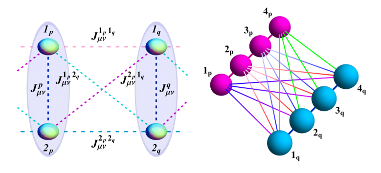
Figure 1: Schematic picture of the couplings between entangled pairs $p,q$ (left) and clusters (right) in Hamiltonian (8).

The ensuing internal equations $H_{p}|\psi_{p}\rangle=E_{p}|\psi_{p}\rangle$ are satisfied for a uniform field $\bm{b}^{1_{p}}=\bm{b}^{2_{p}}=\bm{b}^{p}$ at each pair and $J^{1_{p}2_{p}}_{\mu\nu}=J^{1_{p}2_{p}}_{\nu\mu}=\tfrac{1}{2}(J^{1_{p}1_{p}}_{\mu\nu}+J^{2_{p}2_{p}}_{\mu\nu})+J^{p}\delta_{\mu\nu}$ (App. D), such that for general $p,q$ and $s_{p}$, (9) is extended to

$${J}^{1_{p}2_{q}}_{\mu\nu}+{J}^{2_{p}1_{q}}_{\mu\nu}-{J}^{1_{p}1_{q}}_{\mu\nu}-{J}^{2_{p}2_{q}}_{\mu\nu}=2J^{p}\delta^{pq}\delta_{\mu\nu}\,,$$ (10)

implying $V_{pp}=J^{p}\bm{S}_{1_{p}}\cdot\bm{S}_{2_{p}}+\frac{1}{2}\sum_{i}J^{i_{p}i_{p}}_{\mu\nu}S_{i_{p}}^{\mu}S^{\nu}_{p}$ and $E_{p}=-J^{p}s_{p}(s_{p}+1)$. Eq.  (10) is the most general necessary and sufficient condition for exact singlet dimerization of an eigenstate under quadratic couplings, being GS if all $J_{p}>0$ are sufficient large.

Spin 0 clusters. We now consider products of general states $|\psi_{p}\rangle$ of $N_{p}\geq 3$ spins with $0$ total spin: $\bm{S}_{p}|\psi_{p}\rangle=\bm{0}$ for $\bm{S}_{p}=\sum_{j}\bm{S}_{j_{p}}$ ($N_{p}$ even if $s_{p}$ half-integer). Rotational invariance again implies $\langle\bm{S}_{i_{p}}\rangle=\bm{0}$ and $\langle S^{\mu}_{i_{p}}S^{\nu}_{j_{p}}\rangle=\delta^{\mu\nu}C_{i_{p}j_{p}}$ with $C_{i_{p}j_{p}}=\tfrac{1}{3}\langle\bm{S}_{i_{p}}\cdot\bm{S}_{j_{p}}\rangle$. Then (4b) leads to $C_{i_{p}k_{p}}C_{j_{q}l_{q}}{J}^{k_{p}l_{q}}_{\mu\nu}={0}$ $\forall\mu,\nu,p\neq q$, generalizing (9). However, as the $S_{p}^{\mu}$ are conserved, ${\bf C}_{p}\bm{n}^{\mu}=\bm{0}$ for $n^{\mu j_{p}}_{\nu}=\delta^{\mu}_{\nu}$. Then (6b) always yields a solution $J^{i_{p}j_{q}}_{\mu\nu}=K^{i_{p}q}_{\mu\nu}+K^{pj_{q}}_{\mu\nu}$, implying, $\forall\,i,j,k,l$, the sufficient conditions (App. E)

$${J}^{i_{p}j_{q}}_{\mu\nu}+{J}^{k_{p}l_{q}}_{\mu\nu}={J}^{i_{p}l_{q}}_{\mu\nu}+{J}^{k_{p}j_{q}}_{\mu\nu}\,,\;\;p\neq q,$$ (11)

which extend (9) and ensure again $V_{pq}|\Psi\rangle=0$, with $V_{pq}=K^{pj_{q}}_{\mu\nu}S^{\mu}_{p}S^{\nu}_{j_{q}}+K^{i_{p}q}_{\mu\nu}S^{\mu}_{i_{p}}S^{\nu}_{q}$. They are necessary if the $S^{\mu}_{p}$ are the only linear conserved operators.

Dividing each cluster in two halves $1^{\prime}_{p}$, $2^{\prime}_{p}$ of $\frac{1}{2}N_{p}$ spins, internal couplings fulfilling (10) applied to the spins $\bm{S}_{1^{\prime}_{p}}$ and $\bm{S}_{2^{\prime}_{p}}$ of each half lead to an $H_{p}$ having a unique GS $|\psi_{p}\rangle$ with $0$ total spin and maximum spin of each half, with ${S}_{p}^{\mu}$ the only linear conserved quantities (App. E).

States with null magnetization and generalized singlets. Consider now states with just null magnetization along $z$, $S^{z}_{p}|\psi_{p}\rangle=0$ for $S^{z}_{p}=\sum_{i}S^{z}_{i_{p}}$. Invariance under rotations around $z$ imply $\langle S^{\mu}_{i_{p}}\rangle=0$ for $\mu=x,y$ and $\langle\tilde{S}^{\mu{\dagger}}_{i_{p}}\tilde{S}^{\nu}_{j_{p}}\rangle=\delta^{\mu\nu}C^{\mu\mu}_{i_{p}j_{p}}$ for $\mu=\pm,z$ and $S^{\pm}_{i_{p}}=S^{x}_{i_{p}}\pm iS^{y}_{i_{p}}$, with $C^{--}_{i_{p}j_{p}}=\langle S^{+}_{i_{p}}S^{-}_{j_{p}}\rangle=C^{++}_{j_{p}i_{p}}+2\delta_{ij}\langle S^{z}_{i_{p}}\rangle$. Then Eq. (4b) implies

$$({\bf C}_{p}^{\mu\mu}\otimes{\bf C}_{q}^{\nu\nu}){\bm{J}}^{pq}_{\mu\nu}={\bf 0},\;\;\mu,\nu=\pm,z,$$ (12)

for ${\bf C}_{p}^{\mu\mu}$ matrices of elements $C^{\mu\mu}_{i_{p}j_{p}}$ and $\bm{J}^{pq}_{\mu\nu}$ vectors of components $J^{i_{p}j_{q}}_{\mu\nu}$ . Conservation of $S^{z}_{p}$ entails $C^{zz}_{p}$ singular, with (12) implying (11) for $\mu=\nu=z$ and $J^{i_{p}j_{q}}_{\mu z}=J_{\mu z}^{i_{p}k_{q}}$, $J^{i_{p}j_{q}}_{z\mu}=J_{z\mu}^{k_{p}j_{q}}$ for $\mu=\pm$, as sufficient conditions according to (6b). Further couplings are enabled if ${\bf C}_{p}^{\pm\pm}$ are also singular.

In the case of pairs, $|\psi_{p}\rangle=\sum_{m}\alpha_{m}|m,-m\rangle$. In order to have conserved operators $Q_{p}^{\pm}=a^{\pm}_{1}S^{\pm}_{1_{p}}+a^{\pm}_{2}S^{\pm}_{2_{p}}$ fulfilling (5), the only possibility is $\lambda^{\pm}_{p}=0$ and $\alpha_{m}/\alpha_{m+1}=-(a^{\pm}_{2}/a^{\pm}_{1})^{\pm 1}=\gamma$ constant, such that for $\gamma=-\tan\frac{\xi_{p}}{2}$,

$$|\psi_{p}\rangle\propto{\sum_{m=-s_{p}}^{s_{p}}}\!\!\!(\text{-}1)^{s_{p}\text{-}m}\!\cos^{s_{p}\text{+}m}\!\tfrac{\xi_{p}}{2}\sin^{s_{p}\text{-}m}\!\tfrac{\xi_{p}}{2}\left|m,-m\right\rangle.\;\;\;\;$$ (13)

These states (generalized singlets) are the only $S^{z}_{p}=0$ states with $3$ conserved linear operators: $Q_{p}^{\mu}|\psi_{p}\rangle=0$ for $\mu=z,\pm$, with $Q_{p}^{z}=S_{p}^{z}$, $Q_{p}^{+}=\cos\tfrac{\xi_{p}}{2}S_{1_{p}}^{+}\!+\!\sin\tfrac{\xi_{p}}{2}S_{2_{p}}^{+}$, $Q_{p}^{-}=\sin\tfrac{\xi_{p}}{2}S_{1_{p}}^{-}\!+\!\cos\tfrac{\xi_{p}}{2}S_{2_{p}}^{-}$. They satisfy $[Q_{p}^{+},Q_{p}^{-}]=\sin\xi_{p}Q^{z}_{p}$, $[Q_{p}^{z},Q_{p}^{\pm}]=\pm Q_{p}^{\pm}$. The standard, maximally entangled, singlet corresponds to $\xi_{p}=\frac{\pi}{2}$, where $Q_{p}^{\pm}\propto S_{p}^{\pm}$, while for $\xi_{p}\rightarrow 0,\pi$, $|\psi_{p}\rangle\rightarrow|\pm s,\mp s\rangle$ becomes separable. The reduced state of each spin in (13), $\rho_{i}={\rm tr}_{\bar{i}}\,|\psi_{p}\rangle\langle\psi_{p}|\propto e^{(-1)^{i}\beta S^{z}_{i_{p}}}$ for $\beta=\ln|\tan^{2}\frac{\xi_{p}}{2}|$, is exactly that of a spin $s_{p}$ paramagnet at temperature $T\propto\beta^{-1}$ (App. F).

For general $s_{p}$, the state (13) is, for instance, eigenstate of an $XXZ$ pair Hamiltonian in a nonuniform field,

$$H_{p}\! = \!b^{i_{p}}S^{z}_{i_{p}}\!+\!J^{p}(S^{x}_{1_{p}}S^{x}_{2_{p}}\!+\!S^{y}_{1_{p}}S^{y}_{2_{p}})\!+\!J^{p}_{z}S^{z}_{1_{p}}S^{z}_{2_{p}}\,\!,\;\;\;\;\;\;$$ (14)

if $\sin\xi_{p}=J^{p}/J^{p}_{z}$ and $b^{2_{p}}-b^{1_{p}}=J^{p}_{z}\cos\xi_{p}$, as then $H_{p}=\frac{b^{1_{p}}+b^{2_{p}}}{2}Q_{p}^{z}+\frac{1}{2}J_{z}^{p}\sum_{\mu=\pm,z}Q_{p}^{\mu{\dagger}}Q_{p}^{\mu}+E_{p}$,satisfying $H_{p}|\psi_{p}\rangle=E_{p}|\psi_{p}\rangle$ with $E_{p}=-s_{p}(s_{p}+1)J^{p}_{z}$. It is its GS if $J^{p}_{z}>0$ and $b^{1_{p}}=-b^{2_{p}}$ .

Previous coupling is just a special case of

$$V_{pq}=\tfrac{1}{2}(K^{pq}_{\mu\nu}Q^{\nu{\dagger}}_{q}Q^{\mu}_{p}+h.c.)+K^{pq}_{z-}S_{q_{-}}^{z}S_{p}^{z}\,,$$ (15)

where $\mu,\nu=\pm,z$ and $S^{z}_{q_{-}}=S^{z}_{1_{p}}-S^{z}_{2_{p}}$, which clearly satisfies $V_{pq}|\Psi\rangle=0\,\forall\,p,q$. It is the most general hermitian quadratic coupling compatible with generalized singlet factorization, and includes $XXZ$ ($K^{pq}_{\mu\nu}=\delta_{\mu\nu}J^{pq}_{\nu}$ real), $XYZ$ (previous case plus $K^{pq}_{\pm\mp}$ real) and DM-type ($K^{pq}_{\pm\pm}$ imaginary) couplings (App. F).

The state (13) leads to rank $1$ covariances ${\bf C}^{\mu\mu}_{p}\propto\bm{k}_{p}^{\mu}\bm{k}_{p}^{\mu{\dagger}}$ in (12), with $\bm{k}_{p}^{\mu{\dagger}}\bm{n}_{p}^{\mu}=0$ and $\bm{n}_{p}^{\mu}$ the nullspace vectors $\bm{n}^{+}_{p}=(\cos\frac{\xi_{p}}{2},\sin\frac{\xi_{p}}{2})$, $\bm{n}^{-}_{p}\!=\!(\sin\frac{\xi_{p}}{2},\cos\frac{\xi_{p}}{2})$ and $\bm{n}_{p}^{z}=(1,1)$ determining $Q_{p}^{\mu}$. The constraints (12) on $\bm{J}^{pq}_{\mu\nu}$ leading to the dimerizing coupling (15) have the form (10) for $\mu,\nu=\pm,z$ and $J^{i_{p}j_{q}}_{\mu\nu}\rightarrow J^{i_{p}j_{q}}_{\mu\nu}/(n^{\mu}_{i_{p}}n^{\nu}_{j_{q}})$, $\delta_{\mu\nu}\rightarrow\tilde{M}^{p}_{\mu\nu}$ (App. F). For $V_{pq}$ hermitian and $\xi_{p,q}\in\mathbb{R}$ they imply ($p\neq q$)

$$\sin\tfrac{\xi_{q}\pm\xi_{p}}{2}J^{D^{\pm}_{pq}}_{\mu\bar{\mu}} = \cos\tfrac{\xi_{q}\mp\xi_{p}}{2}J^{E^{\pm}_{pq}}_{\mu\bar{\mu}}\,,$$ (16a)

$$\cos\tfrac{\xi_{q}\mp\xi_{p}}{2}J^{D_{pq}^{\pm}}_{\mu\mu} = \sin\tfrac{\xi_{q}\pm\xi_{p}}{2}J^{E^{\pm}_{pq}}_{\mu\mu}\,,$$ (16b)

for $J^{D_{pq}^{\pm}}_{\mu\nu}=\frac{J^{1_{p}1_{q}}_{\mu\nu}\pm J^{2_{p}2_{q}}_{\mu\nu}}{2}$, $J^{E^{\pm}_{pq}}_{\mu\nu}=\frac{J^{1_{p}2_{q}}_{\mu\nu}\pm J^{2_{p}1_{q}}_{\mu\nu}}{2}$ and $\mu=\pm$, $\bar{\mu}=-\mu$, with $J^{D_{pq}^{+}}_{zz}=J^{E_{pq}^{+}}_{zz}$, entailing the constraints

$${J}^{D^{\pm}_{pq}}_{\mu\mu}{J}^{D^{\pm}_{pq}}_{\mu\bar{\mu}} = {J}^{E^{\pm}_{pq}}_{\mu\mu}{J}^{E^{\pm}_{pq}}_{\mu\bar{\mu}}\,.$$ (17)

Field induced dimerization in spin-$s$ XXZ systems. If $J^{i_{p}j_{q}}_{\pm\mp}=J^{i_{p}j_{q}}$, $J^{i_{p}j_{q}}_{\pm\pm}=0$ and $J^{i_{p}j_{q}}_{\mu,z}=\delta_{\mu z}J^{i_{p}j_{q}}_{z}$, we obtain $XXZ$-type couplings, where (16b)–(17) vanish and just (16a) remains. For a uniform dimerized eigenstate $\xi_{p}=\xi\,\forall\,p$, it implies $J^{1_{p}2_{q}}=J^{2_{p}1_{q}}=\frac{J^{1_{p}1_{q}}+J^{2_{p}2_{q}}}{2}\sin\xi$, whence $J^{i_{p}j_{q}}(S^{x}_{i_{p}}S^{x}_{j_{q}}+S^{y}_{i_{p}}S^{y}_{j_{q}})=\frac{1}{2}\sum_{\mu=\pm}J^{pq}_{\mu}(Q_{p}^{\mu{\dagger}}Q_{q}^{\mu}+h.c.)$ with $J^{pq}_{\pm}=J^{D^{+}_{pq}}\pm J^{D^{-}_{pq}}/\cos\xi$, of arbitrary range. For $H_{p}$ given by (14), such dimerized state will then emerge as exact GS at the local dimerizing field difference $b^{2_{p}}-b^{1_{p}}=J^{p}_{z}\cos\xi$ if $J^{p}_{z}>0$ is sufficiently large.

Example 1: MG model at finite field. For first neighbor couplings between pairs ($q=p+1$), with $J^{2_{p}1_{q}}=J^{E}$, $J^{1_{p}2_{q}}=0$, $J^{i_{p}i_{q}}=J^{D}$ (similarly for $J^{i_{p}j_{q}}_{zz}$), and $J^{p}=J$, $J^{p}_{z}=J_{z}$ in (14), the system becomes equivalent to a linear chain with first-and second-neighbor couplings (Fig. 2 top), with the original isotropic MG model recovered for $J^{E}=2J^{D}=J$ and zero field.

Then, for general $J^{D},J^{E}$ Eq. (16a) implies an exact alternating dimerized eigenstate with $\xi_{p}=\pi-\xi_{q}=\xi$ and $\sin\xi=2J^{D}/J^{E}$ if $2|J^{D}|\leq|J^{E}|$ and $J_{z}^{E}=2J^{D}_{z}$, at an alternating field $b^{2_{p}}-b^{1_{p}}=(-1)^{p+1}J_{z}\cos\xi$, with $J_{z}=\frac{1}{2}JJ^{E}/J^{D}$ if $s_{p}=s\geq 1$ Note (3). It will be GS for large $J_{z}>0$, with $J\geq J^{E}$ sufficient if $s=1/2$ (see plots in App. G). The degeneracy of the dimerized GS in the MG case $\xi=\pi/2$ due to translational invariance in the cyclic chain with $J=J^{E}$ is broken for $|J^{E}|>2|J^{D}|$ since the dimerizing field is nonuniform.

Field induced dimerization in $XYZ$ systems. Through a local rotation $|\psi_{p}\rangle\rightarrow|\psi_{p}^{+}\rangle=e^{-i\pi S^{x}_{2_{p}}}|\psi_{p}\rangle$ in (13) ($|m,-m\rangle\rightarrow|m,m\rangle$), the generalized singlet becomes suitable for dimerization in anisotropic $XYZ$ systems, where $H_{p}=b^{i_{p}}S^{z}_{i_{p}}+\sum_{\mu}J^{p}_{\mu}S^{\mu}_{1_{p}}S^{\mu}_{2_{p}}$ and $J^{i_{p}j_{q}}_{\mu\nu}=J^{i_{p}j_{q}}_{\mu}\delta_{\mu\nu}$ ($\mu=x,y,z$). Setting $|\psi_{p}^{-}\rangle=|\psi_{p}\rangle$, the dimerizing conditions for a general product $\otimes_{p}|\psi_{p}^{\sigma_{p}}\rangle$ ($\sigma_{p}=\pm 1$) are obtained replacing ${J}^{i_{p}j_{q}}_{\mu}\rightarrow(-\sigma_{p})^{i_{p}-1}(-\sigma_{q})^{j_{q}-1}J^{i_{p}j_{q}}_{\mu}$ for $\mu=y,z$ in previous equations. If $s_{p}=1/2$,

$$|\psi_{p}^{\pm}\rangle = \cos\tfrac{\xi^{\pm}_{p}}{2}|\tfrac{1}{2},\pm\tfrac{1}{2}\rangle-\sin\tfrac{\xi^{\pm}_{p}}{2}|-\!\tfrac{1}{2},\mp\tfrac{1}{2}\rangle,$$ (18)

are just the eigenstates of previous $H_{p}$ for $b^{2_{p}}\pm b^{1_{p}}=\tfrac{1}{2}(J^{p}_{y}\mp J^{p}_{x})\cot\xi_{p}^{\pm}$, with energies $E_{p}^{\pm}=-\frac{1}{4}(\Delta_{p}^{\pm}\!\mp\!J_{z}^{p})$ ($\Delta_{p}^{\pm}=\frac{J^{p}_{x}\mp J^{p}_{y}}{\sin\xi_{p}^{\pm}}$), entailing a $|\psi_{p}^{+}\rangle\to|\psi_{p}^{-}\rangle$ GS transition at $J^{p}_{z}=\frac{\Delta_{p}^{+}-\Delta_{p}^{-}}{2}$ . If $J^{i_{p}i_{q}}_{\mu}=r_{pq}J^{D}_{\mu}$, $J^{1_{p}2_{q}}_{\mu}=J^{2_{p}1_{q}}_{\mu}=r_{pq}J^{E}_{\mu}$, (Fig. 2), uniform dimerized eigenstates $|\Psi^{\pm}\rangle=\otimes_{p}|\psi_{p}^{\pm}\rangle$ with $\xi_{p}^{\pm}=\xi^{\pm}$, $\sin\xi^{\pm}=J^{E}_{\mp}/J^{D}_{+}$ ($J^{\alpha}_{\pm}=J^{\alpha}_{x}\pm J^{\alpha}_{y}$) arise at previous fields if $|J^{E}_{\pm}|\leq|J^{D}_{+}|$ and $J^{D}_{z}=\mp J^{E}_{z}$, $J^{D}_{+}J^{D}_{-}=J^{E}_{+}J^{E}_{-}$ (Eqs. (16)–(17)), with $E=\sum_{p}E^{\pm}_{p}$. They are GS if $J_{z}^{p}{\genfrac{}{}{0.0pt}{2}{<}{>}}0$ is sufficiently large (App. G).

Example 2: Controlled dimerization with $XYZ$ couplings. For $4$ spins $1/2$ with $J^{p}_{\mu}=J_{\mu}$, $J^{E}_{x,y}=J_{x,y}$, $J^{E,D}_{z}=0$, we obtain the scheme of Fig. 2 (bottom): “vertical” uniform dimerized states $|\Psi^{\pm}\rangle$ are simultaneous eigenstates of $H$ at fields $b^{i_{p}}=B_{i}$ fulfilling previous conditions, with energies $E^{\pm}=-\frac{1}{2}(J^{D}_{+}\mp J_{z})$ and $|\psi^{\pm}\rangle$ GS for $J_{z}\,\genfrac{}{}{0.0pt}{2}{<}{>}J_{z}^{c\pm}$ if $J^{D}_{+}>0$. Remarkably, an “horizontal” mixed parity dimerized state $|\psi^{\prime+}_{1_{p}1_{q}}\rangle|\psi^{\prime-}_{2_{p}2_{q}}\rangle$ is also eigenstate of the same $H$ according to (16)-(17), with $\tan\xi^{\prime+}=-\frac{1}{4}J^{D}_{-}/B_{1}$, $\xi^{\prime-}=\frac{\pi}{2}$ and $E^{\prime}=-\frac{1}{2}(J^{D}_{+}+\Delta)$, becoming GS in the intermediate sector $J_{z}^{c+}<J_{z}<J_{z}^{c-}$, with $J_{z}^{c\pm}=\mp\sqrt{{J_{x}^{D}}^{\,2}-J_{x}^{2}}$. Hence type and geometry of the GS dimerization can be selected with $J_{z}$. The outer dimerized phases remain GS in larger systems (App. G).

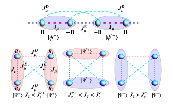
Figure 2: Top: Dimerization in the linear $XXZ$ chain for nonuniform field. Bottom: Schematic picture of the dimerized GSs of a $4$-spin $XYZ$ system for increasing $J_{z}$ at fixed upper and lower fields $B_{1},B_{2}$. Here $|\Psi^{\pm}\rangle$, $|\Psi^{\prime\pm}\rangle$ are entangled “vertical” and “horizontal” pair states of the form (18).

In summary, the present method can rapidly provide the pertinent constraints on fields and couplings for exact eigenstate factorization, requiring just local averages. It highlights the key role of local conserved operators obtained from its nullspace, allowing direct construction of compatible couplings and Hamiltonians. The possibility of a systematic exploration of interacting Hamiltonians having cluster-type factorized eigenstates at critical separability points is then opened up. Extensions to more general couplings and systems are under investigation.

SUPPLEMENTAL MATERIAL

Appendix A Quantum covariance matrix

Given a set of linearly independent operators $S^{\mu}$, we define the quantum covariance matrix ${\bf C}$ of elements

$$C^{\mu\nu}=\langle\tilde{S}^{\mu{\dagger}}\tilde{S}^{\nu}\rangle=\langle S^{\mu{\dagger}}S^{\nu}\rangle-\langle S^{\mu{\dagger}}\rangle\langle S^{\nu}\rangle\,,$$ (19)

where $\tilde{S}^{\mu}=S^{\mu}-\langle S^{\mu}\rangle$ and the averages are taken with respect to a general quantum density operator $\rho$ (positive semidefinite with unit trace): $\langle O\rangle={\rm Tr}\,(\rho\,O)$.

${\bf C}$ is an hermitian positive semidefinite matrix: It can be diagonalized by operators $O^{\mu}={U}^{\mu}_{\nu}S^{\nu}$ satisfying

$$\langle{\tilde{O}}^{\mu{\dagger}}{\tilde{O}}^{\nu}\rangle = \langle O^{\mu{\dagger}}O^{\nu}\rangle-\langle O^{\mu{\dagger}}\rangle\langle O^{\nu}\rangle=U^{\mu*}_{\mu^{\prime}}C^{\mu^{\prime}\nu^{\prime}}U^{\nu}_{\nu^{\prime}}\;\;\;\;\;\;$$ (20)

$$= \bm{U}^{\mu{\dagger}}{\bf C}\bm{U}^{\nu}=\delta^{\mu\nu}c^{\mu}\geq 0\,,\;\;\;\;\;\;$$ (21)

if $U^{\mu}_{\nu}$ are the elements of a unitary matrix diagonalizing ${\bf C}$, where $c^{\mu}=\langle{\tilde{O}}^{\mu{\dagger}}{\tilde{O}}^{\mu}\rangle\geq 0$ since ${\tilde{O}}^{\mu{\dagger}}{\tilde{O}}^{\mu}$ is always an hermitian positive semidefinite operator.

Therefore ${\rm det}\,{\bf C}=0$ iff $c^{\mu}=\langle\tilde{O}^{\mu{\dagger}}\tilde{O}^{\mu}\rangle=0$ for some $\mu$, i.e. iff there is a linear combination $O^{\mu}=U^{\mu}_{\nu}S^{\nu}\neq 0$ of the original operators with zero covariance with its adjoint. In such a case the associated eigenvector $\bm{U}^{\mu}$ belongs to the nullspace of ${\bf C}$: ${\bf C}\bm{U}^{\mu}=\bm{0}$.

For a pure $\rho=|\psi\rangle\langle\psi|$, $\langle O^{\mu}\rangle=\langle\psi|O^{\mu}|\psi\rangle$. Hence $\langle\tilde{O}^{\mu{\dagger}}\tilde{O}^{\mu}\rangle=\langle\psi|\tilde{O}^{\mu{\dagger}}\tilde{O}^{\mu}|\psi\rangle=0$ iff $\tilde{O}^{\mu}|\psi\rangle=0$, i.e. iff $O^{\mu}|\psi\rangle=\langle O^{\mu}\rangle|\psi\rangle$, such that $|\psi\rangle$ is an eigenstate of $O^{\mu}$:

$$\langle\psi|\tilde{O}^{\mu{\dagger}}\tilde{O}^{\mu}|\psi\rangle=0\;\;\iff\;\;\;O^{\mu}|\psi\rangle=\lambda^{\mu}|\psi\rangle,$$ (22)

with $\langle\psi|O^{\mu}|\psi\rangle=\lambda^{\mu}$ and $\tilde{O}^{\mu}=O^{\mu}-\lambda^{\mu}$. Thus, in the pure case ${\rm det}\,{\bf C}\,=0$ iff $|\psi\rangle$ is an eigenstate of a linear combination $O^{\mu}=U^{\mu}_{\nu}S^{\nu}\neq 0$ of the operators $S^{\mu}$ determining $C$, i.e. iff there is a “conserved” (in the sense of non-fluctuating) $O^{\mu}$. The set of conserved operators linear in the $S^{\nu}$ is determined by the nullspace of ${\bf C}$.

If $|\psi\rangle$ belongs to a Hilbert space ${\cal H}$ of finite dimension $D={\rm dim}\,{\cal H}$, and $\{|m\rangle,m=0,\ldots,D-1\}$ is an orthogonal ($\langle m|m^{\prime}\rangle=\delta_{mm^{\prime}}$) basis of ${\cal H}$ with $|0\rangle=|\psi\rangle$, ${\bf C}$ is diagonal for the basic operators $O^{mn}=|m\rangle\langle n|$:

$$\langle\tilde{O}^{mn{\dagger}}\tilde{O}^{m^{\prime}n^{\prime}}\rangle=\delta^{mm^{\prime}}\delta^{nn^{\prime}}\delta^{n0}(1-\delta^{m0})$$ (23)

entailing ${\rm rank}\,{\bf C}=D-1$ for a complete set of operators $S^{\mu}$ and ${\rm rank}\,{\bf C}\leq D-1$ for an arbitrary reduced set, always for averages determined by a pure state $|\psi\rangle$. Then ${\bf C}$ is always singular if the size $d$ of ${\bf C}$, i.e. the number of (linearly independent) operators $S^{\mu}$, satisfies $d\geq D$.

For averages with respect to mixed states $\rho=\sum_{\alpha}p_{\alpha}|\psi_{\alpha}\rangle\langle\psi_{\alpha}|$ ($p_{\alpha}>0$), $\langle\tilde{O}^{\mu{\dagger}}\tilde{O}^{\mu}\rangle=\sum_{\alpha}p_{\alpha}\langle\tilde{O}^{\mu{\dagger}}\tilde{O}^{\mu}\rangle_{\alpha}=0$ iff $\langle\tilde{O}^{\mu{\dagger}}\tilde{O}^{\mu}\rangle_{\alpha}=\langle\psi_{\alpha}|\tilde{O}^{\mu{\dagger}}\tilde{O}^{\mu}|\psi_{\alpha}\rangle=0$ $\forall$ $\alpha$, implying that all $|\psi_{\alpha}\rangle$ should be eigenstates of $O^{\mu}$ with the same eigenvalue. The rank of ${\bf C}$ can now be larger, having maximum rank $D^{2}-1$ for a complete set of $S^{\mu}$ if $\rho$ has maximum rank $D$: In this case $O|\psi_{\alpha}\rangle=\lambda|\psi_{\alpha}\rangle$ $\forall$ $\alpha$ implies $O=\lambda\mathbbm{1}$, such that the identity will be the sole operator with zero covariance. Thus, maximum rank of $\rho$ implies no local conserved operators (except for the identity).

For a general hermitian Hamiltonian $H=\sum_{\mu}J_{\mu}S^{\mu}$, with $S^{\mu}$ arbitrary many body operators, Eq. (22) shows that a general state $|\Psi\rangle$ is an eigenstate of $H$ iff

$$\langle\Psi|\tilde{H}^{2}|\Psi\rangle={\bf J}^{\dagger}C{\bf J}=0$$ (24)

for $\tilde{H}=H-\langle H\rangle$ and ${\bf C}$ a covariance matrix of elements (19) for these general $S^{\mu}$, with $\langle\ldots\rangle=\langle\Psi|\ldots|\Psi\rangle$. And since for a positive semidefinite ${\bf C}$, $\bm{J}^{\dagger}{\bf C}\bm{J}=||\sqrt{\bf C}\bm{J}||^{2}$, Eq. (24) is equivalent to $\sqrt{\bf C}\bm{J}=\bm{0}$, and hence to

$${\bf C}\bm{J}=\bm{0}\,.$$ (25)

Therefore, $|\Psi\rangle$ is eigenstate of $H$ iff (25) holds.

In the case of the product eigenstate (1) and Hamiltonian (2), Eq. (25) is equivalent to Eqs. (4), as we now show. It is first seen that

$$\langle\tilde{S}_{p}^{\mu}\tilde{S}_{q}^{\nu}\rangle = \delta_{pq}C_{p}^{\mu\nu}$$ (26)

with $C_{p}^{\mu\nu}$ now a local covariance matrix determined by the local state $|\psi_{p}\rangle$ of elements (19) for $S^{\mu}=S_{p}^{\mu}$, since for $p\neq q$, $\langle O_{p}Q_{q}\rangle=\langle O_{p}\rangle\langle O_{q}\rangle$ for averages with respect to a product state $|\Psi_{pq}\rangle=|\psi_{p}\rangle|\psi_{q}\rangle$, and hence $\langle\tilde{O}_{p}\tilde{O}_{q}\rangle=\langle\tilde{O}_{p}\rangle\langle\tilde{O}_{q}\rangle=0$ if $\tilde{O}_{p}=O_{p}-\langle O_{p}\rangle$. Similarly, for $q\neq q^{\prime}$,

$$\langle\tilde{S}_{p}^{\mu}\tilde{S}_{q}^{\nu}\tilde{S}_{q^{\prime}}^{\nu^{\prime}}\rangle=\delta_{pq}C_{p}^{\mu\nu}\langle\tilde{S}^{\nu^{\prime}}_{q^{\prime}}\rangle+\delta_{pq^{\prime}}C_{p}^{\mu\nu^{\prime}}\langle\tilde{S}_{q}\rangle=0$$ (27)

for any $p$, since $\langle\tilde{S}_{q}\rangle=\langle\tilde{S}_{q}\rangle=0$. Finally, if $p\neq q$, $p^{\prime}\neq q^{\prime}$,

$$\langle\tilde{S}_{p}^{\mu}\tilde{S}_{q}^{\nu}\tilde{S}_{p^{\prime}}^{\mu^{\prime}}\tilde{S}_{q^{\prime}}^{\nu^{\prime}}\rangle = \delta_{pp^{\prime}}\delta_{qq^{\prime}}C_{p}^{\mu\mu^{\prime}}\!C_{q}^{\nu\nu^{\prime}}\!\!\!+\delta_{pq^{\prime}}\delta_{qp^{\prime}}C_{p}^{\mu\nu^{\prime}}C_{q}^{\nu\mu^{\prime}}\!,\;\;\;\;\;\;\;\;\;$$ (28)

as $\langle\tilde{S}_{p}^{\mu}\tilde{S}_{q}^{\nu}\tilde{S}_{p}^{\mu^{\prime}}\tilde{S}_{q}^{\nu^{\prime}}\rangle=\langle\tilde{S}_{p}^{\mu}\tilde{S}_{p}^{\mu^{\prime}}\rangle\langle\tilde{S}_{q}^{\nu}\tilde{S}_{q}^{\nu^{\prime}}\rangle$, i.e.  ${\bf C}_{pq}={\bf C}_{p}\otimes{\bf C}_{q}$ for a product state $|\Psi_{pq}\rangle=|\psi_{p}\rangle|\psi_{q}\rangle$.

Hence, the full covariance matrix ${\bf C}$ in (26) becomes split in local blocks ${\bf C}_{p}$ associated to the one-body terms $\bm{h}^{p}\cdot\bm{S}_{p}$ and blocks ${\bf C}_{p}\otimes{\bf C}_{q}$ associated to the residual two-body terms in Eq. (2b), such that Eq. (25) becomes equivalent to Eqs. (4).

Numerical methods for Hamiltonian construction from a given general eigenstate, based on a global covariance matrix, were recently introduced in Chertkov and Clark (2018); Qi and Ranard (2019). Related quantum covariance matrices were used previously in connection with the detection of entanglement Gühne et al. (2007). See also Gordon et al. (2022); Boyd and Koczor (2022) for other recent uses of covariance based quantum formalisms.

Appendix B Full factorization in spin systems

For a general spin array in a magnetic field, full standard factorization corresponds to a product eigenstate $|\Psi\rangle=\otimes_{p}|\bm{n}_{p}\rangle$ with maximum spin at each site along a general local direction

$$\bm{n}_{p}=\left(\sin\theta_{p}\cos\phi_{p},\sin\theta_{p}\sin\phi_{p},\cos\theta_{p}\right)\equiv\bm{n}_{p}^{z^{\prime}}\,,$$ (29)

such that $\bm{n}_{p}\cdot\bm{S}_{p}|\bm{n}_{p}\rangle=s_{p}|\bm{n}_{p}\rangle$ Kurmann et al. (1982); Müller and Shrock (1985); Roscilde et al. (2004); Amico et al. (2006); Giampaolo et al. (2008); Rossignoli et al. (2008, 2009); Giorgi (2009); Giampaolo et al. (2009); Abouie et al. (2012); Cerezo et al. (2015, 2017); Yi et al. (2019); Thakur and Durganandini (2020); Canosa et al. (2020); Su et al. (2022); Chitov et al. (2022). We derive here the associated factorizing conditions with the covariance method.

Since $D_{p}={\rm dim}{\cal H}_{p}=2$ for $s_{p}=1/2$, the $3\times 3$ covariance matrix ${\bf C}_{p}$ of the three local spin operators $S_{p}^{\mu}$ will have rank $D_{p}-1=1$. The same holds for arbitrary spin $s_{p}$ since for such state the covariance matrix will be proportional to that for $s_{p}=1/2$. Hence it will be singular, enabling non-trivial factorization.

If $\bm{n}_{p}=\bm{n}_{z}=(0,0,1)$ ($\theta_{p}=0$), $\langle S^{\mu}_{p}\rangle=s_{p}\delta^{\mu z}$ and

$${\bf C}_{p}^{\mu\nu}=\langle S_{p}^{\mu}S_{p}^{\nu}\rangle-\langle S_{p}^{\mu}\rangle\langle S_{p}^{\nu}\rangle=\frac{1}{2}s_{p}[\delta^{\mu\nu}(1-\delta^{\mu z})+i\epsilon^{\mu\nu z}]\,,$$

with $\epsilon$ the fully antisymmetric tensor, such that

$${\bf C}_{p} = \tfrac{1}{2}s_{p}\begin{pmatrix}\,\,1&i&0\\ -i&1&0\\ \,\,0&0&0\end{pmatrix}=\tfrac{1}{2}s_{p}\begin{pmatrix}\,\,1\\ -i\\ \,\,0\end{pmatrix}\begin{pmatrix}1&i&0\end{pmatrix}$$ (30)

$$= \tfrac{1}{2}s_{p}\bm{n}^{-}\bm{n}^{-{\dagger}}\,,$$ (31)

where $\bm{n}^{\pm}=\bm{n}^{x}\pm i\bm{n}^{y}$. The result for a general $\bm{n}_{p}$ then follows by rotation:

$${\bf C}_{p}=\tfrac{1}{2}s_{p}\bm{n}_{p}^{-}\bm{n}_{p}^{-\dagger}\,,$$ (32)

where $\bm{n}_{p}^{\pm}=\bm{n}_{p}^{x^{\prime}}\pm\imath\bm{n}_{p}^{y^{\prime}}$ (with $\bm{k}_{p}=\bm{n}_{p}^{-}$ in main text) and

$$\bm{n}_{p}^{x^{\prime}} = (\cos\theta_{p}\cos\phi_{p},\cos\theta_{p}\sin\phi_{p},-\sin\theta_{p})\,,$$ (33a)

$$\bm{n}_{p}^{y^{\prime}} = (-\sin\phi_{p},\cos\phi_{p},0)\,,$$ (33b)

are rotated unit vectors orthogonal to $\bm{n}_{p}^{z^{\prime}}$. In matrix Eqs.  like (31)-(32), $\bm{n}_{p}^{\mu}$ ($\bm{n}_{p}^{\mu{\dagger}}$) stand for column (row) vectors.

The matrix (32) is then verified to have rank $1$, having a single nonzero eigenvalue $s_{p}$ with eigenvector $\bm{n}_{p}^{-}$: ${\bf C}_{p}\bm{n}_{p}^{-}=s_{p}\bm{n}_{p}^{-}$. Its nullspace is then spanned by the orthogonal vectors $\bm{n}_{p}$ and $\bm{n}_{p}^{+}$: ${\bf C}_{p}\bm{n}_{p}={\bf C}_{p}\bm{n}_{p}^{+}=\bm{0}$, which generate the two local conserved operators $Q_{p}^{z^{\prime}}=\bm{n}_{p}\cdot\bm{S}_{p}=S_{p}^{z^{\prime}}$, $Q_{p}^{+^{\prime}}=\bm{n}_{p}^{+}\cdot\bm{S}_{p}=S_{p}^{+^{\prime}}=S_{p}^{x^{\prime}}+iS_{p}^{+^{\prime}}$, satisfying

$$S_{p}^{z^{\prime}}|\bm{n}_{p}\rangle=s_{p}|\bm{n}_{p}\rangle,\;\;S_{p}^{+^{\prime}}|\bm{n}_{p}\rangle=0\,.$$ (34)

This enables full factorization with nontrivial couplings.

Using (32), Eqs. (4) lead at once to the two complex equations

$$\bm{n}_{p}^{-{\dagger}}\bm{h}^{p} = 0\,,$$ (35a)

$$(\bm{n}_{p}^{-{\dagger}}\otimes\bm{n}_{q}^{-{\dagger}})\bm{J}^{pq} = 0\,,$$ (35b)

where $\bm{h}^{p}=\bm{b}^{p}+\sum\limits_{q\neq p}s_{q}{\bf J}^{pq}\bm{n}_{q}$ and $\bm{J}^{pq}$ is a vector of components $J^{pq}_{\mu\nu}$. They can be rewritten as

$$(\bm{n}_{p}^{x^{\prime}}+i\bm{n}_{p}^{y^{\prime}})\cdot{\bm{h}}^{p} = 0\,,$$ (36a)

$$(\bm{n}_{p}^{x^{\prime}}+i\bm{n}_{p}^{y^{\prime}})\cdot{\bf J}^{pq}(\bm{n}_{q}^{x^{\prime}}+i\bm{n}_{q}^{y^{\prime}}) = 0\,.$$ (36b)

where ${\bf J}^{pq}$ is a matrix of elements $J^{pq}_{\mu\nu}$. For real fields and couplings ($H$ hermitian) they lead to

$$\bm{n}_{p}^{x^{\prime}}\cdot{\bm{h}}^{p}=0\,,\;\;\;\;\bm{n}_{p}^{y^{\prime}}\cdot{\bm{h}}^{p} = 0\,,$$ (37a)

$$\bm{n}_{p}^{x^{\prime}}\cdot{\bf J}^{pq}\bm{n}_{q}^{x^{\prime}}-\bm{n}_{p}^{y^{\prime}}\cdot{\bf J}^{pq}\bm{n}_{q}^{y^{\prime}} = 0\,,$$ (37b)

$$\bm{n}_{p}^{x^{\prime}}\cdot{\bf J}^{pq}\bm{n}_{q}^{y^{\prime}}+\bm{n}_{p}^{y^{\prime}}\cdot{\bf J}^{pq}\bm{n}_{q}^{x^{\prime}} = 0\,,$$ (37c)

thus coinciding with the general factorization equations of Ref. Cerezo et al. (2015). Eqs. (37a) determine the factorizing fields, implying ${\bm{h}}^{p}$ parallel to $\bm{n}_{p}$ ($\bm{n}_{p}\times{\bm{h}}^{p}=\bm{0}$) whereas (37b)–(37c) are the explicit linear constraints on the coupling strengths, entailing that all terms $\propto S_{p}^{-^{\prime}}S_{q}^{-^{\prime}}$ in the $p-q$ coupling should vanish.

With these constrains, the Hamiltonian has the form

$$H = \sum_{p}e^{p}S_{p}^{z^{\prime}}+\tfrac{1}{2}\sum_{p\neq q}K^{pq}_{\alpha\beta}\tilde{S}_{p}^{\alpha{\dagger}}\tilde{S}_{q}^{\beta}$$ (38a)

$$= \tfrac{1}{2}\sum_{p,q}K^{pq}_{\alpha\beta}\tilde{S}_{q}^{\beta\dagger}\tilde{S}_{p}^{\alpha}+E$$ (38b)

with $\alpha,\beta=z^{\prime},+^{\prime}$, $K^{pp}_{\alpha\beta}=-2e^{p}/(2s_{p}+1)\delta_{\alpha\beta}$ and $E=\sum_{p}e^{p}s_{p}$. Then, if the whole matrix $K^{pq}_{\alpha\beta}$ (with $p=q$ terms included) is positive definite, $|\Psi\rangle$ will be GS of $H$. This is obviously ensured by a sufficiently large $e^{p}<0$.

Appendix C General internal equations

We consider now a Hamiltonian with internal quadratic terms, such that the internal Hamiltonian becomes

$$H_{p}=\bm{b}^{p}\cdot\bm{S}_{p}+\tfrac{1}{2}\bm{S}_{p}\cdot{\bf J}^{pp}\bm{S}_{p}.$$ (39)

Eq. (4b) remains unaltered for the coupling between sites, implying (6b), but Eq. (4a) now requires in principle an enlarged covariance matrix including operators quadratic in the $S_{p}^{\mu}$. Nonetheless, the existence of “linear” conserved quantities $Q_{p}^{\alpha}=n_{p\mu}^{\alpha}S_{p}^{\mu}$ provides a particular solution of the ensuing Eq. (4a). Assuming a closed algebra $[S^{\mu}_{p},S^{\nu}_{q}]=\delta_{pq}f^{\mu\nu}_{p\mu^{\prime}}S^{\mu^{\prime}}_{p}$ and hence a symmetric coupling $J^{pp}_{\mu\nu}=J^{pp}_{\nu\mu}$ to avoid linear terms already covered by the field term, a solution of the internal equations is

$$\bm{h}^{p} = h^{p}_{\alpha}\bm{n}^{\alpha}_{p}-\Delta\bm{h}^{p}\,,$$ (40a)

$${\bm{J}}^{pp} = {\bm{n}}_{p}^{\alpha}\otimes{\bm{K}}^{p}_{\alpha}+\bm{K}^{p}_{\;\alpha}\otimes\bm{n}_{p}^{\alpha}\,,$$ (40b)

where $\bm{h}^{p}=\bm{b}^{p}+\sum_{q}{\bf J}^{pq}\langle\bm{S}_{q}\rangle$ and $\Delta{h}^{p}_{\mu}=\tfrac{1}{2}f^{\mu^{\prime}\nu^{\prime}}_{p\mu}n_{p\mu^{\prime}}^{\alpha}K^{p}_{\alpha\nu^{\prime}}$, such that

$$\Delta\bm{h}^{p}\cdot\bm{S}_{p}=\tfrac{1}{2}[Q_{p}^{\alpha},\bm{K}^{p}_{\alpha}\cdot\bm{S}_{p}]\,.$$ (41)

In this way, $\bm{h}^{p}\cdot\bm{S}_{p}=h^{p}_{\alpha}Q_{p}^{\alpha}-\tfrac{1}{2}[Q_{p}^{\alpha},\bm{K}^{p}_{\alpha}\cdot\bm{S}_{p}]$ and $V_{pp}=2\bm{S}_{p}\cdot\bm{K}^{p}_{\alpha}Q_{p}^{\alpha}+[Q_{p}^{\alpha},\bm{K}^{p}_{\alpha}\cdot\bm{S}_{p}]$, the last commutator cancelled by the previous term in $\bm{h}^{p}\cdot\bm{S}_{p}$. This is feasible provided $[Q_{p}^{\alpha},\bm{K}^{p}_{\alpha}\cdot\bm{S}_{p}]$ vanishes or is hermitian, and leads to a final internal Hamiltonian $H_{p}={\bm{b}^{\prime}}^{p}\cdot\bm{S}_{p}+\bm{S}_{p}\cdot\bm{K}^{p}_{\alpha}Q_{p}^{\alpha}$, with ${\bm{b}^{\prime}}^{p}=\bm{b}^{p}-\Delta\bm{h}^{p}$. The operator $\bm{K}^{p}\cdot\bm{S}_{p}$ is in principle arbitrary (complying with the hermiticity of $H_{p}$) and in particular, includes the possibility of generating a positive semidefinite form $\frac{1}{2}K^{pp}_{\alpha\beta}Q^{\beta{\dagger}}_{p}Q_{p}^{\alpha}$.

Eqs. (40) are equivalent to

$${\bf C}_{p}(\bm{h}^{p}+\Delta\bm{h}^{p}) = 0,$$ (42a)

$$({\bf C}_{p}\otimes{\bf C}_{p}){\bm{J}}^{pp} = 0\,.$$ (42b)

which constitute a generalization (for $q=p$) of Eqs. (4).

If $|\psi_{p}\rangle$ has extra (quadratic) conserved quantities of the form $Q_{p}=h^{\prime p}_{\mu}S_{p}^{\mu}+J^{\prime pp}_{\mu\nu}S_{p}^{\mu}S_{p}^{\nu}$, like e.g. quadratic Casimir operators, then Eq. (42) holds for $h^{p}_{\mu}\rightarrow h^{p}_{\mu}+h^{\prime p}_{\mu}$ and $J^{pp}_{\mu\nu}\rightarrow J^{pp}_{\mu\nu}+J^{\prime pp}_{\mu\nu}$.

Appendix D Spin zero pairs

D.1 Factorizing equations

For a spin pair coupled to $0$ total spin, the cluster state is given by the standard singlet (Eq. (13)) for $\xi_{p}=\pi/2$), satisfying

$$\bm{S}_{p}|\psi_{p}\rangle=\bm{0}\,,\;\;\bm{S}_{p}=\bm{S}_{1_{p}}+\bm{S}_{2_{p}}=\bm{Q}_{p}\,.$$ (43)

Then the elements of the ensuing covariance matrix ${\bf C}_{p}$ of the spin operators $S^{\mu}_{i_{p}}$ become ($i,j=1,2$)

$$C_{i_{p}j_{p}}^{\mu\nu} = \langle S^{\mu}_{i_{p}}S^{\nu}_{j_{q}}\rangle-\langle S^{\mu}_{i_{p}}\rangle\langle S^{\nu}_{j_{q}}\rangle$$ (44)

$$= \tfrac{1}{3}\langle{\bm{S}_{i_{p}}}\cdot{\bm{S}_{j_{p}}}\rangle\delta^{\mu\nu}=\kappa_{p}(-1)^{i-j}\delta^{\mu\nu},$$

for $\kappa_{p}=\frac{s_{p}(s_{p}+1)}{3}$, such that $\forall$ $p$, ${\bf C}_{p}$ is the $6\times 6$ matrix

$${\bf C}_{p}=\kappa_{p}\begin{pmatrix}\;\;\mathbbm{1}&-\mathbbm{1}\\ -\mathbbm{1}&\;\;\mathbbm{1}\end{pmatrix}=\kappa_{p}\sum_{\mu}\,\bm{k}^{\mu}\bm{k}^{\mu{\dagger}}\,,$$ (45)

where $k^{\mu}_{i_{p}\nu}=(-1)^{i_{p}}\delta^{\mu}_{\nu}$. Hence for $p\neq q$ Eqs. (4b) become

$$({\bf C}_{p}\otimes{\bf C}_{q})\bm{J}^{pq} = \kappa_{p}\kappa_{q}\begin{pmatrix}\;\;\mathbbm{1}&-\mathbbm{1}&-\mathbbm{1}&\;\;\mathbbm{1}\\ -\mathbbm{1}&\;\;\mathbbm{1}&\;\;\mathbbm{1}&-\mathbbm{1}\\ -\mathbbm{1}&\;\;\mathbbm{1}&\;\;\mathbbm{1}&-\mathbbm{1}\\ \;\;\mathbbm{1}&-\mathbbm{1}&-\mathbbm{1}&\;\;\mathbbm{1}\end{pmatrix}\begin{pmatrix}{\bm{J}}^{1_{p}1_{q}}\\ {\bm{J}}^{1_{p}2_{q}}\\ {\bm{J}}^{2_{p}1_{q}}\\ {\bm{J}}^{2_{p}2_{q}}\end{pmatrix}=\bm{0}$$

where ${\bm{J}}^{i_{p}j_{q}}$ are vectors of components $J^{i_{p}j_{q}}_{\mu\nu}$, implying

$${\bm{J}}^{1_{p}1_{q}}-{\bm{J}}^{1_{p}2_{q}}-{\bm{J}}^{2_{p}1_{q}}+{\bm{J}}^{2_{p}2_{q}}=0,$$ (46)

i.e., Eq. (9). Since ${\bf C}_{p}$, has rank $3$ $\forall\,p$, ${\bf C}_{p}\otimes{\bf C}_{q}$ has rank $9$, then leading to the $9$ constraints (46) on the couplings $J^{i_{p}j_{q}}_{\mu\nu}$ (one for each pair $(\mu,\nu)$). Eq. (46) is here equivalent to the $9$ constraints $(\bm{k}^{\mu{\dagger}}\otimes\bm{k}^{\nu{\dagger}})\bm{J}^{pq}=0$.

The conserved local operators are the three total spin components $S^{\mu}_{p}=\bm{n}^{\mu}\cdot\bm{S}_{p}={S}_{1_{p}}^{\mu}+{S}_{2_{p}}^{\mu}$ ($S^{\mu}_{p}|\psi_{p}\rangle=0$), associated to the nullspace vectors $\bm{n}^{\mu}$ of components $(\bm{n}^{\mu})^{i_{p}}_{\nu}=\delta^{\mu}_{\nu}$, fulfilling ${\bf C}_{p}\bm{n}^{\mu}=\bm{0}$. The general solution given in Eq. (4b) becomes here

$${\bm{J}}^{i_{p}j_{q}}={\bm{K}}^{i_{p}q}+{\bm{K}}^{pj_{q}},$$ (47)

i.e. $J^{i_{p}j_{q}}_{\mu\nu}=K^{i_{p}q}_{\mu\nu}+K^{pj_{q}}_{\mu\nu}\,\forall\,\mu,\nu$ for $i,j=1,2$, with ${K}^{i_{p}q}_{\mu\nu}$, ${K}^{pj_{q}}_{\mu\nu}$ arbitrary. Eq. (47) is in fact equivalent to the constraint (46): The couplings (47) obviously satisfy (46), whereas given couplings ${\bm{J}}^{i_{p}j_{q}}$ fulfilling (46), just take, for instance,

$${\bm{K}}^{i_{p}q}={\bm{J}}^{i_{p}1_{q}}-\tfrac{1}{2}{\bm{J}}^{1_{p}1_{q}}\,,\;{\bm{K}}^{pj_{q}}={\bm{J}}^{1_{p}j_{q}}-\tfrac{1}{2}\bm{J}^{1_{p}1_{q}},$$ (48)

in which case (47) is fulfilled.

For couplings satisfying (47) or equivalently (46), the interaction term $V_{pq}=\bm{S}_{i_{p}}\cdot{\bf J}^{i_{p}j_{q}}\bm{S}_{j_{q}}=J^{i_{p}j_{q}}_{\mu\nu}S^{\mu}_{i_{p}}S^{\nu}_{j_{q}}$ for $p\neq q$ can then be written as indicated below Eq. (9).

Thus, the final $V_{pq}$ clearly fulfills $V_{pq}|\psi_{p}\rangle|\psi_{q}\rangle=0$ and, moreover, $V_{pq}^{\mu\nu}|\psi_{p}\rangle|\psi_{q}\rangle=0$ $\forall\,\mu,\nu$ (with $V_{pq}^{\mu\nu}=J^{i_{p}j_{q}}_{\mu\nu}S_{i_{p}}^{\mu}S_{j_{q}}^{\nu}$) for any product of zero spin pair states.

D.2 Internal equations and couplings

Since ${\bm{S}}_{p}|\psi_{p}\rangle=\bm{0}$, i.e., $\lambda^{\mu}_{p}=0$ $\forall\,\mu,p$, the internal equations reduce to $H_{p}|\psi_{p}\rangle=E_{p}|\psi_{p}\rangle$. On the one hand, Eq. (41) implies $\Delta h_{\mu}^{2_{p}}=-\Delta h_{\mu}^{1_{p}}=\frac{\imath}{2}\epsilon_{\mu}^{\mu^{\prime}\nu^{\prime}}J_{\mu^{\prime}\nu^{\prime}}^{1_{p}2_{p}}$. Hence, taking the real and the imaginary part of Eq. (42a) we arrive at $\bm{b}^{1_{p}}=\bm{b}^{2_{p}}=\bm{b}_{p}$ and $\Delta h^{i_{p}}=0$ for $i=1,2$, such that $J^{1_{p}2_{p}}_{\mu\nu}=J^{1_{p}2_{p}}_{\nu\mu}$.

On the other hand, Eq. (42b) leads to $J^{1_{p}1_{p}}_{\mu\nu}+J^{2_{p}2_{p}}_{\mu\nu}=J^{1_{p}2_{p}}_{\mu\nu}+J^{1_{p}2_{p}}_{\nu\mu}$. In addition, since $S^{2}_{i_{p}}=\bm{S}_{i_{p}}\cdot\bm{S}_{i_{p}}$ are trivial conserved quantities for $i=1,2$, we can take $J^{i_{p}j_{p}}_{\mu\nu}\rightarrow J^{i_{p}j_{p}}_{\mu\nu}+J^{i_{p}}\delta^{i_{p}j_{p}}\delta_{\mu\nu}$ without altering the equations. Hence, we finally arrive at

$$J^{1_{p}2_{p}}_{\mu\nu}=\tfrac{1}{2}(J^{1_{p}1_{p}}_{\mu\nu}+J^{2_{p}2_{p}}_{\mu\nu})+J^{p}\delta_{\mu\nu},$$ (49)

where $J^{p}=(J^{1_{p}}+J^{2_{p}})/2$, which leads to Eq. (17) for $p=q$.

Replacing this $J^{1_{p}2_{p}}_{\mu\nu}$ in $H_{p}$, it becomes

$$H_{p} = \bm{b}^{p}\cdot\bm{S}_{p}+J^{p}\bm{S}_{1_{p}}\cdot\bm{S}_{2_{p}}+\tfrac{1}{2}\sum_{i}J^{i_{p}i_{p}}_{\mu\nu}S_{i_{p}}^{\mu}S^{\nu}_{p}\;\;\;\;\;\;\;\;\;\;\;$$ (50a)

$$= \bm{b}^{p}\cdot\bm{S}_{p}\text{-}\tfrac{1}{2}J^{p}(\bm{S}_{1_{p}}^{2}\text{+}\bm{S}_{2_{p}}^{2}\text{-}\bm{S}_{p}^{2})\text{+}\!\tfrac{1}{2}\sum_{i}J^{i_{p}i_{p}}_{\mu\nu}S_{i_{p}}^{\mu}S^{\nu}_{p}\;\;\;\;\;\;\;\;\;$$ (50b)

Therefore,

$$H_{p}|\psi_{p}\rangle=E_{p}|\psi_{p}\rangle\,,\;\;\;E_{p}=-s_{p}(s_{p}+1)J^{p}\,,\;\;$$ (51)

when $\bm{S}_{p}|\psi_{p}\rangle=\bm{0}$. For $J^{p}>0$ and sufficiently large, $|\psi_{p}\rangle$ is also the $GS$ of $H_{p}$.

Finally, it can be checked that for $s_{p}\geq 1$ Eq. (50) (equivalent to Eq. (10)) is also necessary amongst internal Hamiltonians quadratic in the spin operators since the total spin components $S_{p}^{\mu}$ and the $S_{i_{p}}^{2}=s_{p}(s_{p}+1)$ are the only linear and quadratic conserved local quantities.

On the other hand, if $s_{p}=1/2$, $S_{i_{p}}^{\mu\,2}=\frac{1}{4}$ are also trivial conserved quantities. Then we can always set $J^{1_{p}1_{p}}_{\mu\nu}=J^{2_{p}2_{p}}_{\mu\nu}=0$ $\forall\,\mu,\nu$ without loss of generality, the only restriction for $|\psi_{p}\rangle$ eigenstate of $H_{p}$ being $J^{1_{p}2_{p}}_{\mu\nu}=J^{1_{p}2_{p}}_{\nu\mu}$ $\forall\,\mu,\nu$. In this case (50)–(51) remain valid with $J^{p}=\frac{1}{3}{\rm tr}\,{\bf J}^{1_{p}2_{p}}=\frac{1}{3}\sum_{\mu}J^{1_{p}2_{p}}_{\mu\mu}$.

Moreover, in this case we can always diagonalize the symmetric ${\bf J}^{1_{p}2_{p}}$ and work with the ensuing principal internal axes where $J^{1_{p}2_{p}}_{\mu\nu}=\delta_{\mu\nu}J_{\mu}$. Then we can use the expressions for the $s_{p}=1/2$ $XYZ$ case of main-body. For a uniform field $b^{p}=b$ parallel to the $z$ axis (which can be any principal axis) we see that $|\psi_{p}\rangle=|\psi_{p}^{-}\rangle$ will be GS of $H_{p}$ if $J_{z}>J_{z}^{pc}=\tfrac{1}{2}\sqrt{(4b)^{2}+(J_{x}-J_{y})^{2}}-\frac{J_{x}+J_{y}}{2}$, which is equivalent to the field window $|b|\leq\frac{1}{2}\sqrt{(J_{x}+J_{z})(J_{y}+J_{z})}$.

D.3 Special cases and physical examples

Particular cases of singlet dimerization include linear realizations $(1_{p}2_{p},1_{p+1}2_{p+1},\ldots)$ with just first and second neighbor couplings, such that $q=p+1$ and $J^{1_{p}2_{q}}=0$, where Eq. (9) implies ${\bf J}^{2_{p}1_{q}}={\bf J}^{1_{p}1_{q}}+{\bf J}^{2_{p}2_{q}}$. This case includes the well-known Majumdar-Ghosh model Majumdar and Ghosh (1969), where couplings are isotropic ($J^{i_{p}j_{p+1}}_{\mu\nu}=\delta_{\mu\nu}J^{i_{p}j_{p+1}}$) and uniform with $J^{1_{p}2_{p}}=J^{2_{p}1_{p+1}}=2J^{i_{p}i_{p+1}}=J$ ($i=1,2$), the model of Ref. Lamas and Matera (2015), where couplings are nonuniform but $J^{2_{p}1_{p+1}}=J^{1_{p}1_{p+1}}+J^{2_{p}2_{p+1}}$ in agreement with previous Eq. (9), and recently the anisotropic $XYZ$ case of Xu et al. (2021), where $J^{2_{p}1_{p+1}}_{\mu}=2J^{i_{p}i_{p+1}}_{\mu}=J_{\mu}$, again fulfilling (9).

Nonetheless, even for these cases, present Eqs. (9)-(10) are more general since couplings ${\bf J}^{i_{p}j_{q}}$ need not be diagonal nor symmetric or uniform, and need not be simultaneously diagonalizable (through local rotations leaving the singlet state unchanged) either.

Moreover, longer range couplings become also feasible. Further special particular cases of Eq. (9) include the model of Kumar (2002) with linearly decreasing long range isotropic couplings $J^{i,i+j}=J(k+1-j)$ for $j\leq k$ (even), such that for $q=p+j$, $J^{i_{p},i_{q}}=J(k-2j+1)$, $J^{2_{p}1_{q}}=J(k-2j+2)$ and $J^{1_{p}2_{q}}=J(k-2j)$, fulfilling again Eq. (9), and those of Matera and Lamas (2014); Lamas and Matera (2015) with nonuniform third neighbor isotropic couplings satisfying $J^{1_{p}2_{p+1}}+J^{2_{p}1_{p+1}}=2J^{i_{p}i_{p+1}}$. Another recent example is the dimerized GS in the maple leaf lattice Ghosh et al. (2022), which corresponds to $XXZ$ couplings $J^{1_{p}2_{p}}_{\mu\nu}=\alpha J_{\mu}\delta_{\mu\nu}$ with $J_{x}=J_{y}$ (and a uniform field), and $J^{2_{p}1_{q}}_{\mu\nu}=J^{1_{p}1_{q}}_{\mu\nu}=J_{\mu}\delta_{\mu\nu}$, $J^{1_{p}2_{q}}_{\mu\nu}=J^{2_{p}2_{q}}_{\mu\nu}=0$, for first neighbor pairs $p,q$ determined by the $2d$ lattice geometry, such that Eq. (9) is again satisfied. Nonetheless, this equation allows to extend previous results to arbitrary anisotropic couplings between pairs, provided (9) is fulfilled.

It is worth mentioning that the remarkable advances in quantum control techniques of the last decades in the areas of atomic, molecular and optical physics, have made it possible to engineer interacting many body systems, such as molecules, atoms and ions in different platforms, able to simulate relevant condensed matter models and many body phenomena with a high degree of precision Micheli et al. (2006); Bloch et al. (2008, 2012); Lewenstein et al. (2012). Polar molecules trapped in optical lattices can be employed for simulating anisotropic lattice spin models with different geometries Micheli et al. (2006); et al. (2013) and to design anisotropic quantum spin models for arbitrary spin $s$ Micheli et al. (2006); Manmana et al. (2013).

Trapped ions technology can also be employed for simulating spin models with high degree of controlability Porras and Cirac (2004); Kim et al. (2009); Blatt and Roos (2012); Arrazola et al. (2016). The possibility of a tunable interaction range was examined in the Heisenberg spin model Gra$\beta$ and Lewenstein (2014), showing the feasibility of trapped ions to simulate in particular the Majumdar Ghosh Model Majumdar and Ghosh (1969). More recently, the simulation of tunable Heisenberg spin models with long-range interactions has also been proposed Bermudez et al. (2017); Monroe et al. (2021).

Finally, cold atoms trapped in optical or magnetic lattices are also able to realize complex interacting spin $1/2$ systems with tunable couplings and different geometries, such as $XXZ$ spin models in the presence of magnetic fields Whitlock et al. (2017), spin $1$ systems with controllable $XYZ$ interactions van Bijnen and Pohl (2015), tunable quantum Ising magnets Labuhn et al. (2016), quantum spin dimers Ramos et al. (2014) and tetramer singlet states Miyazaki et al. (2021).

Appendix E Spin 0 clusters

As explained in the main text, for a spin 0 cluster state of $N_{p}$ components, the elements of the covariance matrix of the spin operators again satisfy, owing to rotational invariance of the state,

$$C_{i_{p}j_{p}}^{\mu\nu} = \langle S^{\mu}_{i_{p}}S^{\nu}_{j_{q}}\rangle-\langle S^{\mu}_{i_{p}}\rangle\langle S^{\nu}_{j_{q}}\rangle$$ (52)

$$= \tfrac{1}{3}\langle{\bm{S}_{i_{p}}}\cdot{\bm{S}_{j_{p}}}\rangle\delta^{\mu\nu}=C_{i_{p}j_{p}}\delta^{\mu\nu},$$

where $C_{i_{p}j_{p}}$ depends in general on the state details. Nonetheless, since

$$\bm{S}_{p}|\psi_{p}\rangle=\bm{0}\,,\;\;\bm{S}_{p}=\sum_{i=1}^{N_{p}}\bm{S}_{i_{p}}\,,$$ (53)

the previous matrix will always satisfy

$$\sum_{j=1}^{N_{p}}C_{i_{p}j_{p}}=\tfrac{1}{3}\langle\bm{S}_{i_{p}}\cdot\bm{S}_{p}\rangle=0\,.$$ (54)

Then the nullspace vectors $\bm{n}^{\mu}$ of ${\bf C}_{p}$ associated to the total angular momentum components $\bm{S}^{\mu}_{p}$, constant across sites, ($(\bm{n}^{\mu})^{i_{p}}_{\mu^{\prime}}=\delta^{\mu}_{\mu^{\prime}}$) lead again, through Eqs. (4), to couplings of the form (47),

$$J^{i_{p}j_{q}}_{\mu\nu}=K^{i_{p}q}_{\mu\nu}+K^{pj_{q}}_{\mu\nu}$$ (55)

$\forall\,\mu,\nu,i,j$, which lead immediately to the constraints (11),

$$J^{i_{p}j_{q}}_{\mu\nu}+J^{k_{p}l_{q}}_{\mu\nu}=J^{i_{p}l_{q}}_{\mu\nu}+J^{k_{p}j_{q}}_{\mu\nu}\,.$$ (56)

These constraints in turn also lead to (55): Just take, for a fixed choice of sites $k_{p}$, $l_{q}$,

$$K^{i_{p}q}_{\mu\nu}=J^{i_{p}l_{q}}_{\mu\nu}-\tfrac{1}{2}J^{k_{p}l_{q}}_{\mu\nu}\,,\;\;K^{pj_{q}}_{\mu\nu}=J^{k_{p}j_{q}}_{\mu\nu}-\tfrac{1}{2}J^{k_{p}l_{q}}_{\mu\nu}\,,$$ (57)

such that (56) will be fulfilled $\forall\,i_{p},j_{q}$. The $N_{p}+N_{q}-1$ free parameters for each $\mu,\nu$ can be taken precisely as the $J^{i_{p}l_{q}}_{\mu\nu}$ and $J^{k_{p}j_{q}}_{\mu\nu}$ for $1\leq i_{p}\leq N_{p}$, $1\leq j_{q}\leq N_{q}$ and the fixed chosen sites $k_{p},l_{q}$. These relations imply that the final coupling between clusters takes the form

$$V_{pq} = \bm{S}_{p}\cdot{\bf K}^{pj_{q}}\bm{S}_{j_{q}}+\bm{S}_{i_{p}}\cdot{\bf K}^{i_{p}q}\bm{S}_{q}$$ (58)

in agreement with the coupling in Eq. (7) generalizing Eq. (9). It clearly satisfies $V_{pq}|\psi_{p}\rangle|\psi_{q}\rangle=0$ and also $V_{pq}^{\mu\nu}|\psi_{p}\rangle|\psi_{q}\rangle=0$ $\forall$ $\mu,\nu$ if $S_{p}^{\mu}|\psi_{p}\rangle=0$ $\forall\,p,\mu$.

The constraints (E5) are sufficient, becoming also necessary if the total spin components $S^{\mu}_{p}$ are the only conserved operators (linear in the $S^{\mu}_{i_{p}}$) in $|\psi_{p}\rangle$ $\forall$ $p$.

The internal Hamiltonian may select as GS a specific linear combination of all spin-0 cluster states. For example, dividing each cluster in two subsystems $1^{\prime}_{p}$, $2^{\prime}_{p}$ of $N_{p}/2$ spins, we may consider again an internal Hamiltonian of the form (50) but replacing $1_{p}$, $2_{p}$ by $1^{\prime}_{p}$, $2^{\prime}_{p}$, where

$$\bm{S}_{1^{\prime}_{p}} = \sum_{i=1}^{N_{p}/2}S_{i_{p}}\,,\;\;\;\;\bm{S}_{2^{\prime}_{p}}=\sum_{i=N_{p}/2+1}^{N_{p}}S_{i_{p}}$$ (59)

are the total spin of each subsystem. Then, $H_{p}$ will directly have a nondegenerate eigenstate $|\psi_{p}\rangle$ with $0$ total spin $S_{p}^{\mu}$ and maximum spin of each half such that

$${S}_{i^{\prime}_{p}}^{2}|\psi_{p}\rangle = S_{p}(S_{p}+1)|\psi_{p}\rangle\,,\;\;\;i=12$$ (60a)

$${\bm{S}}_{p}^{2}|\psi_{p}\rangle = 0,$$ (60b)

with $S_{p}=\frac{N_{p}s_{p}}{2}$. $|\psi_{p}\rangle$ will again be the $GS$ of $H_{p}$ for sufficiently large $J_{p}$.

The associated energy is obviously

$$E_{p}=-S_{p}(S_{p}+1)J_{p}\,.$$ (61)

On the other hand, it can be shown that the elements of the covariance matrix in a state with maximum spin in each half (subsystems $k,l=1,2$) and zero total spin are $\langle S^{\mu}_{i_{p}}\rangle=0$ and $\langle S^{\mu}_{i_{p}}S^{\nu}_{j_{p}}\rangle=\frac{1}{3}\delta^{\mu\nu}\langle\bm{S}_{i_{p}}\cdot\bm{S}_{j_{p}}\rangle$ with

$$\langle\bm{S}_{i_{p},k}\cdot\bm{S}_{j_{p},l}\rangle = s_{p}[\delta_{kl}(\delta_{ij}+s_{p})-(1-\delta_{kl})(s_{p}+\tfrac{1}{N_{p}/2})].$$

It is then verified that $\sum_{j}\langle\bm{S}_{i_{p}}\cdot\bm{S}_{j_{p}}\rangle=\langle\bm{S}_{i_{p}}\cdot\bm{S}_{p}\rangle=0$ while the rank of $\langle\bm{S}_{i_{p}}\cdot{\bm{S}_{j_{p}}}\rangle$ is $n_{p}-1$. Hence, this state has the three ${S}_{p}^{\mu}$ as the only linear conserved quantities. This implies that it is an entangled state (not a product of subclusters of spin $0$) and that Eqs. (11) becomes necessary and sufficient.

Appendix F Generalized singlets

F.1 Conserved operators in pair states of null magnetization

Given a general state of two spins with 0 total magnetization,

$$|\Psi_{12}\rangle=\sum_{m}\alpha_{m}|m,-m\rangle$$ (62)

satisfying $Q^{z}|\Psi_{12}\rangle=0$ for $Q^{z}=S^{z}_{1}+S^{z}_{2}$, we require it to be in addition an eigenstate of a linear combination $Q^{+}=\bm{n}^{+}\cdot\bm{S}=a^{+}_{1}S_{1}^{+}+a_{2}^{+}S_{2}^{+}$. Since $Q^{+}|\Psi_{12}\rangle$ is either 0 or a state with magnetization $+1$, the condition $Q^{+}|\Psi_{12}\rangle=\lambda^{+}|\Psi_{12}\rangle$ implies obviously $\lambda^{+}=0$. And, since

$$Q^{+}|\Psi_{12}\rangle=\sum_{m}c_{m}(a_{1}^{+}\alpha_{m}+a_{2}^{+}\alpha_{m+1})|m+1,-m\rangle$$ (63)

with $c_{m}=\sqrt{(s-m)(s+m+1)}$, this leads to

$$a_{1}^{+}\alpha_{m}+a_{2}^{+}\alpha_{m+1}=0$$ (64)

whence $\alpha_{m}/\alpha_{m+1}=-a_{2}^{+}/a_{1}^{+}=\gamma$ constant. For $\gamma=-\tan\xi_{p}/2$ we then recover the state (13), with $a_{2}^{+}\propto\sin\xi_{p}/2$, $a_{1}^{+}\propto\cos\xi_{p}/2$.

Similarly, the same holds for $Q^{-}=a_{1}^{-}S_{1}^{-}+a_{2}^{-}S_{2}^{-}$ if $\alpha_{m}/\alpha_{m+1}=-a_{1}^{-}/a_{2}^{-}=\gamma$, such that for $a_{1}^{-}\propto\sin\xi_{p}/2$, $a_{2}^{-}\propto\cos\xi_{p}/2$, the same state (13) is a simultaneous eigenstate of $Q^{+}$, $Q^{-}$ and $Q^{z}$ with $0$ eigenvalue. Moreover, these states are the only zero magnetization states with three conserved operators (as well as with two conserved operators), since, as is apparent from previous discussion, all remaining states will only be eigenstates of $Q^{z}$ (amongst operators linear in the $S_{i}^{\mu}$). For $\xi_{p}=\pi/2$ it becomes the standard singlet, where $Q^{\pm}=S^{\pm}=S^{x}\pm iS^{y}$ and $Q^{z}=S^{z}$ are the total ladder and $z$-component spin operators of the pair, whereas for $\xi_{p}=0$ ($\pi$) it becomes proportional to $|s,-s\rangle$ ($|-s,s\rangle$), where $Q^{+}=S_{1}^{+}$ $(S_{2}^{+})$, $Q^{-}=S_{2}^{-}$ ($S_{1}^{-}$).

Writing the state (13) for a general $\xi_{p}=\xi$ as

$$|\Psi_{12}\rangle=\frac{1}{\sqrt{Z}}\sum_{m}(-\tan\tfrac{\xi}{2})^{-m}|m,-m\rangle,$$ (65)

we see that the reduced state of spin $i$ is

$$\rho_{i}={\rm Tr}_{\bar{i}}|\Psi_{12}\rangle\langle\Psi_{12}| = \sum_{m}|\alpha_{\pm m}|^{2}|m_{i}\rangle\langle m_{i}|$$ (66)

$$= \frac{1}{Z}e^{(-1)^{i}\beta S^{z}_{i}},$$

where $\beta=\ln|\tan^{2}\frac{\xi}{2}|$ and $Z=\frac{\sinh[(s+\frac{1}{2})\beta]}{\sinh\frac{\beta}{2}}$ is the normalization constant, with $+$ ($-$) for $i=1$ ($2$). Since (66) is just the density operator of a spin $s$ paramagnet at temperature $T\propto\beta^{-1}$, $Z$ is just the corresponding partition function. Hence the average local magnetization $\langle S^{z}_{i}\rangle\propto\frac{\partial\ln Z}{\partial\beta}$ and fluctuation $\sigma_{z}^{2}=\langle(S^{z}_{i})^{2}\rangle-\langle S^{z}_{i}\rangle^{2}\propto\frac{\partial^{2}\ln Z}{\partial\beta^{2}}$ are given by

$$\langle S^{z}_{i}\rangle = (-1)^{i}[(s+\tfrac{1}{2})\coth[(s+\tfrac{1}{2})\beta]-\tfrac{1}{2}\coth\beta],$$ (67)

$$\sigma_{z}^{2} = \frac{1}{4\cosh^{2}\frac{\beta}{2}}-\frac{(s+\frac{1}{2})^{2}}{\cosh^{2}[(s+\frac{1}{2})\beta]}\,.$$ (68)

For $s=1/2$ this reduces to $\langle S_{i}^{z}\rangle=\frac{(-1)^{i}}{2}\cos\xi$, $\sigma_{z}^{2}=\frac{1}{4}\sin^{2}\xi$. As shown in main-body, the full covariance matrix of the $6$ spin operators $S_{i}^{\mu}$ ($\mu=\pm,z$) block into three $2\times 2$ matrices $C^{++}$, $C^{--}$ and $C^{zz}$ in any $M=0$ state, of elements $\langle S_{i}^{\mp}S_{j}^{\pm}\rangle$, $\langle S_{i}^{z}S_{j}^{z}\rangle-\langle S_{i}^{z}\rangle\langle S_{j}^{z}\rangle$ respectively, which in the case of generalized singlets, are verified to have all rank $1$: It easy to show that

$${\bf C}^{\pm\pm} = [s(s+1)-\langle(S_{i}^{z})^{2}\rangle]\begin{pmatrix}1\mp\cos\xi\ &-\sin\xi\\ -\sin\xi&1\pm\cos\xi\end{pmatrix},\;\;\;\;\;\;\;$$ (69)

$${\bf C}^{zz} = \sigma_{z}^{2}\begin{pmatrix}1&-1\\ -1&1\end{pmatrix}.$$ (70)

On the other hand, in any other state $|\Psi_{12}\rangle$ with null total magnetization, $C^{++}$ and $C^{--}$ are verified to be nonsingular.

F.2 Derivation of factorizing equations

Since all the covariances ${\bf C}_{p}^{\mu\mu}$ have rank $1$ for $\xi_{p}\in(0,\pi)$ (which will be assumed in what follows) they can be written as ${\bf C}_{p}^{\mu\mu}\propto\bm{k}_{p}^{\mu}\bm{k}_{p}^{\mu t}$ where $\bm{k}_{p}^{+}=(\sin\tfrac{\xi_{p}}{2},-\cos\tfrac{\xi_{p}}{2})$, $\bm{k}_{p}^{-}=(\cos\tfrac{\xi_{p}}{2},-\sin\tfrac{\xi_{p}}{2})$, $\bm{k}_{p}^{z}=(1,-1)$. Then, Eq. (12) leads to

$$\bm{k}_{p}^{\mu t}{\bf J}^{pq}\bm{k}_{q}^{\nu}=0,$$ (71)

which is equivalent to

$$\tilde{J}_{\mu\nu}^{1_{p}1_{q}}+\tilde{J}_{\mu\nu}^{2_{p}2_{q}}=\tilde{J}_{\mu\nu}^{1_{p}2_{q}}+\tilde{J}_{\mu\nu}^{2_{p}1_{q}}\,,\;\;\mu,\nu=\pm,z,\;\;$$ (72)

for $\tilde{J}^{i_{p}j_{q}}_{\mu\nu}=J^{i_{p}j_{q}}_{\mu\nu}k^{\prime\mu}_{i_{p}}k^{\prime\nu}_{j_{q}}$ and $k^{\prime\mu}_{i_{p}}=(-1)^{i_{p}-1}k^{\mu}_{i_{p}}$. Since $k^{\prime\mu}_{i_{p}}=\alpha_{p}^{\mu}\frac{1}{n_{i_{p}}^{\mu}}\,$ with $\,\,\alpha_{p}^{\pm}=\frac{\sin\xi_{p}}{2}\,$, and $\,\,\alpha_{p}^{z}=1$, we can also take $\tilde{J}^{i_{p}j_{q}}_{\mu\nu}=J^{i_{p}j_{q}}_{\mu\nu}/(n^{\mu}_{i_{p}}n^{\nu}_{j_{q}})$ where $\bm{n}_{p}^{+}=(\cos\tfrac{\xi_{p}}{2},\sin\tfrac{\xi_{p}}{2})\,$, $\,\bm{n}_{p}^{-}=(\sin\tfrac{\xi_{p}}{2},\cos\tfrac{\xi_{p}}{2})\,$ and $\,\bm{n}_{p}^{z}=(1,1)\,$, such that $Q_{p}^{\mu}=\bm{n}^{\mu}_{p}\cdot\bm{S}_{p}$. Summing and subtracting Eqs. (72) for $\mu,\nu=\pm,\mp$ and $\mu,\nu=\pm,\pm$ we arrive at the four Eqs. (16). These constraints imply that the interpair coupling takes the form (15), such that (here $\bar{\mu}=-\mu$ for $\mu=\pm$, while $\bar{z}=z$)

$$J_{\mu\nu}^{i_{p}j_{q}} = \tfrac{1}{2}(K_{\mu\bar{\nu}}^{pq}n_{\mu}^{i_{p}}n_{\bar{\nu}}^{j_{q}*}+K_{\bar{\mu}\nu}^{pq*}n_{\bar{\mu}}^{i_{p}*}n_{\nu}^{j_{q}})$$ (73b)

$$-\tfrac{1}{2}K_{z-}^{pq}\left((-1)^{i_{p}}+(-1)^{j_{q}}\right)\delta_{\mu z}\delta_{\nu z}.\;\;\;\;$$

F.3 Internal equations and couplings

On the one hand, Eqs. (41) and (42a) lead to

$$\tilde{b}^{1_{p}}_{\mu}-\tilde{b}^{2_{p}}_{\mu}=\tfrac{1}{2}\tilde{J}^{1_{p}2_{p}}_{\mu^{\prime}\nu^{\prime}}\tilde{f}^{\mu^{\prime}\nu^{\prime}}_{\mu}$$ (74)

with $\tilde{b}^{i_{p}}_{\mu}=\frac{b^{i_{p}}_{\mu}}{n^{i_{p}}_{\mu}}$, $\tilde{J}^{i_{p}j_{q}}_{\mu\nu}=\frac{{J}^{i_{p}j_{q}}_{\mu\nu}}{n^{i_{p}}_{\mu}n^{j_{q}}_{\nu}}$, $[Q_{p}^{\mu},Q_{p}^{\nu}]=\tilde{f}^{\mu\nu}_{\mu^{\prime}}Q_{p}^{\mu^{\prime}}$ and $\mu=\pm,z$. On the other hand, Eq. (42b) leads to $\tilde{J}_{\mu\nu}^{1_{p}1_{p}}+\tilde{J}_{\mu\nu}^{2_{p}2_{p}}=\tilde{J}_{\mu\nu}^{1_{p}2_{p}}+\tilde{J}_{\mu\nu}^{2_{p}1_{p}}$. Again, since $S_{i_{p}}^{2}$ is a trivial conserved quantity, we can take $J^{i_{p}j_{p}}_{\mu\nu}\rightarrow J^{i_{p}j_{p}}_{\mu\nu}+J^{i_{p}}\delta^{i_{p}j_{p}}M_{\mu\nu}$ with $2M_{+-}=2M_{-+}=M_{zz}=1$ and $M_{\mu\nu}=0$ otherwise. Thus, we finally arrive to

$$\tilde{J}_{\mu\nu}^{1_{p}2_{p}}+\tilde{J}_{\mu\nu}^{2_{p}1_{p}}-\tilde{J}_{\mu\nu}^{1_{p}1_{p}}-\tilde{J}_{\mu\nu}^{2_{p}2_{p}} = 2J^{p}\tilde{M}^{p}_{\mu\nu},$$ (75)

where $J^{p}=(J^{1_{p}}+J^{2_{p}})/2$ and $\tilde{M}^{p}_{+-}=\tilde{M}^{p}_{-+}=\frac{1}{\sin\xi_{p}}$, $\tilde{M}^{p}_{zz}=1$ ($\tilde{M}_{\mu\nu}=0$ otherwise).

For $p=q$ the $+,-$ block is equivalent to Eqs. (16) with an extra term coming from the $M_{\mu\nu}$. Then, for $\xi_{p}\neq\frac{\pi}{2}$ and $p=q$, we arrive at $J^{E_{-}}_{\mu\bar{\mu}}=0$, $J^{D_{-}}_{\mu\mu}=0$, i.e. $J^{1_{p}2_{p}}_{\mu\bar{\mu}}=J^{1_{p}2_{p}}_{\bar{\mu}\mu}=J^{E}_{\mu\bar{\mu}}$, $J^{1_{p}1_{p}}_{\mu\mu}=J^{2_{p}2_{p}}_{\mu\mu}=J^{D}_{\mu\mu}$, and

$$J^{E}_{\mu\bar{\mu}} = \sin\xi_{p}(J^{D}_{\mu\bar{\mu}}+2J^{p})\;\;\;\;$$ (76a)

$$J^{D}_{\mu\mu} = \sin\xi_{p}J^{E}_{\mu\mu}.$$ (76b)

The $zz$ components still satisfy Eq. (10), i.e.

$$J^{1_{p}2_{p}}_{zz}=\tfrac{1}{2}(J^{1_{p}1_{p}}_{zz}+J^{2_{p}2_{p}}_{zz})+J^{p}$$ (77)

while the $\mu,z$ (or $z,\mu$) block leads to $J^{1_{p}1_{p}}_{\mu z}=J^{1_{p}1_{p}}_{z\mu}=J^{1_{p}2_{p}}_{\mu z}$, $J^{2_{p}2_{p}}_{\mu z}=J^{2_{p}2_{p}}_{z\mu}=J^{1_{p}2_{p}}_{z\mu}$.

Finally, the $z$ component of Eq. (74) implies

$$b^{1_{p}}_{z}-b^{2_{p}}_{z}=-2J^{1_{p}2_{p}}_{+-}\cot\xi_{p},$$ (78)

while the $\pm$ component allows to determine $b^{1_{p}}_{x}$ and $b^{1_{p}}_{y}$ in terms of the $b^{2_{p}}_{\mu}$, $J^{1_{p}2_{p}}_{\mu z}$ and $J^{1_{p}2_{p}}_{z\mu}$ ($\mu=x,y$).

For $XYZ$ systems without internal quadratic terms ($J^{1_{p}2_{p}}_{\mu\nu}=J^{p}_{\mu}\delta_{\mu\nu}$ for $\mu,\nu=x,y,z$, i.e. $J^{1_{p}2_{p}}_{+-}=\frac{J^{p}_{x}+J^{p}_{y}}{4}$, $J^{1_{p}2_{p}}_{++}=J^{1_{p}2_{p}}_{--}=\frac{J^{p}_{x}-J^{p}_{y}}{4}$, and $J^{i_{p}i_{p}}_{\mu\nu}=0$ $\forall\,\mu,\nu$), Eqs. (76)-(77) imply

$$J^{p}_{x}=J^{p}_{y}=J^{p}_{z}\sin\xi_{p},$$ (79)

while Eq. (78) leads to $b^{2_{p}}_{z}-b^{1_{p}}_{z}=J^{p}_{z}\cos\xi_{p}$ (and $b^{i_{p}}_{x}=b^{i_{p}}_{y}=0$ because of Eq. (74)).

Appendix G Illustrative results

G.1 Field induced dimerization in an $XXZ$ chain

We consider here dimerization in a linear spin chain with $XXZ$ first and second neighbor couplings in a non-uniform field along $z$ (top panel in Fig. 2, corresponding to example 1), i.e., an $XXZ$ MG-like model in an applied field. The “internal” pair Hamiltonian in Eq. (8) is taken as

$$\!\!\!\!\!\!H_{p} = \!\!\sum_{i=1,2}\!\!b^{i_{p}}S_{i_{p}}^{z}+J(S_{1_{p}}^{x}S_{2_{p}}^{x}\!+\!S_{1_{p}}^{y}S_{2_{p}}^{y})+J_{z}S_{1_{p}}^{z}S_{2_{p}}^{z}\;\;\;\;\;$$ (80)

whereas the interpair coupling $V_{pq}=\delta_{q,p+1}V_{p,p+1}$ as

$$\!\!V_{p,p+1} = J^{E}(S_{2_{p}}^{x}S_{1_{p+1}}^{x}\!+\!S_{2_{p}}^{y}S_{1_{p+1}}^{y})+J^{E}_{z}S_{2_{p}}^{z}S_{1_{p+1}}^{z}\;\;\;\;\;$$ (81b)

$$\!+\!\!\!\sum_{i=1,2}\!\!\!J^{D}(S_{i_{p}}^{x}S_{i_{p+1}}^{x}\!+\!S_{i_{p}}^{y}S_{i_{p+1}}^{y})\!+\!J^{D}_{z}S_{i_{p}}^{z}S_{i_{p+1}}^{z}\;\;\;\;\;\;\;\;\;\;\;$$

where the $J^{E}$ and $J$ terms in (81b)-(80) represent the first neighbor couplings in a linear chain representation while the $J^{D}$ terms (81b) the second neighbor couplings, as indicated in Fig. 2.

As stated there, for $2|J^{D}|\leq|J^{E}|$ and $2J^{D}_{z}=J^{E}_{z}$, the system exhibits for appropriate fields an alternating dimerized GS

$$|\Psi\rangle=\otimes_{p}|\psi_{p}(\xi_{p})\rangle\,,$$ (82)

with $|\psi_{p}(\xi_{p})\rangle$ given by the state (13) and $\xi_{p}=\xi$ for $p$ odd and $\pi-\xi$ for $p$ even, with $\xi$ satisfying

$$\sin\xi=\frac{2J^{D}}{J^{E}}.$$ (83)

The associated factorizing fields implied by Eq.  (78) are alternating:

$$b^{i_{p}}=(-1)^{p+i}\,\tfrac{1}{2}J\cot\xi+b_{0}\,,$$ (84)

where $b_{0}$ is an in principle arbitrary uniform field (sufficiently small if $|\psi^{-}_{p}\rangle$ is to be GS of $H_{p}$). The alternating part vanishes only for $\xi=\pi/2$, and becomes increasingly large as the second neighbor strength $J^{D}$ decreases. In addition, for $s_{p}\geq 1$ Eq. (79) implies

$$J_{z}=\frac{J}{\sin\xi}=\frac{JJ^{E}}{2J^{D}}\,,\;\;\;s_{p}\geq 1\,.$$ (85)

Then $|\psi_{p}(\xi_{p})\rangle$ will be eigenstate of $H_{p}$ with energy

$$E_{p}=\left\{\begin{array}[]{rcl}-\tfrac{1}{4}\left(\frac{JJ^{E}}{J^{D}}+J_{z}\right)&,&s_{p}=1/2\\ -s_{p}(s_{p}+1)J_{z}&,&s_{p}\geq 1\end{array}\right.$$ (86)

being the GS of $H_{p}$ if $J\frac{J^{E}}{J^{D}}>0$ and $E_{p}<-|b_{0}|+\frac{1}{4}J_{z}$ for $s_{p}=1/2$, or $J_{z}>0$ for $s_{p}\geq 1$ if $b_{0}=0$ (otherwise $J_{z}$ should be sufficiently large). In this cases (82) will then be the GS of the full $H$ if $E_{p}^{-}<0$ is sufficiently large.

In summary, the Hamiltonian with an exact dimerized eigenstate (82) has the form

$$H = \sum_{p=1}^{n}\tfrac{J\,(-1)^{p}}{2\tan\xi}(S_{2_{p}}^{z}\!-\!S_{1_{p}}^{z})+J(S_{1_{p}}^{x}S_{2_{p}}^{x}\!\!+\!\!S_{1_{p}}^{y}S_{2_{p}}^{y})\!+\!J_{z}S_{1_{p}}^{z}S_{2_{p}}^{z}$$

$$+J^{E}(S_{2_{p}}^{x}S_{1_{p+1}}^{x}+S_{2_{p}}^{y}S_{1_{p+1}}^{y})+J_{z}^{E}S_{2_{p}}^{z}S_{1_{p+1}}^{z}$$

$$+\tfrac{1}{2}\sum_{i=1,2}J^{E}\sin\xi(S_{i_{p}}^{x}S_{i_{p+1}}^{x}+S_{i_{p}}^{y}S_{i_{p+1}}^{y})+J_{z}^{E}S_{i_{p}}^{z}S_{i_{p+1}}^{z}$$

with $J_{z}$ given by (85) if $s_{p}\geq 1$, and where a uniform field term $b_{0}\sum_{p}(S^{z}_{1p}+S^{z}_{2p})$ can be added.

For $2J^{D}=J^{E}$ ($\xi=\pi/2$), the alternating part of the field vanishes and the standard MG dimerizing conditions are recovered. If in addition $J^{E}=J$ and $J^{E}_{z}=J_{z}$, the system becomes translationally invariant in the cyclic case. Hence the ensuing dimerized state is degenerate, as the one-site translated state is equivalent. In the isotropic case with $J_{z}=J$ at zero field, it is well known that for $s_{p}=1/2$ $\forall\,p$ such degenerate dimerized state is the GS of $H$ (e.g. Refs. Majumdar and Ghosh (1969); Lamas and Matera (2015)). It will also remain a degenerate GS for $J_{z}\geq-J/2$ Kanter (1989); Gerhardt et al. (1998); Xu et al. (2021). And for general spin $s_{p}\geq 1$ with first neighbor isotropic ($J^{E}_{z}=J^{E}$, $J_{z}=J$) interpair couplings, at zero field the dimerized state can be shown to be GS for $J>(s_{p}+1)J^{E}$ (sufficient condition Lamas and Matera (2015)), now non-degenerate due to loss of translational invariance. On the other hand, for $2J^{D}<J^{E}$ and $J^{E}=J$, $J^{E}_{z}=J_{z}$, the present dimerized GS is nondegenerate even in the cyclic case $s_{p}=1/2$, as translational invariance is broken by the alternating field $b^{i_{p}}$.

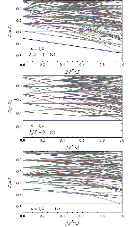
Figure 3: Exact spectrum (scaled energy per pair) of a spin $1/2$ cyclic chain with $XXZ$ first and second neighbor couplings in an alternating field (top panel in Fig. 2, Eqs. (80)–(81) and (G.1)), as a function of the relative strength $2J^{D}/J=\sin\xi$ (second to first neighbor $XX$ strength ratio in the linear chain), for $N=8$ spins and different values of $J_{z}$. In the vertical axis $n=N/2$ is the number of pairs and $E_{0}=JJ^{E}/2J^{D}=J/\sin\xi$, coinciding with the value of $J_{z}$ (Eq. (85)) in the bottom panel. The thick blue line depicts the energy of the dimerized GS in all panels.

In Fig. 3 we show illustrative results for the exact spectrum of an $N=8$ spin $1/2$ cyclic uniform chain (see Fig. 2 of main body) with $J^{E}=J$, $J^{E}_{z}=J_{z}$, for different values of $J_{z}$, as a function of the relative strength $2J^{D}/J=\sin\xi$. The energies are scaled to twice the pair energy at $J_{z}=0$, $E_{0}=JJ^{E}/2J^{D}=J/\sin\xi$, such that the ratio remains finite for $J^{D}\rightarrow 0$ (and constant for $J_{z}=0$), with $E_{0}$ coinciding with $J_{z}$ in the bottom panel (Eq. (86)).

It is first verified that in all cases the present dimerized state, which is a degenerate GS at zero field ($2J^{D}/J^{E}=1$), remains as a nondegenerate GS in the whole interval $0\leq 2J^{D}/J^{E}\leq 1$, well detached from the remaining spectrum, for both $J_{z}=J$ and $J_{z}=0$ (top and central panels). This holds also for the varying $J_{z}$ of Eq. (85) (bottom panel) necessary for $s_{p}\geq 1$. We notice that in the $2J^{D}/J^{E}\rightarrow 0$ limit just the field and $J_{z}$ terms remain in $H/E_{0}$, leading to a diagonal Hamiltonian in the standard basis.

The splitting of the degenerate dimerized GSs as $2J^{D}/J^{E}$ becomes lower than $1$ is seen to be initially linear in $2J^{D}/J^{E}$ in Fig. 1. This is due to the fact that according to Eq. (86), the scaled energy per pair of the dimerized state is $E/E_{0}=-\frac{1}{2}(1+J_{z}J^{D}/JJ^{E})$, constant for $J_{z}=0$ or $J_{z}$ given by Eq. (85), while for the orthogonal state at zero field, $\delta E\approx 0$ at first order in $1-2J^{D}/J^{E}$ and hence $E/E_{0}\approx-\frac{1}{2}(1+J_{z}/J)J^{D}/J^{E}$ per pair at this order, having then a larger slope.

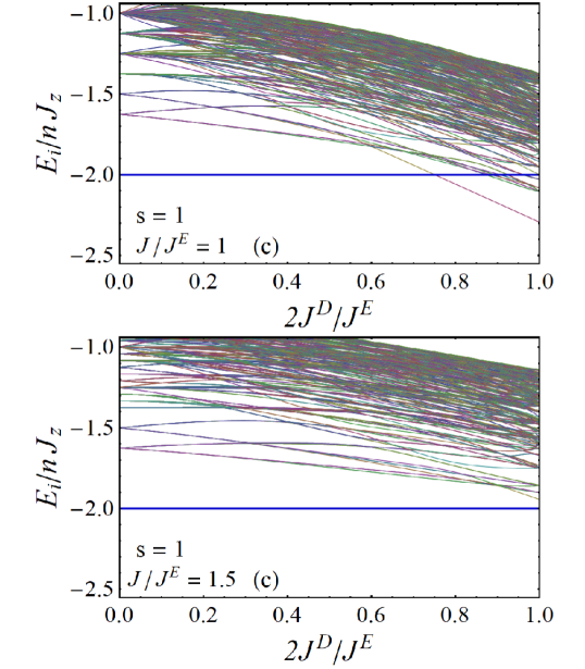
Figure 4: Exact energy spectrum of a cyclic $N=8$ spin $1$ chain with $XXZ$ couplings in an alternating magnetic field (Eq. (G.1)), for two different values of $J/J^{E}$ of the internal/interpair coupling ratio. The thick horizontal blue line corresponds to the energy (86) of the dimerized eigenstate, which becomes GS for sufficiently small $J^{D}/J$ even in the uniform case $J/J^{E}=1$ (top panel), where it is not GS at zero field ($2J^{D}/J^{E}=1$).

On the other hand, results for an $N=8$ spin $1$ chain ($s_{p}=1$) are shown for the cyclic (Fig. 4) and open (Fig. 5) cases. Here the internal $J_{z}$ should have the value (85) for dimerization. It is first seen that for $J^{E}_{\mu}=J_{\mu}$, the dimerized eigenstate (which is exactly the same in the cyclic and open cases for any spin), while not GS at $2J^{D}/J^{E}=1$ (zero field), does become GS for smaller $2J^{D}/J^{E}$, i.e.  sufficiently strong finite field. It is also confirmed in the lower panel that if the internal/interpair coupling ratio $J_{\mu}/J^{E}_{\mu}$ is increased the dimerized eigenstate becomes GS also at $2J^{D}/J^{E}=1$ (zero field ), with $J/J^{E}=1.5$ sufficient in the case considered. In the open case the threshold ratio for a dimerized GS at zero field decreases slightly for finite sizes, due to the smaller number of interpair connections.

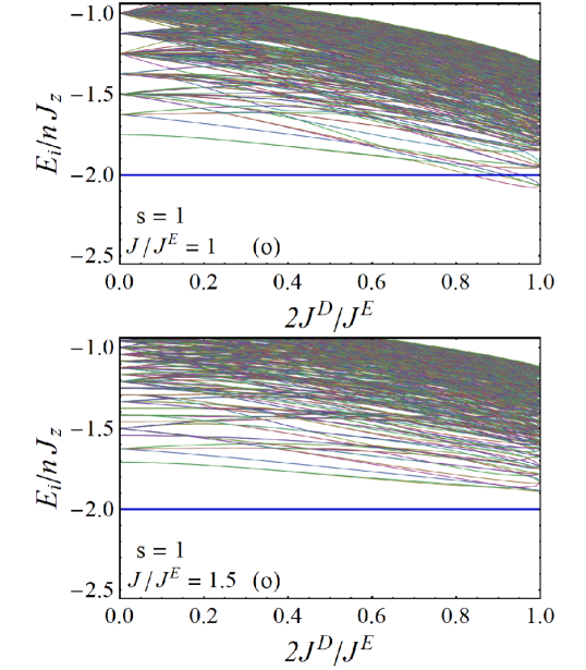
Figure 5: Exact spectrum of an open $N=8$ spin $1$ chain with $XXZ$ couplings. The details are similar to those of the previous figure.

G.2 Field induced dimerization in $XYZ$ systems

Starting from the generalized singlet $|\psi_{p}^{-}\rangle\equiv|\psi_{p}\rangle$ of Eq. (13), the factorizing equations for a product state $|\Psi^{+}\rangle=\otimes_{p}|\psi_{p}^{+}\rangle$, with $|\psi_{p}^{+}\rangle=e^{-i\pi S^{2_{p}}_{x}}|\psi_{p}^{-}\rangle$ can be obtained from those for $|\Psi^{-}\rangle$ (Eq. (9) for $\mu=\nu=z$ and (16) for $\mu,\nu=\pm$) replacing $J^{i_{p}j_{q}}_{y,z}\rightarrow(-1)^{i-j}J^{i_{p}j_{q}}_{y,z}$, and hence $J^{E^{\nu}_{pq}}_{\pm}\rightarrow J^{E^{\nu}_{pq}}_{\mp}$ for $\nu=\pm$, with $J^{D^{\nu}_{pq}}_{\pm}$ unchanged. Here

$$J^{E^{\nu}_{pq}}_{\pm}=\tfrac{J^{1_{p}2_{q}}_{\pm}+\nu J^{2_{p}1_{q}}_{\pm}}{2}\,,\;\;J^{D^{\nu}_{pq}}_{\pm}=\tfrac{J^{1_{p}1_{q}}_{\pm}+\nu J^{2_{p}2_{q}}_{\pm}}{2}$$ (88)

with $J^{i_{p}j_{q}}_{\pm}=J^{i_{p}j_{q}}_{x}\pm J^{i_{p}j_{q}}_{y}$. Then Eq. (4b) becomes, for $\xi_{p(q)}=\xi^{+}_{p(q)}$,

$$\!\!\!\!\!\!\!\!\!\!\!\!\!\!\!\!\!\!\!\sin\tfrac{\xi_{q}\pm\xi_{p}}{2}(J^{1_{p}1_{q}}_{+}\!\pm\!J^{2_{p}2_{q}}_{+})\! = \!\cos\tfrac{\xi_{q}\mp\xi_{p}}{2}(J^{1_{p}2_{q}}_{-}\!\pm\!J^{2_{p}1_{q}}_{-}),\;$$ (89a)

$$\!\!\!\!\!\!\!\!\!\!\!\!\!\!\!\!\!\!\!\cos\tfrac{\xi_{q}\mp\xi_{p}}{2}(J^{1_{p}1_{q}}_{-}\!\pm\!J^{2_{p}2_{q}}_{-})\! = \!\sin\tfrac{\xi_{q}\pm\xi_{p}}{2}(J^{1_{p}2_{q}}_{+}\!\pm\!J^{2_{p}1_{q}}_{+}),\;$$ (89b)

$$J^{1_{p}1_{q}}_{z}+J^{2_{p}2_{q}}_{z}=-(J^{1_{p}2_{q}}_{z}+J^{2_{p}1_{q}}_{z})\,,\;\,$$ (90)

with constraints (17) remaining unchanged. Notice that in both cases the constraints (17) in $XYZ$ systems can also be written as

$$(J^{D^{\pm}_{pq}}_{x})^{2}-(J^{D^{\pm}_{pq}}_{y})^{2}=(J^{E^{\pm}_{pq}}_{x})^{2}-(J^{E^{\pm}_{pq}}_{y})^{2}\,.$$ (91)

The corresponding Eqs.(89) for uniform or flipped alternating solutions become

$$\sin\xi = J^{E^{+}_{pq}}_{-}/J^{D^{+}_{pq}}_{+}\;\;(\xi_{p}=\xi_{q}=\xi)\,,$$ (92a)

$$\sin\xi = J^{D^{+}_{pq}}_{+}/J^{E^{+}_{pq}}_{-}\;\;(\xi_{p}=\pi-\xi_{q}=\xi)\,,$$ (92b)

for $J^{(D,E)^{-}_{pq}}_{-}=0$ in (92a), $J^{(D,E)^{-}_{pq}}_{+}=0$ in (92b).

Finally, for a mixed parity product $|\psi_{p}^{+}\rangle|\psi_{q}^{-}\rangle$, one should just replace $J^{2_{p}j_{q}}_{y,z}\rightarrow-J^{2_{p}j_{q}}_{y,z}$ $\forall\,j$ in the factorizing conditions (16)–(17) (and (9) for $\mu=\nu=x$), with all other couplings remaining unaltered. Then $J^{D^{\pm}_{pq}}_{y}\rightarrow J^{D^{\mp}_{pq}}_{y}$, $J^{E^{\pm}_{pq}}_{y}\rightarrow J^{E^{\mp}_{pq}}_{y}$ in (91), with (89)–(90) becoming

$$\!\!\!\!\!\!\!\!\!\!\!\!\!\!\!\!\sin\tfrac{\xi_{q}\pm\xi_{p}}{2}(J^{1_{p}1_{q}}_{+}\!\pm\!J^{2_{p}2_{q}}_{-})\! = \!\cos\tfrac{\xi_{q}\mp\xi_{p}}{2}(J^{1_{p}2_{q}}_{+}\!\pm\!J^{2_{p}1_{q}}_{-}),\;$$ (93a)

$$\!\!\!\!\!\!\!\!\!\!\!\!\!\!\!\!\cos\tfrac{\xi_{q}\mp\xi_{p}}{2}(J^{1_{p}1_{q}}_{-}\!\pm\!J^{2_{p}2_{q}}_{+})\! = \!\sin\tfrac{\xi_{q}\pm\xi_{p}}{2}(J^{1_{p}2_{q}}_{-}\!\pm\!J^{2_{p}1_{q}}_{+}),\;$$ (93b)

$$\!\!\!\!\!\!\,J^{1_{p}1_{q}}_{z}-J^{2_{p}2_{q}}_{z}=J^{1_{p}2_{q}}_{z}-J^{2_{p}1_{q}}_{z}\,.\;\;\;\;\;\;$$ (94)

In all cases these conditions ensure that the dimerized state $|\Psi\rangle=\otimes_{p}|\psi_{p}^{\sigma_{p}}\rangle$ will satisfy

$$V_{pq}|\Psi\rangle=0\,.$$ (95)

If valid $\forall\,p\neq q$, $|\Psi\rangle$ will then be eigenstate of $H$ iff $\forall\ p$,

$$H_{p}|\psi_{p}^{\sigma_{p}}\rangle=E_{p}^{\sigma_{p}}|\psi_{p}^{\sigma_{p}}\rangle\,.$$ (96)

For $s_{p}=1/2$, this just requires adjusting the fields through the expression given in the main-body, leaving $b^{1_{p}}-\sigma_{p}b^{2_{p}}$ free. For $s_{p}\geq 1$ we should have in addition

$$J^{p}_{x}=-\sigma_{p}J^{p}_{y}=\sigma_{p}J^{p}_{z}\sin\xi_{p}$$ (97)

in the internal hamiltonian, with $b^{1_{p}}=-\sigma_{p}b^{2_{p}}$.

The total energy of the dimerized state is therefore $E=\sum_{p}E_{p}^{\sigma_{p}}$, with the pair energy $E_{p}^{\pm}$ given by

$$E_{p}^{\pm}=\left\{\begin{array}[]{rcl}\tfrac{1}{4}\left(-\frac{J^{p}_{x}\mp J^{p}_{y}}{\sin\xi^{\pm}_{p}}\pm J^{p}_{z}\right)&,&s_{p}=1/2\\ \pm s_{p}(s_{p}+1)J_{z}&,&s_{p}\geq 1\end{array}\right.\,.$$ (98)

For uniform dimerization, we consider uniform internal anisotropic couplings $J^{p}_{\mu}=J_{\mu}$ and fields $b^{i_{p}}=B_{i}$ $\forall\,p$, with interpair couplings

$$J^{i_{p}j_{q}}=r_{pq}[\delta_{ij}J^{D}_{\mu}+(1-\delta_{ij})J^{E}_{\mu}]\,,$$ (99)

for $i,j=1,2$ (top panel in Fig. 2 of main-body), where $r_{pq}\geq 0$ determines its range. We will set $J_{x}\geq|J_{y}|$ and $J^{D}_{x}\geq J^{E}_{x}\geq|J^{E}_{y}|$ with $J^{D}_{y}\geq 0$, such that the constraint (91) implies $J^{D}_{x}\geq J^{D}_{y}\geq|J^{E}_{y}|$. We also set $J^{D}_{z}=J^{E}_{z}=0$, such that constraints (9) for $\mu=\nu=z$ are trivially satisfied for both parities and

$$H = \sum_{p}\;B_{1}S_{1_{p}}^{z}+B_{2}S_{2_{p}}^{z}+\sum_{\mu=x,y,z}J_{\mu}S_{1_{p}}^{\mu}S_{2_{p}}^{\mu}$$

$$+\sum_{p<q}r_{pq}\!\sum_{\mu=x,y}\left(J^{E}_{\mu}(S_{1_{p}}^{\mu}S_{2_{q}}^{\mu}+S_{2_{p}}^{\mu}S^{\mu}_{1_{q}})\right.$$

$$\left.\hskip 62.59596pt+J^{D}_{\mu}(S_{1_{p}}^{\mu}S^{\mu}_{1_{q}}+S^{\mu}_{2_{p}}S^{\mu}_{2_{q}})\right).$$

Hence, for $s_{p}=1/2$, coexisting uniform opposite parity “vertical” dimerized eigenstates

$$|\Psi^{\pm}\rangle=\otimes_{p}|\psi^{\pm}_{p}(\xi^{\pm})\rangle\,,$$ (101)

with $|\psi_{p}^{\pm}(\xi)\rangle$ of the form (18), become feasible for angles $\xi_{p}^{\pm}=\xi^{\pm}$ determined by the interpair couplings through Eqs. (92a)-(16a):

$$\sin\xi^{\pm}=\frac{J^{E}_{\mp}}{J^{D}_{+}}=\frac{J^{E}_{x}\mp J^{E}_{y}}{J^{D}_{x}+J^{D}_{y}}\,.$$ (102)

Previous settings ensure $0\leq J^{E}_{\mp}/J^{D}_{+}\leq 1$. The upper and lower uniform dimerizing fields $B_{i}=b_{i}^{p}$ are then determined from $b^{2_{p}}\pm b^{1_{p}}=\tfrac{1}{2}(J^{p}_{y}\mp J^{p}_{x})\cot\xi_{p}^{\pm}$, i.e.  $B_{{}^{1}_{2}}=\tfrac{B_{+}\pm B_{-}}{2}$, with

$$B_{\pm}=-\tfrac{1}{2}(J_{x}\mp J_{y})\cot\xi^{\pm}\,,$$ (103)

such that $|\psi_{p}^{\pm}(\xi^{\pm})\rangle$ are also simultaneous eigenstates of the internal Hamiltonian $H_{p}$ with pair energies (98).

Since the present settings imply $E_{p}^{\pm}<0$ for $J_{z}=0$, $|\psi_{p}^{+}\rangle$ ($|\psi_{p}^{-}\rangle$) will be the GS of $H_{p}$ for $J_{z}<0$ ($J_{z}>0$). The energies of these uniform vertical dimerized states are then $E^{\pm}=nE_{p}^{\pm}$, with $n=2N$ the number of pairs. Therefore, $|\Psi^{+}\rangle$ ($|\Psi^{-}\rangle$) will always be the GS of the full $H$ for sufficiently large $J_{z}>0$ ($J_{z}<0$), their threshold values depending on the strength and range (so far arbitrary) of the interpair couplings, determined by $r_{pq}$.

As a specific example, let us consider the case of a tetramer ($n=2$, $p=1$, $q=2$), with $J^{E}_{\mu}=J_{\mu}$ for $\mu=x,y$. Then, using (102), the pair energies (98) and fields (103) become

$$E_{p}^{\pm} = -\tfrac{1}{4}[J^{D}_{x}+J^{D}_{y}\mp J_{z}]\,,$$ (104)

$$B_{\pm} = -\tfrac{1}{2}(J_{x}^{D}+J_{y}^{D})\cos\xi^{\pm}\,,$$ (105)

with $E_{p}^{\pm}$ independent of $J_{x,y}$.

Remarkably, in this case an “horizontal” mixed parity dimerized exact eigenstate $|\Psi^{+-}\rangle=|\psi^{\prime+}_{1_{p}1_{q}}\rangle|\psi^{\prime-}_{2_{p}2_{q}}\rangle$ becomes also feasible for the same previous couplings and fields, according to the corresponding version of Eqs. (93)–(94) and (91) (internal couplings $J^{1_{p}2_{p}}_{\mu}\rightarrow J^{D}_{\mu}$, interpair couplings $J^{i_{p}i_{q}}_{\mu}\rightarrow J_{\mu}$, $J^{i_{p}j_{q}}\rightarrow J^{E}_{\mu}=J_{\mu}$). The states $|\psi^{\prime\pm}_{i_{p}i_{q}}\rangle$ have again the form (18) with angles $\xi^{\prime\pm}$ determined from the corresponding Eq. (103), $\tan\xi^{\prime\pm}=-\frac{1}{2}J^{D}_{\mp}/B^{\prime}_{\pm}$, implying $\xi^{\prime-}=\frac{\pi}{2}$ and

$$\tan\xi^{\prime+}=-\tfrac{1}{4}\tfrac{J^{D}_{x}-J^{D}_{y}}{B_{1}}\,.$$ (106)

For these angles the corresponding dimerizing Eqs. (93)-(94) are directly satisfied.

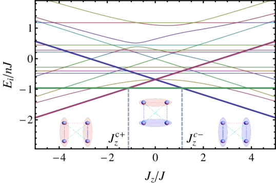
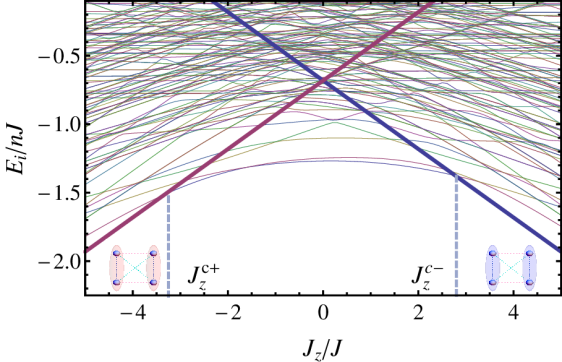
Figure 6: Top: Exact spectrum (energy per pair in units of the strength $J=J_{x}$) and GS phase diagram of an $N=4$ spin $1/2$ system with $XYZ$ couplings in a nonuniform field (example 2 of main body), as a function of $J_{z}/J$ for $J_{y}=J_{x}/2$. The vertical dashed lines delimit the sectors $J_{z}<J_{z}^{c+}$, $J_{z}^{c+}<J_{z}<J_{z}^{c-}$ and $J_{z}>J_{z}^{c-}$, for which three distinct dimerized exact GSs arise: “vertical” and uniform in the outer sectors, with states $|\psi_{p}^{+}\rangle$ for $J_{z}<J_{z}^{c+}$ (pink dimers, thick red line), and states $|\psi_{p}^{-}\rangle$ for $J_{z}>J_{z}^{c-}$ (blue dimers, thick blue line), while “horizontal” with different upper and lower states $|{\psi_{p}^{\prime}}^{+}\rangle$, $|{\psi_{p}^{\prime}}^{-}\rangle$) in the central sector (pink and blue dimers, thick green line). These dimerized states of the tetramer are exact eigenstates of the Hamiltonian $\forall\,J_{z}$. The critical values $J_{z}^{c\pm}=\mp J_{z}^{c}$ are determined by Eq. (108). Bottom: The spectrum of an $N=8$ spin $1/2$ system for the same couplings (same scaling). The GS in the outer sectors $J_{z}<J_{z}^{c+}$ and $J_{z}>J_{z}^{c-}$ is again exactly dimerized with states $|\psi_{p}^{+}\rangle$ (left, pink dimers, thick red line) and $|\psi_{p}^{-}\rangle$ (right, blue dimers, thick blue line). The pair states involved are the same as those in the top panel.

Using (91), (98) and (105)–(106), the total energy of this “horizontal” dimerized state can be written as

$$E^{\prime+-} = -\tfrac{1}{4}\left(\tfrac{J^{D}_{x}-J^{D}_{y}}{\sin\xi^{\prime+}}+J^{D}_{x}+J^{D}_{y}\right)$$ (107)

$$= -\tfrac{1}{4}(J^{D}_{x}+J^{D}_{y})(\cos\xi^{+}\cos\xi^{-}+2)$$

$$= -\tfrac{1}{2}(\sqrt{{J_{x}^{D}}^{\,2}-J_{x}^{2}}+J^{D}_{x}+J^{D}_{y})\,,$$

being then independent of $J_{y}$ and $J_{z}$, and lower than $2E_{p}^{\pm}$ at $J_{z}=0$. Therefore, $|\Psi^{\prime+-}\rangle$ will be the GS in an interval $J_{z}^{c+}<J_{z}<J_{z}^{c-}$, with $J_{z}^{c\pm}=\mp J_{z}^{c}$ and

$$J_{z}^{c}=\sqrt{{J_{x}^{D}}^{\,2}-J_{x}^{2}}\,,$$ (108)

whereas the “vertical” dimerized states $|\Psi^{\pm}\rangle$ will be GS for $J_{z}<-J_{z}^{c}$ ($|\Psi^{+}\rangle$) and $J_{z}>J_{z}^{c}$ ($|\Psi^{-}\rangle$). For the present settings ($\xi^{\pm}\in[0,\pi/2]$) the upper field $B_{1}$ is stronger than the lower field ($|B_{1}|>|B_{2}|$) and hence it is the upper pair which is in the state $|{\Psi^{\prime}}^{+}\rangle$ in the intermediate horizontal dimerized state. A similar flipped eigenstate $|\Psi^{\prime-+}\rangle$ obviously arises for flipped fields and angles.

The top panel in Fig. 6 shows the tetramer spectrum as a function of $J_{z}$ in the case $J_{y}=\frac{1}{2}J_{x}$ and $J^{D}_{x}=\frac{3}{2}J_{x}$, with $J_{x}=J$ and $r_{12}=1$. The three distinct dimerized GS phases are easily identified as the three lowest straight lines that intersect at the critical $J_{z}$ values $\pm J_{z}^{c}=\pm 1.118J$ (Eq. (108)) and delimit these phases. Notice, however, that for other levels, the spectrum is not necessarily symmetric as a function of $J_{z}$.

The lower panel in Fig. 6 depicts the spectrum of an $N=8$ spin $1/2$ array ($n=4$ pairs) as a function of $J_{z}$, for the same coupling strengths and first neighbor interpair couplings ($r_{pq}=\delta_{q,p+1}$) with cyclic conditions ($n+1\equiv 1$). As predicted, the outer vertical dimerized GS phases, whose energies are again characterized by straight lines, arise for sufficiently large $|J_{z}|$ (here $J_{z}^{c-}\approx 2.8J$, $J_{z}^{c+}\approx-3.25J$). The central sector, however, corresponds now to an entangled non-dimerized phase. Similar results are obtained in an open system (with slightly lower values of $|J_{z}^{c\pm}|$) or with longer range interpair couplings (larger $|J_{z}^{c}|$).

Analogous “vertical” dimerized GSs also arise $\forall$ spin $s_{p}$ with the generalized singlet states $|\psi_{p}^{-}\rangle$ of Eq. (13) for $J_{z}>J_{z}^{c-}$ and its partner state $|\psi_{p}^{+}\rangle=e^{-i\pi S^{x}_{2_{p}}}|\psi_{p}^{-}\rangle$ for $J_{z}<J_{z}^{c+}$, for sufficiently large internal couplings satisfying Eq.  (97). This implies now a fixed $J_{z}/J_{x}$ ratio depending on $\xi^{\pm}$ and $J_{y}=\mp J_{x}$ for the internal couplings. Hence $|\psi^{\pm}\rangle$ are no longer coexisting eigenstates. These conditions can be relaxed for a more general internal $H_{p}$.