akshay.koottandavida@yale.edu
ioannis.tsioutsios@yale.edu††thanks: These authors contributed equally to this work.
akshay.koottandavida@yale.edu
ioannis.tsioutsios@yale.edu††thanks: michel.devoret@yale.edu
Supplementary Information
“Erasure detection of a dual-rail qubit encoded in a double-post superconducting cavity”
††preprint: APS/123-QED
I Experimental setup and sample parameters
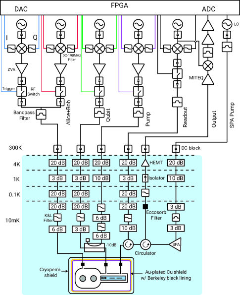
Our experimental system consists of a coaxial stub cavity [1] with two posts, made of 5N Aluminium treated with a chemical etch to improve surface quality. The two harmonic oscillators are the two lowest frequency normal modes of the system obtained by the hybridisation of the modes of the individual stubs. The auxiliary transmon [2] made of Aluminium is fabricated on a sapphire chip along with a readout resonator and a Purcell filter [3]. The chip is inserted into a tunnel waveguide that connects to the storage cavity modes and is held in place on one side using copper clamps. The entire package is rigidly attached to a gold-plated copper bracket that is mounted on to the base plate of a dilution refrigerator. The bracket is surrounded by a gold-plated copper can, coated with a thin layer of Berkeley black on the inside to absorb high frequency photons. The outer Cryoperm shield attenuates stray magnetic fields. The top of this can is sealed with a lid with SMA feedthroughs and each seam is sealed with Indium wires.
Control pulses for the relevant modes are synthesized via Digital-Analog Converters (DACs) from a Field Programmable Gate Array (FPGA) with a baseband of DC-250MHz [4]. These signals are up-converted to the required frequencies using IQ mixers and local oscillators (LO) which are then amplified and filtered accordingly. Fast RF switches are used to gate the signals in each line. These are then sent into different microwave lines in the dilution refrigerator each with different attenuation and filtering such that the noise temperature at relevant frequencies are around base plate temperature (20mK). Readout signals are amplified via a quantum-limited SNAIL(Superconducting Nonlinear Asymmetric Inductive eLement) parametric amplifier(SPA) [5, 6], with a pump-port filter designed for efficient pump delivery. This amplified signal is further amplified by HEMT (High Electron Mobility Transistor) amplifier at the 4K stage and further by room temperature amplifier. This signal is then down-converted to a 50MHz signal using an IR mixer and the same LO used to up-convert the input readout pulse. After appropriate filtering and amplification, the Analog-Digital Converter(ADC) of the FPGA digitises, demodulates and integrates to obtain a readout value.
| Alice | Frequency | |
| Cross-Kerr shift | ||
| Relaxation | ||
| Dephasing | ||
| Thermal population | ||
| Bob | Frequency | |
| Cross-Kerr shift | ||
| Relaxation | ||
| Dephasing | ||
| Thermal population | ||
| Transmon | Frequency | |
| Anharmonicity | ||
| Relaxation | ||
| Dephasing (Ramsey) | ||
| Dephasing (Echo) | ||
| Thermal population | ||
| Readout | Frequency | |
| Cross-Kerr shift | ||
| Coupling strength | ||
| Internal loss |
II Cross-Kerr tuning
II.1 Deriving the effective Hamiltonian
We begin by writing the Hamiltonian of the Alice-Bob-Transmon system with a linear drive on the transmon delivered via a capacitively coupled port. Up to the leading order in the cosine potential of the Josephson junction, the Hamiltonian is
| (1) |
where is the frequency of the mode representing Alice, Bob, transmon and the drive, respectively, and is the coefficient of the th order term representing the Josephson energy. First we perform a displaced frame transformation on the qubit to absorb the drive into the 4th order term. The Hamiltonion becomes
| (2) |
where and . Choosing the displacement such that , ignoring terms oscillating at , we can write the Hamiltonian in the displaced frame, up to constant terms, as
| (3) |
Next we move into a frame where the modes are rotating at their bare frequencies. We add a slight detuning to Bob from its bare detuning (adding this detuning on the transmon has equivalent resolt). The unitary for this transformation is then, and we get the interaction Hamiltonian
| (4) |
where represents the hermitian conjugate of all the terms in the rounded brackets preceding it. For the cross-Kerr tuning process we drive a 2-photon transition at the frequency . Substituting this in to the above Hamiltonian and collecting all the static terms from the expansion of the th order term, with the rotating wave approximation(RWA) applied, we get
| (5) |
where, is the Stark-shift and is the self-Kerr of the -th mode and is the cross-Kerr between modes and . In the first line in the above equation, is the interaction rate of the cross-Kerr tuning process, detuned by . Going into the interaction frame with respect to the transmon self-Kerr , we get
| (6) |
By choosing and moving into the appropriate rotating frame, we can selectively pick out the transition to address and ignore the other pumped terms under the RWA(). Hence, we get,
| (7) |
where we’ve redefined the drive amplitude to and dropped the negligible terms like the self-Kerr rates of the cavities and the cross-Kerr between them. Note that the pump frequency is . By diagonalizing the above pumped Hamiltonian, we obtain the behavior of the combined Fock states, as seen from the fits in Fig1.(c) of the main text.
To get an intuition of how the above Hamiltonian modifies the cross-Kerr, let us consider the transmon coupled to just Bob, expand in the Fock basis and select only the term that couples . Here we write a simplified form of the above Hamiltonian for this term,
| (8) |
This describes two levels coupled to each other and we can diagonalize easily to find the eigenvalues and eigenstate. The eigenvalues are . For the limit of , the lowest eigenvalue can be approximated to the lowest order as and the corresponding eigenstate is . For large detunings, the hybridisation is weak and if the level of the transmon is never occupied, then we can approximately rewrite the Hamiltonian as
| (9) |
This corresponds to modified bare energy of the state. If we now perform the same for higher Fock states it will result in modified cross-Kerr due to the drive.
II.2 Characterizing the cross-Kerr tuning process
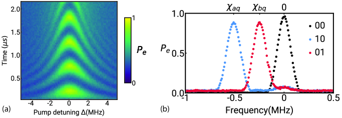
To characterize the cross-Kerr tuning, we prepare either of the cavities in the state and the transmon in . By applying the cross-Kerr pump with varying frequency and time, we measure the probability of the transmon to be in . This reveals the chevron between the levels and with a Rabi rate . We use this method to calibrate the strength and the stark-shifted centre frequency of the process, for either cavity modes using Eq. 6. Fig.S 2a shows the chevron pattern of such an oscillation perform on the Bob cavity.
II.3 Gaussian pulse for erasure detection
Fig.S 2b shows transmon spectroscopy results obtained after preparing the cavities in and states. The spectroscopy is performed using a Gaussian pulse with , with a total duration of . This is the same pulse used in the erasure detection circuit.
III Dual-rail qubit
III.1 Encoding and error-channels
We define the dual-rail qubit in the joint-Hilbert space of Alice and Bob. The logical codewords are and . Here the first mode in the ket is Alice and the second is Bob. The full error set for the code due to error channels of the cavities is . These represent the identity, cavity photon loss, cavity photon gain, cavity dephasing and the no-jump error channels respectively. The -th error channel will act on an arbitrary state in the logical codespace, , and take the system into the error space as follows,
| (10) |
where is the -th error channel in the set . From this, it becomes apparent that the error state for the photon loss channel, in either Alice or Bob, is the ground state of the system : . For the photon gain channels, we have
| (11) |
| (12) |
Note that for both the photon gain channels the total excitation in the cavities is 2. Dephasing error channel of the individual cavities will lead to dephasing within the dualrail codespace. Finally, there will be a backaction on the codespace due to the no-jump evolution of the states which will look like
| (13) |
where is the difference in loss rates between the two modes. This no-jump evolution causes the state to be polarised to the longer lived mode, distorting the encoded information.
III.2 Erasure detection and trajectories
III.3 Hidden Markov decoding
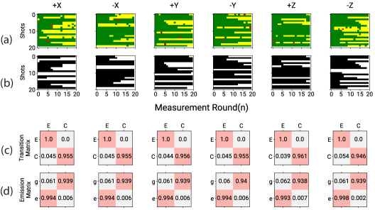
To predict cavity photon loss and the most likely state of the system, we train a Categorical Hidden Markov Model (HMM) with the experimentally obtained trajectories. The HMM assumes 2 hidden states, Codespace and Errorspace and 2 measurement outcomes and . The transition matrix element determines the probability of the system to make a transition from state in the current time step. Similarly, the emission matrix element is the probability of observing the measurement outcome given that the system is in state at the current time step. In our experiment, we measure trajectories for each of the 6 cardinal states in the dual-rail Bloch sphere and train an HMM for each state to learn the probabilities. Each trajectory is 167 measurement rounds long. Fig.S 3a shows a sample of these trajectories for the 6 cardinal states while Fig.S 3b shows the decoded trajectories as predicted by the HMM. Fig.S 3c and Fig.S 3d depicts the transition and emission matrices obtained after the training on the raw trajectories. Since each erasure detection round is long, we can convert these probabilities in to rates.
| State | Erasure prob. | Erasure rate |
|---|---|---|
| per gate | ||
| per gate | ||
| Equator states | per gate | |
We expect the erasure rates to be and for the states and for the states on the equator. The HMM predicted values matches well with the rates extracted independently(from Table 1). The HMM also allows us to extract false positive and false negative probabilities.
| (14) |
The above values are averaged over all 6 cardinal states.
IV Joint-Wigner tomography
IV.1 Logical Pauli measurements
To extract the expectation values of the logical Pauli operators of the dual-rail subspace, we sample specific points in the joint-Wigner space of the cavities [7, 8]. To see this, we first define describe how to measure the expectation values of the logical Pauli operators for the Fock qubit using single-mode Wigner. We will then extend this method to measure the logical Pauli operators of the dual-rail qubit using Joint-Wigner.
IV.1.1 Fock qubit
The single mode Wigner for a bosonic mode is defined as
| (15) |
where is the displaced parity operator with being the parity operator for the mode. The logical codewords for the Fock qubit are and . We then proceed to project the displaced parity onto the fock qubit subspace using the identity projector . We get
| (16) |
Using Laguerre polynomials and the identity , we simplify the above equation to
| (17) |
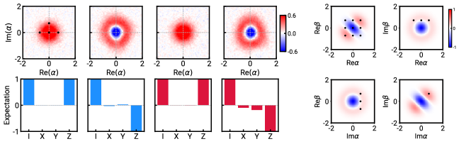
here we used and . We then equate the above equation to the 4 Pauli operators and solving for , we get . This tells us that if we restrict ourselves to the Fock qubit subspace then we only need to measure these four points in phase space to reconstruct the full density matrix. Fig.S 4a, shows the pictorially the four points in phase space and also provides intuition to why we expect it. Now, using these displacements, we can invert the above equation to get the Pauli operators as
| (18) |
IV.1.2 Dual-rail qubit
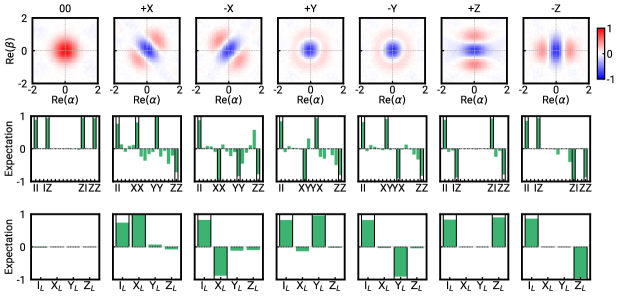
We can easily extend this technique for our dual-rail qubit. Crucially, we will have to measure the joint-Wigner, defined as,
| (19) |
where we define the displaced joint parity operator as . We first note that we cannot directly project on to the dual-rail subspace since, due to erasure errors, the system leaks out of this subspace. In order to incorporate the error state , we instead choose to restrict ourselves on to the two qubit subspace spanned by Fock qubit in both Alice and Bob : . The dual-rail subspace, including the error space, lives within this larger space, even though we have some states we are not concerned with. Now, projecting the displaced joint parity onto this subspace, we get,
| (20) |
which we then equate to the 16 two-qubit Paulis . Its easy to see that this will yield 16 points, which are just combinations of the 4 points from single-mode displacements that we derived above. We write this set of 16 displacements explicitly below,
| (21) |
We will denote as the -th element in the above set, with . From these displacements, we can construct the 16 two-qubit Pauli matrices as follows,
| (22) |
For our purposes, we only care about the Pauli operators for the dual-rail, which can be obtained by linear combinations of the above matrices, since we work in the basis. Therefore, the logical Pauli operators for the dual-rail qubit are
| (23) |
IV.2 Dual-rail Pauli transfer matrix with erasure detection
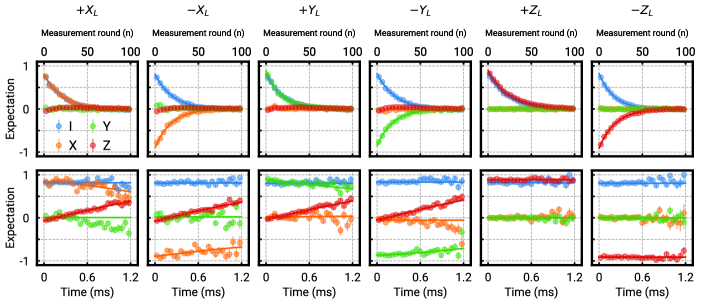
We measure the expectation values of the Pauli operators after preparing the 6 cardinal states as a function of number of erasure detection rounds. Top panel in Fig.S 6 shows the measured values with exponential fits. The decay of the identity operator clearly shows leakage outside of the codespace. The bottom panel shows postselected data. The postselected looks constant and we can only obtain an upper bound on residual leakage rate by fitting to an exponential decay . We then fit the postselected and to extract dephasing rates within the dualrail subspace. Taking into account the no-jump evolution, the analytical formula for the evolution of these operators will look like [9]
| (24) |
| (25) |
| (26) |
for an arbitrary state . On top of this, we add an exponentially decaying term to calculate residual dephasing and bit-flip rate within the codespace. We observe that the fits agree well with the measured data. We note that the increase in for the equator states shows the polarisation of the Bloch vector towards the longer lived cavity (Bob) due to the no-jump backaction.
References
- Reagor et al. [2013] M. Reagor, H. Paik, G. Catelani, L. Sun, C. Axline, E. Holland, I. M. Pop, N. A. Masluk, T. Brecht, L. Frunzio, M. H. Devoret, L. Glazman, and R. J. Schoelkopf, Reaching 10 ms single photon lifetimes for superconducting aluminum cavities, Applied Physics Letters 102, 192604 (2013).
- Koch et al. [2007] J. Koch, T. M. Yu, J. Gambetta, A. A. Houck, D. I. Schuster, J. Majer, A. Blais, M. H. Devoret, S. M. Girvin, and R. J. Schoelkopf, Charge-insensitive qubit design derived from the Cooper pair box, Physical Review A 76, 042319 (2007).
- Purcell et al. [1946] E. M. Purcell, H. C. Torrey, and R. V. Pound, Resonance Absorption by Nuclear Magnetic Moments in a Solid, Physical Review 69, 37 (1946).
- Reinhold [2019] P. Reinhold, , Ph.D. thesis (2019).
- Frattini et al. [2017] N. E. Frattini, U. Vool, S. Shankar, A. Narla, K. M. Sliwa, and M. H. Devoret, 3-wave mixing Josephson dipole element, Applied Physics Letters 110, 222603 (2017).
- Sivak et al. [2019] V. Sivak, N. Frattini, V. Joshi, A. Lingenfelter, S. Shankar, and M. Devoret, Kerr-Free Three-Wave Mixing in Superconducting Quantum Circuits, Physical Review Applied 11, 054060 (2019).
- Wang et al. [2016] C. Wang, Y. Y. Gao, P. Reinhold, R. W. Heeres, N. Ofek, K. Chou, C. Axline, M. Reagor, J. Blumoff, K. M. Sliwa, L. Frunzio, S. M. Girvin, L. Jiang, M. Mirrahimi, M. H. Devoret, and R. J. Schoelkopf, A Schrödinger cat living in two boxes, Science 352, 1087 (2016).
- Chapman et al. [2023] B. J. Chapman, S. J. de Graaf, S. H. Xue, Y. Zhang, J. Teoh, J. C. Curtis, T. Tsunoda, A. Eickbusch, A. P. Read, A. Koottandavida, S. O. Mundhada, L. Frunzio, M. Devoret, S. Girvin, and R. Schoelkopf, High-On-Off-Ratio Beam-Splitter Interaction for Gates on Bosonically Encoded Qubits, PRX Quantum 4, 020355 (2023).
- Teoh et al. [2023] J. D. Teoh, P. Winkel, H. K. Babla, B. J. Chapman, J. Claes, S. J. de Graaf, J. W. O. Garmon, W. D. Kalfus, Y. Lu, A. Maiti, K. Sahay, N. Thakur, T. Tsunoda, S. H. Xue, L. Frunzio, S. M. Girvin, S. Puri, and R. J. Schoelkopf, Dual-rail encoding with superconducting cavities, Proceedings of the National Academy of Sciences 120, e2221736120 (2023).