AI-accelerated Discovery of Altermagnetic Materials

Abstract

Altermagnetism, a new magnetic phase, has been theoretically proposed and experimentally verified to be distinct from ferromagnetism and antiferromagnetism. Although altermagnets have been found to possess many exotic physical properties, the very limited availability of known altermagnetic materials (e.g., 14 confirmed materials) hinders the study of such properties. Hence, discovering more types of altermagnetic materials is crucial for a comprehensive understanding of altermagnetism and thus facilitating new applications in the next generation information technologies, e.g., storage devices and high-sensitivity sensors. Here, we report 25 new altermagnetic materials that cover metals, semiconductors, and insulators, discovered by an AI search engine unifying symmetry analysis, graph neural network pre-training, optimal transport theory, and first-principles electronic structure calculation. The wide range of electronic structural characteristics reveals that various novel physical properties manifest in these newly discovered altermagnetic materials, e.g., anomalous Hall effect, anomalous Kerr effect, and topological property. Noteworthy, we discovered 8 $i$-wave altermagnetic materials for the first time. Overall, the AI search engine performs much better than human experts and suggests a set of new altermagnetic materials with unique properties, outlining its potential for accelerated discovery of the materials with targeting properties.

Keywords: altermagnetism, pre-trained model, symmetry analysis, material discovery

Introduction

Magnetic materials form a cornerstone of our modern information society. Generally, magnetism is categorized into ferromagnetism and antiferromagnetism. Recently, based on the spin group formalism, a new magnetic phase called altermagnetism has been theoretically proposed [1, 2], which exhibits numerous novel physical properties [1, 2, 3, 4, 5, 6, 7, 8, 9, 10, 11, 12], paving the path way of new avenues in the next generation of information technology. Both altermagnets and conventional antiferromagnets have compensated antiparallel spin sublattices resulting in vanishing net magnetic momentum. The compensated antiparallel spin sublattices are connected by the spin symmetry $\{T||IT\}$ or $\{C_{2}^{\perp}||\tau\}$ transformation for conventional antiferromagnets, but by the spin symmetry $\{C_{2}^{\perp}||R_{i}\}$ transformation for altermagnets [1]. Here, the symmetry operations at the left and right of the double vertical bar act only on the spin space and lattice space, respectively; the notation $C_{2}^{\perp}$ represents the $180^{\circ}$ rotation perpendicular to the spin direction; the notations $I,T,R_{i}$, and $\tau$ denote space inversion, time reversal, rotation/mirror, and fractional translation operations, respectively. Due to the absence of spin symmetry $\{T||IT\}$ or $\{C_{2}^{\perp}||\tau\}$, altermagnets have spin splitting in electronic bands. Unlike isotropic k-independent $s$-wave spin splitting in ferromagnets, altermagnets can form anisotropic k-dependent $d$-wave, $g$-wave, and $i$-wave spin splitting according to different spin group symmetry [1]. Moreover, altermagnets have not only spin-splitting bands deriving from the magnetic exchange interaction which is the same as ferromagnets but also unique extraordinary spin-splitting bands deriving from anisotropic electric crystal potential [1]. In some altermagnets, the spin splitting can even have magnitudes of $eV$ in parts of the Brillouin zone (BZ) [1, 2, 3]. The anisotropic k-dependent spin splitting can result in a unique spin current by electrical means in $d$-wave altermagnets [4]. Based on the unique spin current, the spin-splitter torque in $d$-wave altermagnets was proposed in theory [4] and confirmed by experiments [5, 6], which may circumvent limitations of spin-transfer torque (ferromagnets) and spin-orbit torque (conventional antiferromagnets or nonmagnetic materials with strong spin-orbit coupling) in magnetic memory devices [4]. Meanwhile, the giant and tunneling magnetoresistance can also be proposed in altermagnets based on the anisotropic k-dependent spin splitting [3]. In the relativistic case, the time-reversal symmetry-breaking macroscopic phenomena, including quantum anomalous Hall [7], anomalous Hall [8, 9], and anomalous Kerr effects [10], have been predicted by theories in altermagnets, moreover, the anomalous Hall effect has been supported by experiments [11, 12].

On the other hand, magnetic topological phases and their exotic physical properties have recently attracted intensive experimental and theoretical attention. Very recently, some topological semimetal and insulator phases protected by spin group symmetry have been proposed in theory [13, 14, 15]. Considering that the altermagnets are described by spin group symmetry and the symmetry landscape of spin space groups is more plentiful than that of the conventional magnetic space groups, more new magnetic topological phases and their exotic physical properties may be thus proposed theoretically in altermagnets. Nevertheless, altermagnets are hitherto in the early stage of research. Since there are many exotic physical properties that have been discovered and new physical phenomena to be discovered, altermagnets are bound to attract intensive theoretical and experimental attention in the near future. However, altermagnetic materials are known very limited so far (e.g., 14 confirmed materials [2] plus 4 supercell materials [16]). Hence, there is an urgent need to discover more altermagnetic materials for a comprehensive understanding of altermagnetism, thus facilitating new applications in the next generation of information technologies.

Conventional discovery methods primarily rely on screening in a large search space by human experts resorting to physics-based experience, which, as a result, is subjected to low efficiency and unsatisfactory accuracy. Meanwhile, artificial intelligence (AI) technology has found many key applications in the discovery of materials [17]. For instance, AI was used for predicting organic compound synthesis in organic chemistry [18], planning chemical synthesis pathways [19], iterative synthesis of small molecules [20], and accelerating the discovery of self-assembling peptides [21]. Recently, deep learning methods have been applied to the prediction of crystal materials with targeted properties [22, 23]. These methods generally utilize a large amount of crystal structure data to train graph neural network (GNN) models in an end-to-end manner, without explicit reference to the physical laws underlying these material properties. The trained model could predict key physical properties of crystal materials, such as formation energy and band gap, based on a rich training dataset containing over $10^{4}$ labeled samples [22]. However, such methods are no longer suitable for discovering altermagnetic materials, because of the fact that the known positive samples are extremely limited (e.g., 14 confirmed materials).

In this article, we introduce an AI search engine, as shown in Fig. 1, that combines advances in pre-trained model (GNN pre-training [24] and optimal transport theory [25]) and physics-based approaches (symmetry analysis and first-principles electronic structure calculation) to discover new altermagnetic materials under the condition of very limited labeled samples. First, based on symmetry analysis, we constructed the pre-training dataset (containing 68,116 materials), fine-tuning dataset (containing 25,605 materials, namely, 25,591 negative samples plus 14 positive samples), and candidate dataset (containing 42,525 materials) from the Material Project [26]. Next, we pre-trained a GNN model (composed of an encoder and a decoder) for crystal materials, based on optimal transport theory. Once the pre-training was done, we fine-tuned the encoder on the fine-tuning dataset to obtain a classifier model. Then, the structured material information from the candidate dataset was input into the classifier model to quantify the probability as an indicator of whether each material is an altermagnetic material. We filtered out the materials with probabilities greater than 0.9 as the candidate altermagnetic materials. Finally, we employed the first-principles electronic structure calculations to obtain a set of key properties of the candidate material to verify and confirm its altermagnetism. Furthermore, the confirmed altermagnetic materials were added to the fine-tuning dataset for an iterative process of fine-tuning and classifier prediction, reinforcing the predictability of the model. The efficacy of this AI search engine has been well demonstrated.

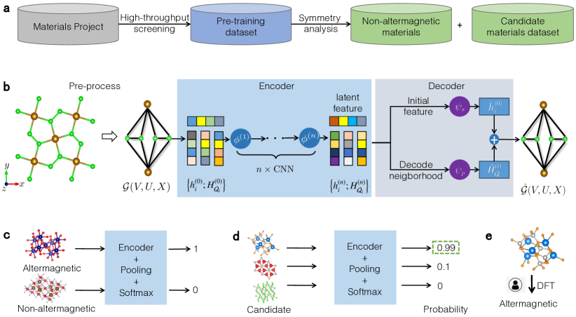
Figure 1: Workflow of the pre-trained model for searching altermagnetic materials. a, Construction of candidate material datasets using high-throughput screening and symmetry analysis. b, The pre-training autoencoder framework for crystal materials. The input of the model is the crystal structure. Each crystal structure can be represented as a multi-edge graph neural network (GNN). The encoder is built by the graph convolutional neural network. The decoder is built on the Waterstein neighborhood reconstruction. c, The fine-tuning procedure with loading pre-training stage weight matrix. d, The prediction procedure by inputting candidate materials. e, Validation of the altermagnetic property via the first principle electronic structure calculations.

Of 91,649 total candidates, we discovered 25 new altermagnetic materials covering metals, semiconductors, and insulators, based on only 14 positive samples. The wide range of electronic structural properties implies that various novel physical properties appear in these newly discovered altermagnetic materials, e.g., anomalous Hall effect, anomalous Kerr effect, and topological property, as demonstrated in theoretical analyses. It is also worth noting that we discovered 8 $i$-wave altermagnetic materials for the first time, essentially filling in the gap in the literature. We conclude that the AI search engine performs much better than human experts and suggests a set of new altermagnetic materials with unique properties, outlining its potential for accelerated discovery of the materials with targeting properties. We also discuss the pathway of developing pre-trained graph models for the discovery of other types of materials.

Results

Dataset screening based on symmetry analysis

Our goal is to screen altermagnetic materials from the Material Project [27], which contains 154,718 crystal materials. Since this material database includes both magnetic and non-magnetic materials, we first filtered out materials containing magnetic atoms. In this work, we considered materials with 3d transition metals or 4f rare earth elements. After filtering and de-duplication, we obtained 91,649 potential magnetic materials. Due to the complexity of the magnetic properties of materials with multiple magnetic atoms, we further excluded such materials, resulting in 68,116 potential magnetic materials, which constitute the pre-training dataset.

Altermagnetism is characterized by compensated antiparallel spin sublattices connected by the spin symmetry $\{C_{2}^{\perp}||R_{i}\}$ transformation but not connected by the spin symmetry $\{T||IT\}$ or $\{C_{2}^{\perp}||\tau\}$ transformation. Since the space groups $P1(1)$ and $P\bar{1}(2)$ do not have $R_{i}$ symmetry, all materials with space groups $P1$ and $P\bar{1}$ symmetry are excluded from the pre-training dataset. If collinear antiferromagnets have type-IV magnetic space group symmetry, their compensated antiparallel spin sublattices must be connected by the spin symmetry $\{C_{2}^{\perp}||\tau\}$ transformation in a nonrelativistic case. So all collinear antiferromagnetic materials with type-IV magnetic space group symmetry are conventional antiferromagnets but not altermagnets. Different from antiferromagnetic materials with the type-IV magnetic space group symmetry, the magnetic cell and crystal cell of materials with type-III magnetic space group symmetry are usually the same, which leads to these materials without the spin symmetry $\{C_{2}^{\perp}||\tau\}$. If the magnetic cell of a collinear antiferromagnet is a supercell whereas its spin arrangement breaks the spin symmetry $\{C_{2}^{\perp}||\tau\}$, then the collinear antiferromagnet may be a supercell altermagnet [16]. Although there exist 4 known supercell altermagnetic materials, we do not consider this situation and exclude them in the positive samples. Since compensated antiparallel spin sublattices in altermagnets require that the candidate magnetic materials have an even number of magnetic atoms in their crystal primitive cell, we first ruled out 18,546 magnetic materials with the odd number of magnetic atoms in the primitive crystal cell from the pre-training dataset.

Furthermore, magnetic materials with type-III magnetic space group symmetry can be divided into two classes according to space-inversion symmetry. If a collinear antiferromagnet has no space-inversion symmetry, the collinear antiferromagnet must be an altermagnetic material. For collinear antiferromagnetic materials with space-inversion symmetry, if these collinear antiferromagnetic materials have only a pair of spin antiparallel magnetic atoms in primitive crystal cells that are not located at invariant space-inversion points, the pair of spin antiparallel magnetic atoms must be connected by the spin symmetry $\{T||IT\}$. That is to say, these collinear antiferromagnets are non-altermagnetic materials (7,045 in total). Therefore, based on symmetry analysis, we screened out 25,591 non-altermagnetic materials. These materials, along with the known 14 altermagnetic materials (e.g., as positive samples), together constitute the fine-tuning dataset. By removing the 25,591 non-altermagnetic materials from the pre-training dataset, we obtained the candidate dataset (42,525 materials). The aforementioned screening process is depicted in Extended Data Fig. 1. In the following, we train a neural network to screen and predict altermagnetic materials from the candidate dataset.

Pre-training GNN for materials discovery

Conventional approaches for discovering materials with altermagnetic properties heavily rely on experts’ physical intuition and perform trial-and-error verification of the properties for each material through the first-principles electronic calculations, which are time-consuming and not scalable for screening crystal materials in a large search space. Although AI methods have shown great potential for material screening and discovery, there still remain numerous challenges in the field of discovering altermagnetic materials that have not yet been accommodated in existing research practices. In particular, training a reliable predictive model under the condition of very limited labels is intractable, e.g., the number of known altermagnetic materials, as positive samples (training labels), is extremely limited (only 14 altermagnetic materials [2]). We address this challenge by introducing a pre-training technique, which was first proposed in the natural language processing field [28], and subsequently demonstrated with remarkable capabilities for computer vision [29] and bioinformatics [30].

As detailed in the symmetry analysis above, we first construct the pre-training dataset and candidate materials dataset based on high-throughput screening and symmetry analysis (see Fig 1a). The model is based on a pre-trained GNN that leverages material crystal structure information to predict altermagnetic materials [22], consisting of a graph convolutional network encoder, and a decoder that reconstructs graph features based on the optimal transport theory [31]. Fig 1b depicts the schematic of the network, with the detailed architecture shown in Extend Data Fig 2. The process of inputting crystal structures into the model begins with a pre-processing stage, where the crystal structure information is transformed into a graph representation. Then, we pre-train the model based on the pre-training dataset which contains 68,116 materials, and then fine-tune the pre-trained model based on the fine-tuning dataset (14 altermagnetic materials plus 25,591 non-altermagnetic materials) (see Fig 1c). During the fine-tuning, we utilize the pre-trained encoder and employ up-sampling techniques (duplication and rotation) to balance the number of positive and negative samples for a binary classification task. Afterward, we can obtain the classifier model, which is then used to screen the altermagnetic materials (Fig 1d). All possible candidate crystal structures (42,525) are input into the classifier model for prediction. The model provides a probability estimate for each sample, and we selected the material with a probability greater than 0.9 as the candidate material. Next, we utilize the first principle electronic structure calculations (Fig 1e) to verify whether the candidates are altermagnetic materials. Furthermore, once the new altermagnetic materials are verified and confirmed, we added the new one to the fine-tuning dataset and then re-perform the fine-tuning and prediction iteratively. Through three rounds of iteration and leveraging information from only 14 known altermagnetic materials, we identified 25 new altermagnetic materials. The details of the proposed architecture are shown in Extended Data Fig. 2. The additional information for the pre-trained model can be found in Supplementary Note A.

To demonstrate the capability of our pre-trained crystal material model, we fed all the candidate materials in batches into the pre-trained encoder which provides a corresponding latent space vector for each material. We utilized principal component analysis (PCA) for dimensionality reduction and performed feature visualization and t-SNE visualization on the latent space vectors (see Extended Data Fig. 3). The results show that the data in the candidate set have a clear clustering phenomenon after pre-training, which indicates that the pre-training process can group materials containing similar information together.

Table 1: Discovered 25 new altermagnetic materials verified by electronic structure calculations. We further give the nonmagnetic space group, even-parity wave anisotropy, metal (M) and insulator (I) conduction type. The altermagnetic $NdB_{2}C_{2}$ is confirmed by previous neutron scattering experiments [32] and our symmetry analysis. “NA” indicates that this material has not been experimentally synthesized.

Number	Materials	Space group	Anisotropy	Conduction	References
1	$Nb_{2}FeB_{2}$	$P4-mbm\leavevmode\nobreak\ (127)$	$g$-wave	M	[33]
2	$Ta_{2}FeB_{2}$	$P4-mbm\leavevmode\nobreak\ (127)$	$g$-wave	M	[34]
3	$NdB_{2}C_{2}$	$P4-mbm\leavevmode\nobreak\ (127)$	$g$-wave	M	[32]
4	$Mg_{2}FeIr_{5}B_{2}$	$P4-mbm\leavevmode\nobreak\ (127)$	$g$-wave	M	[35]
5	$Mg_{2}MnIr_{5}B_{2}$	$P4-mbm\leavevmode\nobreak\ (127)$	$g$-wave	M	[35]
6	$Mg_{2}NiIr_{5}B_{2}$	$P4-mbm\leavevmode\nobreak\ (127)$	$g$-wave	M	[35]
7	$Sc_{2}VIr_{5}B_{2}$	$P4-mbm\leavevmode\nobreak\ (127)$	$g$-wave	M	[36]
8	$Sc_{2}MnIr_{5}B_{2}$	$P4-mbm\leavevmode\nobreak\ (127)$	$g$-wave	M	[36]
9	$CaLaFeAgO_{6}$	$Pc\leavevmode\nobreak\ (7)$	$d$-wave	M	NA
10	$CaLaCr_{2}O_{6}$	$Pmn21\leavevmode\nobreak\ (31)$	$d$-wave	M	NA
11	$NiF_{3}$	$R-3C\leavevmode\nobreak\ (167)$	$i$-wave	M	[37]
12	$FeHO_{2}$	$Pmn21\leavevmode\nobreak\ (31)$	$d$-wave	I	[38]
13	$NaFeO_{2}$	$Pna2_{1}\leavevmode\nobreak\ (33)$	$d$-wave	I	[39]
14	$NaFeO_{2}$	$P-4_{1}2_{1}2\leavevmode\nobreak\ (92)$	$d$-wave	I	[40]
15	$MnO_{2}$	$Pnma\leavevmode\nobreak\ (62)$	$d$-wave	I	[41]
16	$MnO_{2}$	$I4/m\leavevmode\nobreak\ (87)$	$d$-wave	I	[42]
17	$Ca_{3}Cr_{2}O_{7}$	$Cmc2_{1}\leavevmode\nobreak\ (36)$	$d$-wave	I	NA
18	$ZrCrO_{3}$	$Pnma\leavevmode\nobreak\ (62)$	$d$-wave	I	NA
19	$ZrMnO_{3}$	$R3c\leavevmode\nobreak\ (161)$	$i$-wave	I	NA
20	$VF_{3}$	$R-3C\leavevmode\nobreak\ (167)$	$i$-wave	I	[37]
21	$CrF_{3}$	$R-3C\leavevmode\nobreak\ (167)$	$i$-wave	I	[37]
22	$FeF_{3}$	$R-3C\leavevmode\nobreak\ (167)$	$i$-wave	I	[37]
23	$CoF_{3}$	$R-3C\leavevmode\nobreak\ (167)$	$i$-wave	I	[37]
24	$MnO$	$P6_{3}mc\leavevmode\nobreak\ (186)$	$i$-wave	I	[43]
25	$CaMnN_{2}$	$P6_{3}-mmc\leavevmode\nobreak\ (194)$	$i$-wave	I	NA

Discovered altermagnetic materials

Based on the proposed AI search engine, we successfully discovered 25 new altermagnetic materials including 11 metals and 14 insulators (see Table 1). The computational results for most of the newly discovered altermagnetic materials are shown in the Supplementary Note B and Supplementary Figs. S.3–S.13. Moreover, the $d$-wave, $g$-wave, and $i$-wave altermagnets can be found in the predicted 25 altermagnetic materials as shown in Table 1. In particular, we predicted 8 $i$-wave altermagnetic materials for the first time. The $i$-wave altermagnetic $MnO$ is shown as an example in the Extended Data Fig. 4.

The 11 metallic altermagnetic materials can be divided into two classes according to whether the integral of the Berry curvature of the occupied states over the Brillouin zone is zero, which depends on the symmetry of the altermagnetic materials. By analysis of the magnetic point group symmetry, the 8 metallic altermagnetic materials ($Nb_{2}FeB_{2}$, $Ta_{2}FeB_{2}$, $Mg_{2}FeIr_{5}B_{2}$, $Mg_{2}MnIr_{5}B_{2}$, $Sc_{2}VIr_{5}B_{2}$, $CaLaFeAgO_{6}$, $CaFe_{2}O_{5}$, and $NiF_{3}$) have nonzero Berry curvature for the integral of the occupied states over the Brillouin zone, implying that odd-under-time-reversal responses (e.g., anomalous Hall and Kerr effects) can be realized in these materials. Especially, the calculated intrinsic anomalous Hall conductance of altermagnet $Nb_{2}FeB_{2}$ is $-100\Omega^{-1}cm^{-1}$ [44], which is the same order of magnitude as those of ferromagnetic metals. Since the remaining 3 altermagnetic materials ($NdB_{2}C_{2}$, $Sc_{2}MnIr_{5}B_{2}$, $Mg_{2}NiIr_{5}B_{2}$) have zero Berry curvature for the integral of the occupied states over the Brillouin zone, odd-under-time-reversal responses are not observed. Interestingly, the metallic altermagnet $NdB_{2}C_{2}$ has odd-under-time-reversal Dirac fermions (see Extend Data Fig. 5b), but $Sc_{2}MnIr_{5}B_{2}$ and $Mg_{2}NiIr_{5}B_{2}$ have odd-under-time-reversal sixfold degenerate fermions (see Extend Data Fig. 5e and h) on the $\rm{\Gamma-Z}$ around the Fermi level, which is protected by the spin point group symmetry. When considering spin-orbit coupling (SOC), the 3 metallic altermagnets $NdB_{2}C_{2}$, $Sc_{2}MnIr_{5}B_{2}$, and $Mg_{2}NiIr_{5}B_{2}$ have $D_{4h}$ point group symmetry which must be broken in ferromagnets, and the $C_{4v}$ double point group symmetry protects the odd-under-time-reversal Dirac fermions of the metallic altermagnets $Sc_{2}MnIr_{5}B_{2}$ and $Mg_{2}NiIr_{5}B_{2}$ on the $\rm{\Gamma-Z}$ (see Extend Data Fig. 5f and i). Moreover, the pair odd-under-time-reversal Dirac points in $Mg_{2}NiIr_{5}B_{2}$ are very close to the Fermi level, which is an advantage for investigating its novel physical properties in experiments.

On the other hand, ferromagnetic semiconductors that have spintronic and transistor functionalities could be applied to the next generation of electronic devices. However, the ferromagnets usually are metals with a high Curie temperature and hold no brief for insulators with a high Curie temperature. Altermagnets with compensated antiparallel sublattices not only are in favor of insulators with a high Neel temperature but also have spintronic and transistor functionalities [2]. Thus, altermagnets open a new pathway to bypass the difficulties of ferromagnets. Here, we employed the LDA+U method [45] to predict 9 altermagnetic semiconductors  Supplementary Table S.2. Furthermore, the altermagnetic $FeHO_{2}$ may have a spin-triplet excitonic phase. From Extend Data Fig. 6i, we observe that there is large spin splitting on the $\rm{T-\Gamma-T}$ directions and the spin of valence and conduction band are opposite, which may result in the spin-triplet excitonic phase [46]. Moreover, the energy of altermagnetic state (AFM1) is much lower than that of the other three magnetic states (see Extend Data Fig. 6g), indicating that $FeHO_{2}$ may have a Neel temperature above the room temperature. Thus, the altermagnetic $FeHO_{2}$ is a very interesting material that, we believe, will attract both theoretical and experimental interests. In the following, we present in detail two altermagnetic materials which are metal and semiconductor, respectively.

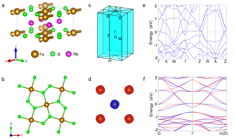
Figure 2: The crystal and electronic structure of the altermagnetic $Nb_{2}FeB_{2}$. a, The side view of altermagnetic $Nb_{2}FeB_{2}$. b, The top view of altermagnetic $Nb_{2}FeB_{2}$. c, The Brillouin zone (BZ) with high-symmetry points of altermagnetic $Nb_{2}FeB_{2}$. The cyan plane represents the nodal surface of BZ. The m represents the mirror symmetry $M_{y}$. d, The anisotropic spin-charge density deriving from an anisotropic crystal field. e, The electronic band structure along high-symmetry directions without spin-orbit coupling (SOC). f, The electronic band structure along non-high-symmetry directions without SOC. The red and blue lines represent the spin-up and spin-down energy bands, respectively. The electronic structure is calculated under correlation interaction $\rm{U=4.82\leavevmode\nobreak\ eV}$.

$Nb_{2}FeB_{2}$ has space group $P4-mbm\leavevmode\nobreak\ (127)$ symmetry, and the corresponding elementary symmetry operations are $C_{4z}$,$C_{2x}(\frac{1}{2},\frac{1}{2})$ and $I$, which yield the point group $D_{4h}$. The crystal structure of $Nb_{2}FeB_{2}$ is composed of $Fe-B$ atoms layer and $Nb$ atoms layer as shown in Fig. 2a. Moreover, the two $Fe$ atoms in the primitive cell are surrounded by two $B$ atomic quadrilaterals with different orientations, respectively (Fig. 2b). Very recentlly, $Nb_{2}FeB_{2}$ has been predicted to be a Neel antiferromagnet, which is shown in Fig. 2a. Due to the anisotropic $Fe-B$ quadrilateral, the spin-charge density of $Fe$ atoms is anisotropic (see Fig. 2d). Thus, compensated antiparallel spins are not connected by the spin symmetry $\{T||IT\}$ or $\{C_{2}^{\perp}||\tau\}$ but are connected by the spin symmetry$\{C_{2}^{\perp}||C_{2x}(\frac{1}{2},\frac{1}{2})\}$; that is to say, $Nb_{2}FeB_{2}$ is an altermagnetic material. The spin symmetry $\{C_{2}^{\perp}||M_{x}(\frac{1}{2},\frac{1}{2})\}$ protects the spin degeneracy in electronic bands on the $k_{x}=0$ and $\pi$ planes, considering the spin symmetries $\{E||C_{4z}\}$, the altermagnetic $Nb_{2}FeB_{2}$ has six node surfaces in the Brillouin zone (see Fig. 2c). Thus, $Nb_{2}FeB_{2}$ is a $g$-wave altermagnet described by the non-trivial spin Laue group $P^{1}4-^{1}m^{2}m^{2}m$. Fig. 2e shows that the electronic bands of the altermagnetic $Nb_{2}FeB_{2}$ are spin degenerate along the high-symmetry directions, which is consistent with our symmetry analysis. As can be seen from the Fig. 2f, all the bands are spin-splitting and spin antisymmetric in the non-high-symmetry $D-\Gamma-m(D)$ direction, which reflects the characteristics of $g$-wave spin polarization. On the other hand, the valence bands and the conduction bands have multiple crossing points on the high-symmetry and non-high-symmetry directions, such as the $\Gamma-X$ and $\Gamma-D$ directions, indicating that the altermagnet $Nb_{2}FeB_{2}$ is a topologically nontrivial metal. When considering SOC, the easy magnetization axis of altermagnet $Nb_{2}FeB_{2}$ is along the $x$ direction. Accordingly, the altermagnet $Nb_{2}FeB_{2}$ has $C_{2z}T,C_{2x}(\frac{1}{2},\frac{1}{2})T,C_{2y}(\frac{1}{2},\frac{1}{2})T,I,M_{z}T,M_{x}(\frac{1}{2},\frac{1}{2})T,M_{y}$ point symmetries, which make the anomalous Hall conductance both $\sigma_{xy}$ and $\sigma_{yz}$ zero, but $\sigma_{xz}$ non-zero, which has been predicted by our previous theoretical study [44]. Likewise, the anomalous Kerr effects can also be realized in the altermagnet $Nb_{2}FeB_{2}$.

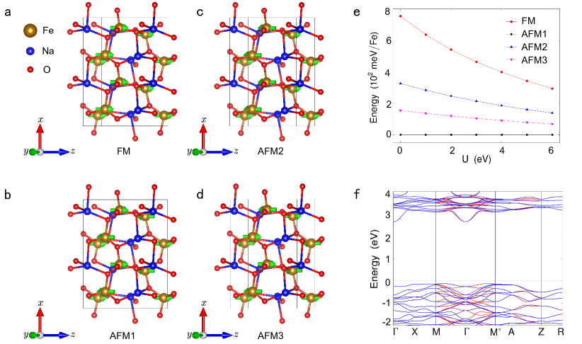
Figure 3: The crystal and electronic structure of the altermagnetic $NaFeO_{2}\leavevmode\nobreak\ (92)$. a, The crystal structures of the $NaFeO_{2}\leavevmode\nobreak\ (92)$ with FM structures. b, The crystal structures of the $NaFeO_{2}\leavevmode\nobreak\ (92)$ with AFM1 structures. c, The crystal structures of the $NaFeO_{2}\leavevmode\nobreak\ (92)$ with AFM2 structures. d, The crystal structures of the $NaFeO_{2}\leavevmode\nobreak\ (92)$ with AFM3 structures. e, Relative energy of different magnetic states with the variation of correlation interaction $U$. f, The electronic band structure of $NaFeO_{2}(92)$ along high-symmetry directions without SOC. The red and blue lines represent the spin-up and spin-down energy bands, respectively. The electronic structure is calculated under correlation interaction $\rm{U=4\leavevmode\nobreak\ eV}$.

The other altermagnetic material that we would like to mention is $NaFeO_{2}$. The crystal structure of $NaFeO_{2}$ is shown in Fig. 3a-d with space group $P-4_{1}2_{1}2\leavevmode\nobreak\ (92)$ symmetry. The corresponding elementary symmetry operations are $C_{4z}(\frac{1}{2},\frac{1}{2},\frac{1}{4})$ and $C_{2x}(\frac{1}{2},\frac{1}{2},\frac{3}{4})$, which yield the point group $D_{4}$. Since the $d$ orbitals of $Fe$ are half occupied and the angle between $Fe-O-Fe$ is 136 degrees in $NaFeO_{2}$, the superexchange interactions result in the nearest neighbor $Fe$ ions with opposite magnetic moments and the next neighbor $Fe$ ions with the same magnetic moments. Hence, the magnetic ground state of $NaFeO_{2}$ will be the AFM1 (see Fig. 3b). To verify our theoretical analysis, we consider four different magnetic structures, which are shown in Figs. 3a-d. It can be seen that the magnetic structure AFM1 is always in the ground state of $NaFeO_{2}$ under different correlation interactions $U$ (see Fig. 3e). Moreover, the energy of the AFM1 state is much lower than that of the other three magnetic states (Fig. 3e), implying that $NaFeO_{2}$ may have a Neel temperature above the room temperature. It is shown in Fig. 3b that the magnetic and crystal primitive cells of $NaFeO_{2}$ are the same, which break $\{C_{2}^{\perp}||\tau\}$ spin symmetry. Thus, $NaFeO_{2}$ is an altermagnetic material due to the lack of space-inversion symmetry.

We also calculated the electronic band structure along the high-symmetry directions. Fig. 3f shows that the altermagnet $NaFeO_{2}$ is a semiconductor with a band gap of 2.75 eV. The spin-degenerate bands on the $\Gamma-{\rm{X,\leavevmode\nobreak\ M}}^{*}-{\rm{A}}$ and $\rm{Z-R}$ directions (the $\rm{X-M}$ direction) are protected by the spin symmetry $\{C_{2}^{\perp}||C_{2y}(\frac{1}{2},\frac{1}{2},\frac{1}{4})\}$ ( $\{C_{2}^{\perp}||C_{2y}(\frac{1}{2},\frac{1}{2},\frac{3}{4})\}$) (see Fig. 3f). In fact, the spin symmetry $\{T||C_{2y}T(\frac{1}{2},\frac{1}{2},\frac{1}{4})\}$ ( $\{T||C_{2x}T(\frac{1}{2},\frac{1}{2},\frac{3}{4})\}$) can protect spin degeneracy of bands on the $k_{y}=0$ and $\pi$ (the $k_{x}=0$ and $\pi$) planes. That is to say, the altermagnet $NaFeO_{2}$ has four nodal surfaces in the Brillouin Zone. Thus, $NaFeO_{2}$ is a $d$-wave altermagnet which is reflected by the spin-splitting bands on the $\rm{M}-\Gamma-\rm{M}^{*}$ directions. Considering the $d$-wave altermagnets allowing unique spin current by electrical means [4], the altermagnet $NaFeO_{2}$ may have both spintronic and transistor functionalities at the room temperature.

Discussion

AI approaches have shown ground-breaking capabilities in the discovery of materials in a large search space. An intractable challenge faced by AI lies in the shortage of sufficient labels or positive samples, e.g., in the case of the discovery of altermagnetic materials. We herein introduced an AI search engine that combines pre-trained crystal models (GNN pre-training and optimal transport theory) and physics-based methods (symmetry analysis and first-principles electronic structure calculations) to discover new altermagnetic materials with specific properties under highly limited labeled sample conditions. Among 91,649 possible candidates, we identified 25 new altermagnetic materials covering metal, semiconductor, and insulator, based on only 14 positive samples. We observed various novel physical properties in these newly discovered altermagnetic materials, e.g., anomalous Hall effect, anomalous Kerr effect, and topological property. It is noted that 8 out of these 25 altermagnetic materials are $i$-wave types, which are discovered for the first time essentially filling a gap in the literature. We demonstrate that the AI search engine is capable of uncovering a set of altermagnetic materials with unique properties, highlighting its potential for accelerated discovery of the materials with targeting properties.

There still remain some potential limitations associated with the AI search engine. Firstly, we have to admit that the issue of imbalance between positive and negative samples during the fine-tuning stage exists, primarily due to the scarcity of known positive samples. Utilizing the translational and rotational symmetries of crystals to augment positive sample data may help address this challenge, which will be demonstrated in our future work. Another limitation is that we have not yet found ideal altermagnetic topological insulators and altermagnetic topological semimetals (such as odd-under-time-reversal Dirac, and sixfold semimetals). Employing the decoder based on the pre-trained model to generate potential altermagnetic materials holds promise in overcoming this challenge. Furthermore, adopting a multimodal pre-training approach offers the potential to further enhance the accuracy of model predictions. The current pre-training only considers the single modality of crystal structure information. Leveraging information from other modalities (such as textual descriptions of crystal structures) may enhance the performance of the pre-trained model. These methods will be further explored in our future research endeavors.

Compared to conventional methods, this AI search engine significantly improves the efficiency of altermagnetic materials discovery. The success of this engine lies not only in its predictive capabilities but also in its ability to leverage extensive crystal structure data and deep learning techniques, allowing for pre-training without explicit reference to underlying physical laws, to reveal complex correlations and patterns in new materials. This effort may present new opportunities in the field of material discovery across different disciplines.

Methods

We herein introduce the model details and implementation specifics.

Model details

Architecture overview.

The concept of pre-training a large deep learning model and subsequently applying it to perform downstream tasks originally originated in the field of natural language processing (NLP). Large-scale NLP models, such as GPT [47], and their derivatives, employ transformers as text encoders. These encoders transform input texts into embeddings and establish pre-training objectives based on these embeddings, including generative loss and masked language modeling loss. The pre-training process is typically unsupervised, based on large-scale unlabeled samples. In contrast to traditional end-to-end neural network models, pre-trained models can achieve excellent performance even with limited labeled positive samples. We thus consider utilizing the pre-training technique to fully leverage the information from existing crystal materials databases and treat the discovery of altermagnetic materials as a downstream task.

The objective of our proposed pre-training model for crystal materials is to learn the information embedded within crystal structures. To enhance the learning capacity of the pre-training model, we proposed a graph auto-encoder architecture (see Fig. 1 and Extended Data Fig. 2). The encoder consists of $n$ layers of graph convolution to learn crystal embeddings, while the decoder employs the Wasserstein distance based on the optimal transport theory [25] for the reconstruction of the input crystal structures. Specifically, the encoder aims to encode the graphical representation of crystal materials into a high-dimensional matrix, while the goal of the decoder is to decode this one back into the graphical representation of crystal materials. Through extensive training with unlabeled data, the model effectively converges (as depicted in the pre-training loss history as shown in Supplementary Fig. S.1). We believe that the pre-trained encoder can effectively project the crystal structures into crystal embeddings. Leveraging the encoder of the pre-trained model, we built the classifier model by incorporating a pooling layer and a softmax function. Subsequently, we trained the classifier model using the fine-tuning dataset. This trained model is then employed to screen the candidate materials, offering the probability of whether the target material is altermagnetic. The hyperparameters of the model were obtained by grid search, as listed in Supplementary Table S.1. In summary, our model comprises four main components: crystal data pre-processing, an encoder constructed using graph convolutional neural networks, a decoder built based on optimal transport theory, and the construction of a classifier model. We elaborate on each of these components one by one as follows.

Crystal data pre-processing.

The data pre-processing procedure aims to bridge the crystal structure and the crystal graph representation [22]. The input of the model is a crystal structure file (.cif) that contains three primitive translation vectors of the primitive unit cell and the positional information of each atom. It satisfies the organization invariance for atomic indexing and the size invariance for unit cell selection. We define the graph representation $\mathcal{G}(V,U,X)$ to describe the crystal structure information, where $V$ denotes the set of nodes, $U$ the set of edges, and $X$ the set of features. First, we represent atoms as nodes $v_{i}$ in a crystal graph representation, where $i=1,...,|V|$. Since periodic boundary conditions are taken into consideration, equivalent nodes are merged to obtain irreducible nodes. Then, for each node $v_{i}$, we consider the neighborhood nodes $v_{j}$, where $j=,1,...,|\mathcal{N}_{i}|$ and $\mathcal{N}_{i}$ the set of neighborhood nodes for $v_{i}$. The $k$ connections between nodes $v_{i}$ and $v_{j}$ are denoted as the edge $u_{(i,j)_{k}}$ in the graph. Next, the initial node features $\big{\{}h_{i}^{(0)}\big{\}}_{i=1}^{|V|}$ are given through one-hot encoding based on the sequence of atoms in the crystal structure. We use $H_{\mathcal{N}_{i}}^{(0)}$ to denote the neighbor node features of node $v_{i}$. Here, $v_{i}$ denotes the $i$-th node. Each edge $u_{(i,j)_{k}}\in U$ is represented by a feature vector $u_{(i,j)_{k}}$ that corresponds to the $k$-th bond linking node $v_{i}$ and node $v_{j}$. A feature vector $h_{i}\in X$ encoding the attribute of the atom corresponding to node $v_{i}\in V$ is used to represent each node $v_{i}$. An example for determining the atom connectivity is illustrated in Supplementary Fig. S.2.

Crystal graph convolutional encoder.

The encoder is used to represent the input crystal structure information as a high-dimensional matrix (Extended Data Fig. 2$\bf{c}$), which contains $n$ convolutional layers. The $t$-th convolutional layer updates the node feature vector $h_{i}^{(t)}$ via convolution function $h_{i}^{(t+1)}={\rm{Conv}}\big{(}h_{i}^{(t)},h_{j}^{(t)},u_{(i,j)_{k}}\big{)}$. We denote the graph convolution function with $g$, which iteratively updates the overall feature vector $h_{i}$, whose output is the input for the next step. The node index in feature vector $h_{i}$ and length of $h_{i}$ are invariant for every step, We construct the first concatenate neighbor vector as $z^{(t)}_{(i,j)_{k}}=h^{(t)}_{i}\oplus h^{(t)}_{j}\oplus u_{(i,j)_{k}}$ in step $t$, and then perform the convolution operation to update the feature as follows:

$$h_{i}^{(t+1)}=h_{i}^{(t)}+\sum_{v_{j}\in\mathcal{N}_{i},v_{m}\in\mathcal{M}_{i},k}\sigma\left(z^{(t)}_{(i,j)_{k}}W_{f}^{(t)}+b_{f}^{(t)}\right)\odot g\left(z^{(t)}_{(i,j)_{k}}W_{s}^{(t)}+h_{i,m}^{(t)}W_{m}^{(t)}+b_{s}^{(t)}\right),$$ (1)

where $\odot$ denotes the element-wise multiplication, $\mathcal{M}_{i}$ the magnetic atoms corresponding to node $v_{i}$, and $\sigma$ the sigmoid activation function. Since the magnetic atoms are important for the material to exhibit altermagetic properties, we added the weight term $W_{m}^{(t)}$ for the magnetic atoms. The weight function $W_{c}^{(t)},W_{s}^{(t)},W_{m}^{(t)}$ are the convolution weight matrix, self-weight matrix, and magnetic atom weight matrix of the $t$-th layer, respectively. In Eq. (1), we incorporate the residual term $h_{i}^{(t)}$ to enhance the training of the neural network.

Neighborhood wasserstein reconstruction decoder.

The decoder (denoted by $\psi$) is utilized to restore the input graph representation of a crystal from the crystal embeddings, which mainly consists of two parts (see Extended Data Fig. 2a), one for node feature reconstruction (denoted by $\psi_{s}$) and the other for adjacent node feature reconstruction (denoted by $\psi_{p}$), namely, $\psi=(\psi_{p}+\psi_{s})$. Here, $\psi_{s}={\rm{MLP}}_{s}\big{(}h_{i}^{(t)}\big{)}$ is used to reconstruct the node features, where MLP indicates a multilayer perception. The architecture of the decoder block, as shown in Extended Data Fig. 2b, follows the design in [31].

In particular, we adopt the $n$-hop neighboring Wasserstein decoder for graph feature reconstruction. We can obtain $\big{\{}h_{i}^{(0)},H_{\mathcal{N}_{i}}^{(0)}\big{\}}$ from the pre-processing procedure. For each node $v_{i}\in V$, we update the node representation $h_{i}^{(t+1)}$ via the GNN layer in the encoder, which gathers information from $h_{i}^{(t)}$ and its neighbor representations $H_{\mathcal{N}_{i}}^{(t)}$, namely, $h_{i}^{(t+1)}=\phi^{(t)}\big{(}h_{i}^{(t)},H_{\mathcal{N}_{i}}^{(t)}\big{)}$. Note that the neighborhood set of node features $H_{\mathcal{N}_{i}}^{(t)}$ can be directly assembled based on the node adjacency. Consequently, we solve the following optimization problem to train the network:

$$\arg\min_{\phi,\psi}\sum_{v_{i}\in V}\mathcal{L}\left(h_{i}^{(t)},H_{\mathcal{N}_{i}}^{(t)},\psi\left(h_{i}^{(t+1)},H_{\mathcal{N}_{i}}^{(t+1)}\right)\right),$$ (2)

where $\mathcal{L}(\cdot,\cdot)$ denotes the reconstruction loss over $0\leq t<n$. The loss function $\mathcal{L}$ can be decomposed into two distinct elements, each gauging the reconstruction of self and neighborhood node features, respectively, written as

$$\mathcal{L}=\lambda_{s}\mathcal{L}_{s}\left(h_{i}^{(0)},\psi_{s}\left(h_{i}^{(n)}\right)\right)+\lambda_{p}\sum_{t=0}^{n-1}\mathcal{L}_{p}\left(H^{(t)}_{Q_{i}},\hat{H}^{(t)}_{Q_{i}}\right),$$ (3)

where $\hat{H}^{(t)}_{Q_{i}}=\psi_{p}^{(t+1)}\Big{(}h_{i}^{(t+1)},H_{\mathcal{N}_{i}}^{(t+1)}\Big{)}$ denotes the reconstructed neighborhood set of node features based on the sampling network shown in Extended Data Fig. 2b. Here, $Q_{i}\subset\mathcal{N}_{i}$ denotes the set of $q$ samples of neighborhood nodes for $v_{i}$; $\lambda_{s}$ and $\lambda_{p}$ are the weighting coefficients; and $\mathcal{L}_{s}$ stands for the reconstruction error of the node features, given by

$$\mathcal{L}_{s}\left(h_{i}^{(0)},\psi_{s}\left(h_{i}^{(n)}\right)\right)=\left\|h_{i}^{(0)}-\psi_{s}\left(h_{i}^{(n)}\right)\right\|^{2}_{2}.$$ (4)

In Eq. (3), $\mathcal{L}_{p}$ is the loss function used to measure the reconstruction of the neighborhood set of node features $H^{(t)}_{Q_{i}}$. Inspired by [31], we evaluate this loss function by a Monte Carlo method. Specifically, for node $v_{i}$, the distribution of its neighborhood information can be empirically represented by $\mathcal{P}^{(t)}_{i}$ defined as follows:

$$\mathcal{P}^{(t)}_{i}=\sum_{v_{j}\in\mathcal{N}_{i}}\delta_{h_{j}}^{(t)},$$ (5)

where $\delta_{h_{j}}^{(t)}$ denotes the Dirac delta function. Here, we adopt the 2-Wasserstein distance, which measures the similarity between two distributions, to construct the loss [31], expressed as

$$\mathcal{L}_{p}\left(H_{\mathcal{N}_{i}}^{(t)},\hat{H}^{(t)}_{Q_{i}}\right)=\mathcal{W}_{2}^{2}\left(\mathcal{P}^{(t)}_{i},\hat{H}^{(t)}_{Q_{i}}\right).$$ (6)

In our experiments, we fix $q=10$ based on a Hungarian matching, which avoids heavy computational overhead meanwhile retaining accuracy, when evaluating Eq. (6) during training.

Classifier model.

The classifier model is constructed by adding a pooling layer and a softmax module after the encoder of the pre-trained model (see Extended Data Fig. 2c). The pooling layer is applied to the embedding of the pre-trained encoder to generate an overall feature vector $h_{g}$ that can be represented by a pooling function given by $h_{g}={\rm{Pool}}(h_{0}^{(0)},h_{1}^{(0)},...h_{N}^{(0)},\dots,h_{N}^{(n)})$, where $n$ is the number of convolution layer and $N$ is the number of nodes in graph. The softmax module in the classifier model ensures that the output for each candidate material through the model is a probability in the range of $[0,1]$, representing the likelihood of the candidate material being an altermagnetic material.

Implementation details

The pre-training model.

To extract the crystal embeddings of the candidate materials, we employ a graph convolution neural network as an encoder, which consists of 3 graph convolution layers. For classification, we utilize a pooling layer and a multilayer perceptron as the projection head, comprising two fully connected layers with a ReLU activation layer and a Dropout layer. In terms of optimization, we use the Adam optimizer with a learning rate of 0.001. Additionally, we implement MultiStepLR with milestones set at 100. To ensure stability during training, we train our classifier model with a dropout rate of 0.25. This is done using a batch size of 512 and training over 500 epochs on 2 NVIDIA A100 GPUs. We then label these materials whose probabilities exceed 0.9 as potential altermagnetic candidates in all experiments. To train and evaluate our model efficiently, we leverage the distributed deep learning framework Accelerate. More details of the model training are discussed in Supplementary Note A. Given this specific network architecture, we can complete the training and evaluation process of the classifier model in less than 1.5 hours on our datasets. This significantly improves the overall efficiency of our workflow.

The first-principles electronic calculation.

The first-principles electronic structure calculations were performed in the framework of density functional theory (DFT) using the Vienna Abinitio Simulation Package (VASP) [48]. The generalized gradient approximation (GGA) of the Perdew-BurkeErnzerhof (PBE) type was adopted for the exchange-correlation functional [49]. The projector augmented wave (PAW) method was employed to describe the interactions between valence electrons and nuclei [50]. To account for the correlation effects of 3d and 4f orbitals, we performed $\rm GGA+U$ calculations by using the simplified rotationally invariant version introduced by Dudarev et al. [45].

Data availability

The crystal data are available from the Materials Project database via the web interface at https://materialsproject.org or the API at https://api.materialsproject.org.

Code availability

All the source codes to reproduce the results in this study are available on GitHub at https://github.com/zfgao66/MatAltMag. We rely on PyTorch (https://pytorch.org) for deep model training. We use specialized tools for the Vienna Abinitio Simulation Package (https://www.vasp.at/). The code of the pre-training model for crystal materials and the pre-trained neural-network weights are available on GitHub at https://github.com/zfgao66/MatAltMag.

Acknowledgement: The work is supported by the National Natural Science Foundation of China (No. 62276269, No.12204533, No.62206299, No.11934020), the Beijing Outstanding Young Scientist Program (No. BJJWZYJH012019100020098), and the Beijing Natural Science Foundation (No. 1232009). Computational resources have been provided by the Physical Laboratory of High Performance Computing at Renmin University of China.The authors would like to thank Prof. Hongteng Xu for the discussion of the graph neural network architecture.

Author contributions: Z.F.G., H.S., P.J.G., and Z.Y.L. contributed to the ideation and design of the research; Z.F.G., S.Q., B.Z., and P.J.G. performed the research; Z.F.G., H.S., P.J.G., and Z.Y.L. wrote and edited the paper; all authors contributed to the research discussions.

Corresponding authors: Correspondence and requests for materials should be addressed to Hao Sun (haosun@ruc.edu.cn), Peng-Jie Guo (guopengjie@ruc.edu.cn) and Zhong-Yi Lu (zlu@ruc.edu.cn).

Competing interests: The authors declare no competing interests.

Supplementary information: The supplementary information is attached.

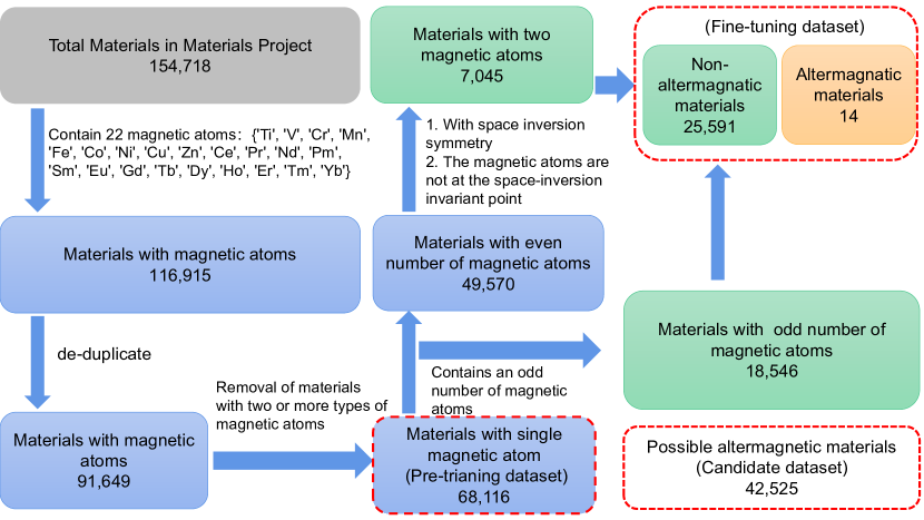
Extended Data Figure 1: The workflow for screening altermagnetic materials based on symmetry analysis. Through this screening process, we can build datasets for pre-training and fine-tuning, as well as a candidate set of possible altermagnetic materials.

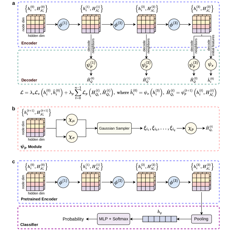
Extended Data Figure 2: The network architectures of the auto-encoder and the classifier. a, Details of the auto-encoder model. The encoder consists of three graph convolution layers denoted by $\phi^{(1)},\phi^{(3)},\phi^{(4)}$, whose input are node features $h_{i}^{(t)}$ and neighbors features $H_{\mathcal{N}_{i}}^{(t)}$, where $t=0,1,2$, respectively. The decoder is composed of a decoder module $\psi_{s}$ for reconstructing initial node features and three decoder modules $\psi_{p}^{(1)},\psi_{p}^{(2)},\psi_{p}^{(3)}$ for reconstructing neighborhood set of node features. We minimize the weighted sum of the reconstruction loss functions for both decoder modules. b, Details of the $\psi_{p}$ module in the decoder. The $\psi_{p}$ module includes three MLPs ($\chi_{\mu},\chi_{\sigma}$ and $\chi_{p}$) and a Gaussian sampler, while the $\psi_{s}$ module is composed of a single MLP. c, Details of the classifier model. The node features $h_{i}^{(0)}$ and the neighborhood set of node features $H_{\mathcal{N}_{i}}^{(0)}$ are fed into the pre-trained encoder. The output node features ${h}_{i}^{(3)}$ are then transformed to a latent vector ${h}_{g}$ by a pooling layer. Finally, another MLP and softmax module is designed to output the probability that quantifies whether the material is altermagnetic.

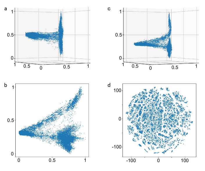
Extended Data Figure 3: Visualization of the learned crystal embeddings of the candidate materials, projected into 20 principal components by PCA. a, b, c Pair-wise visualization of three or two selected principal components of the learned crystal embeddings. d The t-distributed stochastic neighbor embedding (t-SNE) plot of the 20 principal components, revealing obvious clustering phenomena.

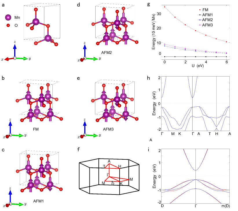
Extended Data Figure 4: The crystal and electronic structure of the altermagnet $MnO$. a, The crystal primitive cell of altermagnetic $MnO$. b, c, d, and e, The four significant magnetic structures $MnO$. The arrows represent magnetic moments of $Mn$. f, The Brillouin zone (BZ) with high-symmetry points and lines of altermagnetic $MnO$. g, The relative energy of four significant magnetic states with the variation of correlation interaction U. h and i, The electronic band structure of $MnO$ along high-symmetry directions and non-high-symmetry directions without spin-orbit coupling (SOC), respectively. The red and blue lines represent the spin-up and spin-down energy bands, respectively. The electronic structure is calculated under correlation interaction $\rm{U=4\leavevmode\nobreak\ eV}$.

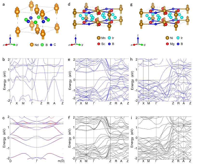
Extended Data Figure 5: The crystal and electronic structure of the altermagnet $NdB_{2}C_{2}$. a, The $NdB_{2}C_{2}$ crystal primitive cell with magnetic structure. b and c, The electronic band structure of altermagnetic $NdB_{2}C_{2}$. The electronic structure is calculated under correlation interaction $\rm{U=5\leavevmode\nobreak\ eV}$. d, The $Sc_{2}MnIr_{5}B_{2}$ crystal primitive cell with magnetic structure. e and f, The electronic band structure of altermagnetic $Sc_{2}MnIr_{5}B_{2}$ without and with SOC, respectively. The electronic structure is calculated under correlation interaction $\rm{U=4\leavevmode\nobreak\ eV}$. g, The $Mg_{2}NiIr_{5}B_{2}$ crystal primitive cell with magnetic structure. h and i, The electronic band structure of altermagnetic $Mg_{2}NiIr_{5}B_{2}$ without and with SOC, respectively. The electronic structure is calculated under correlation interaction $\rm{U=6.56\leavevmode\nobreak\ eV}$. The red and blue lines represent spin-up and spin-down energy bands, respectively.

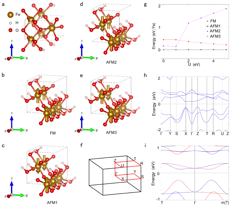
Extended Data Figure 6: The crystal and electronic structure of the altermagnet $FeHO_{2}$. a, The crystal primitive cell of the altermagnetic $FeHO_{2}$. b, c, d and e, Four significant magnetic structure of $FeHO_{2}$. The arrows represent magnetic moments of $Fe$. f, The Brillouin zone (BZ) with high-symmetry points and lines of altermagnetic $FeHO_{2}$. g, The relative energy of four significant magnetic states with the variation of correlation interaction U. h and i, The electronic band structure of $FeHO_{2}$ without SOC. The red and blue lines represent the spin-up and spin-down energy bands, respectively. The electronic structure is calculated under correlation interaction $\rm{U=4\leavevmode\nobreak\ eV}$.

This supplementary document provides a detailed description of the proposed pre-trained model, dataset statistics, hyperparameter value, and details of altermagnetic materials confirmed by electronic structure calculations.

A Addition information for pre-trained model

Model architecture

We have two models in total, which are the auto-encoder model and the classifier model. Extended Data Fig. 2 shows the overall architecture and details of models. We pre-process the crystals and construct a graph for each crystal according to its structure and atoms. In Extended Data Fig. 2, $\bm{\mu}_{v}$ stands for features from the crystal graph.

Learning curve of auto-encoder

We pre-train our auto-encoder model for only 10 epochs. To show the changing trend of pre-train loss, we choose the number of batch as the $x$-coordinate instead of epochs in Fig. S.1.

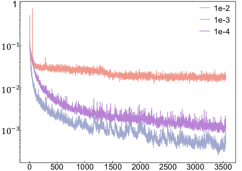
Figure S.1: Learning curve of the auto-encoder model with vary learning rate. The $x$-coordinate is the number of batches while the $y$-coordinate is the MSE loss.

Details for pre-process

The 3-dim crystal structure is straightforward and intuitive, but it is awkward to deal with in code. Thus, the crystal graph arises from the 3-dim crystal structure. The part of negligible information is not significant, such as the weak bonds. The nodes and edges represent the atoms and bonds, respectively. The nodes are connected with edges. We still retain the important information of atoms and bonds. The magnetic atoms are extracted with the corresponding weight function. We are concerned with the material information of altermagnetic, which is critical and indispensable.

The feature vector $h$ is used throughout in each step. In order to make it easier to understand, we are going to expand on it. The feature vector $h$ is analogous to the occupation number representation in quantum mechanics with the range from unoccupied 0 to occupied 1. The occupancy probability given by the subsequent iterations is still between 0 and 1 and it is the superposition of the wannier wave functions of the unoccupied state and occupied state. The element order information in the feature vector $h$ is read from the structure file, and the order is fixed. There is also a significant eigenvector $z$, which is effective in complementing the information about the interaction strength of the bonds. The initial eigenvector $u(i,j)_{k}$ has only two values of 0 and 1, without bond 0 and with bond 1. However, the strong and weak information will be manifested by the relative magnitude with the range from 0 and 1 in the subsequent iterations. The stronger bonds will be close to 1, and the weaker bonds will be close to 0. An example of pre-processing for $FeB$ to graph representation is shown in Fig. S.2.

Figure S.2: An example of pre-processing for crystal structure to crystal graph representation. The green nodes denote the $B$ atoms, and the brown nodes denote the $Fe$ atoms. The $Fe1$ node connects $B1$, $B2$, $B3$ and $B4$ nodes by 4 edges. It is pronounced that the $Fe2$ node connects the $B1$ and $B4$ nodes. The $Fe$ nodes are consistent with each other in the 4 corners with periodic boundary conditions. Thus, the $Fe2$ node connects $B1$, $B2$, $B3$ and $B4$ nodes as well as $Fe1$ node. Furthermore, the top $B2$ node connects the bottom $B1$ node, and the left $B3$ node connects the right $B4$ node.

Hyperparameter value

Table S.1: Hyperparameter value obtained by grid search.

Hyperparameter	Auto-encoder	Classifier	Description
Epochs	10	500	Training epoch
Learning rate	1.0e-3	1.0e-3	Learning rate for optimizing neural network
Batch size	64	512	Number of input token per batch
Hidden dimension	512	512	Size of dimensions in the graph convolution layer
Sample size	10	-	Number of samples during the reconstruction
Radius	20	20	Neighbor distance of crystal atoms
Drop rate	-	0.25	Dropout rate for Classifier

In the pre-processing procedure, the crystal structure files (.cif) are transformed to the crystal graph data which can be fed into the model directly. Nodes of the graph are represented from atoms naturally and the atoms will be regraded as the neighbors of another atom if they are in the unit cell, out to a distance of radius. In the pre-training procedure, using the pre-training dataset consisting of the 25,591 non-altermagnetic materials and the 42,525 candidate materials, we pre-train our auto-encoder model for 10 epochs with a batch size of 64 on 2 NVIDIA A100 GPUs, which takes about 2 days. Once pre-training is over, we load the weights of the encoder module into the classifier model and begin training for 500 epochs with a batch size of 512 and a drop rate of 0.25. The learning rate of both models is $1.0e-3$ and hidden dimension of the encoder module is 512.

B Addition altermagnetic materials confirmed by electronic structure calculations

For the remaining 19 materials ($NaFeO_{2}(31)$, $MnO_{2}(62)$, $MnO_{2}(87)$, $CaLaCr_{2}O_{6}$, $Ca_{3}Cr_{2}O_{7}$, $CaLaFeAgO_{6}$, $ZrCrO_{3}$, $ZrMnO_{3}$, $VF_{3}$, $CrF_{3}$, $FeF_{3}$, $CoF_{3}$, $NiF_{3}$, $CaMnN_{2}$, $Ir_{5}B_{2}Mg_{2}Fe$, $Ir_{5}B_{2}Mg_{2}Mn$, $Ir_{5}B_{2}Mg_{2}Ni$, $Ir_{5}B_{2}Sc_{2}V$, $Ir_{5}B_{2}Sc_{2}Mn$), we determine their magnetic ground states by calculating the energies of their different magnetic structures under different correlated interactions U. Then, symmetry analysis is used to determine that these magnetic ground states are altermagnetic states. Furthermore, symmetry analysis is also used to determine whether these altermagnetic materials are $d$-wave, $g$-wave or $i$-wave. Finally, the electronic band structures are used to demonstrate our symmetry analysis. All calculated results are shown in Fig. S.3 - S.13.

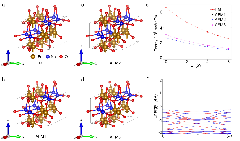
Figure S.3: Altermagnetic $NaFeO_{2}(33)$ is confirmed by electronic structure calculations. a, b, c, and d are crystal structures of the $NaFeO_{2}(33)$ with FM, AFM1, AFM2 and AFM3 magnetic structures, respectively. The arrows represent magnetic moments of $Fe$. e represents the relative energy of four magnetic states with the variation of correlation interaction U. f represents the electronic band structure of $NaFeO_{2}(33)$ along non-high-symmetry directions without SOC. The red and blue lines represent the spin-up and spin-down energy bands, respectively. The electronic structure is calculated under correlation interaction $\rm{U=4\leavevmode\nobreak\ eV}$.

Figure S.4: Altermagnetic $MnO_{2}(62)$ is confirmed by electronic structure calculations. a, b, c, and d are crystal structures of the $MnO_{2}(62)$ with FM, AFM1, AFM2 and AFM3 magnetic structures, respectively. The arrows represent magnetic moments of $Mn$. e represents the relative energy of four magnetic states with the variation of correlation interaction U. f represents the electronic band structure along non-high-symmetry directions without SOC. The red and blue lines represent the spin-up and spin-down energy bands, respectively. The electronic structure is calculated under correlation interaction $\rm{U=4\leavevmode\nobreak\ eV}$.

Figure S.5: Altermagnetic $MnO_{2}(87)$ is confirmed by electronic structure calculations. a, b, c, and d are crystal structures of the $MnO_{2}(87)$ with FM, AFM1, AFM2 and AFM3 magnetic structures, respectively. The arrows represent magnetic moments of $Mn$. e represents the relative energy of four magnetic states with the variation of correlation interaction U. f represents the electronic band structure along non-high-symmetry directions without SOC. The red and blue lines represent the spin-up and spin-down energy bands, respectively. The electronic structure is calculated under correlation interaction $\rm{U=4\leavevmode\nobreak\ eV}$.

Figure S.6: Altermagnetic $CaLaCr_{2}O_{6}$ is confirmed by electronic structure calculations. a, b, c, and d are crystal structures of the $CaLaCr_{2}O_{6}$ with FM, AFM1, AFM2 and AFM3 magnetic structures, respectively. The arrows represent magnetic moments of $Cr$. e represents the relative energy of four magnetic states with the variation of correlation interaction U. f represents the electronic band structure along non-high-symmetry directions without SOC. The red and blue lines represent the spin-up and spin-down energy bands, respectively. The electronic structure is calculated under correlation interaction $\rm{U=4\leavevmode\nobreak\ eV}$.

Figure S.7: Altermagnetic $Ca_{3}Cr_{2}O_{7}$ is confirmed by electronic structure calculations. a, b, c, and d are crystal structures of the $Ca_{3}Cr_{2}O_{7}$ with FM, AFM1, AFM2 and AFM3 magnetic structures, respectively. The arrows represent magnetic moments of $Cr$. e represents the relative energy of four magnetic states with the variation of correlation interaction U. f represents the electronic band structure along non-high-symmetry directions without SOC. The red and blue lines represent the spin-up and spin-down energy bands, respectively. The electronic structure is calculated under correlation interaction $\rm{U=4\leavevmode\nobreak\ eV}$.

Figure S.8: The crystal and electronic structure of the altermagnetic $CaLaFeAgO_{6}$. a is the crystal primitive cell of altermagnetic $CaLaFeAgO_{6}$. b, c, d, and e are crystal structures of the $CaLaFeAgO_{6}$ with FM, AFM1, AFM2 and AFM3 magnetic structures, respectively. The arrows represent magnetic moments of $Fe$. f The Brillouin zone (BZ) with high-symmetry points and lines of altermagnetic $CaLaFeAgO_{6}$. g represents the relative energy of four magnetic states with the variation of correlation interaction U. h and i represent the electronic band structure along high-symmetry directions and non-high-symmetry directions without SOC, respectively. The red and blue lines represent the spin-up and spin-down energy bands, respectively. The electronic structure is calculated under correlation interaction $\rm{U=4\leavevmode\nobreak\ eV}$.

Figure S.9: Altermagnetic $ZrCrO_{3}$ is confirmed by electronic structure calculations. a, b, c, and d are crystal structures of the $ZrCrO_{3}$ with FM, AFM1, AFM2 and AFM3 magnetic structures, respectively. The arrows represent magnetic moments of $Cr$. e represents the relative energy of four magnetic states with the variation of correlation interaction U. f represents the electronic band structure along non-high-symmetry directions without SOC. The red and blue lines represent the spin-up and spin-down energy bands, respectively. The electronic structure is calculated under correlation interaction $\rm{U=4\leavevmode\nobreak\ eV}$.

Figure S.10: Altermagnetic $ZrMnO_{3}$ is confirmed by electronic structure calculations. a, b, c, and d are crystal structures of the $ZrMnO_{3}$ with FM, AFM1, AFM2 and AFM3 magnetic structures, respectively. The arrows represent magnetic moments of $Mn$. e represents the relative energy of four magnetic states with the variation of correlation interaction U. f represents the electronic band structure along non-high-symmetry directions without SOC. The red and blue lines represent the spin-up and spin-down energy bands, respectively. The electronic structure is calculated under correlation interaction $\rm{U=4\leavevmode\nobreak\ eV}$.

Figure S.11: The crystal and electronic structure of the altermagnetic $CaMnN_{2}$. a is the crystal primitive cell of altermagnetic $CaMnN_{2}$. b, c, d, and e are crystal structures of the $CaMnN_{2}$ with FM, AFM1, AFM2 and AFM3 magnetic structures, respectively. The arrows represent magnetic moments of $Mn$. f The Brillouin zone (BZ) with high-symmetry points and lines of altermagnetic $CaMnN_{2}$. g represents the relative energy of four magnetic states with the variation of correlation interaction U. h and i represent the electronic band structure along high-symmetry directions and non-high-symmetry directions without SOC, respectively. The red and blue lines represent the spin-up and spin-down energy bands, respectively. The electronic structure is calculated under correlation interaction $\rm{U=4\leavevmode\nobreak\ eV}$.

Figure S.12: Altermagnetic materials are confirmed by electronic structure calculations. a is the crystal primitive cell. b,c,d,e are crystal structures of the $Ir_{5}B_{2}Y_{2}X\leavevmode\nobreak\ (Y=Mg,Sc,X=Fe,Mn,Ni,V)$ with FM, AFM1, AFM2 and AFM3 magnetic structures, respectively. f,g,h,i,j Relative energy of four significant magnetic states with the variation of correlation interaction U of $Ir_{5}B_{2}Mg_{2}Fe$, $Ir_{5}B_{2}Mg_{2}Mn$, $Ir_{5}B_{2}Mg_{2}Ni$, $Ir_{5}B_{2}Sc_{2}V$ and $Ir_{5}B_{2}Sc_{2}Mn$. The k,l,m,n,o are the electronic band structure of altermagnetic $Ir_{5}B_{2}Y_{2}X$ along non-high-symmetry directions without SOC. The red and blue lines represent spin-up and spin-down energy bands, respectively.

Figure S.13: Altermagnetic materials are confirmed by electronic structure calculations. The crystal primitive cell and Brillouin Zone (BZ) are illustrated by a. b,c,d,e are crystal structures of $XF_{3}\leavevmode\nobreak\ (X=V,Cr,Fe,Co,Ni)$ with FM, AFM1, AFM2 and AFM3 magnetic structures, respectively. f,g,h,i,j Relative energy of four significant magnetic states with the variation of correlation interaction U of $VF_{3}$, $CrF_{3}$, $FeF_{3}$, $CoF_{3}$ and $NiF_{3}$. The k,l,m,n,o are the electronic band structure of altermagnetic $XF_{3}$ along non-high-symmetry directions without SOC. The red and blue lines represent spin-up and spin-down energy bands, respectively. The electronic structure is calculated under correlation interaction $\rm{U=4\leavevmode\nobreak\ eV}$.

Table S.2: The band gap of the 14 altermagentic insulator materials under the LDA+U framework.

Number	Materials	Gap/eV
1	$FeHO_{2}$	0.37
2	$NaFeO_{2}$	3.18
3	$NaFeO_{2}$	3.11
4	$MnO_{2}$	1.60
5	$MnO_{2}$	1.73
6	$Ca_{3}Cr_{2}O_{7}$	1.34
7	$ZrCrO_{3}$	1.86
8	$ZrMnO_{3}$	3.47
9	$VF_{3}$	2.87
10	$CrF_{3}$	4.13
11	$FeF_{3}$	3.63
12	$CoF_{3}$	2.19
13	$MnO$	0.65
14	$CaMnN_{2}$	0.95

References

- [1] Libor Šmejkal, Jairo Sinova, and Tomas Jungwirth. Beyond conventional ferromagnetism and antiferromagnetism: A phase with nonrelativistic spin and crystal rotation symmetry. Phys. Rev. X, 12:031042, Sep 2022.
- [2] Libor Šmejkal, Jairo Sinova, and Tomas Jungwirth. Emerging research landscape of altermagnetism. Phys. Rev. X, 12:040501, Dec 2022.
- [3] Libor Šmejkal, Anna Birk Hellenes, Rafael González-Hernández, Jairo Sinova, and Tomas Jungwirth. Giant and tunneling magnetoresistance in unconventional collinear antiferromagnets with nonrelativistic spin-momentum coupling. Phys. Rev. X, 12:011028, Feb 2022.
- [4] Rafael González-Hernández, Libor Šmejkal, Karel Výborný, Yuta Yahagi, Jairo Sinova, Tomá š Jungwirth, and Jakub Železný. Efficient electrical spin splitter based on nonrelativistic collinear antiferromagnetism. Phys. Rev. Lett., 126:127701, Mar 2021.
- [5] H. Bai, L. Han, X. Y. Feng, Y. J. Zhou, R. X. Su, Q. Wang, L. Y. Liao, W. X. Zhu, X. Z. Chen, F. Pan, X. L. Fan, and C. Song. Observation of spin splitting torque in a collinear antiferromagnet . Phys. Rev. Lett., 128:197202, May 2022.
- [6] Arnab Bose, Nathaniel J Schreiber, Rakshit Jain, Ding-Fu Shao, Hari P Nair, Jiaxin Sun, Xiyue S Zhang, David A Muller, Evgeny Y Tsymbal, Darrell G Schlom, et al. Tilted spin current generated by the collinear antiferromagnet ruthenium dioxide. Nat. Electron., 2022.
- [7] Peng-Jie Guo, Zheng-Xin Liu, and Zhong-Yi Lu. Quantum anomalous hall effect in collinear antiferromagnetism. npj Comput. Mater., 9(1):70, May 2023.
- [8] Libor Šmejkal, Rafael Gonzalez-Hernandez, T. Jungwirth, and J. Sinova. Crystal time-reversal symmetry breaking and spontaneous hall effect in collinear antiferromagnets. Sci. Adv., 6:eaaz8809, 2020.
- [9] Libor Šmejkal, Allan H. MacDonald, Jairo Sinova, Satoru Nakatsuji, and Tomas Jungwirth. Anomalous hall antiferromagnets. Nat. Rev. Mater., 7:482, Jun 2022.
- [10] Xiaodong Zhou, Wanxiang Feng, Xiuxian Yang, Guang-Yu Guo, and Yugui Yao. Crystal chirality magneto-optical effects in collinear antiferromagnets. Phys. Rev. B, 104:024401, Jul 2021.
- [11] Zexin Feng, Xiaorong Zhou, Libor Šmejkal, Lei Wu, Huixin Guo, Rafael González-Hernández, Xiaoning Wang, Han Yan, Peixin Qin, Xin Zhang, Haojiang Wu, Hongyu Chen, Ziang Meng, Li Liu, Zhengcai Xia, Jairo Sinova, Tomáš Jungwirth, and Zhiqi Liu. An anomalous hall effect in altermagnetic ruthenium dioxide. Nat. Electron., 2022.
- [12] R. D. Gonzalez Betancourt, J. Zubáč, R. Gonzalez-Hernandez, K. Geishendorf, Z. Šobáň, G. Springholz, K. Olejník, L. Šmejkal, J. Sinova, T. Jungwirth, S. T. B. Goennenwein, A. Thomas, H. Reichlová, J. Železný, and D. Kriegner. Spontaneous anomalous hall effect arising from an unconventional compensated magnetic phase in a semiconductor. Phys. Rev. Lett., 130:036702, Jan 2023.
- [13] Peng-Jie Guo, Yi-Wen Wei, Kai Liu, Zheng-Xin Liu, and Zhong-Yi Lu. Eightfold degenerate fermions in two dimensions. Phys. Rev. Lett., 127:176401, Oct 2021.
- [14] Pengfei Liu, Jiayu Li, Jingzhi Han, Xiangang Wan, and Qihang Liu. Spin-group symmetry in magnetic materials with negligible spin-orbit coupling. Phys. Rev. X, 12:021016, Apr 2022.
- [15] Jian Yang, Zheng-Xin Liu, and Chen Fang. Symmetry invariants in magnetically ordered systems having weak spin-orbit coupling. ArXiv:, 2105:12738, May 2021.
- [16] R Jaeschke-Ubiergo, VK Bharadwaj, L Šmejkal, and Jairo Sinova. Supercell altermagnets. ArXiv:, 2308:16662, Aug 2023.
- [17] Hanchen Wang, Tianfan Fu, Yuanqi Du, Wenhao Gao, Kexin Huang, Ziming Liu, Payal Chandak, Shengchao Liu, Peter Van Katwyk, Andreea Deac, et al. Scientific discovery in the age of artificial intelligence. Nature, 620(7972):47–60, 2023.
- [18] David C Blakemore, Luis Castro, Ian Churcher, David C Rees, Andrew W Thomas, David M Wilson, and Anthony Wood. Organic synthesis provides opportunities to transform drug discovery. Nature Chem., 10(4):383–394, 2018.
- [19] Marwin HS Segler, Mike Preuss, and Mark P Waller. Planning chemical syntheses with deep neural networks and symbolic AI. Nature, 555(7698):604–610, 2018.
- [20] Jonathan W Lehmann, Daniel J Blair, and Martin D Burke. Towards the generalized iterative synthesis of small molecules. Nat. Rev. Chem., 2(2):0115, 2018.
- [21] Rohit Batra, Troy D Loeffler, Henry Chan, Srilok Srinivasan, Honggang Cui, Ivan V Korendovych, Vikas Nanda, Liam C Palmer, Lee A Solomon, H Christopher Fry, et al. Machine learning overcomes human bias in the discovery of self-assembling peptides. Nature Chem., 14(12):1427–1435, 2022.
- [22] Tian Xie and Jeffrey C Grossman. Crystal graph convolutional neural networks for an accurate and interpretable prediction of material properties. Phys. Rev. Lett., 120(14):145301, 2018.
- [23] Gus LW Hart, Tim Mueller, Cormac Toher, and Stefano Curtarolo. Machine learning for alloys. Nat. Rev. Mater., 6(8):730–755, 2021.
- [24] Weihua Hu, Bowen Liu, Joseph Gomes, Marinka Zitnik, Percy Liang, Vijay S. Pande, and Jure Leskovec. Strategies for pre-training graph neural networks. In ICLR, 2020.
- [25] Ludger Rüschendorf. The wasserstein distance and approximation theorems. Probab. Theory Relat. Fields, 70(1):117–129, 1985.
- [26] Olexandr Isayev, Denis Fourches, Eugene N. Muratov, Corey Oses, Kevin Rasch, Alexander Tropsha, and Stefano Curtarolo. Materials cartography: Representing and mining materials space using structural and electronic fingerprints. Chem. Mater., 27(3):735–743, 2015.
- [27] Anubhav Jain, Joseph Montoya, Shyam Dwaraknath, Nils E. R. Zimmermann, John Dagdelen, Matthew Horton, Patrick Huck, Donny Winston, Shreyas Cholia, Shyue Ping Ong, and Kristin Persson. The materials project: Accelerating materials design through theory-driven data and tools. In Handbook of Materials Modeling: Methods: Theory and Modeling, pages 1751–1784. Springer, 2020.
- [28] Jacob Devlin, Ming-Wei Chang, Kenton Lee, and Kristina Toutanova. BERT: pre-training of deep bidirectional transformers for language understanding. In NAACL, pages 4171–4186, 2019.
- [29] René Ranftl, Alexey Bochkovskiy, and Vladlen Koltun. Vision transformers for dense prediction. In ICCV, pages 12179–12188, 2021.
- [30] Patrick Cramer. Alphafold2 and the future of structural biology. Nat. Struct. Mol. Biol., 28(9):704–705, 2021.
- [31] Mingyue Tang, Pan Li, and Carl Yang. Graph auto-encoder via neighborhood wasserstein reconstruction. In ICLR, 2022.
- [32] Kenji Ohoyama, Takahiro Onimaru, Hideya Onodera, Hiroki Yamauchi, and Yasuo Yamaguchi. Antiferromagnetic structure with the uniaxial anisotropy in the tetragonal type compound, . J. Phys. Soc. Japan, 69:2623, Aug 2000.
- [33] Op Baburova, Iub Kuzma, and Ti Tsolkovskii. The systems niobium-iron-boron and niobium- cobalt-boron (phase equilibria in ternary systems -- and --, determining structural types and lattice constants by using X ray and microstructural analysis). Inorg. Mater., 4:950–953, 1968.
- [34] Kuz’ma, Yu.B., A.S. Sobolev, Fedorov, and T.F. Phase equilibria in the ternary systems tantalum-iron-boron and tantalum-nickel-boron. Powder Metall. Met. Ceram., 5:410–414, 1971.
- [35] Jung W. and Schiffer J. Quaternäre magnesium-iridiumboride mit - eine besetzungsvariante des -typs. Z. Anorg. Allg. Chem., 581:135–140, 1990.
- [36] E A Nagelschmitz and W Jung. Scandium iridium boride and the quaternary derivatives with : Preparation, crystal structure, and physical properties. Chem. Mater., 10(10), 10 1998.
- [37] Daniel P., Bulou A., Leblanc M., Rousseau M., and Nouet J. Structural and vibrational study of v f3. Mater. Res. Bull., 25:413–420, 1990.
- [38] Bolotina N.B., Molchanov V.N., Dyuzheva T.I., Lityagina L.M., and Bendeliani N.A. Single-crystal structures of high-pressure phases FeOOH, FeOOD, and GaOOH. Kristallografiya, 53:1017–1022, 2008.
- [39] Grey I.E., Hoskins B.F., and I.C. Madsen. A structural study of the incorporation of silica into sodium ferrites, . J. Solid State Chem., 85:202–219, 1990.
- [40] Grey I.E., Hill R.J., and Hewat A.W. A neutron powder diffraction study of the beta to gamma phase transformation in . Z. Kristallogr. Cryst. Mater., 193:51–69, 1990.
- [41] Curetti Nadia, Bernasconi Davide, Benna Piera, Fiore Gianluca, and Pavese Alessandro. High-temperature ramsdellite-pyrolusite transformation kinetics. Phys. Chem. Miner., 48, 2021.
- [42] Kondrashev Yu.D. and Zaslavskii A.I. The structure of the modifications of manganese oxide. Izv. Acad. Nauk SSSR, Ser. Fiz., 15:179–186, 1951.
- [43] Khan M. Alam, Dongwook Han, Lee Gihyeok, Kim Yong-Il, and Kang Yong-Mook. phase-integrated cathode materials for sodium-ion rechargeable batteries. J. Alloys Compd., 771:987–993, 2019.
- [44] Xiao-Yao Hou, Huan-Cheng Yang, Zheng-Xin Liu, Peng-Jie Guo, and Zhong-Yi Lu. Large intrinsic anomalous hall effect in both and with collinear antiferromagnetism. Phys. Rev. B, 107:L161109, Apr 2023.
- [45] S. L. Dudarev, G. A. Botton, S. Y. Savrasov, C. J. Humphreys, and A. P. Sutton. Electron-energy-loss spectra and the structural stability of nickel oxide: An study. Phys. Rev. B, 57:1505–1509, Jan 1998.
- [46] Zeyu Jiang, Wenkai Lou, Yu Liu, Yuanchang Li, Haifeng Song, Kai Chang, Wenhui Duan, and Shengbai Zhang. Spin-triplet excitonic insulator: The case of semihydrogenated graphene. Phys. Rev. Lett., 124:166401, Apr 2020.
- [47] Alec Radford, Jeffrey Wu, Rewon Child, David Luan, Dario Amodei, Ilya Sutskever, et al. Language models are unsupervised multitask learners. OpenAI blog, 1(8):9, 2019.
- [48] G. Kresse and J. Furthmüller. Efficient iterative schemes for ab initio total-energy calculations using a plane-wave basis set. Phys. Rev. B, 54:11169–11186, Oct 1996.
- [49] John P. Perdew, Kieron Burke, and Matthias Ernzerhof. Generalized gradient approximation made simple. Phys. Rev. Lett., 77:3865–3868, Oct 1996.
- [50] P. E. Blöchl. Projector augmented-wave method. Phys. Rev. B, 50:17953–17979, Dec 1994.