Validation of tight-binding model in system of two semiconductor single-electron lines coupled electrostatically by Schrödinger formalism
*
Krzysztof Pomorski1,2
1: Institute of Physics, Lodz University of Technology, Lodz, Poland
2: Quantum Hardware Systems, Lodz, Poland
Abstract
Validation of tight-binding model is given basing on two single-electron lines coupled perturbatively electrostatically in Schrödinger formalism.
Scheme for conversion of quantum information from eigenenergy qubits to position based qubits is given.
The procedure for determination of system ground is presented. Additional extension schemes of two coupled single-electron lines in case of Rabi oscillations occurring in each position based qubits are given.
Index Terms:
single-electron line, position-based qubits, quantum swap gate, Rabi oscillations
I Introduction to position-based qubits
Currently there is worldwide race in development of quantum technologies leading to
new quantum computation platforms, quantum communication and quantum metrology systems [1 ] , [2 ] . Due to integration possibility
the dominant technology platforms are mesoscopic superconducting structures and nano-size semiconductor electronic elements as coupled semiconductor quantum dots or
miniaturized cryogenic CMOS circuits. Starting from eigenergy qubit as given by IBM Q-Experience or many other technologies (| γ E 1 ( t ) | 2 + | γ E 2 ( t ) | 2 = 1 superscript subscript 𝛾 𝐸 1 𝑡 2 superscript subscript 𝛾 𝐸 2 𝑡 2 1 |\gamma_{E1}(t)|^{2}+|\gamma_{E2}(t)|^{2}=1
H ^ ( t ) E | ψ ( t ) ⟩ E = ( E 1 → 1 ( t ) E 2 → 1 ( t ) E 1 → 2 ( t ) E 2 → 2 ( t ) ) E ( γ E 1 ( t ) γ E 2 ( t ) ) E = ^ 𝐻 subscript 𝑡 𝐸 subscript ket 𝜓 𝑡 𝐸 subscript matrix subscript 𝐸 → 1 1 𝑡 subscript 𝐸 → 2 1 𝑡 subscript 𝐸 → 1 2 𝑡 subscript 𝐸 → 2 2 𝑡 𝐸 subscript matrix subscript 𝛾 𝐸 1 𝑡 subscript 𝛾 𝐸 2 𝑡 𝐸 absent \displaystyle\hat{H}(t)_{E}\ket{\psi(t)}_{E}=\begin{pmatrix}E_{1\rightarrow 1}(t)&E_{2\rightarrow 1}(t)\\
E_{1\rightarrow 2}(t)&E_{2\rightarrow 2}(t)\end{pmatrix}_{E}\begin{pmatrix}\gamma_{E1}(t)\\
\gamma_{E2}(t)\end{pmatrix}_{E}=
= i ℏ d d t ( γ E 1 ( t ) γ E 2 ( t ) ) E = i ℏ d d t ( | ψ ( t ) ⟩ ) E = absent 𝑖 Planck-constant-over-2-pi 𝑑 𝑑 𝑡 subscript matrix subscript 𝛾 𝐸 1 𝑡 subscript 𝛾 𝐸 2 𝑡 𝐸 𝑖 Planck-constant-over-2-pi 𝑑 𝑑 𝑡 subscript ket 𝜓 𝑡 𝐸 absent \displaystyle=i\hbar\frac{d}{dt}\begin{pmatrix}\gamma_{E1}(t)\\
\gamma_{E2}(t)\end{pmatrix}_{E}=i\hbar\frac{d}{dt}(\ket{\psi(t)})_{E}=
= i ℏ d d t ( γ E 1 ( t ) | E 1 ( t ) ⟩ + γ E 2 ( t ) | E 2 ( t ) ⟩ ) = absent 𝑖 Planck-constant-over-2-pi 𝑑 𝑑 𝑡 subscript 𝛾 𝐸 1 𝑡 ket subscript 𝐸 1 𝑡 subscript 𝛾 𝐸 2 𝑡 ket subscript 𝐸 2 𝑡 absent \displaystyle=i\hbar\frac{d}{dt}(\gamma_{E1}(t)\ket{E_{1}(t)}+\gamma_{E2}(t)\ket{E_{2}(t)})=
= ( E 1 → 1 ( t ) E 2 → 1 ( t ) E 1 → 2 ( t ) E 2 → 2 ( t ) ) E ( + cos ( Θ ) − sin ( Θ ) + sin ( Θ ) + cos ( Θ ) ) × \displaystyle=\begin{pmatrix}E_{1\rightarrow 1}(t)&E_{2\rightarrow 1}(t)\\
E_{1\rightarrow 2}(t)&E_{2\rightarrow 2}(t)\end{pmatrix}_{E}\begin{pmatrix}+\cos(\Theta)&-\sin(\Theta)\\
+\sin(\Theta)&+\cos(\Theta)\end{pmatrix}\times
× ( + cos ( Θ ) + sin ( Θ ) − sin ( Θ ) + cos ( Θ ) ) ( γ E 1 ( t ) γ E 2 ( t ) ) E = \displaystyle\times\begin{pmatrix}+\cos(\Theta)&+\sin(\Theta)\\
-\sin(\Theta)&+\cos(\Theta)\end{pmatrix}\begin{pmatrix}\gamma_{E1}(t)\\
\gamma_{E2}(t)\end{pmatrix}_{E}=
i ℏ d d t [ ( + cos ( Θ ) − sin ( Θ ) + sin ( Θ ) + cos ( Θ ) ) × \displaystyle i\hbar\frac{d}{dt}\Bigg{[}\begin{pmatrix}+\cos(\Theta)&-\sin(\Theta)\\
+\sin(\Theta)&+\cos(\Theta)\end{pmatrix}\times
× ( + cos ( Θ ) + sin ( Θ ) − sin ( Θ ) + cos ( Θ ) ) ( γ E 1 ( t ) γ E 2 ( t ) ) E ] \displaystyle\times\begin{pmatrix}+\cos(\Theta)&+\sin(\Theta)\\
-\sin(\Theta)&+\cos(\Theta)\end{pmatrix}\begin{pmatrix}\gamma_{E1}(t)\\
\gamma_{E2}(t)\end{pmatrix}_{E}\Bigg{]} (1)
where we have E s → k ( t ) = ⟨ E k ( t ) | H ^ ( t ) | E s ( t ) ⟩ subscript 𝐸 → 𝑠 𝑘 𝑡 bra subscript 𝐸 𝑘 𝑡 ^ 𝐻 𝑡 ket subscript 𝐸 𝑠 𝑡 E_{s\rightarrow k}(t)=\bra{E_{k}(t)}\hat{H}(t)\ket{E_{s}(t)} H ^ ( t ) = E 1 → 1 ( t ) | E 1 ( t ) ⟩ ⟨ E 1 ( t ) | + E 2 → 2 ( t ) | E 2 ( t ) ⟩ ⟨ E 2 ( t ) | + E 1 → 2 ( t ) | E 2 ( t ) ⟩ ⟨ E 1 ( t ) | + E 2 → 1 ( t ) | E 1 ( t ) ⟩ ⟨ E 2 ( t ) | ^ 𝐻 𝑡 subscript 𝐸 → 1 1 𝑡 ket subscript 𝐸 1 𝑡 bra subscript 𝐸 1 𝑡 subscript 𝐸 → 2 2 𝑡 ket subscript 𝐸 2 𝑡 bra subscript 𝐸 2 𝑡 subscript 𝐸 → 1 2 𝑡 ket subscript 𝐸 2 𝑡 bra subscript 𝐸 1 𝑡 subscript 𝐸 → 2 1 𝑡 ket subscript 𝐸 1 𝑡 bra subscript 𝐸 2 𝑡 \hat{H}(t)=E_{1\rightarrow 1}(t)\ket{E_{1}(t)}\bra{E_{1}(t)}+E_{2\rightarrow 2}(t)\ket{E_{2}(t)}\bra{E_{2}(t)}+E_{1\rightarrow 2}(t)\ket{E_{2}(t)}\bra{E_{1}(t)}+E_{2\rightarrow 1}(t)\ket{E_{1}(t)}\bra{E_{2}(t)} | γ E 1 ( t ) | 2 superscript subscript 𝛾 𝐸 1 𝑡 2 |\gamma_{E1}(t)|^{2} | γ E 2 ( t ) | 2 superscript subscript 𝛾 𝐸 2 𝑡 2 |\gamma_{E2}(t)|^{2} E 1 subscript 𝐸 1 E_{1} E 2 subscript 𝐸 2 E_{2} Θ ( t ) Θ 𝑡 \Theta(t) ϕ ( t ) italic-ϕ 𝑡 \phi(t) | ψ ⟩ E = γ E 1 ( t ) | E 1 ( t ) ⟩ + γ E 2 ( t ) | E 2 ( t ) ⟩ = = e i ϕ 0 ( t ) ( c o s ( Θ ( t ) ) | E 1 ( t ) ⟩ + e i ϕ ( t ) s i n ( Θ ( t ) ) | E 2 ( t ) ⟩ ) \ket{\psi}_{E}=\gamma_{E1}(t)\ket{E_{1}(t)}+\gamma_{E2}(t)\ket{E_{2}(t)}=\\
=e^{i\phi_{0}(t)}(cos(\Theta(t))\ket{E_{1}(t)}+e^{i\phi(t)}sin(\Theta(t))\ket{E_{2}(t)}) 1 | α q ( t ) | 2 + | β q ( t ) | 2 = 1 superscript subscript 𝛼 𝑞 𝑡 2 superscript subscript 𝛽 𝑞 𝑡 2 1 |\alpha_{q}(t)|^{2}+|\beta_{q}(t)|^{2}=1
H ^ ( t ) W | ψ ( t ) ⟩ W = ( E p 1 ( t ) t s 12 ( t ) t s 12 ∗ ( t ) E p 2 ( t ) ) W ( α q ( t ) β q ( t ) ) W = ^ 𝐻 subscript 𝑡 𝑊 subscript ket 𝜓 𝑡 𝑊 subscript matrix subscript 𝐸 𝑝 1 𝑡 subscript 𝑡 𝑠 12 𝑡 superscript subscript 𝑡 𝑠 12 𝑡 subscript 𝐸 𝑝 2 𝑡 𝑊 subscript matrix subscript 𝛼 𝑞 𝑡 subscript 𝛽 𝑞 𝑡 𝑊 absent \displaystyle\hat{H}(t)_{W}\ket{\psi(t)}_{W}=\begin{pmatrix}E_{p1}(t)&t_{s12}(t)\\
t_{s12}^{*}(t)&E_{p2}(t)\end{pmatrix}_{W}\begin{pmatrix}\alpha_{q}(t)\\
\beta_{q}(t)\end{pmatrix}_{W}=
i ℏ d d t ( α q ( t ) | w L ( t ) ⟩ + β q ( t ) | w R ( t ) ⟩ ) W = i ℏ d d t | ψ ( t ) ⟩ W , 𝑖 Planck-constant-over-2-pi 𝑑 𝑑 𝑡 subscript subscript 𝛼 𝑞 𝑡 ket subscript 𝑤 𝐿 𝑡 subscript 𝛽 𝑞 𝑡 ket subscript 𝑤 𝑅 𝑡 𝑊 𝑖 Planck-constant-over-2-pi 𝑑 𝑑 𝑡 subscript ket 𝜓 𝑡 𝑊 \displaystyle i\hbar\frac{d}{dt}(\alpha_{q}(t)\ket{w_{L}(t)}+\beta_{q}(t)\ket{w_{R}(t)})_{W}=i\hbar\frac{d}{dt}\ket{\psi(t)}_{W}, (2)
where | w L ( t ) ⟩ ket subscript 𝑤 𝐿 𝑡 \ket{w_{L}(t)} | w R ( t ) ⟩ ket subscript 𝑤 𝑅 𝑡 \ket{w_{R}(t)} ⟨ w L | | w R ⟩ = 0 bra subscript 𝑤 𝐿 ket subscript 𝑤 𝑅 0 \bra{w_{L}}\ket{w_{R}}=0 ⟨ w L | | w L ⟩ = 1 = ⟨ w R | | w R ⟩ bra subscript 𝑤 𝐿 ket subscript 𝑤 𝐿 1 bra subscript 𝑤 𝑅 ket subscript 𝑤 𝑅 \bra{w_{L}}\ket{w_{L}}=1=\bra{w_{R}}\ket{w_{R}} | α q ( t ) | 2 superscript subscript 𝛼 𝑞 𝑡 2 |\alpha_{q}(t)|^{2} | β q ( t ) | 2 superscript subscript 𝛽 𝑞 𝑡 2 |\beta_{q}(t)|^{2} | ψ ( t ) ⟩ W subscript ket 𝜓 𝑡 𝑊 \ket{\psi(t)}_{W} | ψ ( t ) ⟩ E subscript ket 𝜓 𝑡 𝐸 \ket{\psi(t)}_{E}
Following [4 ] , [5 ] it will be useful to introduce parameter
r = ∫ − ∞ 0 𝑑 x ( ψ E 1 ( x ) ψ E 2 † ( x ) + ψ E 1 ( x ) † ψ E 2 ( x ) ) ∫ − ∞ 0 𝑑 x ( | ψ E 1 ( x ) | 2 − | ψ E 2 ( x ) | 2 ) . 𝑟 superscript subscript 0 differential-d 𝑥 subscript 𝜓 𝐸 1 𝑥 superscript subscript 𝜓 𝐸 2 † 𝑥 subscript 𝜓 𝐸 1 superscript 𝑥 † subscript 𝜓 𝐸 2 𝑥 superscript subscript 0 differential-d 𝑥 superscript subscript 𝜓 𝐸 1 𝑥 2 superscript subscript 𝜓 𝐸 2 𝑥 2 \displaystyle r=\frac{\int_{-\infty}^{0}dx(\psi_{E1}(x)\psi_{E2}^{{\dagger}}(x)+\psi_{E1}(x)^{{\dagger}}\psi_{E2}(x))}{\int_{-\infty}^{0}dx(|\psi_{E1}(x)|^{2}-|\psi_{E2}(x)|^{2})}. (3)
The precondition for occurrence of position-based qubit is occupancy at least two energetic levels, so neither | γ E 1 | 2 superscript subscript 𝛾 𝐸 1 2 |\gamma_{E1}|^{2} | γ E 2 | 2 superscript subscript 𝛾 𝐸 2 2 |\gamma_{E2}|^{2} 1 [4 ] the tight-binding Hamiltonian [5 ] will appear to be
( + cos ( Θ ) sin ( Θ ) − sin ( Θ ) cos ( Θ ) ) ( E 1 0 0 E 2 ) E ( + cos ( Θ ) − sin ( Θ ) − sin ( Θ ) + cos ( Θ ) ) = ( E p 1 t s 21 t s 12 E p 2 ) W = matrix Θ Θ Θ Θ subscript matrix subscript 𝐸 1 0 0 subscript 𝐸 2 𝐸 matrix Θ Θ Θ Θ subscript matrix subscript 𝐸 𝑝 1 subscript 𝑡 𝑠 21 subscript 𝑡 𝑠 12 subscript 𝐸 𝑝 2 𝑊 absent \displaystyle\begin{pmatrix}+\cos(\Theta)&\sin(\Theta)\\
-\sin(\Theta)&\cos(\Theta)\end{pmatrix}\begin{pmatrix}E_{1}&0\\
0&E_{2}\end{pmatrix}_{E}\begin{pmatrix}+\cos(\Theta)&-\sin(\Theta)\\
-\sin(\Theta)&+\cos(\Theta)\end{pmatrix}=\begin{pmatrix}E_{p1}&t_{s21}\\
t_{s12}&E_{p2}\end{pmatrix}_{W}=
= E p 1 | w L ⟩ ⟨ w L | + E p 2 | w R ⟩ ⟨ w R | + t s 21 | w R ⟩ ⟨ w L | + t s 12 | w L ⟩ ⟨ w R | = H ^ W = absent subscript 𝐸 𝑝 1 ket subscript 𝑤 𝐿 bra subscript 𝑤 𝐿 subscript 𝐸 𝑝 2 ket subscript 𝑤 𝑅 bra subscript 𝑤 𝑅 subscript 𝑡 𝑠 21 ket subscript 𝑤 𝑅 bra subscript 𝑤 𝐿 subscript 𝑡 𝑠 12 ket subscript 𝑤 𝐿 bra subscript 𝑤 𝑅 subscript ^ 𝐻 𝑊 absent \displaystyle=E_{p1}\ket{w_{L}}\bra{w_{L}}+E_{p2}\ket{w_{R}}\bra{w_{R}}+t_{s21}\ket{w_{R}}\bra{w_{L}}+t_{s12}\ket{w_{L}}\bra{w_{R}}=\hat{H}_{W}=
( E 1 + | s i n ( 1 2 A r c T a n ( r ) ) | 2 ( E 2 − E 1 ) ( E 2 − E 1 ) 1 2 s i n ( A r c T a n ( r ) ) ( E 2 − E 1 ) 1 2 s i n ( A r c T a n ( r ) ) E 1 + | c o s ( 1 2 A r c T a n ( r ) ) | 2 ( E 2 − E 1 ) ) , matrix subscript 𝐸 1 superscript 𝑠 𝑖 𝑛 1 2 𝐴 𝑟 𝑐 𝑇 𝑎 𝑛 𝑟 2 subscript 𝐸 2 subscript 𝐸 1 subscript 𝐸 2 subscript 𝐸 1 1 2 𝑠 𝑖 𝑛 𝐴 𝑟 𝑐 𝑇 𝑎 𝑛 𝑟 subscript 𝐸 2 subscript 𝐸 1 1 2 𝑠 𝑖 𝑛 𝐴 𝑟 𝑐 𝑇 𝑎 𝑛 𝑟 subscript 𝐸 1 superscript 𝑐 𝑜 𝑠 1 2 𝐴 𝑟 𝑐 𝑇 𝑎 𝑛 𝑟 2 subscript 𝐸 2 subscript 𝐸 1 \displaystyle\begin{pmatrix}E_{1}+|sin(\frac{1}{2}ArcTan(r))|^{2}(E_{2}-E_{1})&(E_{2}-E_{1})\frac{1}{2}sin(ArcTan(r))\\
(E_{2}-E_{1})\frac{1}{2}sin(ArcTan(r))&E_{1}+|cos(\frac{1}{2}ArcTan(r))|^{2}(E_{2}-E_{1})\end{pmatrix}, (4)
We propose maximum localized orthonormal Wannier functions (so occupancy of w L subscript 𝑤 𝐿 w_{L}
Θ = 1 2 A r c T a n ( r ) , | ψ ⟩ W = ( w L ( x ) w R ( x ) ) W = ( + cos ( Θ ) sin ( Θ ) − sin ( Θ ) cos ( Θ ) ) ( ψ L ( x ) ψ R ( x ) ) E = ( + cos ( Θ ) sin ( Θ ) − sin ( Θ ) cos ( Θ ) ) | ψ ⟩ E , formulae-sequence Θ 1 2 𝐴 𝑟 𝑐 𝑇 𝑎 𝑛 𝑟 subscript ket 𝜓 𝑊 subscript matrix subscript 𝑤 𝐿 𝑥 subscript 𝑤 𝑅 𝑥 𝑊 matrix Θ Θ Θ Θ subscript matrix subscript 𝜓 𝐿 𝑥 subscript 𝜓 𝑅 𝑥 𝐸 matrix Θ Θ Θ Θ subscript ket 𝜓 𝐸 \displaystyle\Theta=\frac{1}{2}ArcTan(r),\ket{\psi}_{W}=\begin{pmatrix}w_{L}(x)\\
w_{R}(x)\end{pmatrix}_{W}=\begin{pmatrix}+\cos(\Theta)&\sin(\Theta)\\
-\sin(\Theta)&\cos(\Theta)\end{pmatrix}\begin{pmatrix}\psi_{L}(x)\\
\psi_{R}(x)\end{pmatrix}_{E}=\begin{pmatrix}+\cos(\Theta)&\sin(\Theta)\\
-\sin(\Theta)&\cos(\Theta)\end{pmatrix}\ket{\psi}_{E},
( + c o s ( 1 2 A r c T a n [ ∫ − ∞ 0 𝑑 x ( ψ E 1 ( x ) ψ E 2 † ( x ) + ψ E 1 ( x ) † ψ E 2 ( x ) ) ∫ − ∞ 0 𝑑 x ( | ψ E 1 ( x ) | 2 − | ψ E 2 ( x ) | 2 ) ] ) s i n ( 1 2 A r c T a n [ ∫ − ∞ 0 𝑑 x ( ψ E 1 ( x ) ψ E 2 † ( x ) + ψ E 1 ( x ) † ψ E 2 ( x ) ) ∫ − ∞ 0 𝑑 x ( | ψ E 1 ( x ) | 2 − | ψ E 2 ( x ) | 2 ) ] ) − s i n ( 1 2 A r c T a n [ ∫ − ∞ 0 𝑑 x ( ψ E 1 ( x ) ψ E 2 † ( x ) + ψ E 1 ( x ) † ψ E 2 ( x ) ) ∫ − ∞ 0 𝑑 x ( | ψ E 1 ( x ) | 2 − | ψ E 2 ( x ) | 2 ) ] ) c o s ( 1 2 A r c T a n [ ∫ − ∞ 0 𝑑 x ( ψ E 1 ( x ) ψ E 2 † ( x ) + ψ E 1 ( x ) † ψ E 2 ( x ) ) ∫ − ∞ 0 𝑑 x ( | ψ E 1 ( x ) | 2 − | ψ E 2 ( x ) | 2 ) ] ) ) ( ψ E 1 ( x ) ψ E 2 ( x ) ) E . matrix 𝑐 𝑜 𝑠 1 2 𝐴 𝑟 𝑐 𝑇 𝑎 𝑛 delimited-[] superscript subscript 0 differential-d 𝑥 subscript 𝜓 𝐸 1 𝑥 superscript subscript 𝜓 𝐸 2 † 𝑥 subscript 𝜓 𝐸 1 superscript 𝑥 † subscript 𝜓 𝐸 2 𝑥 superscript subscript 0 differential-d 𝑥 superscript subscript 𝜓 𝐸 1 𝑥 2 superscript subscript 𝜓 𝐸 2 𝑥 2 𝑠 𝑖 𝑛 1 2 𝐴 𝑟 𝑐 𝑇 𝑎 𝑛 delimited-[] superscript subscript 0 differential-d 𝑥 subscript 𝜓 𝐸 1 𝑥 superscript subscript 𝜓 𝐸 2 † 𝑥 subscript 𝜓 𝐸 1 superscript 𝑥 † subscript 𝜓 𝐸 2 𝑥 superscript subscript 0 differential-d 𝑥 superscript subscript 𝜓 𝐸 1 𝑥 2 superscript subscript 𝜓 𝐸 2 𝑥 2 𝑠 𝑖 𝑛 1 2 𝐴 𝑟 𝑐 𝑇 𝑎 𝑛 delimited-[] superscript subscript 0 differential-d 𝑥 subscript 𝜓 𝐸 1 𝑥 superscript subscript 𝜓 𝐸 2 † 𝑥 subscript 𝜓 𝐸 1 superscript 𝑥 † subscript 𝜓 𝐸 2 𝑥 superscript subscript 0 differential-d 𝑥 superscript subscript 𝜓 𝐸 1 𝑥 2 superscript subscript 𝜓 𝐸 2 𝑥 2 𝑐 𝑜 𝑠 1 2 𝐴 𝑟 𝑐 𝑇 𝑎 𝑛 delimited-[] superscript subscript 0 differential-d 𝑥 subscript 𝜓 𝐸 1 𝑥 superscript subscript 𝜓 𝐸 2 † 𝑥 subscript 𝜓 𝐸 1 superscript 𝑥 † subscript 𝜓 𝐸 2 𝑥 superscript subscript 0 differential-d 𝑥 superscript subscript 𝜓 𝐸 1 𝑥 2 superscript subscript 𝜓 𝐸 2 𝑥 2 subscript matrix subscript 𝜓 𝐸 1 𝑥 subscript 𝜓 𝐸 2 𝑥 𝐸 \displaystyle\begin{pmatrix}+cos(\frac{1}{2}ArcTan[\frac{\int_{-\infty}^{0}dx(\psi_{E1}(x)\psi_{E2}^{{\dagger}}(x)+\psi_{E1}(x)^{{\dagger}}\psi_{E2}(x))}{\int_{-\infty}^{0}dx(|\psi_{E1}(x)|^{2}-|\psi_{E2}(x)|^{2})}])&sin(\frac{1}{2}ArcTan[\frac{\int_{-\infty}^{0}dx(\psi_{E1}(x)\psi_{E2}^{{\dagger}}(x)+\psi_{E1}(x)^{{\dagger}}\psi_{E2}(x))}{\int_{-\infty}^{0}dx(|\psi_{E1}(x)|^{2}-|\psi_{E2}(x)|^{2})}])\\
-sin(\frac{1}{2}ArcTan[\frac{\int_{-\infty}^{0}dx(\psi_{E1}(x)\psi_{E2}^{{\dagger}}(x)+\psi_{E1}(x)^{{\dagger}}\psi_{E2}(x))}{\int_{-\infty}^{0}dx(|\psi_{E1}(x)|^{2}-|\psi_{E2}(x)|^{2})}])&cos(\frac{1}{2}ArcTan[\frac{\int_{-\infty}^{0}dx(\psi_{E1}(x)\psi_{E2}^{{\dagger}}(x)+\psi_{E1}(x)^{{\dagger}}\psi_{E2}(x))}{\int_{-\infty}^{0}dx(|\psi_{E1}(x)|^{2}-|\psi_{E2}(x)|^{2})}])\end{pmatrix}\begin{pmatrix}\psi_{E1}(x)\\
\psi_{E2}(x)\end{pmatrix}_{E}.
II Two interacting single-electron lines described in tight-binding model validated by perturbative Schrödinger model
We consider the system of two position based qubits interacting perturbatively.
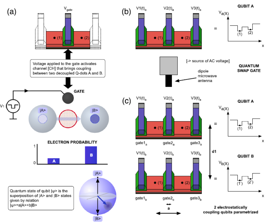
Two electrons on two separated single-electron lines tends to be in anti-correlated positions due to repulsion force as depicted in Fig.1.
In such a way we encounter the situation of two electrons placed on two different left (right) quantum dots with probabilities | ξ 1 ( t ) | 2 superscript subscript 𝜉 1 𝑡 2 |\xi_{1}(t)|^{2} | ξ 4 ( t ) | 2 superscript subscript 𝜉 4 𝑡 2 |\xi_{4}(t)|^{2} | ξ 2 ( t ) | 2 superscript subscript 𝜉 2 𝑡 2 |\xi_{2}(t)|^{2} | ξ 3 ( t ) | 2 superscript subscript 𝜉 3 𝑡 2 |\xi_{3}(t)|^{2} | ξ 1 ( t ) | 2 + . . + | ξ 4 ( t ) | 2 = 1 |\xi_{1}(t)|^{2}+..+|\xi_{4}(t)|^{2}=1 [3 ] :
| ψ ⟩ = ξ 1 ( t ) | 0 ⟩ A | 0 ⟩ B + ξ 2 ( t ) | 0 ⟩ A | 1 ⟩ B + ξ 3 ( t ) | 1 ⟩ A | 0 ⟩ B + ξ 4 ( t ) | 1 ⟩ A | 1 ⟩ B . ket 𝜓 subscript 𝜉 1 𝑡 subscript ket 0 𝐴 subscript ket 0 𝐵 subscript 𝜉 2 𝑡 subscript ket 0 𝐴 subscript ket 1 𝐵 subscript 𝜉 3 𝑡 subscript ket 1 𝐴 subscript ket 0 𝐵 subscript 𝜉 4 𝑡 subscript ket 1 𝐴 subscript ket 1 𝐵 \displaystyle\ket{\psi}=\xi_{1}(t)\ket{0}_{A}\ket{0}_{B}+\xi_{2}(t)\ket{0}_{A}\ket{1}_{B}+\xi_{3}(t)\ket{1}_{A}\ket{0}_{B}+\xi_{4}(t)\ket{1}_{A}\ket{1}_{B}. (6)
In case of 2 Single-Electron Lines we can write the effective Hamiltonian to be of the form
H ^ A − B = H ^ A × I ^ B + I ^ A × H ^ B + H ^ C o u l o m b : A − B = subscript ^ 𝐻 𝐴 𝐵 subscript ^ 𝐻 𝐴 subscript ^ 𝐼 𝐵 subscript ^ 𝐼 𝐴 subscript ^ 𝐻 𝐵 subscript ^ 𝐻 : 𝐶 𝑜 𝑢 𝑙 𝑜 𝑚 𝑏 𝐴 𝐵 absent \displaystyle\hat{H}_{A-B}=\hat{H}_{A}\times\hat{I}_{B}+\hat{I}_{A}\times\hat{H}_{B}+\hat{H}_{Coulomb:A-B}=
= ( E p 1 A | w L , A ⟩ ⟨ w L , A | + E p 2 A | w R , A ⟩ ⟨ w R , A | + t s 12 A | w R , A ⟩ ⟨ w L , A | + t s 21 A | w L , A ⟩ ⟨ w R , A | ) × I ^ B + absent limit-from subscript 𝐸 𝑝 1 𝐴 ket subscript 𝑤 𝐿 𝐴
bra subscript 𝑤 𝐿 𝐴
subscript 𝐸 𝑝 2 𝐴 ket subscript 𝑤 𝑅 𝐴
bra subscript 𝑤 𝑅 𝐴
subscript 𝑡 𝑠 12 𝐴 ket subscript 𝑤 𝑅 𝐴
bra subscript 𝑤 𝐿 𝐴
subscript 𝑡 𝑠 21 𝐴 ket subscript 𝑤 𝐿 𝐴
bra subscript 𝑤 𝑅 𝐴
subscript ^ 𝐼 𝐵 \displaystyle=(E_{p1A}\ket{w_{L,A}}\bra{w_{L,A}}+E_{p2A}\ket{w_{R,A}}\bra{w_{R,A}}+t_{s12A}\ket{w_{R,A}}\bra{w_{L,A}}+t_{s21A}\ket{w_{L,A}}\bra{w_{R,A}})\times\hat{I}_{B}+
+ I ^ A × ( E p 1 B | w L , B ⟩ ⟨ w L , B | + E p 2 B | w R , B ⟩ ⟨ w R , B | + t s 12 B | w R , B ⟩ ⟨ w L , B | + t s 21 B | w L , B ⟩ ⟨ w R , B | ) + limit-from subscript ^ 𝐼 𝐴 subscript 𝐸 𝑝 1 𝐵 ket subscript 𝑤 𝐿 𝐵
bra subscript 𝑤 𝐿 𝐵
subscript 𝐸 𝑝 2 𝐵 ket subscript 𝑤 𝑅 𝐵
bra subscript 𝑤 𝑅 𝐵
subscript 𝑡 𝑠 12 𝐵 ket subscript 𝑤 𝑅 𝐵
bra subscript 𝑤 𝐿 𝐵
subscript 𝑡 𝑠 21 𝐵 ket subscript 𝑤 𝐿 𝐵
bra subscript 𝑤 𝑅 𝐵
\displaystyle+\hat{I}_{A}\times(E_{p1B}\ket{w_{L,B}}\bra{w_{L,B}}+E_{p2B}\ket{w_{R,B}}\bra{w_{R,B}}+t_{s12B}\ket{w_{R,B}}\bra{w_{L,B}}+t_{s21B}\ket{w_{L,B}}\bra{w_{R,B}})+
+ [ q 1 | w L , A ⟩ | w L , B ⟩ ⟨ w L , A | ⟨ w L , B | + q 2 | w L , A ⟩ | w L , B ⟩ ⟨ w R , A | ⟨ w R , B | + q 3 | w L , A ⟩ | w L , B ⟩ ⟨ w R , A | ⟨ w R , B | + \displaystyle+\Bigg{[}q_{1}\ket{w_{L,A}}\ket{w_{L,B}}\bra{w_{L,A}}\bra{w_{L,B}}+q_{2}\ket{w_{L,A}}\ket{w_{L,B}}\bra{w_{R,A}}\bra{w_{R,B}}+q_{3}\ket{w_{L,A}}\ket{w_{L,B}}\bra{w_{R,A}}\bra{w_{R,B}}+
+ q 4 | w R , A ⟩ | w R , B ⟩ ⟨ w R , A | ⟨ w R , B | ] C o u l o m b \displaystyle+q_{4}\ket{w_{R,A}}\ket{w_{R,B}}\bra{w_{R,A}}\bra{w_{R,B}}\Bigg{]}_{Coulomb} (7)
Finally we obtain validation of tight-binding model in terms of Schrödinger equation, so we end up with following effective Hamiltonian
H ^ = ^ 𝐻 absent \displaystyle\hat{H}=
( E 1 a c o s ( Θ A ) 2 + E 2 a s i n ( Θ A ) 2 ( E 2 b − E 1 b ) 1 2 s i n ( 2 Θ B ) ( E 2 a − E 1 a ) 1 2 s i n ( 2 Θ A ) 0 ( E 2 b − E 1 b ) 1 2 s i n ( 2 Θ B ) E 1 a c o s ( Θ A ) 2 + E 2 a s i n ( Θ A ) 2 0 ( E 2 a − E 1 a ) 1 2 s i n ( 2 Θ A ) ( E 2 a − E 1 a ) 1 2 s i n ( 2 Θ A ) 0 E 1 a s i n ( Θ A ) 2 + E 2 a c o s ( Θ A ) 2 ( E 2 b − E 1 b ) 1 2 s i n ( 2 Θ B ) 0 ( E 2 a − E 1 a ) 1 2 s i n ( 2 Θ A ) ( E 2 b − E 1 b ) 1 2 s i n ( 2 Θ B ) E 1 a s i n ( Θ A ) 2 + E 2 a c o s ( Θ A ) 2 ) + limit-from matrix subscript 𝐸 1 𝑎 𝑐 𝑜 𝑠 superscript subscript Θ 𝐴 2 subscript 𝐸 2 𝑎 𝑠 𝑖 𝑛 superscript subscript Θ 𝐴 2 subscript 𝐸 2 𝑏 subscript 𝐸 1 𝑏 1 2 𝑠 𝑖 𝑛 2 subscript Θ 𝐵 subscript 𝐸 2 𝑎 subscript 𝐸 1 𝑎 1 2 𝑠 𝑖 𝑛 2 subscript Θ 𝐴 0 subscript 𝐸 2 𝑏 subscript 𝐸 1 𝑏 1 2 𝑠 𝑖 𝑛 2 subscript Θ 𝐵 subscript 𝐸 1 𝑎 𝑐 𝑜 𝑠 superscript subscript Θ 𝐴 2 subscript 𝐸 2 𝑎 𝑠 𝑖 𝑛 superscript subscript Θ 𝐴 2 0 subscript 𝐸 2 𝑎 subscript 𝐸 1 𝑎 1 2 𝑠 𝑖 𝑛 2 subscript Θ 𝐴 subscript 𝐸 2 𝑎 subscript 𝐸 1 𝑎 1 2 𝑠 𝑖 𝑛 2 subscript Θ 𝐴 0 subscript 𝐸 1 𝑎 𝑠 𝑖 𝑛 superscript subscript Θ 𝐴 2 subscript 𝐸 2 𝑎 𝑐 𝑜 𝑠 superscript subscript Θ 𝐴 2 subscript 𝐸 2 𝑏 subscript 𝐸 1 𝑏 1 2 𝑠 𝑖 𝑛 2 subscript Θ 𝐵 0 subscript 𝐸 2 𝑎 subscript 𝐸 1 𝑎 1 2 𝑠 𝑖 𝑛 2 subscript Θ 𝐴 subscript 𝐸 2 𝑏 subscript 𝐸 1 𝑏 1 2 𝑠 𝑖 𝑛 2 subscript Θ 𝐵 subscript 𝐸 1 𝑎 𝑠 𝑖 𝑛 superscript subscript Θ 𝐴 2 subscript 𝐸 2 𝑎 𝑐 𝑜 𝑠 superscript subscript Θ 𝐴 2 \displaystyle\begin{pmatrix}E_{1a}cos(\Theta_{A})^{2}+E_{2a}sin(\Theta_{A})^{2}&(E_{2b}-E_{1b})\frac{1}{2}sin(2\Theta_{B})&(E_{2a}-E_{1a})\frac{1}{2}sin(2\Theta_{A})&0\\
(E_{2b}-E_{1b})\frac{1}{2}sin(2\Theta_{B})&E_{1a}cos(\Theta_{A})^{2}+E_{2a}sin(\Theta_{A})^{2}&0&(E_{2a}-E_{1a})\frac{1}{2}sin(2\Theta_{A})\\
(E_{2a}-E_{1a})\frac{1}{2}sin(2\Theta_{A})&0&E_{1a}sin(\Theta_{A})^{2}+E_{2a}cos(\Theta_{A})^{2}&(E_{2b}-E_{1b})\frac{1}{2}sin(2\Theta_{B})\\
0&(E_{2a}-E_{1a})\frac{1}{2}sin(2\Theta_{A})&(E_{2b}-E_{1b})\frac{1}{2}sin(2\Theta_{B})&E_{1a}sin(\Theta_{A})^{2}+E_{2a}cos(\Theta_{A})^{2}\\
\end{pmatrix}+
( E 1 b c o s ( Θ B ) 2 + E 2 b s i n ( Θ B ) 2 0 0 0 0 E 1 b s i n ( Θ B ) 2 + E 2 b c o s ( Θ B ) 2 0 0 0 0 E 1 b c o s ( Θ B ) 2 + E 2 b s i n ( Θ B ) 2 0 0 0 0 E 1 b s i n ( Θ B ) 2 + E 2 b c o s ( Θ B ) 2 ) + limit-from matrix subscript 𝐸 1 𝑏 𝑐 𝑜 𝑠 superscript subscript Θ 𝐵 2 subscript 𝐸 2 𝑏 𝑠 𝑖 𝑛 superscript subscript Θ 𝐵 2 0 0 0 0 subscript 𝐸 1 𝑏 𝑠 𝑖 𝑛 superscript subscript Θ 𝐵 2 subscript 𝐸 2 𝑏 𝑐 𝑜 𝑠 superscript subscript Θ 𝐵 2 0 0 0 0 subscript 𝐸 1 𝑏 𝑐 𝑜 𝑠 superscript subscript Θ 𝐵 2 subscript 𝐸 2 𝑏 𝑠 𝑖 𝑛 superscript subscript Θ 𝐵 2 0 0 0 0 subscript 𝐸 1 𝑏 𝑠 𝑖 𝑛 superscript subscript Θ 𝐵 2 subscript 𝐸 2 𝑏 𝑐 𝑜 𝑠 superscript subscript Θ 𝐵 2 \displaystyle\begin{pmatrix}E_{1b}cos(\Theta_{B})^{2}+E_{2b}sin(\Theta_{B})^{2}&0&0&0\\
0&E_{1b}sin(\Theta_{B})^{2}+E_{2b}cos(\Theta_{B})^{2}&0&0\\
0&0&E_{1b}cos(\Theta_{B})^{2}+E_{2b}sin(\Theta_{B})^{2}&0\\
0&0&0&E_{1b}sin(\Theta_{B})^{2}+E_{2b}cos(\Theta_{B})^{2}\end{pmatrix}+
+ ( q 1 0 0 0 0 q 2 0 0 0 0 q 3 0 0 0 0 q 4 ) matrix subscript 𝑞 1 0 0 0 0 subscript 𝑞 2 0 0 0 0 subscript 𝑞 3 0 0 0 0 subscript 𝑞 4 \displaystyle+\begin{pmatrix}q_{1}&0&0&0\\
0&q_{2}&0&0\\
0&0&q_{3}&0\\
0&0&0&q_{4}\end{pmatrix} (8)
where 4 terms are responsible for 2 qubits being at a distance d mutual Coulomb interaction (as depicted in Fig.1.) and given as
q 1 = ∫ − ∞ + ∞ ∫ − ∞ + ∞ d x A d x B e 2 4 π ϵ 0 d 2 + ( x A − x B ) 2 | c o s ( Θ A ) ψ E 1 ( x A ) + s i n ( Θ A ) ψ E 2 ( x A ) | 2 ∗ | c o s ( Θ B ) ψ E 1 ( x B ) + s i n ( Θ B ) ψ E 2 ( x B ) | 2 subscript 𝑞 1 superscript subscript superscript subscript 𝑑 subscript 𝑥 𝐴 𝑑 subscript 𝑥 𝐵 superscript 𝑒 2 4 𝜋 subscript italic-ϵ 0 superscript 𝑑 2 superscript subscript 𝑥 𝐴 subscript 𝑥 𝐵 2 superscript 𝑐 𝑜 𝑠 subscript Θ 𝐴 subscript 𝜓 𝐸 1 subscript 𝑥 𝐴 𝑠 𝑖 𝑛 subscript Θ 𝐴 subscript 𝜓 𝐸 2 subscript 𝑥 𝐴 2 superscript 𝑐 𝑜 𝑠 subscript Θ 𝐵 subscript 𝜓 𝐸 1 subscript 𝑥 𝐵 𝑠 𝑖 𝑛 subscript Θ 𝐵 subscript 𝜓 𝐸 2 subscript 𝑥 𝐵 2 \displaystyle q_{1}=\int_{-\infty}^{+\infty}\int_{-\infty}^{+\infty}\frac{dx_{A}dx_{B}e^{2}}{4\pi\epsilon_{0}\sqrt{d^{2}+(x_{A}-x_{B})^{2}}}|cos(\Theta_{A})\psi_{E1}(x_{A})+sin(\Theta_{A})\psi_{E2}(x_{A})|^{2}*|cos(\Theta_{B})\psi_{E1}(x_{B})+sin(\Theta_{B})\psi_{E2}(x_{B})|^{2} (9)
q 2 = ∫ − ∞ + ∞ ∫ − ∞ + ∞ d x A d x B e 2 4 π ϵ 0 d 2 + ( x A − x B ) 2 | c o s ( Θ A ) ψ E 1 ( x A ) + s i n ( Θ A ) ψ E 2 ( x A ) | 2 ∗ | − s i n ( Θ B ) ψ E 1 ( x B ) + c o s ( Θ B ) ψ E 2 ( x B ) | 2 subscript 𝑞 2 superscript subscript superscript subscript 𝑑 subscript 𝑥 𝐴 𝑑 subscript 𝑥 𝐵 superscript 𝑒 2 4 𝜋 subscript italic-ϵ 0 superscript 𝑑 2 superscript subscript 𝑥 𝐴 subscript 𝑥 𝐵 2 superscript 𝑐 𝑜 𝑠 subscript Θ 𝐴 subscript 𝜓 𝐸 1 subscript 𝑥 𝐴 𝑠 𝑖 𝑛 subscript Θ 𝐴 subscript 𝜓 𝐸 2 subscript 𝑥 𝐴 2 superscript 𝑠 𝑖 𝑛 subscript Θ 𝐵 subscript 𝜓 𝐸 1 subscript 𝑥 𝐵 𝑐 𝑜 𝑠 subscript Θ 𝐵 subscript 𝜓 𝐸 2 subscript 𝑥 𝐵 2 \displaystyle q_{2}=\int_{-\infty}^{+\infty}\int_{-\infty}^{+\infty}\frac{dx_{A}dx_{B}e^{2}}{4\pi\epsilon_{0}\sqrt{d^{2}+(x_{A}-x_{B})^{2}}}|cos(\Theta_{A})\psi_{E1}(x_{A})+sin(\Theta_{A})\psi_{E2}(x_{A})|^{2}*|-sin(\Theta_{B})\psi_{E1}(x_{B})+cos(\Theta_{B})\psi_{E2}(x_{B})|^{2} (10)
q 3 = ∫ − ∞ + ∞ ∫ − ∞ + ∞ d x A d x B e 2 4 π ϵ 0 d 2 + ( x A − x B ) 2 | − s i n ( Θ A ) ψ E 1 ( x A ) + c o s ( Θ A ) ψ E 2 ( x A ) | 2 ∗ | c o s ( Θ B ) ψ E 1 ( x B ) + s i n ( Θ B ) ψ E 2 ( x B ) | 2 subscript 𝑞 3 superscript subscript superscript subscript 𝑑 subscript 𝑥 𝐴 𝑑 subscript 𝑥 𝐵 superscript 𝑒 2 4 𝜋 subscript italic-ϵ 0 superscript 𝑑 2 superscript subscript 𝑥 𝐴 subscript 𝑥 𝐵 2 superscript 𝑠 𝑖 𝑛 subscript Θ 𝐴 subscript 𝜓 𝐸 1 subscript 𝑥 𝐴 𝑐 𝑜 𝑠 subscript Θ 𝐴 subscript 𝜓 𝐸 2 subscript 𝑥 𝐴 2 superscript 𝑐 𝑜 𝑠 subscript Θ 𝐵 subscript 𝜓 𝐸 1 subscript 𝑥 𝐵 𝑠 𝑖 𝑛 subscript Θ 𝐵 subscript 𝜓 𝐸 2 subscript 𝑥 𝐵 2 \displaystyle q_{3}=\int_{-\infty}^{+\infty}\int_{-\infty}^{+\infty}\frac{dx_{A}dx_{B}e^{2}}{4\pi\epsilon_{0}\sqrt{d^{2}+(x_{A}-x_{B})^{2}}}|-sin(\Theta_{A})\psi_{E1}(x_{A})+cos(\Theta_{A})\psi_{E2}(x_{A})|^{2}*|cos(\Theta_{B})\psi_{E1}(x_{B})+sin(\Theta_{B})\psi_{E2}(x_{B})|^{2} (11)
q 4 = ∫ − ∞ + ∞ ∫ − ∞ + ∞ d x A d x B e 2 4 π ϵ 0 d 2 + ( x A − x B ) 2 | − s i n ( Θ A ) ψ E 1 ( x A ) + c o s ( Θ A ) ψ E 2 ( x A ) | 2 | − s i n ( Θ B ) ψ E 1 ( x B ) + c o s ( Θ B ) ψ E 2 ( x B ) | 2 . subscript 𝑞 4 superscript subscript superscript subscript 𝑑 subscript 𝑥 𝐴 𝑑 subscript 𝑥 𝐵 superscript 𝑒 2 4 𝜋 subscript italic-ϵ 0 superscript 𝑑 2 superscript subscript 𝑥 𝐴 subscript 𝑥 𝐵 2 superscript 𝑠 𝑖 𝑛 subscript Θ 𝐴 subscript 𝜓 𝐸 1 subscript 𝑥 𝐴 𝑐 𝑜 𝑠 subscript Θ 𝐴 subscript 𝜓 𝐸 2 subscript 𝑥 𝐴 2 superscript 𝑠 𝑖 𝑛 subscript Θ 𝐵 subscript 𝜓 𝐸 1 subscript 𝑥 𝐵 𝑐 𝑜 𝑠 subscript Θ 𝐵 subscript 𝜓 𝐸 2 subscript 𝑥 𝐵 2 \displaystyle q_{4}=\int_{-\infty}^{+\infty}\int_{-\infty}^{+\infty}\frac{dx_{A}dx_{B}e^{2}}{4\pi\epsilon_{0}\sqrt{d^{2}+(x_{A}-x_{B})^{2}}}|-sin(\Theta_{A})\psi_{E1}(x_{A})+cos(\Theta_{A})\psi_{E2}(x_{A})|^{2}|-sin(\Theta_{B})\psi_{E1}(x_{B})+cos(\Theta_{B})\psi_{E2}(x_{B})|^{2}.
In first approximation we consider two-position based qubits as non-interacting and slightly perturbed by electrostatic single-electron to single-electron interaction
what naturally leads to first approximation of system eigenstate as tensor product of two Hilbert spaces belonging to each qubits in the form as given below:
| ψ ⟩ E n e r g y , A − B = ( γ E 1 A γ E 2 A ) × ( γ E 1 B γ E 2 B ) = ( γ E 1 A γ E 1 B = c o s ( ξ A ) e i ϕ E 1 A c o s ( ξ B ) e i ϕ E 1 B γ E 1 A γ E 2 B = c o s ( ξ A ) e i ϕ E 1 A s i n ( ξ B ) e i ϕ E 2 B γ E 2 A γ E 1 B = s i n ( ξ A ) e i ϕ E 2 A c o s ( ξ B ) e i ϕ E 1 B γ E 2 A γ E 2 B = s i n ( ξ A ) e i ϕ E 2 A s i n ( ξ B ) e i ϕ E 2 B ) . subscript ket 𝜓 𝐸 𝑛 𝑒 𝑟 𝑔 𝑦 𝐴 𝐵
matrix subscript 𝛾 𝐸 1 𝐴 subscript 𝛾 𝐸 2 𝐴 matrix subscript 𝛾 𝐸 1 𝐵 subscript 𝛾 𝐸 2 𝐵 matrix subscript 𝛾 𝐸 1 𝐴 subscript 𝛾 𝐸 1 𝐵 𝑐 𝑜 𝑠 subscript 𝜉 𝐴 superscript 𝑒 𝑖 subscript italic-ϕ 𝐸 1 𝐴 𝑐 𝑜 𝑠 subscript 𝜉 𝐵 superscript 𝑒 𝑖 subscript italic-ϕ 𝐸 1 𝐵 subscript 𝛾 𝐸 1 𝐴 subscript 𝛾 𝐸 2 𝐵 𝑐 𝑜 𝑠 subscript 𝜉 𝐴 superscript 𝑒 𝑖 subscript italic-ϕ 𝐸 1 𝐴 𝑠 𝑖 𝑛 subscript 𝜉 𝐵 superscript 𝑒 𝑖 subscript italic-ϕ 𝐸 2 𝐵 subscript 𝛾 𝐸 2 𝐴 subscript 𝛾 𝐸 1 𝐵 𝑠 𝑖 𝑛 subscript 𝜉 𝐴 superscript 𝑒 𝑖 subscript italic-ϕ 𝐸 2 𝐴 𝑐 𝑜 𝑠 subscript 𝜉 𝐵 superscript 𝑒 𝑖 subscript italic-ϕ 𝐸 1 𝐵 subscript 𝛾 𝐸 2 𝐴 subscript 𝛾 𝐸 2 𝐵 𝑠 𝑖 𝑛 subscript 𝜉 𝐴 superscript 𝑒 𝑖 subscript italic-ϕ 𝐸 2 𝐴 𝑠 𝑖 𝑛 subscript 𝜉 𝐵 superscript 𝑒 𝑖 subscript italic-ϕ 𝐸 2 𝐵 \displaystyle\ket{\psi}_{Energy,A-B}=\begin{pmatrix}\gamma_{E1A}\\
\gamma_{E2A}\\
\end{pmatrix}\times\begin{pmatrix}\gamma_{E1B}\\
\gamma_{E2B}\\
\end{pmatrix}=\begin{pmatrix}\gamma_{E1A}\gamma_{E1B}=cos(\xi_{A})e^{i\phi_{E1A}}cos(\xi_{B})e^{i\phi_{E1B}}\\
\gamma_{E1A}\gamma_{E2B}=cos(\xi_{A})e^{i\phi_{E1A}}sin(\xi_{B})e^{i\phi_{E2B}}\\
\gamma_{E2A}\gamma_{E1B}=sin(\xi_{A})e^{i\phi_{E2A}}cos(\xi_{B})e^{i\phi_{E1B}}\\
\gamma_{E2A}\gamma_{E2B}=sin(\xi_{A})e^{i\phi_{E2A}}sin(\xi_{B})e^{i\phi_{E2B}}\\
\end{pmatrix}. (13)
Search for system ground state naturally implies minimization of Coulomb energy as criteria for lowest energy state that can be expressed by proper self-alignment of electrons in anticorrelated way and thus leading to minimization of Coulomb interaction energy. Coulomb energy is given as
E c ( ξ A , ξ B ) = ⟨ ψ | H ^ c | ψ ⟩ = subscript 𝐸 𝑐 subscript 𝜉 𝐴 subscript 𝜉 𝐵 bra 𝜓 subscript ^ 𝐻 𝑐 ket 𝜓 absent \displaystyle E_{c}(\xi_{A},\xi_{B})=\bra{\psi}\hat{H}_{c}\ket{\psi}=
= q 1 c o s ( ξ A ) 2 c o s ( ξ B ) 2 + q 2 c o s ( ξ A ) 2 s i n ( ξ B ) 2 + q 3 s i n ( ξ A ) 2 c o s ( ξ B ) 2 + q 4 s i n ( ξ A ) 2 s i n ( ξ B ) 2 . absent subscript 𝑞 1 𝑐 𝑜 𝑠 superscript subscript 𝜉 𝐴 2 𝑐 𝑜 𝑠 superscript subscript 𝜉 𝐵 2 subscript 𝑞 2 𝑐 𝑜 𝑠 superscript subscript 𝜉 𝐴 2 𝑠 𝑖 𝑛 superscript subscript 𝜉 𝐵 2 subscript 𝑞 3 𝑠 𝑖 𝑛 superscript subscript 𝜉 𝐴 2 𝑐 𝑜 𝑠 superscript subscript 𝜉 𝐵 2 subscript 𝑞 4 𝑠 𝑖 𝑛 superscript subscript 𝜉 𝐴 2 𝑠 𝑖 𝑛 superscript subscript 𝜉 𝐵 2 \displaystyle=q_{1}cos(\xi_{A})^{2}cos(\xi_{B})^{2}+q_{2}cos(\xi_{A})^{2}sin(\xi_{B})^{2}+q_{3}sin(\xi_{A})^{2}cos(\xi_{B})^{2}+q_{4}sin(\xi_{A})^{2}sin(\xi_{B})^{2}. (14)
Coulomb energy minimization condition brings following constrains
d d ξ A E c ( ξ A , ξ B ) = 0 , d d ξ B E c ( ξ A , ξ B ) = 0 , formulae-sequence 𝑑 𝑑 subscript 𝜉 𝐴 subscript 𝐸 𝑐 subscript 𝜉 𝐴 subscript 𝜉 𝐵 0 𝑑 𝑑 subscript 𝜉 𝐵 subscript 𝐸 𝑐 subscript 𝜉 𝐴 subscript 𝜉 𝐵 0 \displaystyle\frac{d}{d\xi_{A}}E_{c}(\xi_{A},\xi_{B})=0,\frac{d}{d\xi_{B}}E_{c}(\xi_{A},\xi_{B})=0, (15)
and hence we have
0 = d d ξ A E c ( ξ A , ξ B ) = 2 ( − s i n ( ξ A ) [ q 1 c o s ( ξ B ) 2 + q 2 s i n ( ξ B ) 2 ] + \displaystyle 0=\frac{d}{d\xi_{A}}E_{c}(\xi_{A},\xi_{B})=2(-sin(\xi_{A})[q_{1}cos(\xi_{B})^{2}+q_{2}sin(\xi_{B})^{2}]+
+ c o s ( ξ A ) [ q 3 c o s ( ξ B ) 2 + q 4 s i n ( ξ B ) 2 ] ) , \displaystyle+cos(\xi_{A})[q_{3}cos(\xi_{B})^{2}+q_{4}sin(\xi_{B})^{2}]), (16)
that leads to
t a n ( ξ A ) = [ q 3 c o s ( ξ B ) 2 + q 4 s i n ( ξ B ) 2 ] [ q 1 c o s ( ξ B ) 2 + q 2 s i n ( ξ B ) 2 ] = [ q 3 + q 4 t a n ( ξ B ) 2 ] [ q 1 + q 2 t a n ( ξ B ) 2 ] . 𝑡 𝑎 𝑛 subscript 𝜉 𝐴 delimited-[] subscript 𝑞 3 𝑐 𝑜 𝑠 superscript subscript 𝜉 𝐵 2 subscript 𝑞 4 𝑠 𝑖 𝑛 superscript subscript 𝜉 𝐵 2 delimited-[] subscript 𝑞 1 𝑐 𝑜 𝑠 superscript subscript 𝜉 𝐵 2 subscript 𝑞 2 𝑠 𝑖 𝑛 superscript subscript 𝜉 𝐵 2 delimited-[] subscript 𝑞 3 subscript 𝑞 4 𝑡 𝑎 𝑛 superscript subscript 𝜉 𝐵 2 delimited-[] subscript 𝑞 1 subscript 𝑞 2 𝑡 𝑎 𝑛 superscript subscript 𝜉 𝐵 2 \displaystyle tan(\xi_{A})=\frac{[q_{3}cos(\xi_{B})^{2}+q_{4}sin(\xi_{B})^{2}]}{[q_{1}cos(\xi_{B})^{2}+q_{2}sin(\xi_{B})^{2}]}=\frac{[q_{3}+q_{4}tan(\xi_{B})^{2}]}{[q_{1}+q_{2}tan(\xi_{B})^{2}]}. (17)
Now we exercise second constrain on energy minimization what brings
0 = d d ξ B E c ( ξ A , ξ B ) = 2 ( + c o s ( ξ A ) 2 [ − q 1 s i n ( ξ B ) + q 2 c o s ( ξ B ) ] + \displaystyle 0=\frac{d}{d\xi_{B}}E_{c}(\xi_{A},\xi_{B})=2(+cos(\xi_{A})^{2}[-q_{1}sin(\xi_{B})+q_{2}cos(\xi_{B})]+
+ s i n ( ξ A ) 2 [ − q 3 s i n ( ξ B ) + q 4 c o s ( ξ B ) ] ) , \displaystyle+sin(\xi_{A})^{2}[-q_{3}sin(\xi_{B})+q_{4}cos(\xi_{B})]), (18)
and we obtain
t a n ( ξ A ) 2 = [ − q 1 s i n ( ξ B ) + q 2 c o s ( ξ B ) ] [ q 3 s i n ( ξ B ) − q 4 c o s ( ξ B ) ] = [ q 3 c o s ( ξ B ) 2 + q 4 s i n ( ξ B ) 2 ] 2 [ q 1 c o s ( ξ B ) 2 + q 2 s i n ( ξ B ) 2 ] 2 . 𝑡 𝑎 𝑛 superscript subscript 𝜉 𝐴 2 delimited-[] subscript 𝑞 1 𝑠 𝑖 𝑛 subscript 𝜉 𝐵 subscript 𝑞 2 𝑐 𝑜 𝑠 subscript 𝜉 𝐵 delimited-[] subscript 𝑞 3 𝑠 𝑖 𝑛 subscript 𝜉 𝐵 subscript 𝑞 4 𝑐 𝑜 𝑠 subscript 𝜉 𝐵 superscript delimited-[] subscript 𝑞 3 𝑐 𝑜 𝑠 superscript subscript 𝜉 𝐵 2 subscript 𝑞 4 𝑠 𝑖 𝑛 superscript subscript 𝜉 𝐵 2 2 superscript delimited-[] subscript 𝑞 1 𝑐 𝑜 𝑠 superscript subscript 𝜉 𝐵 2 subscript 𝑞 2 𝑠 𝑖 𝑛 superscript subscript 𝜉 𝐵 2 2 \displaystyle tan(\xi_{A})^{2}=\frac{[-q_{1}sin(\xi_{B})+q_{2}cos(\xi_{B})]}{[q_{3}sin(\xi_{B})-q_{4}cos(\xi_{B})]}=\frac{[q_{3}cos(\xi_{B})^{2}+q_{4}sin(\xi_{B})^{2}]^{2}}{[q_{1}cos(\xi_{B})^{2}+q_{2}sin(\xi_{B})^{2}]^{2}}. (19)
Under assumption that qubit A is occupying 2 energy levels E 1 A subscript 𝐸 1 𝐴 E_{1A} E 2 A subscript 𝐸 2 𝐴 E_{2A} E 1 B subscript 𝐸 1 𝐵 E_{1B} E 2 B subscript 𝐸 2 𝐵 E_{2B}
t a n ( ξ A ) 2 = [ − q 1 t a n ( ξ B ) + q 2 ] [ q 3 t a n ( ξ B ) − q 4 ] = [ q 3 + q 4 t a n ( ξ B ) 2 ] 2 [ q 1 + q 2 t a n ( ξ B ) 2 ] 2 , 𝑡 𝑎 𝑛 superscript subscript 𝜉 𝐴 2 delimited-[] subscript 𝑞 1 𝑡 𝑎 𝑛 subscript 𝜉 𝐵 subscript 𝑞 2 delimited-[] subscript 𝑞 3 𝑡 𝑎 𝑛 subscript 𝜉 𝐵 subscript 𝑞 4 superscript delimited-[] subscript 𝑞 3 subscript 𝑞 4 𝑡 𝑎 𝑛 superscript subscript 𝜉 𝐵 2 2 superscript delimited-[] subscript 𝑞 1 subscript 𝑞 2 𝑡 𝑎 𝑛 superscript subscript 𝜉 𝐵 2 2 \displaystyle tan(\xi_{A})^{2}=\frac{[-q_{1}tan(\xi_{B})+q_{2}]}{[q_{3}tan(\xi_{B})-q_{4}]}=\frac{[q_{3}+q_{4}tan(\xi_{B})^{2}]^{2}}{[q_{1}+q_{2}tan(\xi_{B})^{2}]^{2}}, (20)
| γ E 1 A | 2 = c o s ( ξ A ) 2 = p E 1 A superscript subscript 𝛾 𝐸 1 𝐴 2 𝑐 𝑜 𝑠 superscript subscript 𝜉 𝐴 2 subscript 𝑝 𝐸 1 𝐴 |\gamma_{E1A}|^{2}=cos(\xi_{A})^{2}=p_{E1A} | γ E 2 A | 2 = c o s ( ξ A ) 2 = p E 1 A superscript subscript 𝛾 𝐸 2 𝐴 2 𝑐 𝑜 𝑠 superscript subscript 𝜉 𝐴 2 subscript 𝑝 𝐸 1 𝐴 |\gamma_{E2A}|^{2}=cos(\xi_{A})^{2}=p_{E1A} | γ E 1 B | 2 = c o s ( ξ B ) 2 = p E 1 B superscript subscript 𝛾 𝐸 1 𝐵 2 𝑐 𝑜 𝑠 superscript subscript 𝜉 𝐵 2 subscript 𝑝 𝐸 1 𝐵 |\gamma_{E1B}|^{2}=cos(\xi_{B})^{2}=p_{E1B} | γ E 2 B | 2 = s i n ( ξ B ) 2 = p E 2 B superscript subscript 𝛾 𝐸 2 𝐵 2 𝑠 𝑖 𝑛 superscript subscript 𝜉 𝐵 2 subscript 𝑝 𝐸 2 𝐵 |\gamma_{E2B}|^{2}=sin(\xi_{B})^{2}=p_{E2B} q 1 subscript 𝑞 1 q_{1} q 2 subscript 𝑞 2 q_{2} q 3 subscript 𝑞 3 q_{3} q 4 subscript 𝑞 4 q_{4} ( r A (r_{A} r A subscript 𝑟 𝐴 r_{A} 3 Θ A , Θ B subscript Θ 𝐴 subscript Θ 𝐵
\Theta_{A},\Theta_{B} q 1 subscript 𝑞 1 q_{1} q 4 subscript 𝑞 4 q_{4} ( E 1 A , E 2 A ) subscript 𝐸 1 𝐴 subscript 𝐸 2 𝐴 (E_{1A},E_{2A}) ( E 1 B , E 2 B ) subscript 𝐸 1 𝐵 subscript 𝐸 2 𝐵 (E_{1B},E_{2B})
Figure 1: Case of position based qubit encoded in system of two coupled quantum dot controlled electrostatically and case of simple Quantum Swap Gate [6 ] .
III Conclusions
It is quite straightforward to generalize the system under the consideration of the case of N perturbatively electrostatically interacting position based qubits described by Wannier functions. Those qubits can be further subjected to Rabi oscillations by local microwave fields acting on qubits in their direct proximity which might imply evolution of the system ground state with time.
H ^ A − B = H ^ A × I ^ B + I ^ A × H ^ B + H ^ C o u l o m b : A − B = subscript ^ 𝐻 𝐴 𝐵 subscript ^ 𝐻 𝐴 subscript ^ 𝐼 𝐵 subscript ^ 𝐼 𝐴 subscript ^ 𝐻 𝐵 subscript ^ 𝐻 : 𝐶 𝑜 𝑢 𝑙 𝑜 𝑚 𝑏 𝐴 𝐵 absent \displaystyle\hat{H}_{A-B}=\hat{H}_{A}\times\hat{I}_{B}+\hat{I}_{A}\times\hat{H}_{B}+\hat{H}_{Coulomb:A-B}=
= ( E p 1 A | w L , A ⟩ ⟨ w L , A | + E p 2 A | w R , A ⟩ ⟨ w R , A | + t s 12 A | w R , A ⟩ ⟨ w L , A | + t s 21 A | w L , A ⟩ ⟨ w R , A | ) × I ^ B + absent limit-from subscript 𝐸 𝑝 1 𝐴 ket subscript 𝑤 𝐿 𝐴
bra subscript 𝑤 𝐿 𝐴
subscript 𝐸 𝑝 2 𝐴 ket subscript 𝑤 𝑅 𝐴
bra subscript 𝑤 𝑅 𝐴
subscript 𝑡 𝑠 12 𝐴 ket subscript 𝑤 𝑅 𝐴
bra subscript 𝑤 𝐿 𝐴
subscript 𝑡 𝑠 21 𝐴 ket subscript 𝑤 𝐿 𝐴
bra subscript 𝑤 𝑅 𝐴
subscript ^ 𝐼 𝐵 \displaystyle=(E_{p1A}\ket{w_{L,A}}\bra{w_{L,A}}+E_{p2A}\ket{w_{R,A}}\bra{w_{R,A}}+t_{s12A}\ket{w_{R,A}}\bra{w_{L,A}}+t_{s21A}\ket{w_{L,A}}\bra{w_{R,A}})\times\hat{I}_{B}+
+ I ^ A × ( E p 1 B | w L , B ⟩ ⟨ w L , B | + E p 2 B | w R , B ⟩ ⟨ w R , B | + t s 12 B | w R , B ⟩ ⟨ w L , B | + t s 21 B | w L , B ⟩ ⟨ w R , B | ) + limit-from subscript ^ 𝐼 𝐴 subscript 𝐸 𝑝 1 𝐵 ket subscript 𝑤 𝐿 𝐵
bra subscript 𝑤 𝐿 𝐵
subscript 𝐸 𝑝 2 𝐵 ket subscript 𝑤 𝑅 𝐵
bra subscript 𝑤 𝑅 𝐵
subscript 𝑡 𝑠 12 𝐵 ket subscript 𝑤 𝑅 𝐵
bra subscript 𝑤 𝐿 𝐵
subscript 𝑡 𝑠 21 𝐵 ket subscript 𝑤 𝐿 𝐵
bra subscript 𝑤 𝑅 𝐵
\displaystyle+\hat{I}_{A}\times(E_{p1B}\ket{w_{L,B}}\bra{w_{L,B}}+E_{p2B}\ket{w_{R,B}}\bra{w_{R,B}}+t_{s12B}\ket{w_{R,B}}\bra{w_{L,B}}+t_{s21B}\ket{w_{L,B}}\bra{w_{R,B}})+
+ [ q 1 | w L , A ⟩ | w L , B ⟩ ⟨ w L , A | ⟨ w L , B | + q 2 | w L , A ⟩ | w L , B ⟩ ⟨ w R , A | ⟨ w R , B | + q 3 | w L , A ⟩ | w L , B ⟩ ⟨ w R , A | ⟨ w R , B | + \displaystyle+\Bigg{[}q_{1}\ket{w_{L,A}}\ket{w_{L,B}}\bra{w_{L,A}}\bra{w_{L,B}}+q_{2}\ket{w_{L,A}}\ket{w_{L,B}}\bra{w_{R,A}}\bra{w_{R,B}}+q_{3}\ket{w_{L,A}}\ket{w_{L,B}}\bra{w_{R,A}}\bra{w_{R,B}}+
+ q 4 | w R , A ⟩ | w R , B ⟩ ⟨ w R , A | ⟨ w R , B | ] C o u l o m b + \displaystyle+q_{4}\ket{w_{R,A}}\ket{w_{R,B}}\bra{w_{R,A}}\bra{w_{R,B}}\Bigg{]}_{Coulomb}+
+ ∑ r , s , u , d ( | w L , A ⟩ ⟨ w L , A | + | w R , A ⟩ ⟨ w R , A | ) ( | w L , B ⟩ ⟨ w L , b | + | w R , B ⟩ ⟨ w R , B | ) subscript 𝑟 𝑠 𝑢 𝑑
ket subscript 𝑤 𝐿 𝐴
bra subscript 𝑤 𝐿 𝐴
ket subscript 𝑤 𝑅 𝐴
bra subscript 𝑤 𝑅 𝐴
ket subscript 𝑤 𝐿 𝐵
bra subscript 𝑤 𝐿 𝑏
ket subscript 𝑤 𝑅 𝐵
bra subscript 𝑤 𝑅 𝐵
\displaystyle+\sum_{r,s,u,d}(\ket{w_{L},A}\bra{w_{L},A}+\ket{w_{R},A}\bra{w_{R},A})(\ket{w_{L},B}\bra{w_{L},b}+\ket{w_{R},B}\bra{w_{R},B})
g ( t , r , s , u , d ) ( | E L , r ⟩ | E R , s ⟩ ) ( ⟨ E L , u | ⟨ E R , d | ) ( | w L , A ⟩ ⟨ w L , A | + | w R , A ⟩ ⟨ w R , A | ) ( | w L , B ⟩ ⟨ w L , b | + | w R , B ⟩ ⟨ w R , B | ) . 𝑔 𝑡 𝑟 𝑠 𝑢 𝑑 ket subscript 𝐸 𝐿 𝑟
ket subscript 𝐸 𝑅 𝑠
bra subscript 𝐸 𝐿 𝑢
bra subscript 𝐸 𝑅 𝑑
ket subscript 𝑤 𝐿 𝐴
bra subscript 𝑤 𝐿 𝐴
ket subscript 𝑤 𝑅 𝐴
bra subscript 𝑤 𝑅 𝐴
ket subscript 𝑤 𝐿 𝐵
bra subscript 𝑤 𝐿 𝑏
ket subscript 𝑤 𝑅 𝐵
bra subscript 𝑤 𝑅 𝐵
\displaystyle g(t,r,s,u,d)(\ket{E_{L,r}}\ket{E_{R,s}})(\bra{E_{L,u}}\bra{E_{R,d}})(\ket{w_{L},A}\bra{w_{L},A}+\ket{w_{R},A}\bra{w_{R},A})(\ket{w_{L},B}\bra{w_{L},b}+\ket{w_{R},B}\bra{w_{R},B}). (21)
It is quite straightforward to apply the presented scheme for the case of N position based qubits implementing various quantum gates [7 ] ,[8 ] .
Obtained results have its significance in quantum communication as well [9 ] .
References
[1]
A.R.Mills, D.M.Zajac, M.J.Gullans et al. , Shuttling a single charge across a one-dimensional array of silicon quantum dots , Nature Communication, Vol. 10, 2019.
[2]
T. Fujisawa, T. Hayashi, Y. Hirayama, H. D. Cheong, Y. H. Jeong, Electron counting of single-electron tunneling current ,
Applied Physical Letters, Vol. 84, 2004
[3]
K.Pomorski, P.Giounanlis, E.Blokhina, D.Leipold, R.B.Staszewski,
Analytic view on coupled single-electron lines , Semiconductor Science and Technology, Vol. 34, Nr 12, 2019
[4]
K.Pomorski, Electrostatically interacting Wannier qubits in curved space , Arxiv: 2112.13470v1, 2019.
[5]
K.Pomorski, Equivalence between finite state stochastic machine, non-dissipative and dissipative tight-binding and Schrödinger model ,
Mathematics and Computers in Simulation,
Vol. 209, 2023, Elsevier.
[6]
K.Pomorski, P.Peczkowski, R.B.Staszewski, Analytical solutions for N interacting electron system confined in graph of coupled electrostatic semiconductor and superconducting quantum dots in tight-binding model , Cryogenics, Vol. 109, 2020.
[7]
K.Pomorski, Analytic view on N body interaction in electrostatic quantum gates and decoherence effects in tight-binding model ,
Vol. 19, Issue 04, 2021, International Journal of Quantum Information
[8]
K.Pomorski, Analytical solutions for N-Electron interacting system confined in graph of coupled electrostatic semiconductor and superconducting quantum dots in tight-binding model with focus on quantum information processing , Springer Proceedings in Physics, Vol. 279, 2023
[9]
K.Pomorski, R.B.Staszewski, Towards quantum internet and non-local communication in position-based qubits ,
AIP Conf. Proc., 2241, 2020