Partial fraction expansions
and zeros of Hankel transforms
Abstract. It is proved by the method of partial fraction expansions and Sturm’s oscillation theory that the zeros of certain Hankel transforms are all real and distributed regularly between consecutive zeros of Bessel functions. As an application, the sufficient or necessary conditions on parameters for which hypergeometric functions belong to the Laguerre-Pólya class are investigated in a constructive manner.
Keywords. Bessel functions, Fourier transforms, Hankel transforms,
Laguerre-Pólya class, partial fraction expansions, transference principle.
2020 MSC. 30D10, 33C10, 34C10, 44A15.
1 Introduction
This paper deals with partial fraction expansions for the ratios of Hankel transforms to Bessel functions and its applications to the theory of zeros of Hankel transforms, which extend those analogous results of Hurwitz and Pólya [20] concerning Fourier cosine and sine transforms.
The Hankel transform under consideration is defined by
| (1.1) |
where stands for the Bessel function of the first kind of order . It will be assumed throughout that is real and In the special cases (1.1) reduces to
the Fourier cosine and sine transforms, respectively. It is shown by Hurwitz and Pólya [20] that the zeros of Fourier transforms of the above type are all real, simple and regularly distributed when is positive and increasing unless it is a step function with finitely many jumps at rational points.
In this paper we aim to investigate the nature and distribution of zeros of Hankel transforms. To describe briefly our methods and results, we shall derive a family of partial fraction expansions of the form
with parameter where denotes the positive zero of of rank and is preassigned to determine the residues explicitly. As it will become clearer in the sequel, a partial fraction expansion of this kind will enable us to locate each zero of between consecutive zeros of provided that keeps constant sign for all . In the particular case we shall employ a version of Sturm’s comparison theorems to find sufficient conditions on for to keep the same sign.
While it will be assumed implicitly that the principal branch of logarithm is taken in the definition of , it is convenient to introduce the kernel
| (1.2) |
and consider the normalized Hankel transform defined by
| (1.3) |
Due to the readily-verified relations
| (1.4) |
it is evident that Bessel functions share the zeros in common for and so do Hankel transforms A remarkable aspect of the normalized Hankel transform is that it belongs to the Laguerre-Pólya class of entire functions under the aforementioned sign-condition.
The Hankel transform of the present type (1.1) or (1.3) includes a large class of special functions, describing oscillatory phenomena of various kinds, such as band-limited functions in signal processing. In this paper we shall only consider the hypergeometric function of the form
and investigate its zeros in application of our results. In particular, we aim to identify the exact sets or patterns of parameters for which belongs to the Laguerre-Pólya class, which has been a long-standing open problem in the theory of entire functions. As it turns out, our -dependent -regions in the first quadrant cover considerable portions of the necessity region and consist of line segments, infinite half-rays, lattice points and rectangles.
2 Partial fraction expansions
It is classical that Bessel function of order has an infinity of zeros which are all real and simple. In addition, the zeros are symmetrically distributed about the origin and it is standard to denote all positive zeros by arranged in ascending order of magnitude ([24, §15.2-15.22]).
Theorem 2.1.
Let For a function defined for suppose that it satisfies the integrability condition
| (2.1) |
If denotes the Hankel transform of defined by (1.1), then
| (2.2) |
for all , where
and the series converges uniformly on every compact subset of .
1. To prove this, we fix and put
where and the kernel stands for
In view of the limiting behavior
| (2.3) |
and the fact that the zeros of are all simple, it is evident that the function is meromorphic with simple poles By making use of (2.3), it is trivial to calculate the residues
where it is assumed with no loss of generality that By using the relation it is also easy to calculate
Concerning the residues at the negative poles, we note that if denotes a positive zero of of arbitrarily fixed rank, then
| (2.4) |
where we used the relation ([24, §3.62]), whence
For each positive integer , let be the rectangle with vertices at where and Due to Marshall’s asymptotic formula ([24, §15.53])
| (2.5) |
there exists an integer such that when By the residue theorem, hence, if then
| (2.6) |
2. We shall now prove that the integrals of along the upper and lower sides of tend to zero as for each fixed .
Lemma 2.1.
Let be real with
-
(i)
There exist a positive constant , depending only on , such that
which are valid for all
-
(ii)
There exist positive constants , depending only on , such that
Proof.
Due to Hankel’s asymptotic formula ([24, §7.21])
| (2.7) |
as we can find positive constants such that
| (2.8) |
On the other hand, we use the inequalities [24, §3.31, (1), (2)]
valid for all to deduce that for all with
| (2.9) |
Part (ii) is an immediate consequence of the asymptotic formula (2) once we note that the inequality
holds true for all with ∎
For Lemma 2.1 indicates that we can find positive constants , depending only on , such that
| (2.10) |
for all with and for all
Let us denote by the upper side of rectangle and assume first that If we take then (2.10) gives
Since and this estimate shows
In the case (2.10) gives the alternative bound
whence the same conclusion remains valid. By dealing with the integral along the lower side of in a similar way, we conclude that
| (2.11) |
3. We next consider taking limits on both sides of (2). On transforming the same reasonings used to derive (2) gives
and hence we obtain
| (2.12) |
We claim that there exists a positive constant such that
when is sufficiently large. Indeed, since was chosen so as to
the above estimate follows from Hankel’s asymptotic formula (2).
By combining with part (i) of Lemma 2.1, hence, we can find a positive constant and an integer such that the estimate (2.10) continues to be valid for with and for all
Let us consider the case As easily verified by the estimate (2.10) and the underlying assumption if then the modulus of the right side of (2) does not exceed
| (2.13) |
For we use to estimate
which is legitimate due to On choosing so that the upper bound is optimized by Young’s inequality, we find that
Consequently, the expression on the right side of (2) is bounded by
for some constant which tends to zero as Passing to the limit in the identity (2), hence, we obtain the desired partial fraction expansion formula, provided that the series (2.2) converges.
In the case an obvious modification gives the bound
for the right side of (2), which leads to the same conclusion as above.
4. In view of the classical fact that the positive zeros of are interlaced, it is evident that for each rank . In order to prove the convergence of (2.2), however, we shall need lower bounds.
Lemma 2.2.
There exist a positive constant and an integer such that
Proof.
For Lemma 2.1 indicates the uniform boundedness
| (2.14) |
By applying Lemma 2.2, it is thus found that
for all and for some constant . In view of (2.5), we may assume that for
For an arbitrary put If and are integers satisfying then
| (2.15) |
the last expression of which tends to zero as due to Consequently, the series satisfies the uniformly Cauchy condition and hence it converges uniformly on . As is arbitrary, we conclude that the series converges uniformly on every compact subset of .
In the case Lemma 2.1 indicates that
for all and for all Since it is known that for any (see [2]), the above inequality gives
By carrying out the same process with this alternative bound in place of (2.14), it is trivial to see that the estimate (2) remains valid with replaced by , which leads to the same conclusion as above.
Theorem 2.1 is now completely proved.∎
By using (1.4), it is immediate to express the partial fraction expansion formula (2.2) in terms of the Hankel transform defined by (1.3).
Corollary 2.1.
Under the same assumptions of Theorem 2.1, we have
| (2.16) |
where the series converges uniformly on every compact subset of .
A remarkable consequence is that the image of Hankel transform of order can be recovered fully from its sampled values at the positive zeros of Bessel function of any order To be precise, if we multiply (2.1) by and rewrite the coefficients with the aid of identity
| (2.17) |
we obtain an -version of sampling theorems for Hankel transforms.
Corollary 2.2.
Let For a function satisfying the condition (2.1), put Then for all
where the series converges uniformly on every compact subset of .
Since the singularities at are easily seen to be removable, the series on the right represents an entire function. In the special case if we recall the known identities ([24, §3.4])
| (2.18) |
and simplify terms by using trigonometric identities, it is straightforward to find that the above series representation reduces to
As an illustration, if we take
| (2.19) |
where denotes the beta function and it is routine to compute and the above representations give
valid for We remark that the former extends Higgins [10, (7)] and the latter is equivalent to [24, §19.4, (7)] obtained by Nagaoka while studying the intensity of diffracted light on a cylindrical surface. For it is simple to find that is band-limited and hence the latter is also obtainable from Shannon’s sampling theorem (see [10], [11], [14] for more details and applications).
3 Hurwitz-Pólya theorems
This section aims to revisit some of the results obtained by Hurwitz and Pólya [20] on Fourier transforms in terms of Hankel transforms for the sake of completeness and subsequent applications.
In accordance with their notation, let us write
where is assumed to be positive and integrable for Regarding partial fraction expansions for the ratio of to or , if we recognize and apply partial fraction expansion formula (2.1) with we find that
| (3.1) |
| (3.2) |
the same formulas obtained by Hurwitz and Pólya [20, (38), (43)].
As to the Fourier sine transform , however, it may not be suitable to expand its ratio to or into partial fractions of the above type due to As an alternative, we consider the cardinal sine transform, the normalized Hankel transform of order , defined by
and apply formula (2.1) with to deduce that
| (3.3) |
| (3.4) |
It should be pointed out that (3.3) coincides with what Pólya had derived ([20, (44)]) but (3) was not listed in Pólya’s work. It is thus shown that (2.1) includes all expansion formulas obtained by Hurwitz and Pólya, with the additional formula (3), as special cases. Since the choice of is free in the range more extensive expansions are also available.
As discovered by Hurwitz and developed formally by Pólya, it turns out that these partial fraction expansions provide effective means of investigating the existence and nature of zeros as well as their distributions.
Theorem 3.1.
(Hurwitz and Pólya [20]) Let be an even entire function having zeros only at Suppose that is an even entire function such that for all and
| (3.5) |
for all where and for each .
-
(i)
If then has an infinity of zeros which are all real and it has exactly one zero in each of the intervals
and no positive zeros elsewhere.
-
(ii)
If and is subject to the additional assumption for all then has an infinity of zeros which are all real and it has exactly one zero in each of the intervals
and no positive zeros elsewhere.
This important result is an abstract formulation of what Hurwitz and Pólya observed ([20, §5]). To reproduce their ideas of proof in the present setting, let us consider the th partial sum of (3.5)
where is an even polynomial of degree . As takes every real value in each open interval between two consecutive poles in a monotonically decreasing manner, it is evident that has exactly one positive zero in whatever is.
If then has exactly one positive zero in by the same reason and thus all of zeros of are located in view of symmetry. In the case if we consider the asymptotic behavior
we infer that has one positive zero in only when
Otherwise, has two complex zeros which must be purely imaginary because is even. Consequently, has either real zeros or real zeros and two purely imaginary zeros in this case.
If we transfer the above analyses to the function by letting since the possibility that the zeros move towards ’s are excluded due to the hypothesis for all , we may conclude that if then has only real zeros distributed in the pattern of (i) and if then has real zeros distributed in the pattern of (ii) and possibly two purely imaginary zeros. Since it is assumed that for all can not have purely imaginary zeros and the assertion follows.
Remark 3.1.
Without assuming that for all , an inspection on the proof indicates that still has an infinity of zeros but no complex zeros. Since the zeros of could move towards the end-points in the limiting process, each could be a zero of and it is not difficult to infer that has at most two zeros in each interval in the case (i) and in the case (ii), where
4 Zeros of Hankel transforms
By applying the preceding Hurwitz-Pólya theorem on the basis of partial fraction expansion formula (2.1), we are about to obtain information on the zeros of Hankel transforms. Before proceeding further, let us state a simple consequence of (2.1) which will be used to determine the multiplicity of each zero. As usual, we shall denote the Wronskian of by
Lemma 4.1.
If we multiply by and differentiate both sides of (2.1), where termwise differentiation is permissible due to the uniform convergence of the derived series on every compact subset of , we obtain the Wronskian formula (4.1) on . Since the singularities at are easily seen to be removable, the formula remains valid for all
Theorem 4.1.
Let and be a positive integrable function, defined for subject to the condition (2.1). Put
If keeps constant sign for all , then has only an infinity of real simple zeros whose positive zeros are distributed as follows.
-
(i)
If for all , then each of the intervals
contains exactly one zero with no positive zeros elsewhere.
-
(ii)
If for all , then each of the intervals
contains exactly one zero with no positive zeros elsewhere.
For the proof, we first note that is entire with
for all and is even. Owing to the inequalities ([24, §15.22])
and the positivity for we have
In the case (i), if we notice the inequalities
for each and rewrite formula (2.1) into the form
then the stated results are immediate consequences of Theorem 3.1 except the simplicity of zeros. Similarly, the results in the case (ii) can be proved, except the simplicity of zeros, with obvious modifications.
Regarding the simplicity of each zero, we observe that Wronskian formula (4.1) implies the inequalities for all in the case (i) and for all in the case (ii). If
then the Wronskian of vanishes at , which leads to a contradiction in any case. It is thus shown that any positive zero of must be simple and Theorem 4.1 is now completely proved.∎
5 Laguerre-Pólya class
Our purpose here is to identify the Hankel transform as an entire function of the Laguerre-Pólya class under the same conditions for sign changes.
We recall that a real entire function belongs to the Laguerre-Pólya class, denoted by , if and only if it can be written in the form
| (5.1) |
where is a nonnegative integer, and is a sequence of non-zero real numbers satisfying By convention, the product is interpreted to be in the case that is, when has no non-zero real zeros. For the significance and general properties, we refer to [6], [22] and further references therein.
1. For a function satisfying the condition (2.1), it is elementary to find by integrating termwise that is an even entire function with
| (5.2) |
If denotes the coefficient of and then
On making use of Stirling’s formula and the known asymptotic behavior,
as it is easy to calculate the limit
Consequently, the entire function has order
(see [16] for the definition and [1] for analogous arguments).
2. Suppose now that satisfies the additional assumptions of Theorem 4.1 so that becomes a real entire function having only an infinity of real simple zeros. Let be the sequence of all positive zeros arranged in ascending order of magnitude. Since the positive zeros of are shown to be interlaced and
we find that
In view of Hadamard’s factorization theorem ([16, §4.2]), it is thus proven that belongs to the Laguerre-Pólya class and has genus one.
Theorem 5.1.
Let If is a positive function satisfying the condition (2.1) such that the sequence alternates in sign for then with
| (5.3) |
While the theorem is of considerable interest in the theory of entire functions, we present an application of (5.3) after Euler and Rayleigh [24, §15.5, 15.51]. By differentiating logarithmically and expanding each term in geometric series, it is immediate to deduce the relation
valid for all If we expand both sides into power series, with the aid of (5.2) and the Cauchy product formula, and equate the coefficients, we can compute explicitly in an inductive manner. For example,
| (5.4) | ||||
| (5.5) |
We refer to [9], [13], [21] and further references therein for the related sums of zeros of Bessel functions and various applications.
It is well known that each entire function of the Laguerre-Pólya class arises as the uniform limit of real polynomials having only real zeros. By Rolle’s theorem, hence, it is simple to prove that is closed under differentiation. By exploiting the method of partial fractions, we shall now prove that certain subclass of is closed under more general differential operators, which will be useful in later applications.
Theorem 5.2.
Let be an even entire function of the form
| (5.6) |
where is a sequence of non-zero reals subject to the condition
| (5.7) |
If then for each where is defined by
Proof.
Since the case is known, we shall only prove the case although the proof for the case is not much different.
The hypothesis (5.7) implies that has order not exceeding one. Let denote the sequence of all distinct positive zeros of , arranged in ascending order of magnitude, and the multiplicity of . Since does not vanish at the origin, the order restriction implies
| (5.8) |
As readily verified, is an even entire function with
We note that also has order not exceeding one because the term does not give any contribution in calculating order. Concerning the zeros of , we first observe that only when Since the th derivative of is given by
it is evident that has multiplicity in such a case.
By taking the logarithmic derivative of with the representation of (5.8) and simplifying, we obtain
| (5.9) |
Since the coefficients are all positive, according to Remark 3.1 after the proof of Theorem 3.1, this partial fraction expansion indicates that has only an infinity of real zeros and each of the intervals
contains at most two zeros. In addition, (5.9) gives
for all and thus each positive zero of is simple if it does not coincides with some .
Let denote the sequence of all positive zeros of , repeated up to multiplicities and arranged in the maner Due to its nature explained as above, it is evident that
| (5.10) |
By applying the Hadamard theorem, we conclude that with
∎
Remark 5.1.
In dealing with even entire functions of , it is customary and often advantageous to consider the subclass which consists of all real entire functions representable in the form
| (5.11) |
where is a nonnegative integer, and is a sequence of positive real numbers satisfying
As readily observed, if and only if where is an even extension of defined by for some As a consequence, Theorem 5.2 may be rephrased as follows: If and takes the form
| (5.12) |
where is a sequence of non-zero reals satisfying (5.7), then
While the same proof as above can be carried out, it is perhaps the only difference that has order not exceeding .
Corollary 5.1.
Under the same assumptions of Theorem 5.1, we have
6 Sturm’s method for the sign pattern
This section focuses on investigating whether the sequence
| (6.1) |
alternates in sign in the particular case . Our investigation will be based on a version of Sturm’s comparison theorems which states as follows. (It is practically due to Sturm [23] but we refer to [15], [18], [24] for the present version and further backgrounds with applications.)
-
For let be solutions of
respectively, such that and If for all then for all between and the first zero of , and hence the first zero of on is on the left of the first zero of .
In what follows we shall set for each to simplify notation.
6.1 The case
As readily verified, Bessel’s differential equation for reads
| (6.2) |
and it is elementary to observe that the function satisfies the Liouville normal form of (6.2) defined by
| (6.3) |
In addition, we note that is strictly positive on and strictly negative on for each
For a fixed , if we consider the functions defined by
it is readily verified that satisfy
Since is strictly decreasing for when it follows from the aforementioned Sturm’s theorem that and for which implies in turn that
for any positive function increasing on the interval
As a consequence, we find by integrating that
On changing variables appropriately, the last inequality leads to
which implies by the additivity of integrals the inequality
| (6.4) |
In the same manner, if we replace by the functions
and proceeds as above, it is not difficult to deduce the inequality
| (6.5) |
By setting this inequality continues to be valid for
Let be positive, increasing and integrable for By applying (6.4) with we find that
Similarly, by applying (6.5) with we find that
In view of (6), hence, we have proved the following sign pattern.
Lemma 6.1.
Let If is positive, increasing and integrable for then
Remark 6.1.
When , it is shown by Pólya [20] that if is positive, increasing and integrable, then the same sign pattern holds true unless belongs to the so-called exceptional case, the class of all step functions on having finitely many jump discontinuities at rational points.
6.2 The case
We shall modify Makai [19] by considering the function
which is easily seen to be a solution of the differential equation
| (6.6) |
We note that is strictly decreasing for in the present case.
Let us use the notation so that has zeros at each . As in the previous case, if we fix a positive integer and consider
then it is straightforward to calculate, by using (6.6), that
which implies by Sturm’s theorem that and also for
Proceeding as before, we find that
| (6.7) |
for any positive function increasing on Set . In the case , it is easy to see that (6.7) remains valid for In the case , we use the fact for to observe
Since for it is now evident that
whence (6.7) remains valid for In a like manner, we have
| (6.8) |
If is a positive function for and then
whenever the integral converges. We note that the function
is increasing in if and only if is increasing for By applying (6.7), together with the additional case and (6.8) with or we find that
provided that is positive and increasing for
In summary, it is proved that the following sign pattern holds true.
Lemma 6.2.
Let If is a positive function satisfying (2.1) such that is increasing for then
Remark 6.2.
As it may be expected, the sufficient conditions for the sign changes presented in both lemmas 6.1, 6.2 are far from being optimal. For example, if we take a special case of (2.19), then its Hankel transform is subject to the sign pattern
Nevertheless, both lemmas indicate that this sign pattern holds true only in the range
On combining the above lemmas with theorems 4.1 and 5.1, we obtain the following theorem which constitutes one of our main results.
Theorem 6.1.
Let Suppose that is a positive function defined for satisfying (2.1) and the following case assumptions:
-
(i)
is increasing for when and it does not belong to the exceptional case when
-
(ii)
The function is increasing for when
Then with an infinity of real simple zeros. Moreover, has one and only one positive zero in each of the intervals
and no positive zeros elsewhere.
7 hypergeometric functions
In application of the results established in this paper, this section aims to investigate the zeros of hypergeometric functions of the form
| (7.1) |
where are real numbers subject to the condition neither of coincides with a non-positive integer. As an even entire function with represents a great deal of special functions encountered in mathematical physics. Of our main concern is to determine the exact sets or patterns of parameters for which belongs to the Laguerre-Pólya class
7.1 Existence and distribution of zeros
As to the existence of zeros, the following results have been established in our recent work [4, Theorem 4.2] on the basis of Gasper’s sums of squares method [8] and the known asymptotic behavior of .
-
(I)
For each define
-
–
If then has at least one positive zero.
-
–
If then for all and hence has no real zeros. If then reduces to
which has only real and double zeros at
-
–
As shown in the figures 7.1, 7.2 for some special values of , represents an infinite hyperbolic region in containing the so-called Newton diagram or polyhedron of (see [3] for the definition and related results).
What matters is the nature of zeros in the case If or then is equal to or , respectively. If one of exceeds , it is possible to recognize as a Hankel transform of type (1.3). By considering symmetry of with respect to parameters , let us assume By integrating termwise, it is readily verified that
Setting that is,
it is elementary to observe the following aspects:
-
•
is integrable when ; is always integrable.
-
•
is increasing for when ; is increasing for when ; is increasing for when
-
•
is in the exceptional case only when
By applying Theorem 6.1 and making use of symmetry, it is a matter of arranging parameters to obtain the following information, where we exclude the trivial cases or As before, all positive zeros of will be denoted by arranged in ascending order of magnitude.
-
(II)
For each let denote the set of all ordered-parameter pairs defined by where
and If then has an infinity of zeros all of which are real and simple. Moreover, the positive zeros of satisfy the following properties.
The last explicit sum in (ii) results from formula (5.4) due to
7.2 A transference principle
By combining the above results (I), (II) and observations, it is thus found that belongs to the Laguerre-Pólya class in the case when and parameters satisfy one of the following conditions:
| (7.2) |
In addition, it is simple to observe
Theorem 7.1.
For each if then and has at least four complex zeros all of which are not purely imaginary.
The proof is immediate. Since has order one with no real zeros, if it is assumed that then the only plausible form of its product representation (5.1) is that which is absurd. Moreover,
and hence can not have purely imaginary zeros. Since is an even real entire function, the result follows by an easy inspection.
We now aim at extending the range of parameters, obtained as in (7.2), for which continues to be a member of . While we only deal with hypergeometric functions of type (7.1), we should emphasize that all of the above and subsequent results could be rephrased in terms of , without altering any material, once the argument were replaced by due to the relationship between and as described in Remark 5.1.
The problem of identifying the patterns or exact ranges of parameters for which (more generally with ) hypergeometric functions, defined in the usual argument , belong to the Laguerre-Pólya class is a historic issue (see Hille [12] and Sokal [22] for a description of problems, backgrounds and known results). As pointed out by Sokal, however, there are only a few results available, corresponding to specific values or cases, and it appears that most of our results are unknown yet.
Our extensions of (7.2) rely on the following transference principle.
Lemma 7.1.
(Transference principle) If belongs to then so does the hypergeometric function of the form
| (7.3) |
where are integers subject to the condition
Proof.
As an even entire function of order one, it is easy to verify that any hypergeometric function of the above type falls under the scope of Theorem 5.2. Routine computations show that
valid for respectively. Since the function (7.8) can be obtained from by a successive applications of these operations, where we eliminate the multiplicative factor in each application, the desired result follows immediately by Theorem 5.2. ∎
7.3 Patterns and ranges of parameters for
1. In the first place, if we consider the case then which belongs to the class for any and the above transference principle gives the following result.
-
(Type 1) If is a real number such that it does not coincide with a non-positive integer, then the function of type
(7.4) belongs to for any where are integers subject to the condition
We note that this result is known to Sokal [22, Theorem 5].
2. We next consider extending the case Since is closed under the product and scaling of arguments, the hypergeometric function obtained by ([24, §5.41, (1)], [17, §6.2, (39)])
| (7.7) |
belongs to for any unless In the case it reduces to the square of normalized Bessel function
and the transference principle gives rise to the following result.
-
(Type 2) For the function of type
(7.8) belongs to , where are integers subject to the condition
This result in the trivial instance was observed by several authors (see [22] for the relevant references). Another special case of interest arises when for which (7.7) reduces to
Since is free to vary, it is not difficult to see that the transference principle leads to the following family of functions.
-
(Type 3) Given a nonnegative integer , the function of type
(7.9) belongs to for all lying on the line segments
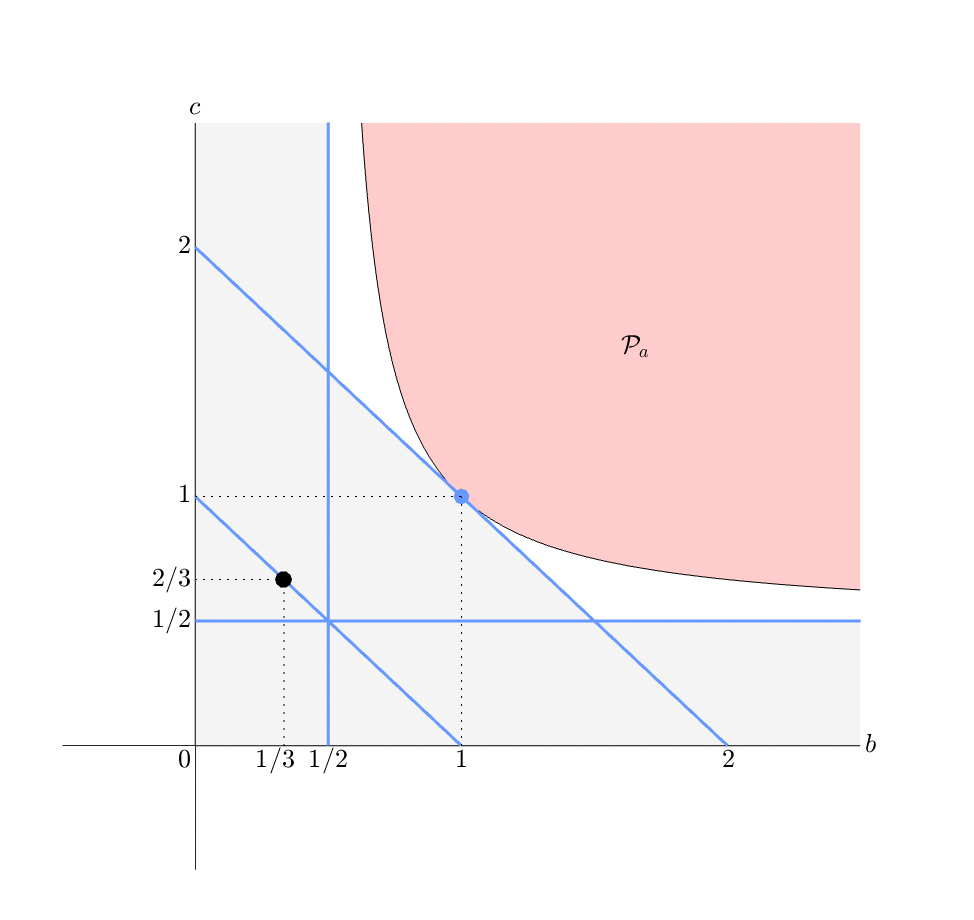
In the special instance the line segment passes through the point for which Craven and Csordas [5] proved that the entire function defined by
belongs to the class and thus this result gives an extension of their work. By combining with the above two types, we illustrate in Figure 7.1 the parameter regions for in the case
3. In the last place, let us consider the case for which defined by (7.1) belongs to . Since if we apply the transference principle, for fixed , then we find that for We now fix and apply the transference principle to the -parameter range as follows:
-
•
Let us assume that so that Since only when we may not extend further in the case If we may shift down by one unit. Since only when this extension of amounts to the union of two intervals
when and the interval when
-
•
In the case we have so that shifting down by one unit is meaningless. If we assume, however, that with being a nonnegative integer, we can extend by applying the transference principle in a reverse way. Indeed, the transference principle implies that when the function
belongs to that is, when
Shifting down units further, we find that the condition
is sufficient for the membership provided
What have been proved may be summarized as follows, where the Gaussian symbol of denotes the largest integer not exceeding .
Theorem 7.2.
For let be the set of all ordered-parameter pairs defined by where
and let If then
In the special case this theorem yields in particular
the well-known result established by Pólya and Hille [12].
To illustrate how all of the above criteria could be combined to specify the range of denominator-parameters, we take and consider
| (7.10) |
For convenience, we shall denote by the set of all pairs for which belongs to the Laguerre-Pólya class (see Figure 7.2).
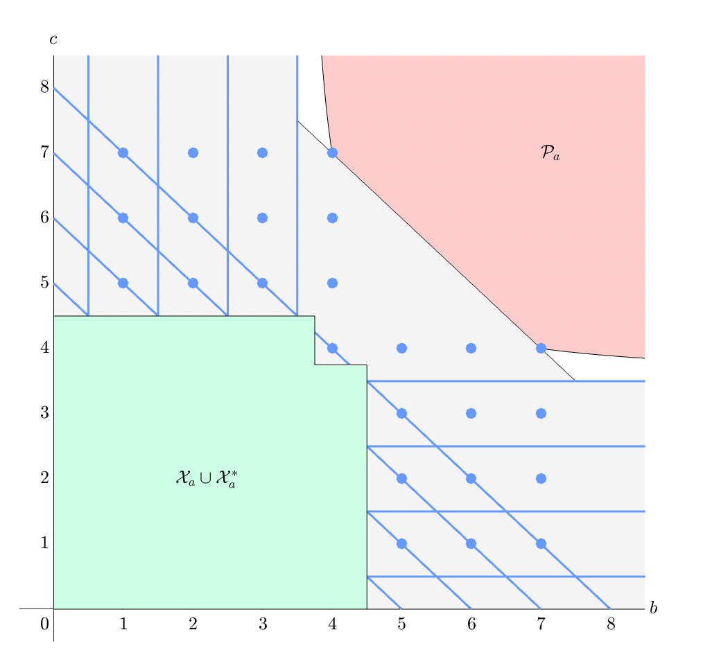
- •
-
•
By inspecting the cases when reduces to Type 1, it is easy to see that contains four vertical rays and four horizontal rays where Similarly, reduces to Type 2 when coincides with one of the lattice points
By symmetry, hence, contains forty such integer-lattice points.
-
•
As is of Type 3, contains eight line segments defined by
-
•
By Theorem 7.2, contains the rectangles
Acknowledgements. Yong-Kum Cho is supported by the National Research Foundation of Korea funded by the Ministry of Science and ICT of Korea (2021R1A2C1007437). Young Woong Park is supported by the Chung-Ang University Graduate Research Scholarship in 2021.
References
- [1] Á. Baricz and S. Koumandos, Turán type inequalities for some Lommel functions of the first kind, Proc. Edinburgh Math. Soc. 59, 569–579 (2016)
- [2] Y.-K. Cho and S.-Y. Chung, Collective interlacing and ranges of the positive zeros of Bessel functions, J. Math. Anal. Appl. 500, 125166 (2021)
- [3] Y.-K. Cho and S.-Y. Chung, The Newton polyhedron and positivity of hypergeometric functions, Constr. Approx. 54, 353–389 (2021)
- [4] Y.-K. Cho, S.-Y. Chung and H. Yun, Rational extension of the Newton diagram for the positivity of hypergeometric functions and Askey-Szegö problem, Constr. Approx. 51, 49–72 (2020)
- [5] T. Craven and G. Csordas, The Fox-Wright functions and Laguerre multiplier sequences, J. Math. Anal. Appl. 314, 109–125 (2006)
- [6] D. K. Dimitrov and P. K. Rusev, Zeros of entire Fourier transforms, East J. Approx. 17, 1–108 (2011)
- [7] A. Erdélyi, W. Magnus, F. Oberhettinger and F. G. Tricomi, Tables of Integral Transforms, Vol. II, McGraw-Hill (1954)
- [8] G. Gasper, Positive integrals of Bessel functions, SIAM J. Math. Anal. 6, 868–881 (1975)
- [9] G. P. Gupta and M. E. Muldoon, Riccati equations and convolution formulae for functions of Rayleigh type, J. Phys. A 33, 1363–1368 (2000)
- [10] J. R. Higgins, An interpolation series associated with the Bessel-Hankel transform, J. London Math. Soc. 5, 707–714 (1972)
- [11] J. R. Higgins, Five short stories about the cardinal series, Bull. Amer. Math. Soc. 12, 45–88 (1985)
- [12] E. Hille, Note on some hypergeometric series of higher order, J. London Math. Soc. 4, 50–54 (1929)
- [13] M. E. H. Ismail and M. E. Muldoon, On the variation with respect to a parameter of zeros of Bessel and q-Bessel functions, J. Math. Anal. Appl. 135, 187–207 (1988)
- [14] A. J. Jerri, The Shannon sampling theorem-Its various extensions and applications: A tutorial review, Proc. IEEE 65, 1565–1595 (1977)
- [15] A. Laforgia and M. Muldoon, Some consequences of the Sturm comparison theorem, Amer. Math. Monthly 93, 89–94 (1986)
- [16] B. Ya. Levin, Lectures on Entire Functions, Translations of Mathematical Monographs 150, Amer. Math. Soc. (1996)
- [17] Y. L. Luke, The Special Functions and Their Approxiations, Vol. I., Academic Press, New York (1969)
- [18] E. Makai, On a monotonic property of certain Sturm-Liouville functions, Acta Math. Acad. Sci. Hungar. 3, 165–172 (1952)
- [19] E. Makai, On zeros of Bessel functions, Univ. Beograd Publ. Elektrotehn. Fak. Ser. Mat. Fiz., no. 602-633, 109–110 (1978)
- [20] G. Pólya, Über die Nullstellen gewisser ganzer Funktionen, Math. Z. 2, 352–383 (1918)
- [21] I. N. Sneddon, On some infinite series involving the zeros of Bessel functions of the first kind, Proc. Glasgow Math. Assoc. 4, 144–156 (1960)
- [22] A. D. Sokal, When does a hypergeometric function belong to the Laguerre-Pólya class ?, J. Math. Anal. Appl., 126432 (2022)
- [23] C. Sturm, Mémoire sur les équations différentielles du second order, J. Math. Pures Appl. 1, 106–186 (1836)
- [24] G. N. Watson, A Treatise on the Theory of Bessel Functions, Cambridge University Press, London (1922)