Island myriads in periodic potentials

Abstract

A phenomenon of emergence of stability islands in phase-space is reported for two periodic potentials with tiling symmetries, one square and the other hexagonal, inspired by bidimensional Hamiltonian models of optical lattices. The structures found, here termed as island myriads, resemble web-tori with notable fractality and arise at energy levels reaching that of unstable equilibria. In general, the myriad is an arrangement of concentric island chains with properties relying on the translational and rotational symmetries of the potential functions. In the square system, orbits within the myriad come in isochronous pairs and can have different periodic closure, either returning to their initial position or jumping to identical sites in neighbor cells of the lattice, therefore impacting transport properties. As seen when compared to a more generic case, i.e. the rectangular lattice, the breaking of square symmetry disrupts the myriad even for small deviations from its equilateral configuration. For the hexagonal case, the myriad was found but in attenuated form, mostly due to extra instabilities in the potential surface that prevent the stabilization of orbits forming the chains.

A phenomenon of appearance of multi-oscillatory motion, here called island myriads, is reported for periodic potentials inspired by Hamiltonian models of two-dimensional optical lattices. The two types of potentials considered here have a periodic structure with square and hexagonal symmetries, allowing them to tile the plane completely. This periodic tiling aspect, and its connection to translational and rotational symmetries, is shown to be responsible for the existence of stable periodic orbits which will form the complex fractal-like structure that is the myriad. The effect of breaking these symmetries is also analyzed. Besides, despite being related to the appearance of stable trajectories, the phenomenon takes place at energy values close to unstable equilibrium points of the potential surface.

I Introduction

In a broad sense, among the various dynamical behaviors seen in Hamiltonian systems, the bifurcation of periodic orbits provides the main approach for describing changes in phase-space as one alters the control parameters of a model. Particularly within area-preserving systems with more than one degree of freedom, bifurcations are extensively documented in the literature Contopoulos . In this scenario, stable periodic orbits represent the elliptic centers of islands whereas when unstable they represent hyperbolic points, with their manifolds governing the dynamics within chaotic regions. As periodic solutions appear, disappear or change stability, they modify the kinetics of the system, thus being commonly referred to as the skeleton of phase-space dynamics.

These bifurcation processes are then applied in studies of the onset of chaos for resonant islands with commensurate frequency (in the context of KAM theorem Walker-Ford ); in the disruption of transport barriers, whether in twist or non-twist systems Castillo-Negrete ; to the existence of multiple oscillatory solutions (in the context of Birkhoff’s theorem Reichl ); or diffusion Zaslavsky_2 , among others.

A peculiar scenario is the one of web-tori, where a multitude of islands tiles a portion of phase-space, corresponding to a different bifurcation condition than that of KAM islands Zaslavsky . In KAM theory, the persistence of invariant tori for a Hamiltonian $H_{0}(I)$ that is monotonic in the actions $I=(I_{1},...,I_{n})$, is guaranteed for nonlinear perturbations with small enough amplitude. In the case of web-tori, the non-degeneracy condition is not satisfied, therewith allowing for the generation of multiple islands depending on the number of fixed points from the equations of motion and the frequency of the oscillatory perturbation. Despite the good introduction to the topic given by ZaslavskyZaslavsky_2 and Chernikov Chernikov , not many works concern a detailed description of the properties of web-tori. This configuration is mostly studied as a framework for weak chaos within stochastic webs, when separatrices are slightly perturbed forming thin chaotic channels with anomalous transport.

In this work, two Hamiltonian systems with periodic potentials, based on optical lattice models, are used to report a bifurcation phenomenon here named as island myriad. The myriad is a seemingly dense filling of a finite region of phase-space by a series of stability islands, highly resembling finite web-tori with notable fractality. It emerges from the bifurcation of orbits scattered when approaching a set of unstable equilibria with the same energy in potential surfaces with tiling symmetry. At the energy level of these equilibria, the deviated orbits form a fractal arrangement of isochronous island chains in phase-space, with each one being formed by rotated and translated symmetrical sets of orbits as allowed by the potential symmetries. The two lattice models considered here have rectangular and hexagonal bidimensional tilings, and the myriad phenomenon is described in terms of its main periodic orbits and shown to rely on the symmetries of the potential functions.

Although the myriad was already reported in a previous work, the results presented here extend and are connected to the previous study done on the square lattice system Lazarotto , to which we refer the reader for additional aspects of the dynamics regarding diffusion.

In what follows, section II starts with deducing the periodic potentials and further Hamiltonians for the selected systems, as inspired by a classical treatment of an optical lattice model. The island myriad bifurcation is initially presented for the square lattice at section III and its properties listed for this case. Then, the effect of symmetry breaking is demonstrated by considering a non-equilateral tiling, i.e. a generic rectangular lattice (sec. IV). At last, the myriad is further analyzed for the hexagonal system (sec. V). Appendices A to C provide details for discussions made along the results sections.

II Lattice hamiltonian model

Periodic potential models have been used as simple yet rich descriptions in different physical contexts, from cold-matter physics Bloch1 , charged particles in plasmas Kleva or diffusion over crystal surfaces Sholl . The kind of periodic potential considered for this work is based on a classical Hamiltonian description of optical lattices.

In these models, when a neutral atom interacts with an electric field $\vec{E}$ from a monochromatic wave, despite its neutrality, a dipole is induced along the field direction Grimm . The induced dipole thus oscillates with the wave while re-interacting with the field, hence submitting the particle to a potential function that, when averaged over time, results in a pondemorative potential

$$\begin{split}V_{\textrm{latt}}&\approx-\frac{\rho(\omega)}{2}\left|\vec{E}(\vec{r})\right|^{2}.\end{split}$$ (1)

Consequently, this conservative potential produces a force over the particle towards the wave antinode (node) if $\rho>0$ ($\rho<0$), thereby constraining the particle along the wave propagation axis.

From the single wave-particle interaction described, a generic lattice is then built by superposing the electric fields from multiple waves oriented throughout 3D space

$$\vec{E}_{\textrm{latt}}(\vec{r})=\sum_{i=1}^{N}\hat{e}_{n}\;E_{0}^{n}\cos\left(\vec{k}_{n}\cdot\vec{r}+\phi_{n}\right)e^{-\mathrm{i}\omega_{n}t},$$ (2)

with each one given by its polarization direction $\hat{e}_{n}$, amplitude $E_{0}^{n}$, wave vector $\vec{k}_{n}$, phase $\phi_{n}$ and angular frequency $\omega_{n}$. Note that $\hat{e}_{n}\cdot\vec{k}_{n}=0\;\forall n$.

For simplicity, all waves are assumed to have equal amplitude, resulting in the generic lattice potential

$$\begin{split}V_{\textrm{latt}}\left(\vec{r}\right)=&\;U^{\prime}\left(\sum_{n=1}^{N}\cos^{2}\left(\vec{k}_{n}\cdot\vec{r}\right)\right.\\ &\left.+2\sum_{n=1}^{N}\sum_{m>n}^{N}\alpha_{nm}\cos\left(\vec{k}_{n}\cdot\vec{r}\right)\cos\left(\vec{k}_{m}\cdot\vec{r}\right)\right)\end{split}$$ (3)

where $\alpha_{nm}=(\hat{e}_{n}\cdot\hat{e}_{m})\cos(\phi_{n}-\phi_{m})$ are the coupling parameters between waves $n$ and $m$ and $U^{\prime}=-\frac{1}{2}\rho(\omega)E_{0}^{2}$. In such a manner, the dynamics of particles is governed by $V_{\textrm{latt}}\left(\vec{r}\right)$ which generally is tridimensional.

In potential (3), a variety of lattices can be built when combining different wave orientations and number. For 2D lattices, at least two co-planar, linearly independent wave vectors must be selected, producing a potential surface over the plane. To provide a $q$-fold symmetry to the lattice, one can set $q$ equally spaced wave vectors with the same norm

$$\vec{k}_{n}=k\cos\left(n\frac{\pi}{q}\right)\hat{x}+k\sin\left(n\frac{\pi}{q}\right)\hat{y},$$ (4)

for $n=0,...,q-1$, generating polygonal lattice patterns.

Therefore, the Hamiltonian for a single particle in a bidimensional lattice is directly written as

$$\begin{split}H^{\prime}=\frac{1}{2m}\left(p_{x}^{2}+p_{y}^{2}\right)+V(x,y).\end{split}$$ (5)

for any lattice potential $V(x,y)$.

II.1 Rectangular lattice

The main lattice type considered here will be a rectangular one, that is, the one formed by two perpendicular waves within the $x\!-\!y$ plane, where $\vec{k}_{x}=k_{x}\hat{x},\;\vec{k}_{y}=k_{y}\hat{y}$, yielding the periodic potential function

$$\begin{split}V(x,y)=U^{\prime}&\left(\cos^{2}(k_{x}x)+\cos^{2}(k_{y}y)\;+\right.\\ &\left.\;2\alpha\cos(k_{x}x)\cos(k_{y}y)\right),\end{split}$$ (6)

with

$$U^{\prime}=-\frac{1}{2}\rho(\omega)E_{0}^{2}\quad\textrm{and}\quad\alpha=\left(\hat{e}_{x}\cdot\hat{e}_{y}\right)\cos(\phi_{x}-\phi_{y}).$$ (7)

The resulting Hamiltonian (5) is re-scaled to $H=2mH^{\prime}$, so that the energy scale is $U=2mU^{\prime}$. In the classical regime, the magnitude of $U$ has no relevance to the topology of solutions whatsoever, with only its sign being relevant. For this work, we consider the case of $U>0$, in which the myriad could be identified. In case $U<0$, the stability of equilibrium points is reversed and the dynamics is considerably different. Therefore, we set $U=20$ in agreement with Horsley et al. Horsley , although for simplicity it could be set to 1 without loss of generality.

The dynamics of a particle will then take place over the potential surface shown in figure 1, where it can be either trapped around minima regions, for energies below those of saddle points between potential wells, or otherwise wander to neighboring cells above this threshold. One may notice that a unit cell for the lattice can be defined as the box $(x,y)\in[-\frac{\pi}{k_{x}},\frac{\pi}{k_{x}}]\times[-\frac{\pi}{k_{y}},\frac{\pi}{k_{y}}]$, allowing for periodic boundary conditions when simulating trajectories (as used in this work when showing trajectories on the lattice unit cell). Notice that the near-symmetry case is when $k_{x}\approx k_{y}$, as the unit cell becomes square.

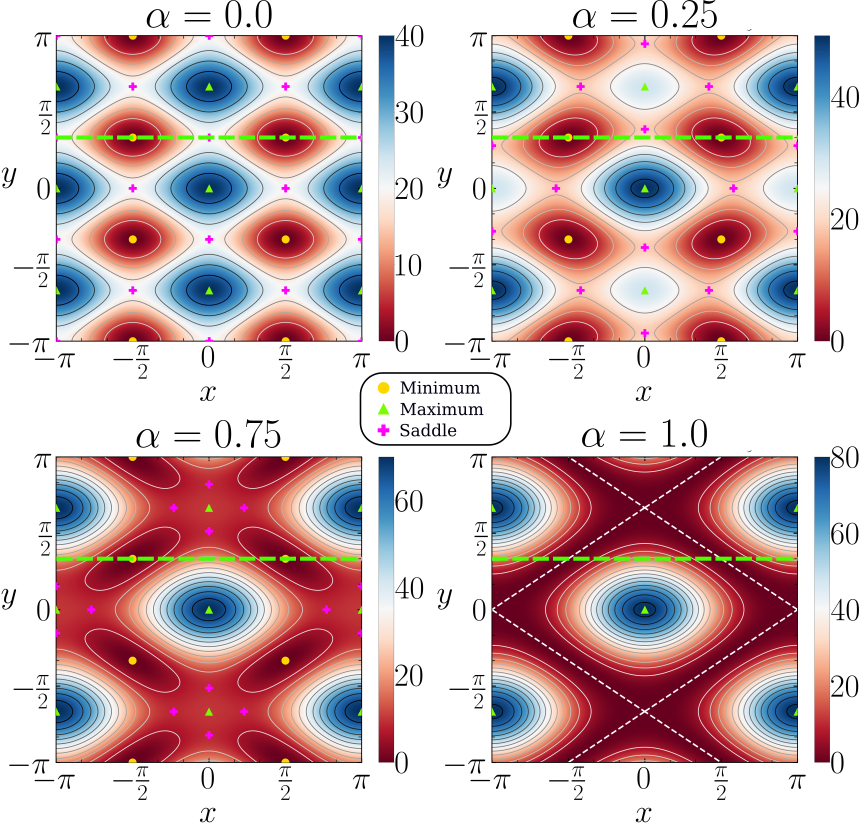
Figure 1: Color plot of the potential surface $V(x,y)$ (eq. 6) for $k_{x}=1,k_{y}=1.5$ and different values of the coupling $\alpha$. The Poincaré section used for phase-space display is shown as the dashed green line at $y=\frac{\pi}{2k_{y}}$. At $\alpha=1$, minima collapse into a ‘minima trench’ given by $\cos(k_{y}y)=-\cos(k_{x}x)$, shown as the white dashed line. Color bars show the value of $V(x,y)$ in normalized units.

For increasing $\alpha$, the potential surface moves from the separable case ($\alpha=0$) to fully superposed ($\alpha=1$) as the equilibrium points change energy and position (see fig. 1 and table 1). While minima remain with zero energy and do not change position with varying $\alpha$, saddle points move towards local maxima, finally merging when $\alpha=1$, forming ‘trench lines’ with degenerate minima along the lines $k_{y}y\pm k_{x}x\equiv\pi\mod(2\pi)$. Simultaneously, local maxima diminish in energy thereby widening the pass between potential wells and facilitating the transport of particles.

As seen in potential (6), the coupling parameter $\alpha$ acts as a perturbation to an integrable Hamiltonian of two uncoupled pendula-like potentials along $x$ and $y$ (with spatial period $\frac{2\pi}{k_{i}}$), coupling them for any $\alpha\neq 0$. Although $\alpha$ may vary in the interval $[-1,1]$, one can limit oneself to solutions for $\alpha\in[0,1]$ as the change $\alpha\to-\alpha$ is equivalent to a spatial translation by $\frac{\pi}{k_{i}}$ in one of the cartesian directions, thus not altering solutions properties.

For the purpose of this work, we start by considering the particular case of a square lattice, that is when $k_{x}=k_{y}$ (which is set as $k=1$ without loss of generality). In general, for any $k_{x}$, $k_{y}$, the rectangular lattice presents translational symmetry for displacements of $\frac{2\pi}{k_{i}}$, for $i=x,y$, along each respective axis. However, the square lattice presents an extra rotation symmetry, by rotations of $\frac{\pi}{2}$. As will be discussed in section III, the presence of symmetry is necessary for the myriad existence. Considering this, we initially analyze the myriad for the square system and then set different $k_{x}$, $k_{y}$ such that symmetry is broken and its effects evaluated. Other alternatives for symmetry breaking are possible, such as the use of non-harmonic waves, as done by Porter et al. Porter1 , although no particular analysis on the bifurcations of orbits is made in that work.

Equilibrium point	$(x^{*},y^{*})$	$V(x^{*},y^{*})$
Minima	$\left(\frac{\pi}{2k_{x}},\frac{\pi}{2k_{y}}\right)$	$0$
	$\left(-\frac{\pi}{2k_{x}},-\frac{\pi}{2k_{y}}\right)$
	$\left(\frac{\pi}{2k_{x}},-\frac{\pi}{2k_{y}}\right)$
	$\left(-\frac{\pi}{2k_{x}},\frac{\pi}{2k_{y}}\right)$
Maxima (global)	$(0,0)$	$2U(1+\alpha)$
	$(\frac{\pi}{k_{x}},\frac{\pi}{k_{y}})$
Maxima (local)	$(\frac{\pi}{k_{x}},0)$	$2U(1-\alpha)$
	$(0,\frac{\pi}{k_{y}})$
Saddles	$(0,\pm\frac{1}{k_{y}}\cos^{-1}(-\alpha))$	$U(1-\alpha^{2})$
	$(\pm\frac{1}{k_{x}}\cos^{-1}(-\alpha),0)$
	$(\frac{\pi}{k_{x}},\pm\frac{1}{k_{y}}\cos^{-1}(\alpha))$
	$(\pm\frac{1}{k_{x}}\cos^{-1}(\alpha),\frac{\pi}{k_{y}})$

Table 1: Equilibrium points position $(x^{*},y^{*})$ and energy $V(x^{*},y^{*})$ within a unit cell of the rectangular lattice potential; positions are taken modulo $2\pi/k_{i}$.

To display phase-space portraits, along all this work the Poincaré section with the oriented surface over two of the lattice minima

$$\Sigma=\left\{\left(x,y,p_{x},p_{y}\right)\in\mathbb{R}^{4};\;y=\frac{\pi}{2k_{y}};\;p_{y}>0\right\}$$ (8)

will be used – as highlighted in green in figure 1. Since Hamiltonian (5) is autonomous, energy ($E=H$) is an immediate constant of motion, constraining trajectories in a three-dimensional surface, which can thus be pictured in a 2D section. For the square lattice, the oriented surface $\Sigma$ is particularly convenient since its projection at the $(x,y)$ plane contains the minima at $x=\pm\frac{\pi}{2k_{x}}$. Indeed, bounded solutions around minima with $y<0$ will occur, but nonetheless the $\frac{\pi}{2}$ rotation invariance implies that their symmetrical rotated counterpart solution will intersect $\Sigma$ at $y=\frac{\pi}{2}$.

II.2 Hexagonal lattice

Analogous to rectangular lattices, hexagonal ones (or honeycomb lattices) are achieved with 3 co-planar wave vectors with same norm and equally spaced by $60^{\textrm{o}}$ from each other, in accordance to equation (4). From equation (3) the resulting potential is given by

$$\begin{split}V(x,y)=U^{\prime}\Bigg{(}&\cos^{2}(kx)+\cos^{2}\left(\frac{k}{2}x+\frac{\sqrt{3}k}{2}y\right)+\cos^{2}\left(-\frac{k}{2}x+\frac{\sqrt{3}k}{2}y\right)+2\alpha_{12}\cos\left(kx\right)\cos\left(\frac{k}{2}x+\frac{\sqrt{3}k}{2}y\right)\\ &+2\alpha_{13}\cos\left(kx\right)\cos\left(-\frac{k}{2}x+\frac{\sqrt{3}k}{2}y\right)+2\alpha_{23}\cos\left(\frac{k}{2}x+\frac{\sqrt{3}k}{2}y\right)\cos\left(-\frac{k}{2}x+\frac{\sqrt{3}k}{2}y\right)\Bigg{)}.\end{split}$$ (9)

The potential form (9) has three coupling parameters $\alpha_{nm}$, implying a 4-dimensional parameter space: ($E,\alpha_{12},\alpha_{13},\alpha_{23}$); it is then convenient to reduce it. For this purpose, figure 2 shows potential surfaces for different values of $\alpha$, notably for cases where all coefficients are equal ($\alpha_{12}=\alpha_{13}=\alpha_{23}=\alpha$). With this condition, some equilibria alter their energy value and stability while remaining in a regular hexagonal structure (fig. 3). Hence, as $\alpha$ varies, the potential surface changes in a similar fashion to that seen for the square lattice, where points may change their energy or stability, while keeping their symmetrical positions with fixed distances (fig. 3, right frame). Although restrictive, this simplification ensures the parameter space reduction and the preservation of symmetry required for the purposes of this study, as will be made clear when discussing the dependence of the myriad phenomenon with the latter aspect.

Figure 2: Color plot of the hexagonal lattice potential (9) for different $\alpha$ values, within the single parameter condition ($\alpha_{nm}=\alpha$). For these figures $U=1$. Color bars show the value of $V(x,y)$ in normalized units.

Nonetheless, since the orientation of one wave-vector alters its coupling with all the other waves, it can be shown that when all $\alpha_{nm}$ are equal, they must lie in the range $\alpha\in[-\frac{1}{2},1]$ (for details, see appendix A).

In this single coupling scenario, the potential can be re-written as

$$V(x,y) = U\Biggl{(}1+\left(\alpha+\cos(x)\right)\cos\left(\sqrt{3}y\right)\Biggr{.}$$ (10)

$$\quad+\cos(x)\Bigl{(}4\alpha\cos\left(\frac{x}{2}\right)\cos\Bigl{(}\frac{\sqrt{3}y}{2}\Bigr{)}\Bigr{.}$$

$$\qquad\qquad\qquad\Biggl{.}\Bigl{.}+\alpha+\cos(x)\Bigr{)}\Biggr{)},$$

and consequently the Hamiltonian is as in equation (5) with $V(x,y)$ either as in equation (9) or (10) and $H$ normalized as in the rectangular lattice. Similar to the rectangular system, for the hexagonal lattice, phase-space displays will be made over the section placed at $y=0$ and oriented as $p_{y}>0$ (dashed black line in the left frame of fig. 3).

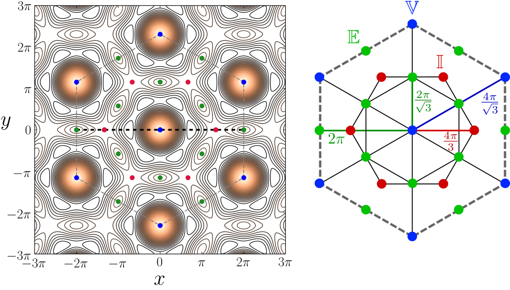
Figure 3: Geometric schematic used for equilibrium points calculation in the hexagonal lattice potential, assuming the single coupling condition. (Left) Equipotential lines (for $\alpha=0.5$) and the selected equilibria. The black dashed line marks the Poincaré section position at $y=0$. (Right) Schematization of the unit cell with the main hexagons and distances used for calculations. Equal colors indicate equal energy levels.

Eq. point	$(x^{*},y^{*})$	$V(x^{*},y^{*})$
$\mathbb{V}$	$(0,\;0)$	$3\left(1+2\alpha\right)$
	$\frac{4\pi}{\sqrt{3}}\left(\cos\left(\frac{(2n+1)\pi}{6}\right),\;\sin\left(\frac{(2n+1)\pi}{6}\right)\right)$
$\mathbb{E}$	$\frac{2\pi}{\sqrt{3}}\left(\cos\left(\frac{(2n+1)\pi}{6}\right),\;\sin\left(\frac{(2n+1)\pi}{6}\right)\right)$	$3-2\alpha$
	$2\pi\left(\cos\left(\frac{n\pi}{3}\right),\;\sin\left(\frac{n\pi}{3}\right)\right)$
$\mathbb{I}$	$\frac{4\pi}{3}\left(\cos\left(\frac{n\pi}{3}\right),\;\sin\left(\frac{n\pi}{3}\right)\right)$	$\frac{3}{4}+\frac{3\alpha}{2}$

Table 2: Equilibrium points position $(x^{*},y^{*})$ and energy $V(x^{*},y^{*})$ for some reference points in the hexagonal unit cell (fig. 3). In the indices above, $n=0,1,2,3,4,5$, modulo $6$. Information on the labels is given in the text.

In the right frame of figure 3, selected equilibria are highlighted over the hexagonal lattice unit cell. They were selected both as geometrical and energetical references related to the expectation to find the island myriad phenomenon. The unit cell vertices and center point are labeled as $\mathbb{V}$; the cell outermost edges and the inner hexagon edges are labeled as $\mathbb{E}$ and the innermost hexagon vertices as $\mathbb{I}$ (see table 2).

III The island myriad – square lattice

We start by presenting the island myriad phenomenon for the square lattice in the context of emergence of stability structures in phase-space. When measuring the area (or volume) of phase-space occupied by islands or chaotic regions as a function of the control parameters $(E,\alpha)$, a series of fluctuations are expected given the mixed nature of nonlinear dynamics. For this purpose, the chaotic/regular areas were measured over the section $\Sigma$ (eq. 8) via a smaller alignment index (SALI) method, as developed by SkokosSkokos_paper ; Skokos_book .

Briefly, the algorithm integrates a single orbit along with two deviation vectors ($\vec{\omega}_{1}(t),\vec{\omega}_{2}(t)$). These vectors are evolved in time by the linearized equations of motion (and rescaled when necessary) and present different behavior depending on the nature of the orbit. In case it is chaotic, the deviation vectors align or anti-align to each other due to the exponential stretching of phase-space along the unstable manifold direction. On the other hand, if the orbit is regular, ($\vec{\omega}_{1},\vec{\omega}_{2}$) are kept at finite angle (up to secular drift) while only orienting themselves towards the tangent plane of the stable torus in which the orbit is contained. Therefore, the evaluation of this alignment, achieved by the index function

$$\textrm{SALI}(t)\coloneqq\textrm{min}\left(\lVert\hat{\omega}_{1}(t)+\hat{\omega}_{2}(t)\rVert,\lVert\hat{\omega}_{1}(t)-\hat{\omega}_{2}(t)\rVert\right),$$ (11)

can numerically discriminate the orbit’s stability, such that SALI($t$) $\to 0$ exponentially as $t\to\infty$ for chaotic orbits, while it keeps an essentially constant non-zero value for regular ones (SALI$(t)\in(0,\sqrt{2}]$ – for normalized $\hat{\omega}_{i}=\vec{\omega}_{i}/|\vec{\omega}_{i}|$)). It is possible that for regular orbits the tangent vectors still align/anti-align due to shear between close torus layers; however, this was seen to occur over times much longer than the one for alignment in chaotic orbits.

Using such a discrimination index, the chaotic/regular areas are then identified over a 2D fine mesh of the surface $\Sigma$, where each area tile is attributed to an initial condition and all tiles are summed at the end. Figure 4 shows a color map of the chaotic area percentage ($A$) of phase-space along all parameter space ($E,\alpha$), revealing a series of patterns of emergence and disappearance of stability structures (white regions – $A\approx 0.0$). As seen in the bottom frame, two particular lines stand out with the dominance of stability structures as well as borders to the global chaos limit of the system ($A\approx 1.0$). These straight pixelated lines with $A\approx 0$ are seen to coincide with the energy levels $E(\alpha)$ of maxima of the square lattice potential, being negatively (positively) inclined for local (global) maxima (eq. 6 and table 1), as highlighted in the lower frame.

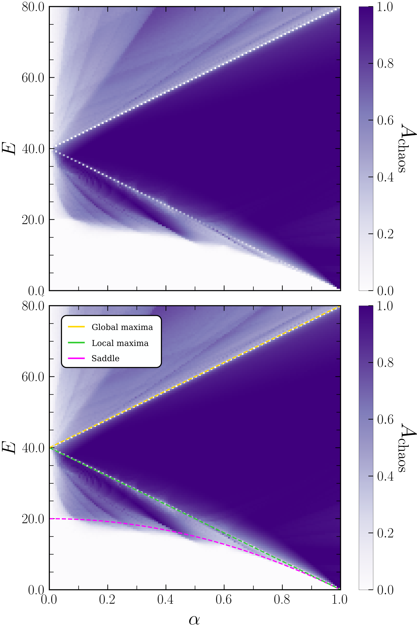
Figure 4: Color map of the chaotic area portion in parameter space for the square lattice. Total chaos is indicated by $A=1$ and total regularity by $A=0$. In the top frame, the seemingly dotted white lines are an artifact of grid pixel precision. In the bottom frame, energy lines for equilibrium points are displayed as: $V_{\textrm{saddle}}=U(1-\alpha^{2})$ in magenta; $V_{\textrm{l-max}}=2U(1-\alpha)$ in green and $V_{\textrm{g-max}}=2U(1+\alpha)$ in yellow. Grid size is $250\times 250$.

In the light of this, it is seen that when the system energy reaches that of unstable equilibria, either local or global, stability structures emerge in phase-space. These structures are a myriad of island chains, as illustrated in figure 5 for the case of $\alpha=0.1$ and $E=36$ (over the local maxima energy line – in green in figure 4). Below local maxima energy, phase-space is dominated by a chaotic sea with three main stability islands. As energy approaches the local maximum level, the two bottommost islands vanish and the chaotic sea is filled with a multitude of island chains. Right above the local-maxima level ($E\approx 36.6$), the myriad completely vanishes and phase-space is again dominated by a uniform chaotic sea.

The observed chains have always even period and are all concentric around the hyperbolic fixed point located at $(x,\frac{p_{x}}{\sqrt{E}})\approx(\frac{\pi}{2},-0.71$), forming an onion-like structure with apparent fractality, as higher period chains appear in between smaller period ones (fig. 6). The mentioned hyperbolic point corresponds to the unstable periodic orbit located along the local maxima at $(x_{\textrm{loc}},y_{\textrm{loc}})=(0,\pi)$ and $(x_{\textrm{loc}},y_{\textrm{loc}})=(\pi,0)$. The myriad is more clearly visible in parameter space for $\alpha\lesssim 0.6$ and inside a short energy window of $\Delta E\approx 0.5$ above maxima energy values.

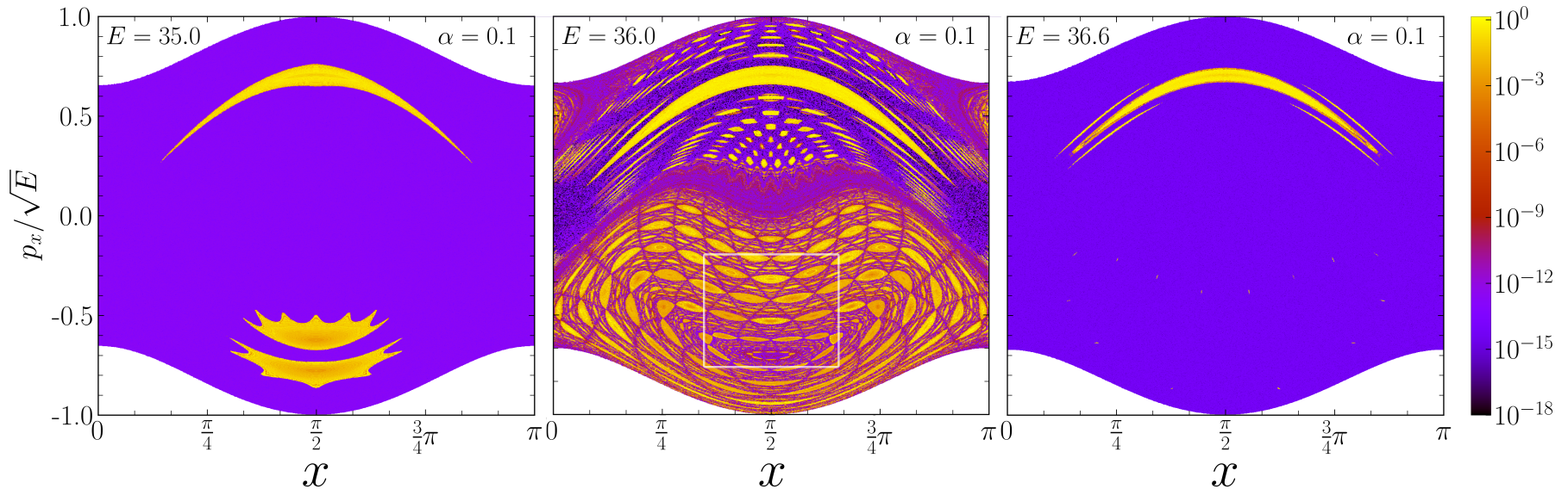
Figure 5: Colorized section $\Sigma$ for varying energy $E$. (Left) $E=35$, below local maxima energy. (Center) Island myriad at $E=36$, exactly at local maxima level: $V_{\textrm{local}}(\alpha=0.1)$ (table 1) – the white square indicates a zoom in shown in figure 6. (Right) $E=36.6$, after the myriad disappearance. Colors were set using the SALI$(t)$ index value to emphasize islands (in yellow) from chaos (in purple).

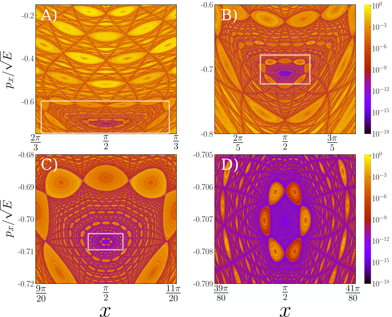
Figure 6: Colorized phase-space of the island myriad for $\alpha=0.1$ and $E=36$ showing successive zooms into the myriad core. A) zoom in from the central frame of figure 5. B) zoom in from frame A. C) zoom in from frame B. D) zoom in from frame C.

As mentioned earlier, a similar stability emergence is seen around global maxima energy lines (yellow line in figure 4). The myriad structure for this scenario is qualitatively similar to the one seen over local maxima lines, as shown in appendix B, so it will not be detailed in this work, which mainly focuses on case of local maxima energy levels.

III.1 Isochronicity

An individual island chain is not related to a single stable periodic orbit and its set of elliptic fixed points, as one usually expects. Instead, all chains in the myriad are isochronous, in the sense that they are formed by two (or more) independent sets of interleaved island links, where orbits contained in one set do not overlap with the other, as illustrated in figure 7.

The isochronous condition can be found in many dynamical systems Sousa ; Bruno but here its origin is clearly seen as a consequence of the system symmetries. As an example, figure 7 shows that the orbits forming each chain set are symmetric pairs (blue and red orbits for the period 8 chain, and yellow and black orbits for the period 10), i.e. they are rotated by $(l+1)\frac{\pi}{2}$ or translated by ($n\pi,m\pi)$ in space, for $l,m,n\in\mathbb{Z}$, relative to each other. Since they are the same geometrical curve, they present the same period and rotation number, therefore emerging in the same torus layer. Indeed, this is an immediate consequence of the square lattice potential translational and rotational symmetries, as well as its ‘tiling’ closure property, the same allowing for the use of periodic boundary conditions. In general, chains in the myriad present double isochronicity, being split into two orbit sets; however, triple isochronicity can also be found, as better detailed in appendix C.

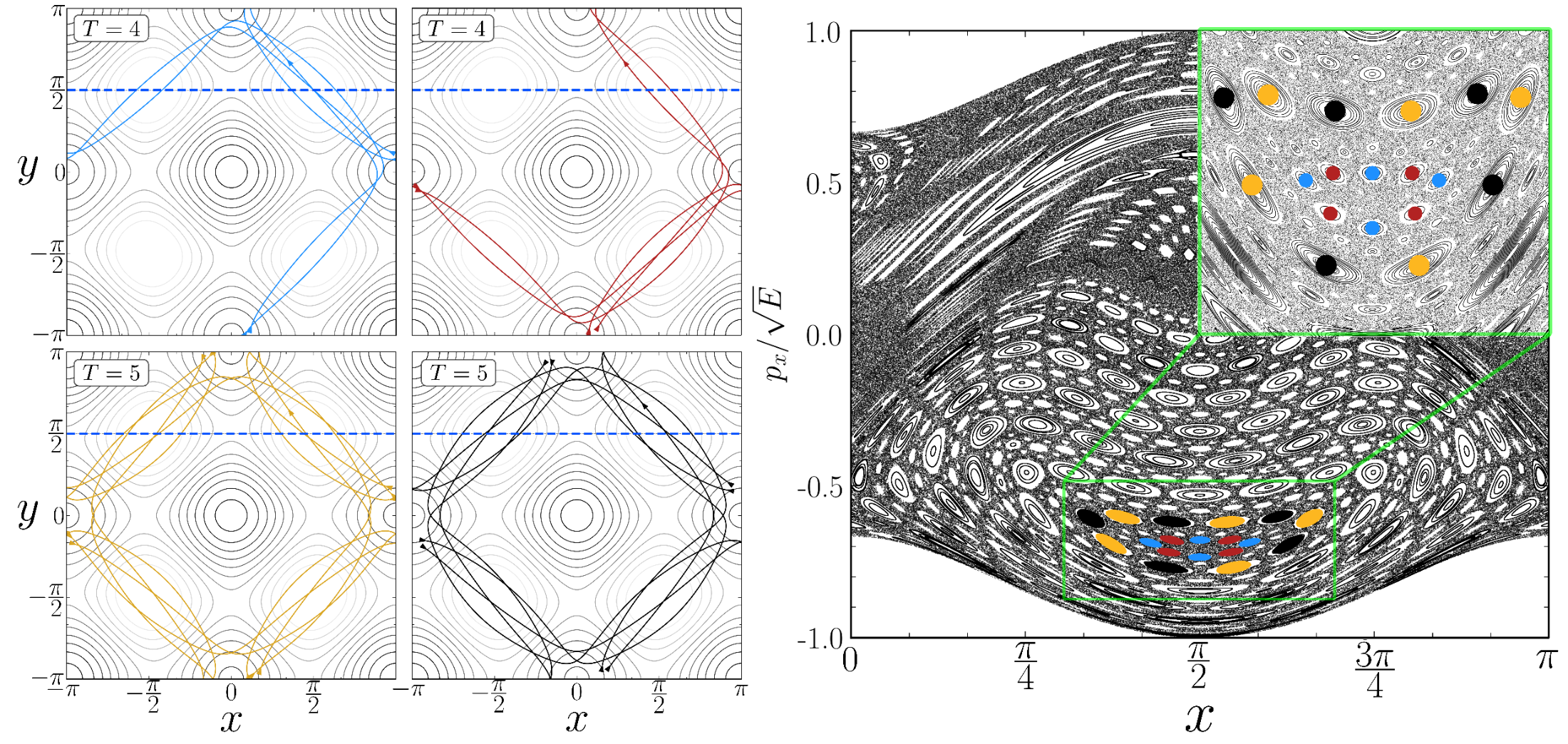
Figure 7: (Left) Isochronous periodic orbits from two island myriad chains, shown in the square lattice unit cell. (Right) Poincaré section with the myriad structure. Colored dots indicate the elliptic fixed points of the orbits relative to the section $\Sigma$ (blue dotted line); $T$ indicates the fixed point period. The innermost period 8 chain is formed by the blue and red sets, while the immediate next one, with period 10, by the yellow and black ones.

III.2 Escape time (periodic spatial closure)

When inspecting the stable periodic orbits associated with different chain layers in the myriad, distinct periodic behaviors are seen. In one case, orbits return to their exact initial position even when disregarding periodic boundary conditions (as in a libration), whereas in the other they only do so with them (as in a rotation), as exemplified in figure 8. This difference in spatial closure therefore directly impacts the transport properties between different myriad layers. In this context, escape time basins are simply defined as a color map of the time required for initial conditions on the section $\Sigma$ (within a central unit cell) to reach outside the square box with $n$ unit cells of size, i.e., $x,y\in\left[-n\pi,n\pi\right]$ (here $n=20$).

As seen among the interleaved chains, in yellow escape time basins in figure 9, orbits from islands with librational movement (top frames in fig. 8) remain trapped while the ones from purple basins with rotational movement (bottom frames in fig. 8) quickly escape in direct flights through the lattice. This is only possible due to the periodic ‘tiling’ property of the potential function, as translated positions $(x,y)\to(x\pm 2n\pi,y\pm 2m\pi)$, for $n,m\in\mathbb{Z}$, will correspond to an identical site in a neighbor unit cell, thus allowing for periodic behavior without return to the exact initial position.

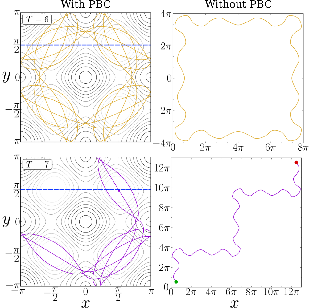
Figure 8: Examples of periodic orbits with different spatial closures. On the left column, trajectories within the unit cell and boundary conditions applied. On the right column, the same trajectories without boundary conditions, ranging through all space.

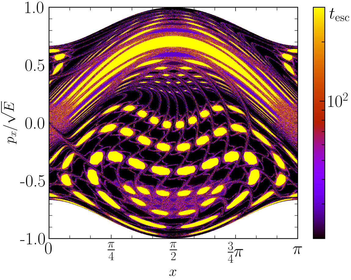
Figure 9: Color map of escape time ($t_{\textrm{esc}}$) basins over the island myriad. System parameters are $\alpha=0.1$, $E=36.05$.

III.3 Separatrix reconnection

As asserted initially, the island myriad is expected to emerge when orbits reach the energy level of unstable equilibria of the lattice. However, the energy of these points themselves changes with the coupling $\alpha$, thereby raising the possibility of analysing the myriad evolution as the unstable points change.

Qualitatively, it was found that when varying the energy over the local maxima line for increasing coupling, i.e. $E=V_{\textrm{l-max}}=2U(1-\alpha)$ (in green in fig. 4), all island chains move outwards from the myriad center; simultaneously, islands external to the myriad core, from an external layer surrounding the myriad, move inwards, eventually ‘colliding’ with the outgoing inner island chains.

The ‘collision’ (or superposition) of these island chains gives rise to a bifurcation process eventually leading to the disappearance of both chains. Particularly, this bifurcation process occurs via a separatrix reconnection, as illustrated for a pair of chains of period 4, in figure 10, and a pair of period 6, in figure 11. In this process, the outer and inner chains are interdigitated relative to each other, in the sense that the stable centers of islands from one chain align with the saddles (unstable points) of the other. When colliding, the separatrix is divided while changing its configuration, with the previous outermost chain now inside the center myriad structure and the former inner chain immersed in the chaotic area. This process keeps on going continuously and sequentially as the inner chains move outwards, always in an interdigitated configuration relative to the outer ones, then reconnecting and further disappearing, eroding the myriad with chaos until it vanishes for $\alpha=1$ and $E=0$.

Figure 10: Separatrix reconnection of islands of period 4 within the myriad as ($\alpha$, $E$) vary on the local maxima line in the square lattice. The coupling increases from top to bottom, $\alpha=0.295\to 0.305$ and $E=V_{\textrm{l-max}}(\alpha)$.

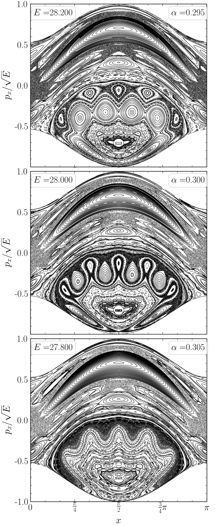
Figure 11: Separatrix reconnection of islands of period 6 within the myriad as ($\alpha$, $E$) vary on the local maxima line in the square lattice. The coupling increases from top to bottom, $\alpha=0.395\to 0.415$ and $E=V_{\textrm{l-max}}(\alpha)$.

Commonly, the scenario of separatrix reconnection is seen in non-twist systems, widely studied in their standard form Castillo-Negrete ; Morrison . In such systems, the twist property, i.e. the monotonic increase of the winding number with the action variable, is violated, presenting points of maximum or minimum. In case resonances appear around these extreme points, they form an interdigitated island chain pair, similar to that seen in figures 10 and 11. At the same time, the curve between them, exactly at the extreme point, is a shearless curve which acts as a transport barrier between chaotic regions in phase-space. Here, a similar arrangement is seen when considering the local winding number relative to the island myriad center. The supposed shearless curve would thus be expected to occur between the interdigitated islands that reconnect; however, higher order bifurcations and the constant presence of a chaotic layer between them prevents a direct verification via winding number profile and can indicate that the curve is destroyed.

IV Island myriad – rectangular lattice

The results obtained for the square lattice highlight the dependence of the myriad phenomenon on the tiling symmetry of the potential function, which stands from the assumption $k_{x}=k_{y}$. For this purpose, this section verifies to what extent the breaking of this symmetry affects the phenomenon.

When setting $k_{x}\neq k_{y}$, the rotation symmetry is lost, although translation symmetry is still preserved for translations by $\frac{2\pi}{k_{i}}$, for $i=x,y$, along the axis. Nevertheless, the stable periodic orbits that form the myriad observed in the square system may be deformed or change their stability as symmetry is broken, preventing its emergence.

A verification of the myriad disappearance was carried out by measuring of the regular area profile for a fixed coupling value and varying energy, as the value of $k_{y}$ changes from the square case ($k_{x}=k_{y}=1$) to asymmetric scenarios. Figure 12 shows that, as the energy reaches the local maxima ($E=V_{\textrm{local}}=36$, for $\alpha=0.1$), the regular area presents a sudden peak, as expected for the square case $k_{y}=1$. As asymmetry grows with increasing $k_{y}$, this peak is quickly suppressed, with the myriad completely vanishing when $k_{y}\simeq 1.100$. This effect is also verified in phase-space portraits A to C in figure 13, with the myriad being eroded by chaos. The same trend is seen for the myriad relative to the global maxima energy level ($E=V_{\textrm{global}}=44$, for $\alpha=0.1$).

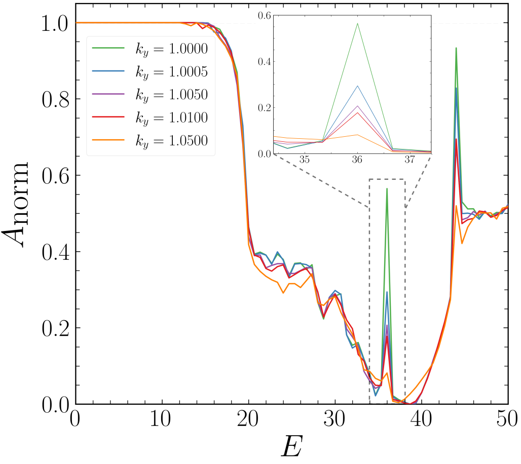
Figure 12: Regular area (normalized to total area $A_{\textrm{total}}=A_{\textrm{regular}}+A_{\textrm{chaos}}=1$) as a function of energy and fixed coupling ($\alpha=0.1$) for increasing $k_{y}$ as asymmetry grows in the rectangular lattice.

Furthermore, for even larger $k_{y}$ ($k_{y}>1.2$), a stabilization is seen in phase-space for larger values of momentum, as shown in portraits D to F. Primarily for the bottommost region of the Poincaré section, for $p_{x}\approx-\sqrt{E}$, and later for the uppermost region $p_{x}\approx+\sqrt{E}$, islands and invariant curves appear and grow in area as the asymmetry between the $x$ and $y$ axes becomes more pronounced. This indicates that the creation of a movement channel along the $y$ axis with a period different from the one along $x$ induces the stabilization of long flights, implying a pendulum-like dynamics along $x$ in the limit that its movement becomes uncoupled from the one in $y$.

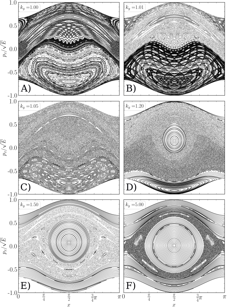
Figure 13: Poincaré section portraits of the island myriad for fixed energy ($E=36$) and coupling ($\alpha=0.1$) and increasing $k_{y}$. A) $k_{y}=1$ (square case); B) $k_{y}=1.01$; C) $k_{y}=1.05$; D) $k_{y}=1.2$; E) $k_{y}=1.5$; F) $k_{y}=5$.

V Island myriad – hexagonal lattice

From the premise that the myriad relies on the potential function symmetries, we extend the investigation to a hexagonal system, as the next polygon with tiling property. Therewith, as done for the regular square system, the chaotic and regular area portions are shown in figure 14.

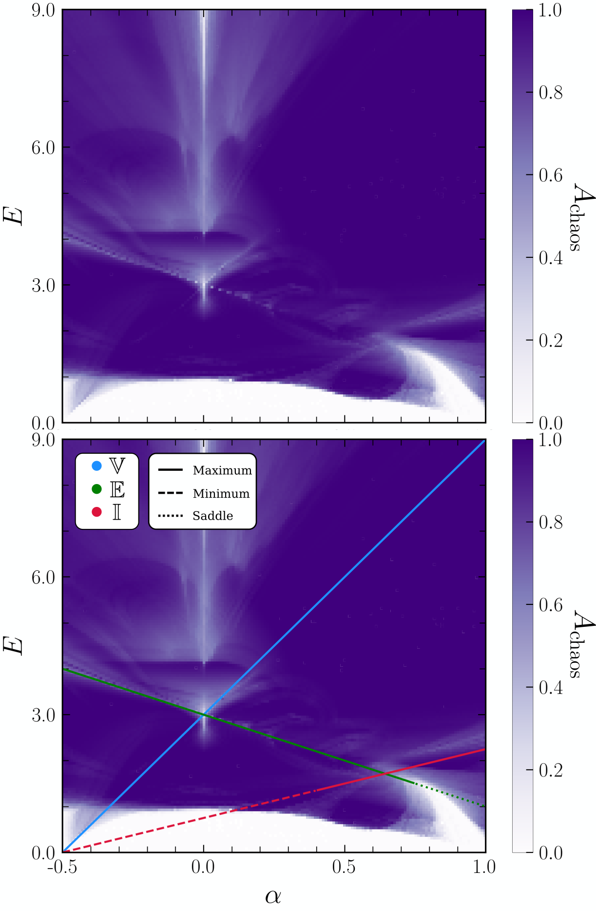
Figure 14: Color map of the chaotic area portion in parameter space for the hexagonal lattice. Total chaos (regularity) is indicated by $A=1$ ($A=0$). In the bottom frame, energy lines colors correspond to the equilibria displayed following table 2 and the texture of the line stands for the point stability. Grid size is $250\times 250$.

As conjectured, the myriad is expected to emerge at energy levels of maxima of the potential surface. However, in the hexagonal system, this correlation is not so prominent as in the square case. Indeed, the only region where it is clearly identified is near $\alpha\approx 0$, over the $V(\mathbb{E},\alpha)=3-2\alpha$ line (in green in fig. 14). The myriad found is shown in phase-space in figures 15 and 16 for $\alpha\gtrsim 0$ and $\alpha\lesssim 0$, respectively. Despite the general similarity, for $\alpha\gtrsim 0$ the island chains surround only the center island, relative to a bounded periodic orbit (in purple in fig. 15), whereas for $\alpha\lesssim 0$ the island chains surround all 4 major islands.

At $\alpha=0.0$, the parameter space reveals a vertical line with increased stable area seen for $E>2.5$, as expected from a myriad structure. However, this increase was seen to be related to the stabilization of the 4 major islands shown in figures 15 and 16 and satellite islands, although not as a myriad. It becomes apparent then that at null coupling, where both $\mathbb{E}$ and $\mathbb{V}$ points are isoenergetic maxima, the inner triangulations within the unit cell, despite increasing symmetry, are not enough to form a myriad but instead changing $\alpha$ increases the stability area of the 4 main island orbits.

Despite the lack of visible fractality in the myriad as seen in the square system, the chaotic region in between chains present a strong stickiness behavior, acting as a permeable barrier for chaotic transport from the chaotic sea into the myriad core. Indeed, the myriad in the hexagonal system seems to be affected by other instabilities in the potential surface caused by saddle and maxima points not listed here, preventing the existence or stabilization of periodic orbits to form the chains.

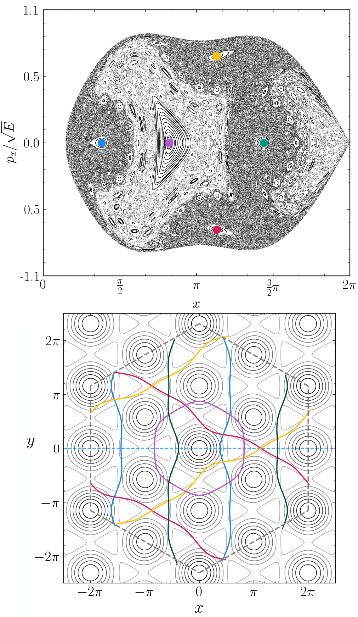
Figure 15: (Top) Island myriad in the hexagonal lattice as seen on the Poincaré section ($y=0;p_{y}>0$) for $\alpha=0.04$ and $E=V(\mathbb{E},\alpha)=2.92$. (Bottom) Stable periodic orbits for the main stability islands shown in the hexagonal unit cell.

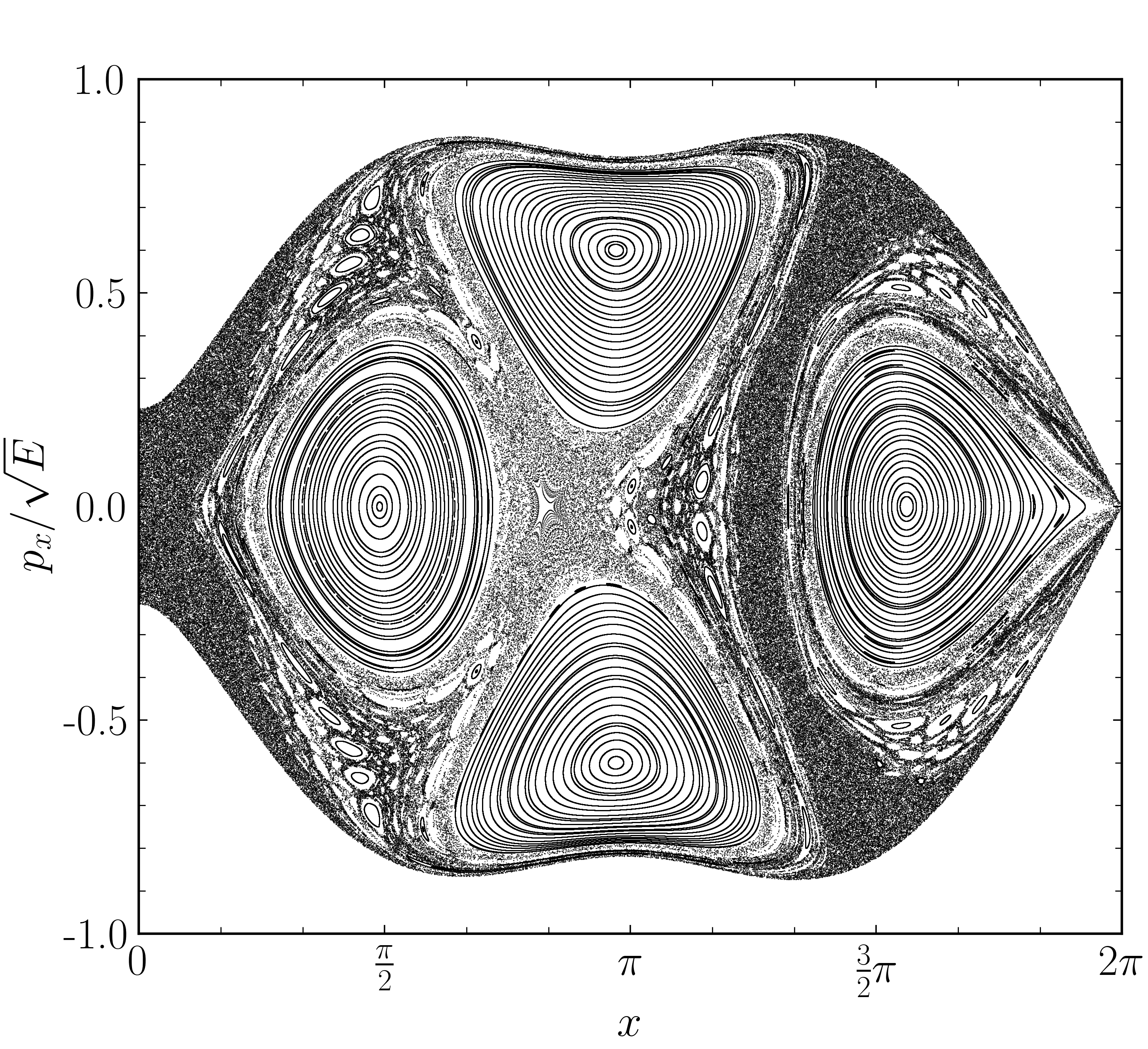
Figure 16: Island myriad in the hexagonal lattice as seen from the Poincaré section ($y=0;p_{y}>0$) for $\alpha=-0.02$ and $E=V(\mathbb{E},\alpha)=3.04$.

Besides the lack of pronounced fractality, the orbits comprising the myriad present less varied features regarding its periodic closure and isochronicity as compared to the ones seen in the square system. For example, figure 17 shows the escape time pattern over the section from figure 15, revealing only trapped orbits (in yellow) through all myriad chains. Also, the stickiness in between chains become clearer once the chaotic region inside the myriad core has trapped orbits (up to time $t=6\times 10^{3}$) despite being connected to the outer chaotic sea.

Regarding isochronicity, once the hexagonal tiling has a three-fold rotation symmetry (from its three symmetry axes, $60^{o}$ apart from each other), the multiplicity of most chains is also three-folded, as exemplified in figures 18 and 19. In this case, the orbits are invariant under rotations of $\pi/3$, thus not altering their fixed point period when rotated. For this reason, isochronous orbits are simple translations from one another. In figure 18, using the yellow orbit as a reference, the red orbit is translated in the $\hat{t}_{y\to r}=(\frac{\sqrt{3}}{2},-\frac{1}{2})$ direction and the blue one along $\hat{t}_{y\to b}=(0,-1)$. Similarly in figure 19, the yellow to red translation is along $\hat{t}_{y\to r}=(\frac{1}{2},\frac{\sqrt{3}}{2})$ and the red to blue along $\hat{t}_{r\to b}=(0,-1)$. As seen for the square system, higher multiplicity chains may occur, but none was found for this case.

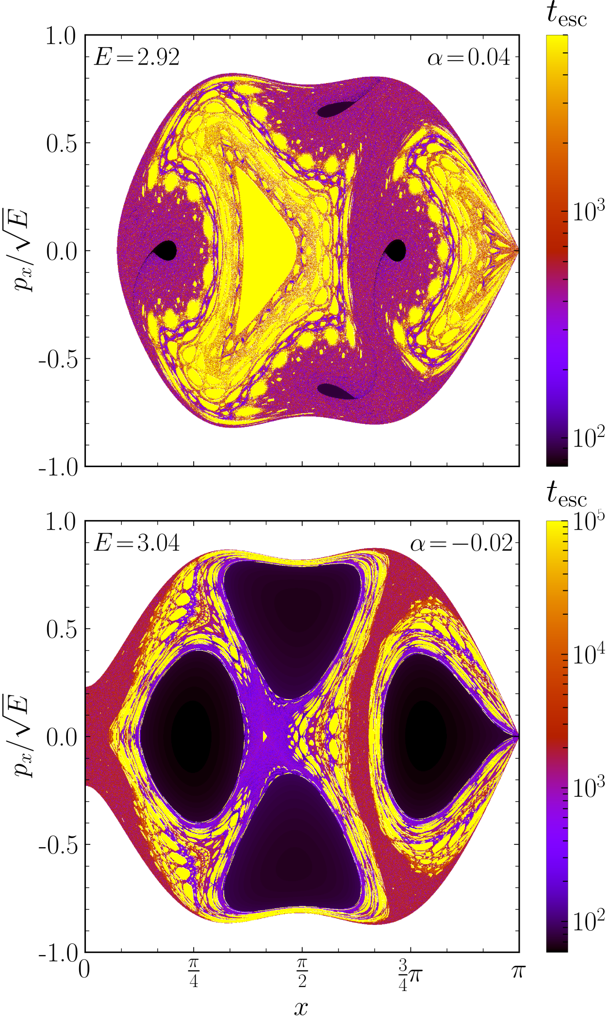
Figure 17: Escape time ($t_{\textrm{esc}}$) color map over the Poincaré section ($y=0;p_{y}>0$) for the hexagonal lattice. (Top) $E=2.92$, $\alpha=0.04$. (Bottom) $E=3.04$, $\alpha=2.92$.

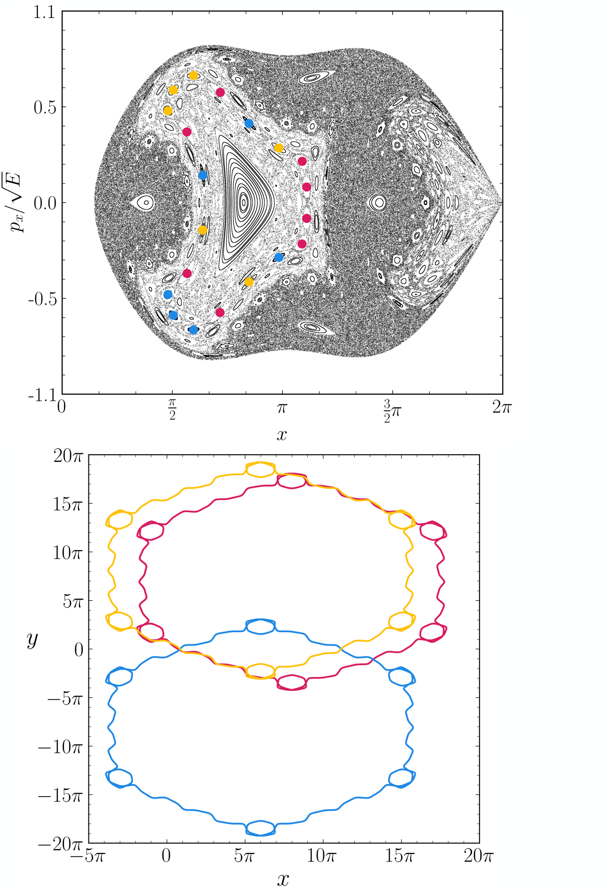
Figure 18: Poincaré section for $E=V(\mathbb{E},\alpha)=2.92$ and $\alpha=0.04$ with selected orbits from a chain with total period $T=20$. (Bottom) Isochronous periodic orbits without periodic boundary conditions: red ($T=8$); blue ($T=6$); yellow ($T=6$).

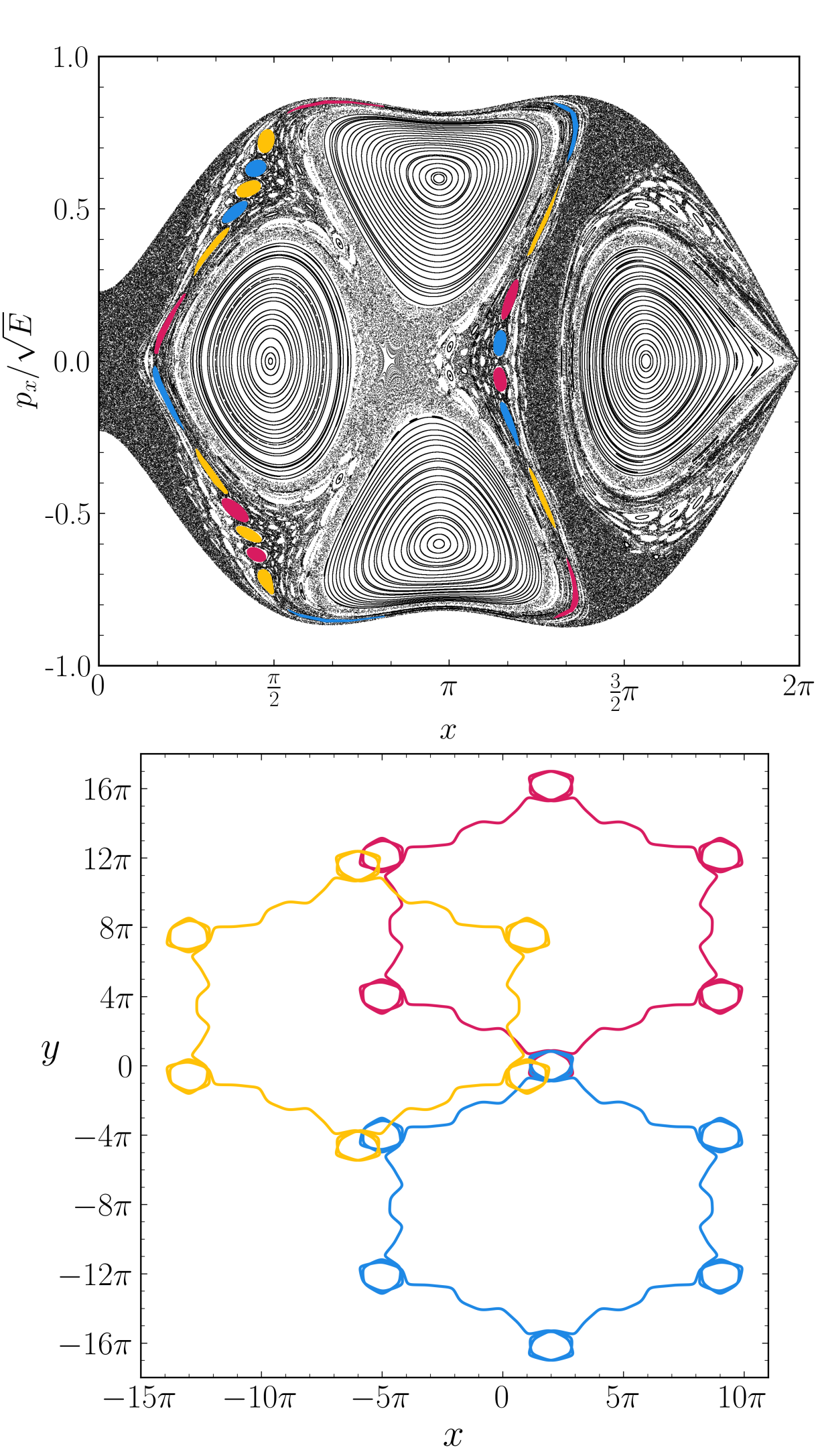
Figure 19: Poincaré section for $E=V(\mathbb{E},\alpha)=3.04$ and $\alpha=-0.02$ with selected orbits from a chain with total period $T=22$. (Bottom) Isochronous periodic orbits without periodic boundary conditions: red ($T=7$); blue ($T=7$); yellow ($T=8$).

VI Conclusions

Fundamentally, the island myriad is seen as the emergence of stability islands at energy levels of maxima in periodic potentials with tiling symmetry. Despite the instability of these equilibrium points, the periodic orbits deviated near these points are stable and appear as concentric layers of island chains in phase-space. A thorough verification over parameter space reveals that this structure is exclusively found over a short energy interval near unstable points, being clearly visible along both local and global maxima for the square lattice, while being restricted to null coupling for the hexagonal case.

The myriad existence relies on the translational, rotational and mirror symmetries of the potential function. This dependence was directly verified when comparing the square lattice with its non-symmetric equivalent form as a rectangular lattice, with asymmetries of 5% being enough to suppress the myriad ($|k_{y}-k_{x}|=0.05$). Moreover, further increasing the asymmetry between the $x$ and $y$ axes for $k_{y}\gg k_{x}$, the dynamics becomes uncoupled and phase-space is stabilized in a pendulum-like configuration, with chaos restricted to separatrix vicinity.

Particularly for the square lattice system, the myriad appears as a finite web-torus with notable fractality, where each chain has an even period split into 2 independent sets of isochronous orbits, although isolated cases with 3 sets were also found. Furthermore, the translational symmetry allows for different periodic closures, in the sense that some periodic orbits return to their initial position whereas others reach identical sites in translated unit cells by $(\Delta x,\Delta y)=(2m\pi,2n\pi)$, for $m,n\in\mathbb{Z}$. The overall effect is the co-existence of trapped orbits (libration – periodically closed) and long flights (rotation – periodically open), therefore affecting global transport. In addition to that, as the coupling parameter was increased, the myriad was seen to undergo separatrix reconnections for each of its layers, destroying them sequentially as they expand outwards the myriad core, suggesting a non-twist local dynamics over the Poincaré section.

One can add to these results our previous findings for the square system regarding the diffusive transport of particles Lazarotto . For the energy level of local maxima, the myriad emergence and sudden disappearance correlates to suppression in global diffusion, with long flights vanishing from the system dynamics. Also, periodic orbits approaching the maxima present a divergence in their period, as in the paradigmatic classic pendulum in its threshold between rotation and libration, therefore promoting a slowing down of the dynamics.

Despite being also confirmed in the hexagonal lattice, as expected from its similar tiling symmetries, the myriad was found in attenuated form. In this case, fractality is less pronounced due to extra saddle and maxima points in the potential surface acting as instability sources, thereby preventing the stabilization of orbits that would form the chains. Also, only periodically closed orbits are found, thus with no simultaneous opposite transport regimes as in the square case.

Although isochronicity, separatrix reconnection and web-tori are already well-documented features of dynamical systems, lattice models present all of them simultaneously in a single structure. Moreover, the simplicity of the model allows for an intuitive understanding of these phenomena in phase-space and their correspondent dynamical behavior in position space. As seen from the periodic orbits that comprise the myriad chains, they are a direct consequence of the potential function symmetries, as opposed to more abstract models.

However, it is not yet intuitively clear why orbits in the myriad are found to be stable, where a more formal analytical description of the dynamics could better describe it. Zaslavsky Zaslavsky presents a simple Hamiltonian for web-tori, although it does not contain the periodic closure and fractality properties seen here.

As indicated by the stable periodic orbits seen throughout this work, the myriad is formed as a consequence of scattered orbits approaching a set of unstable equilibria with equal energy. Baesens et al. showed that, for chaotic scattering, these types of equilibria configuration give place to an abrupt bifurcation of hyperbolic orbits at energy levels close enough to the maxima in a smooth repulsive potential Baesens . From this premise, one could be inspired to justify the myriad as the consequence of similar bifurcations. But whereas Baesens et al. consider a potential vanishing at infinity, in a lattice system, the tiling periodicity of $V(x,y)$ may provide stability to the orbits and therefore the appearance of the island chains along with their rotated and translated twin pairs.

In addition to that, a triangular lattice, the remaining polygonal periodic tiling shape, could present new features to the myriad phenomenon. Even though its construction cannot be achieved via the procedure used here, since only even-fold symmetry is allowed in the optical lattice setup, mathematically it could be promptly obtained.

The data that support the findings of this study are available from the corresponding author upon reasonable request.

The authors declare to have no conflicts of interest to disclose.

Appendix A Single coupling parameter restriction to the hexagonal lattice

When assuming the single coupling condition for the hexagonal lattice, it is required to check whether it is feasible physically, as the couplings $\alpha_{nm}$ can be related to each other geometrically. Following Porter et al. Porter1 , by assuming the first wave polarization versor $\hat{e}_{1}$ along the $\hat{z}$ direction, the remaining ones can be written in terms of spherical angles ($\theta_{j},\phi_{j}$) as

$$\begin{cases}\hat{e}_{1}=\hat{z}\\ \hat{e}_{2}=\cos(\phi_{2})\sin(\theta_{2})\;\hat{x}+\sin(\phi_{2})\sin(\theta_{2})\;\hat{y}+\cos(\theta_{2})\;\hat{z}\\ \hat{e}_{3}=\cos(\phi_{3})\sin(\theta_{3})\;\hat{x}+\sin(\phi_{3})\sin(\theta_{3})\;\hat{y}+\cos(\theta_{3})\;\hat{z},\end{cases}$$

with $\phi_{j}\in[0,2\pi)$ and $\theta_{j}\in[0,\pi]$. The couplings thus are

$$\begin{cases}\alpha_{12}\!&=\hat{e}_{1}\cdot\hat{e}_{2}=\cos(\theta_{2})\\ \alpha_{13}\!&=\hat{e}_{1}\cdot\hat{e}_{3}=\cos(\theta_{3})\\ \alpha_{23}\!&=\hat{e}_{2}\cdot\hat{e}_{3}=\sin(\theta_{2})\sin(\theta_{3})\left[\cos(\phi_{2})\cos(\phi_{3})\right.\\ &\hskip 42.67912pt\left.+\sin(\phi_{2})\sin(\phi_{3})\right]+\cos(\theta_{2})\cos(\theta_{3}).\end{cases}$$

When imposing the same value for all $\alpha_{nm}$, it must hold that $\theta_{2}=\theta_{3}=\theta$, implying the equality

$$\sin^{2}(\theta)\cos(\phi_{2}-\phi_{3})+\cos^{2}(\theta)=\alpha,$$

whence

$$\cos(\phi_{2}-\phi_{3})=\frac{\alpha}{1+\alpha},$$

which will have real solutions $\phi_{i}$ only if $\left|\frac{\alpha}{1+\alpha}\right|\leq 1$, thereby restraining $\alpha\in\left[-\frac{1}{2},1\right]$. In short, it will only be possible to set $\alpha_{nm}=\alpha,\;\forall i,j$ by selecting $\theta_{2}=\theta_{3}=\theta$, such that $\cos(\theta)=\alpha$, and selecting values of $\phi_{2},\phi_{3}$ such that $\cos(\phi_{2}-\phi_{3})=\left(\frac{\alpha}{1+\alpha}\right)$, for $\alpha\in\left[-\frac{1}{2},1\right]$.

Appendix B Island myriad over global maxima

Figure 20 shows different portraits of the island myriad for the square lattice at energy values over the potential global maximum $V_{\textrm{g-max}}=2U(1+\alpha)$. The emergent structure is qualitatively similar for any $\alpha$ considered, with the size of resonant islands increasing with the coupling.

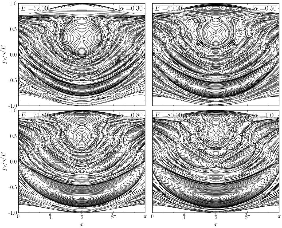
Figure 20: Section $\Sigma$ calculated for energy values at the global maxima energy line, showing the island myriad for different couplings $\alpha$ for the square lattice.

Appendix C Triple folded isochronicity

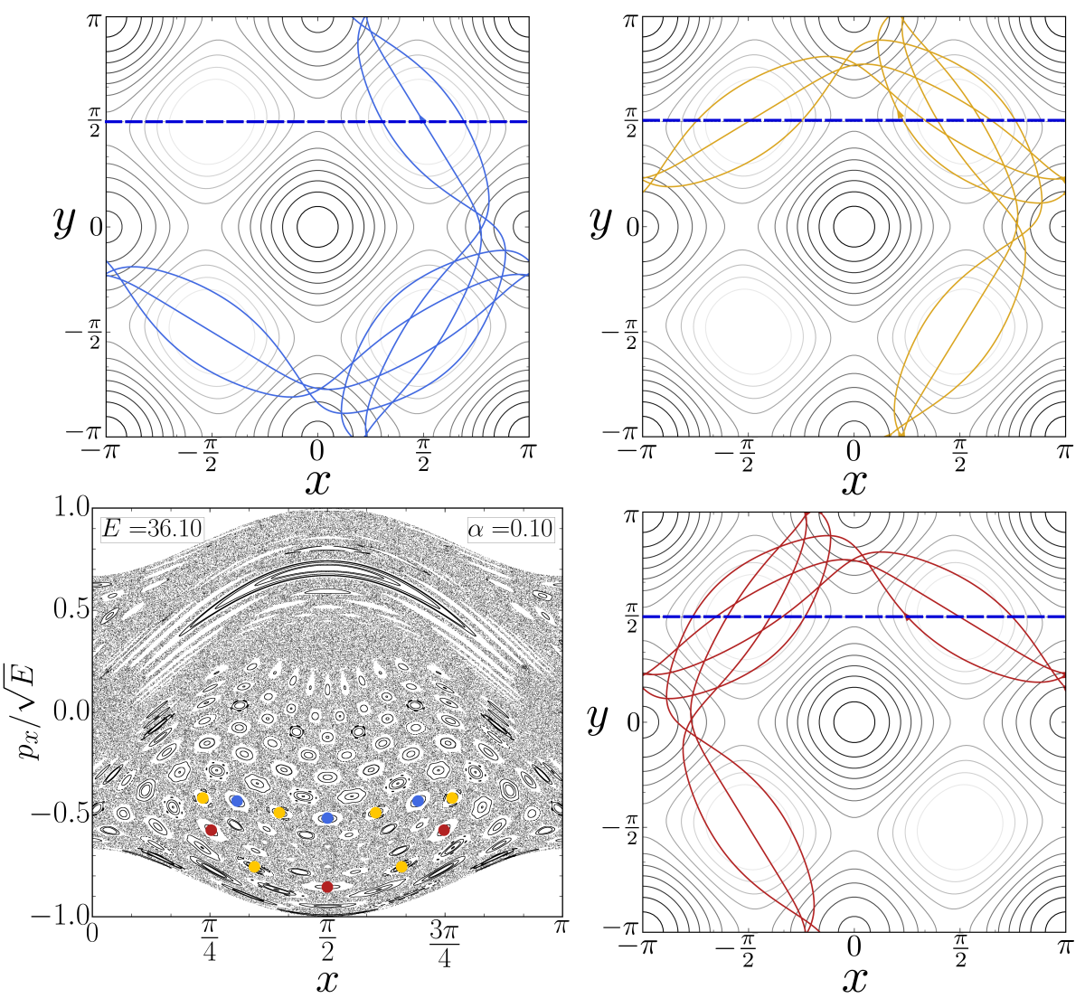
Figure 21: Single myriad chain formed by three isochronous orbits for the square lattice. The colored dots indicate the fixed points of the trajectories relative to the section $\Sigma$ (blue dotted line in trajectory frames).

Figure 21 shows a scenario for the square lattice where a single isochronous chain, with 12 islands, is formed not by two sets of period 6 chains, but instead by two sets of period 3 (shown in red and blue) and one of period 6 (shown in yellow). The orbits themselves show that they are indeed the same curve rotated and mirrored in three different ways, revealing that whenever an orbit’s translation or rotation intersects the Poincaré section with the same discrete period, higher multiplicities may appear. However, for the square lattice, no more than 4 isochronous sets can be expected to appear, since its symmetries are limited by rotations of a quarter of cycle ($\frac{\pi}{2}$).

References

- [1] G. Contopoulos. Order and Chaos in Dynamical Astronomy. Springer, 2002.
- [2] G. H. Walker and J. Ford. Amplitude instability and ergodic behavior for conservative nonlinear oscillator systems. Phys. Rev., 188(1):416–432, 1969.
- [3] D. del Castillo-Negrete; J. M. Green and P. J. Morrison. Area preserving nontwist maps: periodic orbits and transition to chaos. Physica D, 91(1):1–23, 1996.
- [4] L. E. Reichl. The transition to chaos in conservative classical systems. Springer-Verlag, New York, 1992.
- [5] G. M. Zaslavsky; R. Z. Sagdeev; D. K. Chaikovsky and A. A. Chernikov. Chaos and two-dimensional random walk in periodic and quasiperiodic fields. Sov. Phys. JETP, 68(5):995–1000, 1989.
- [6] G. M. Zaslavsky. Hamiltonian chaos and Fractional Dynamics. Oxford University Press, UK, 2005.
- [7] A. A. Chernikov; M. Y. Natenzon; B. A. Petrovichev; R. Z. Sagdeev and G. M. Zaslavsky. Strong changing of adiabatic invariants, KAM-tori and web-tori. Physics Letters A, 129(7):377–380, 1988.
- [8] M. J. Lazarotto; I. L. Caldas and Yves Elskens. Diffusion transitions in a 2d periodic lattice. Communications in Nonlinear Science and Numerical Simulation, 112:106525, 2022.
- [9] I. Bloch. Ultracold quantum gases in optical lattices. Nature Physics, 1:23–30, 2005.
- [10] R. G. Kleva and J. F. Drake. Stochastic ExB particle transport. Physics of Fluids, 27(7):1686–1698, 1984.
- [11] D. S. Sholl and R. T. Skodje. Diffusion of xenon on a platinum surface: the influence of correlated flights. Physica D, 71:168–184, 1994.
- [12] R. Grimm; M. Weidemuller and Y. B. Ovchinnikov. Optical dipole traps for neutral atoms. Advances in Atomic, Molecular and optical physics, 42:95–170, 2000.
- [13] E. Horsley; S. Koppell and L. E. Reichl. Chaotic dynamics in a two-dimensional optical lattice. Physical Review E, 89:012917, 2014.
- [14] M. D. Porter; A. Barr; A. Barr and L. E. Reichl. Chaos in the band structure of a soft Sinai lattice. Physical Review E, 95:052213, 2017.
- [15] C. Skokos; T. Bountis; C. G. Antonopoulos and M. N. Vrahatis. Detecting order and chaos in hamiltonian systems by the SALI method. Journal of Physics A Mathematical and General, 37:6269–6284, 2004.
- [16] G. A. Gottwald C. H. Skokos and J. Laskar. Chaos Detection and Predictability. Springer-Verlag, Berlin Heidelberg, 2015.
- [17] M. C. de Sousa; I. L. Caldas; A. M. Ozorio de Almeida; F. B. Rizzato and R. Pakter. Alternate islands of multiple isochronous chains in wave-particle interactions. Physical Review E, 88:064901, 2013.
- [18] B. B. Leal; I. L. Caldas; M. C. de Sousa; R. L. Viana and A. M. Ozorio de Almeida. Isochronous island bifurcations driven by resonant magnetic perturbations in tokamaks. arXiv, 2308.00810, 2023.
- [19] P. J. Morrison and A. Wurm. Nontwist maps. Scholarpedia, 4(9):3551, 2009.
- [20] C. Baesens; Y-C. Chen and R. S. Mackay. Abrupt bifurcations in chaotic scattering: view from the anit-integrable limit. Nonlinearity, (26):2703–2730, 2013.