Spatio-Temporal Anomaly Detection with Graph Networks for Data Quality Monitoring of the Hadron Calorimeter

Abstract

The compact muon solenoid (CMS) experiment is a general-purpose detector for high-energy collision at the large hadron collider (LHC) at CERN. It employs an online data quality monitoring (DQM) system to promptly spot and diagnose particle data acquisition problems to avoid data quality loss. In this study, we present semi-supervised spatio-temporal anomaly detection (AD) monitoring for the physics particle reading channels of the hadronic calorimeter (HCAL) of the CMS using three-dimensional digi-occupancy map data of the DQM. We propose the GraphSTAD system, which employs convolutional and graph neural networks to learn local spatial characteristics induced by particles traversing the detector, and global behavior owing to shared backend circuit connections and housing boxes of the channels, respectively. Recurrent neural networks capture the temporal evolution of the extracted spatial features. We have validated the accuracy of the proposed AD system in capturing diverse channel fault types using the LHC Run-2 collision data sets. The GraphSTAD system has achieved production-level accuracy and is being integrated into the CMS core production system–for real-time monitoring of the HCAL. We have also provided a quantitative performance comparison with alternative benchmark models to demonstrate the promising leverage of the presented system.

Keywords Anomaly Detection  $\cdot$ Monitoring  $\cdot$ Spatio-Temporal  $\cdot$ Deep Learning  $\cdot$ Graph Networks  $\cdot$ DQM  $\cdot$ CMS  $\cdot$ LHC

Acronyms

AD	Anomaly Detection
CMS	Compact Muon Solenoid
CNN	Convolutional Neural Network
DL	Deep Learning
DQM	Data Quality Monitoring
FC	Fully-Connected Neural Network
GNN	Graph Neural Network
GraphSTAD	Graph Based ST AD model
HCAL	Hadron Calorimeter
HE	HCAL Endcap detector
HEP	High Energy Physics
LHC	Large Hadron Collider
LS	Lumisection
MAE	Mean Absolute Error
MSE	Mean Square Error
QIE	Charge Integrating and Encoding
RBX	Readout Box
RNN	Recurrent Neural Network
SiPM	Silicon Photo Multipliers
ST	Spatio-Temporal
VAE	Variational Autoencoder
$\gamma$	Digi-occupancy
$i\eta$	$ieta$ axis coordinate of the spatial CMS-HCAL channels
$i\phi$	$iphi$ axis coordinate of the spatial CMS-HCAL channels
$depth$	$depth$ axis coordinate of the spatial CMS-HCAL channels

1 Introduction

The large hadron collider (LHC) is the largest particle collider ever built globally. It is designed to conduct experiments in physics and increase our understanding of the universe–with the expectation that new findings will lead to practical applications. The LHC was started in 2008 and consists of a 27 km ring tunnel located 100 meters underground at the France-Switzerland border near Geneva Evans and Bryant (2008). The LHC is a two-ring superconducting hadron accelerator and collider capable of accelerating and colliding beams of protons and heavy ions with the unprecedented luminosity of $10^{34}$ cm^-2s^-1 and $10^{27}$ cm^-2s^-1, respectively, at a velocity close to the speed of light–$3\times 10^{8}$ ms^-1 Evans and Bryant (2008); Heuer (2012). The LHC consists of several experiments on its sites, and its ring holds several detectors for these experiments. The four major detectors of the LHC are a toroidal LHC apparatus (ATLAS), compact muon solenoid (CMS), large hadron collider beauty (LHCb), and a large ion collider experiment (ALICE). Each detector studies particle collisions from a different perspective with different technologies. The ATLAS at point 1 (P1) and the CMS at point 5 (P5) are the two high-luminosity general-purpose detectors at the LHC, and they are located in diametrically opposite sections.

The CMS experiment employs the data quality monitoring (DQM) system to guarantee high-quality physics data through online monitoring that provides live feedback during data acquisition, and offline monitoring that certifies the data quality after offline processing Azzolini et al. (2019). The online DQM identifies emerging problems using reference distribution and predefined tests to detect known failure modes using summary histograms, such as a digi-occupancy map of the calorimeters Tuura et al. (2010); De Guio and Collaboration (2014). A digi-occupancy map contains the histogram record of particle hits of the data-taking channels of the calorimeters. The CMS calorimeters could have several flaws, such as issues with the frontend particle sensing scintillators, digitization and communication systems, backend hardware, and algorithms, which are usually reflected in the digi-occupancy map. The growing complexity of the detector and the variety of physics experimentation make data-driven anomaly detection (AD) systems essential tools for the CMS to identify and localize detector anomalies automatically. Recent efforts in the CMS have proposed deep learning (DL) for AD applications for the DQM Azzolin et al. (2019); Azzolini et al. (2019); Pol et al. (2019a, b). The CMS detector consists of a tracker to reconstruct particle paths accurately, two calorimeters, the electromagnetic (ECAL) and the hadronic (HCAL) to detect electrons, photons, and hadrons, respectively, and of several muon detectors. The synergy in AD has thus far achieved promising results on spatial 2D histogram maps of the DQM for the ECAL Azzolin et al. (2019) and the muon detectors Pol et al. (2019b). Previous studies only considered extreme anomalies, such as dead–no reading–and hot–high noise–particle sensing channels. Detecting degrading channels–essential for quality deterioration monitoring and early intervention–is often overlooked. For instance, the improperly tuned bias voltage on the HCAL physics particle sensing channels caused non-uniformity in the hit map of the DQM, but the channels were neither dead nor hot Viazlo and Collaboration (2022). Calorimeter channels may degrade with subtle abnormality before reaching extreme channel fault status. Capturing such subtle anomalies–e.g., slow system degradation–makes temporal AD models appealing for early anomaly prediction before ultimate system failure. Time-aware models extract temporal context to enhance AD performance. A few efforts have thus far been focused on temporal models despite the acknowledged potential in the future automation technology challenges at the LHC Azzolin et al. (2019); Wielgosz et al. (2018). Our study focuses on DQM automation through time-aware AD modeling using digi-occupancy histogram maps of the HCAL. The digi-occupancy data of the HCAL is 3D, and it poses multidimensional challenges due to its depth-wise calorimeter segmentation; it is relatively unexplored with ML endeavors. The particle hit map data of the HCAL are highly dependent on the collision luminosity–a measure of how many collisions are happening in a particle accelerator–and the number of particles traversing the calorimeter. The effort on data normalization that enhances the learning generalization of machine learning models is still limited.

We address the above gaps while investigating the performance enhancement of temporal AD DL models for the HCAL DQM. We propose to detect anomalies of the HCAL particle sensing channels through a semi-supervised AD system–GraphSTAD–from spatial digi-occupancy maps of the DQM. Anomalies can be unpredictable and come in different patterns of severity, shape, and size–often limiting the availability of labeled anomaly data covering all possible faults. We employ a semi-supervised approach for the AD system; the concept for the AD is that an autoencoder (AE)–trained to reconstruct healthy digi-occupancy maps–would adequately reconstruct the healthy maps, whereas it yields high reconstruction error for maps with anomalies.

Since abnormal events can have spatial appearance and temporal context, we combine both the spatial and temporal features–spatio-temporal (ST)–for AD Xu et al. (2017); Chang et al. (2022); Luo et al. (2019); Hasan et al. (2016); Wu et al. (2020); Hsu (2017); Ullah et al. (2021); Hu et al. (2019); Banković et al. (2012); Zhang et al. (2020). Moreover, modeling the digi-occupancy map of the HCAL is challenging–the spatial nature may exhibit irregularity; although adjacent channels with Euclidean distance are exposed to collision article hits around their region, the channels may belong to different backend circuits–resulting in non-Euclidean spatial behavior on the digi measurements. The GraphSTAD system captures the behavior of channels from regional collision particle hits, and electrical and environmental characteristics due to a shared backend circuit of the channels to effectively detect the degradation of faulty channels. The AD system attains these utilities using a deep AE model that learns local spatial behavior, physical connectivity-induced shared behavior, and temporal behavior through convolutional neural networks (CNN), graph neural networks (GNN), and recurrent neural networks (RNN), respectively.

We have evaluated our proposed AD approach in detecting spatial faults and temporal discords on digi-occupancy maps of the HCAL. We simulated different realistic types of anomalies–dead channels without registered hits, hot channels dominated by electronic noise resulting in a much higher hit count than expected, and degrading channels with deteriorated particle detection efficiency resulting in lower hit counts than expected–to analyze the effectiveness of the AD model. The results have demonstrated promising performance in detecting and localizing the anomalies. We have validated the accuracy in detecting real anomalies and discussed a comparison to the existing DQM system.

In this paper, we briefly describe the DQM and HCAL systems in Section 2, and our data sets in Section 3. Section 4 explains the methodology of the proposed GraphSTAD model, and Section 5 presents the performance evaluation and result discussion. Finally, we summarize the contribution of our study in Section 6.

2 Background

This section describes the CMS DQM and the HCAL systems.

2.1 The Data Quality Monitoring of the CMS Experiment

The particle collision data of the LHC is aggregated into runs, where each run contains thousands of lumisections. A lumisection (LS) corresponds to approximately 23 seconds of data taking and comprises hundreds or thousands of collision events containing particle hit records. The DQM of the CMS provides feedback on detector performance and data reconstruction; It generates a list of certified data for physics analyses–the "Golden JSON" Azzolini et al. (2019). The DQM employs online and offline monitoring mechanisms: 1) the online monitoring is real-time DQM during data acquisition, and 2) the offline monitoring–after 48 hours since the collisions were recorded–provides the final fine-grained data quality analysis for data certification. The online DQM populates a set of histogram-based maps on a selection of events and provides summary plots with alarms that DQM experts inspect to spot problems. The digi-occupancy–one of the histogram maps generated by the online DQM–contains particle hit histogram records of the particle readout channel sensor of the calorimeters. A digi–also called hit–is a reconstructed and calibrated collision physics signal of the calorimeter. Several faults in the calorimeter affecting the frontend particle sensing scintillators, digitalization, communications, the backend hardware, and the algorithms–could appear in the digi-occupancy map. Previous efforts by Azzolin et al. (2019); Azzolini et al. (2019); Pol et al. (2019a, b) demonstrate the promising AD efficacy of using digi-occupancy maps for calorimeter channel monitoring using machine learning. However, end-to-end DL with temporal models are relatively unexplored Azzolin et al. (2019); Pol et al. (2019b).

The purpose of leveraging the DQM through machine learning is to address particular challenges: 1) latency of human intervention, and thresholds require sufficient statistics; 2) the volume of data a human can process in a finite time is limited; 3) rule-based approaches do not scale and assume limited potential failure scenarios; 4) dynamic running conditions change reference samples; 5) the effort to train human shifters who monitor DQM dashboards, and maintain instructions is expensive. Developing machine learning models for the DQM comes with some impediments despite the potential promises; data normalization to handle variation in experimental settings, the granularity of the failures to spot, and limited availability of the ground truth labels are among the challenges Pol et al. (2019b).

We extend the efforts in AD with spatio-temporal (ST) modeling of the digi-occupancy maps of the DQM for the HCAL. Several promising AD models have been proposed in the literature for ST data in non-HEP domains Atluri et al. (2018)–such as crowd monitoring using visual streaming data Xu et al. (2017); Chang et al. (2022); Luo et al. (2019); Wu et al. (2020); Hasan et al. (2016); Ullah et al. (2021); Hu et al. (2019), traffic monitoring Hsu (2017); Deng et al. (2022), cyber-security on sensor systems Banković et al. (2012); Tišljarić et al. (2021); Jiang et al. (2022), medical diagnosis Ahmedt-Aristizabal et al. (2021), and environment monitoring Zhang et al. (2020). A unique quality of ST data that differentiates it from other traditional data studied is the presence of dependencies among measurements induced by the spatial and temporal attributes, where data correlations are more complex to capture by conventional techniques Atluri et al. (2018). Spatio-temporal anomaly is defined as a data point or cluster of data points that violate the nominal ST correlation structure of the normal points Hsu (2017); Deng et al. (2022); Banković et al. (2012); Tišljarić et al. (2021); Xu et al. (2017); Chang et al. (2022); Luo et al. (2019); Wu et al. (2020); Hasan et al. (2016); Ullah et al. (2021); Ahmedt-Aristizabal et al. (2021); Jiang et al. (2022). The previous ST AD studies on video data sets Chang et al. (2022); Luo et al. (2019); Wu et al. (2020); Hasan et al. (2016) focus on CNN models for regular spatial feature extraction, and GNNs are gaining popularity for sensor and traffic flow data Hsu (2017); Deng et al. (2022) that exhibit irregular spatial attributes with non-Euclidean distance among nodes. GNNs have recently achieved promising results at the LHC Duarte and Vlimant (2022); Shlomi et al. (2020), and outperformed CNN in learning irregular calorimeter geometry Qasim et al. (2019) and in pileup mitigation Martínez et al. (2019). The spatial characteristics of the HCAL channels exhibit regular spatial positioning of particle hits in the calorimeter and irregularity in measurement, as adjacent channels may share different backend circuits. Our proposed model integrates both CNN and GNN Bruna et al. (2013); Kipf and Welling (2016) to capture Euclidean and non-Euclidean spatial characteristics, respectively, and RNN for temporal learning for the HCAL channels.

2.2 The Readout Boxes of the HCAL

The HCAL is a specialized calorimeter to capture hadronic particles. The calorimeter is made of multiple subsystems such as HCAL endcap (HE), HCAL barrel (HB), HCAL forward (HF), and HCAL outer (HO) (see Fig. 1).

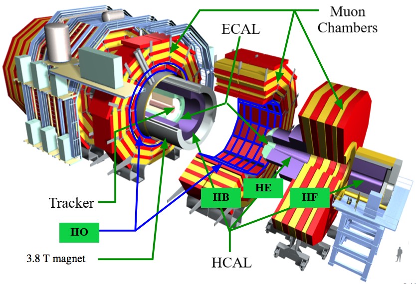
Figure 1: Schematic of the CMS detector at P5 of the LHC and its calorimeters Focardi (2012).

The HCAL frontend electronic systems readout boxes (RBXes) to house the data acquisition electronics. The RBXes provide high voltage, low voltage, backplane communications, and cooling to the data acquisition electronics. The use-case of our study–the HE–is made of 36 RBXes arranged on the plus and minus hemispheres of the CMS. Its frontend particle detection system is built on brass and plastic scintillators, and transmits the produced photon particles through the wavelength-shifting fibers to the Silicon photomultipliers (SiPMs) (see Fig. 2). Each RBX houses four readout modules (RMs) for signal digitization Strobbe (2017); each RM has a SiPM control card, 48 SiPMs, and four readout cards–each includes 12 charge integrating and encoding chips (QIE11) and a field programmable gate array (Microsemi Igloo2 FPGA). The QIE integrates charge from each SiPM at 40 MHz, and the FPGA serializes and encodes the data from the QIE. The encoded data is optically transmitted to the backend system via the CERN versatile twin transmitter (VTTx) at 4.8 Gbps. The current HCAL system has 17 detector scintillator layers that are read out in seven groups–hereafter referred to as $depths$; the light from the scintillators in any given group is optically added together by sending it to a single SiPM. More channels allow for a more refined depth segmentation–ideal for precisely calibrating the depth-dependent radiation damage on the HCAL Azzolini et al. (2019).

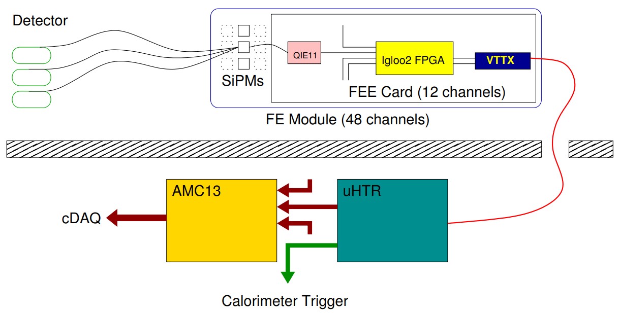
Figure 2: The data acquisition chain of the HE–including the SiPMs, the frontend readout cards, and the optical link connected to the back-end electronics Strobbe (2017). Each readout card contains twelve QIE11 for charge integration, an Igloo2 FPGA for data serialization and encoding, and a VTTx optical transmitter. A fault in the chain may cause anomalous digi-occupancy reading in the online DQM.

3 Data Set Description

We used digi-occupancy map data of the online DQM system of the CMS experiment to train and validate the proposed AD system. The digi-occupancy map data has 3D spatial dimensions with $\eta$ $\phi$, and $depth$ axes, and contains digi histogram records of the calorimeter readout channels referenced by $i\eta=[-32,32]$, $i\phi=[1,72]$ and $depth=[1,7]$ axes (see Fig. 3). The value of the digi-occupancy map varies with the received luminosity–the recorded by the CMS and hereafter referred to as the luminosity–and the number of events–particles traversing the calorimeter–that may differ across LSs. The maps from a sequence of LSs constitute attribution of ST data with correlated spatial and temporal relations Atluri et al. (2018).

We utilized data collected in 2018 during the LHC Run-2 collision experiment. The data set contains about 20K LSs from 20 healthy runs–collected by the CMS experiment–pre-scrutinized by the CMS certifiers, and registered the "Golden JSON" of the DQM as declared of good quality Rapsevicius et al. (2011). The maps–one per LS–were populated with the per LS received luminosity up to 0.4 $pb^{-1}$, and the number of events up to 2250. Our working dataset contains 20K map samples–each with a dimension of $[i\eta=64\times i\phi=72\times depth=7])$.

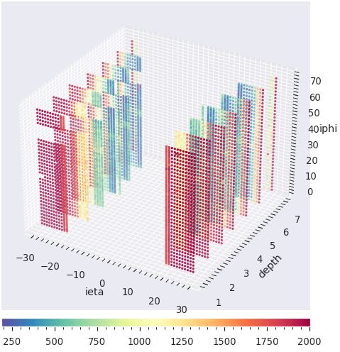
Figure 3: Digi-occupancy map (year=2018, RunId=325170, LS=15) of the HE. The HE channels are placed in $|i\eta|=[14,29]$, $i\phi=[1,72]$, and $depth=[1,7]$. Each pixel in the map corresponds to the readout of a calorimeter channel after a particle hit. The HCAL covers a considerable volume of CMS and has a fine segmentation along three axes ($i\eta$, $i\phi$, and $depth$). The missing section near the top-left of the map is due to two failed RBX (HEM15 and HEM16) sectors during the 2018 collision runs.

4 Methodology

This section presents the proposed GraphSTAD system for online DQM of the HCAL using digi-occupancy map data.

An anomaly is an odd observation from the bulk of observations–often indicating peculiar underlying incidents Chalapathy and Chawla (2019). AD methods can broadly be categorized as supervised or unsupervised: 1) supervised approaches require annotated ground-truth anomaly observations, and 2) unsupervised approaches do not require labeled anomaly data and are more generally pragmatic in many real-world application settings, as data annotation is an expensive task. Unsupervised AD models trained with only healthy observations are called semi-supervised AD approaches.

We present an ST reconstruction AE to detect abnormality in the HCAL channels using reconstruction deviation scores on ST digi-occupancy maps from consecutive lumisections (see Fig. 4). The AE combines CNN, GNN, and RNN to capture ST characteristics of digi-occupancy maps. The spatial feature extraction of the CNNs is leveraged with GNNs to learn circuit and housing connectivity-induced spatial behavior irregularities among the HCAL sensor channels. There are approximately 7K channels–pixels–on the digi-occupancy map of the HCAL endcap subsystem–housed in 36 RBXes. The channels in a given RBX are susceptible to system faults in the RBX due to the shared backbone circuit and environmental factors, such as temperature and humidity. Behavior variations among RBXes have also been observed due to intrinsic deviations of the custom-built electronic components in the RBXes. Our proposed GraphSTAD employs GNNs–in its spatial feature extraction pipeline–to capture the characteristics of the HCAL channels owing to their shared physical connectivity to a given RBX. GNNs have recently achieved promising results in several applications at the LHC Duarte and Vlimant (2022); Shlomi et al. (2020), and outperformed CNN in learning irregular calorimeter geometry Qasim et al. (2019) and in pileup mitigation Martínez et al. (2019). The GraphSTAD system exploits both CNN and GNN Bruna et al. (2013); Kipf and Welling (2016) to capture Euclidean and non-Euclidean spatial characteristics of the HCAL channels, respectively.

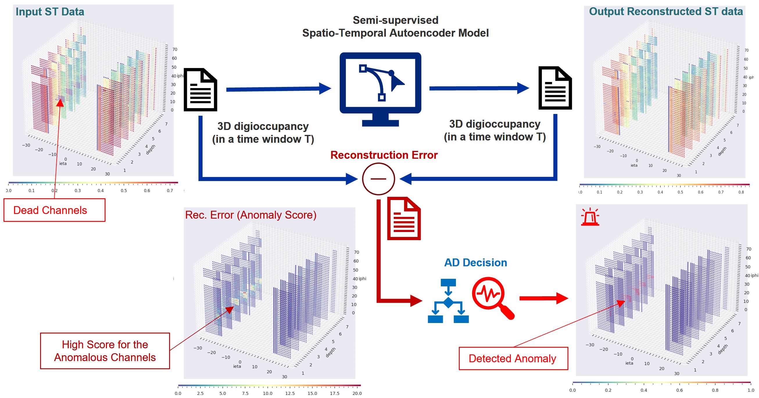
Figure 4: The proposed AE-based reconstruction AD system. The AE reconstructs the input ST digi-occupancy map, and the AD decision is performed on the anomaly scores estimated from the reconstruction errors.

4.1 Data Preprocessing

This section describes the data preprocessing stages of the proposed approach–i.e., digi-occupancy renormalization for particle collision experiment setting variations and graph adjacency matrix generation for the readout channels of the HCAL.

4.1.1 Digi-occupancy Map Renormalization

The digi-occupancy ($\gamma$) map data of the HCAL varies with the received luminosity ($\beta$) and the number of events ($\xi$) (see Fig. 5). We devise a renormalization of the $\gamma$ through a regression model $\mathcal{R}$ to have a consistent quantity interpretation of the $\gamma$ and build a model that robustly generalizes previously unseen run settings–$\beta$ and $\xi$ variations. The $\mathcal{R}$ estimates the renormalizing $\bar{\gamma}_{s}$ at the $s^{th}$ LS using $\beta$ and $\xi$ as:

$$\bar{\gamma}_{s}=\mathcal{R}(\xi,\beta)$$ (1)

The model $\mathcal{R}$ is trained to minimize the MSE cost function, $\mathbb{E}[(\gamma_{s}-\bar{\gamma}_{s})^{2}]$, where $\gamma_{s}$ is calculated as:

$$\gamma_{s}=\sum_{\forall i}\gamma(s,i)$$ (2)

where the $\gamma(s,i)$ is the digi-occupancy of the $i^{th}$ channel in the map at the $s^{th}$ LS. Finally, the per-channel $\gamma(s,i)$ is renormalized by its corresponding $\bar{\gamma}_{s}$ as:

$$\hat{\gamma}(s,i)=\frac{K\gamma(s,i)}{\bar{\gamma}_{s}}$$ (3)

where the $\hat{\gamma}$ is the renormalized $\gamma$, and the $K$ is a scaling factor to compensate for the difference in the number of channels on the depth axes.

We have employed fully connected ($\operatorname{FC}$) neural networks to build the regression model to effectively capture the non-linear relationships illustrated in Fig. 5:

$$input(\xi,\beta)\operatorname{\to ReLU(FC(64))\to ReLU(FC(64))\to ReLU(FC(64))\to}output(\bar{\gamma}_{s})$$ (4)

Fig. 6 depicts data distribution of the $\gamma_{s}$ before and after renormalization with $\mathcal{R}$. The renormalization has successfully handled the discrepancies on the $\gamma_{s}$ from several runs–overlaps and centers distributions of $\hat{\gamma}_{s}$ and minimizes the outliers.

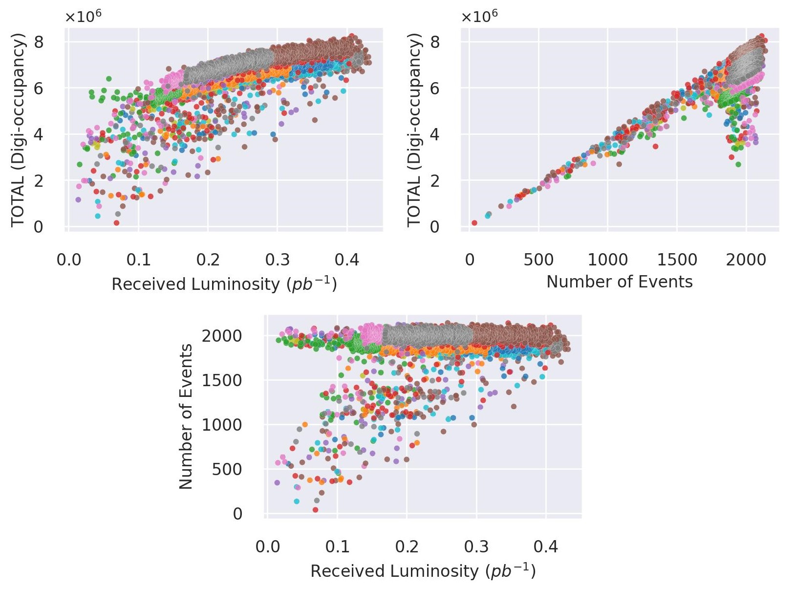
Figure 5: Dependency between digi-occupancy and run settings–the received luminosity and the number of events–in LS granularity. The number of events did not fully follow the drop in the luminosity (right-side plot) and the digi-occupancy (middle plot); it portrays the non-linear behavior of LHC. The different colors correspond to different collision runs.

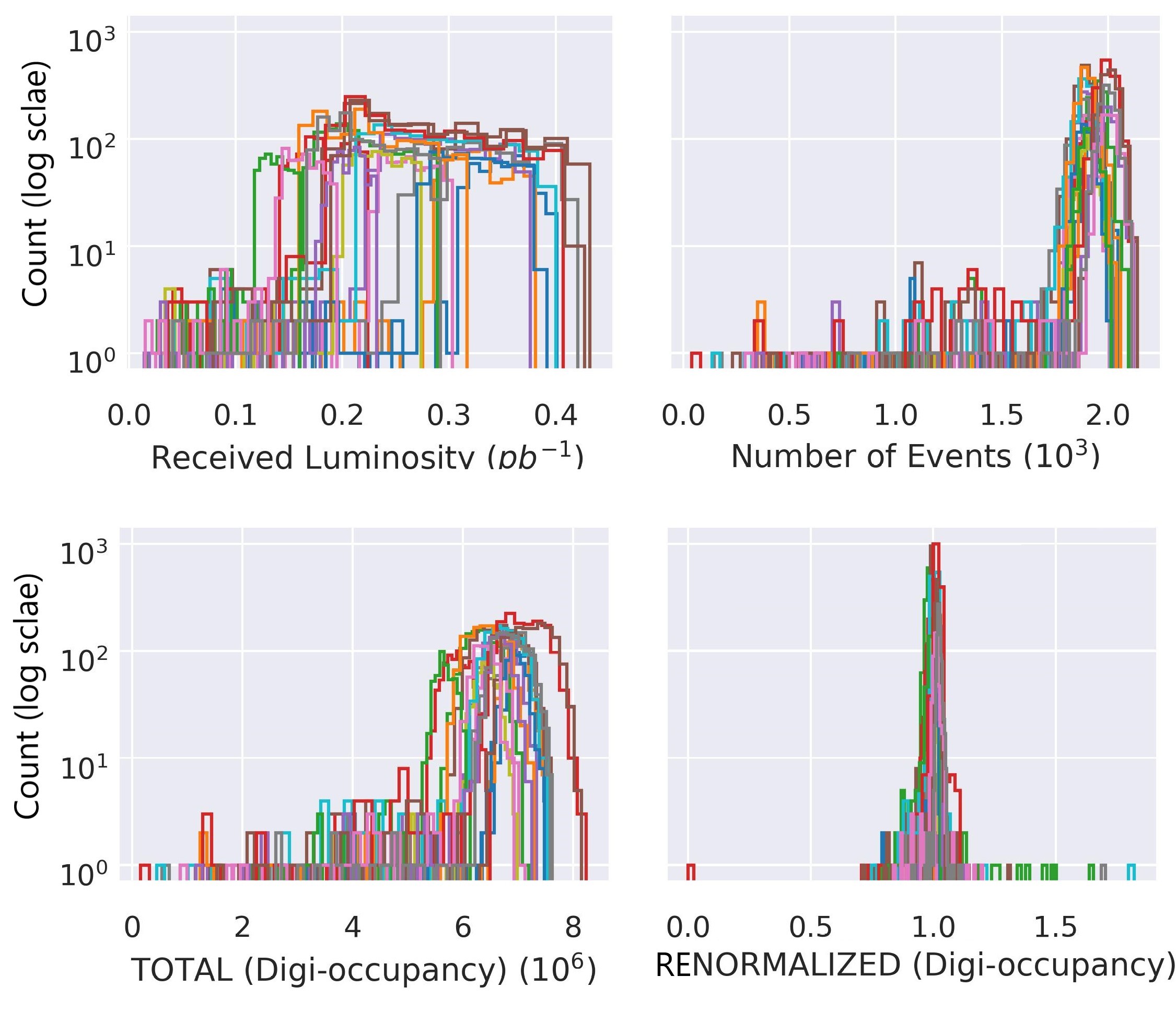
Figure 6: Distribution of total digi-occupancy per LS before and after renormalization. From left to right: a) the received luminosity, b) the number of events, c) the digi-occupancy, and d) the renormalized digi-occupancy obtained with the regression model described in the text. The different colors correspond to different runs.

4.1.2 Adjacency Matrix Generation for Graph Network

We deploy an undirected graph network $\mathcal{G}(\mathcal{V},\Theta)$ to represent the HCAL channels in a graph network based on their connection to a shared RBX system. The graph $\mathcal{G}$ contains nodes $\upsilon\in\mathcal{V}$, with edges $(\upsilon_{i},\upsilon_{j})\in\Theta$ in a binary adjacency matrix $\mathcal{A}\in\mathbb{R}^{M\times M}$, where $M$ is the number of channel nodes. An edge indicates the channels sharing the same RBX as:

$$A(\upsilon_{i},\upsilon_{j})=\begin{cases}1,&\text{if }\Omega(\upsilon_{i})=\Omega(\upsilon_{j})\\ 0,&\text{otherwise}\end{cases}$$ (5)

where $\Omega(\upsilon)$ returns the RBX ID of the channel $\upsilon$.

There are approximately 7K channels in a graph representation of the digi-occupancy map of the HE, where each RBX network contains roughly 190 nodes. We retrieved the channel to RBX mapping from the HCAL’s calorimeter segmentation map.

4.2 Anomaly Detection Modeling

We denote the AE model of the GraphSTAD system as $\mathcal{F}$. The ST data is $\mathrm{X}\in\mathbb{R}^{T\times N_{i\eta}\times N_{i\phi}\times N_{d}\times N_{f}}$ as a sequence in a time window $t_{x}\in[t-T,t]$, where $N_{i\eta}\times N_{i\phi}\times N_{d}$ is the spatial dimension corresponding to the $i\eta$, $i\phi$, and $depth$ axes, respectively, and $N_{f}=1$ is the number of input variables–only a digi-occupancy quantity in the spatial data. The $\mathcal{F}_{\theta,\omega}:\mathrm{X}\to\bar{\mathrm{X}}$–parameterized by $\theta$ and $\omega$–attempts to reconstruct the input ST data $\mathrm{X}$ and outputs $\bar{\mathrm{X}}$. The encoder network of the model $E_{\theta}:\mathrm{X}\to\mathbf{z}$ provides low-dimension latent space, $\mathbf{z}=E_{\theta}(\mathrm{X})$, and the decoder $D_{\omega}:\mathbf{z}\to\bar{\mathrm{X}}$, reconstructs the ST data from $\mathbf{z}$, $\bar{\mathrm{X}}=D_{\omega}(\mathbf{z})$ as:

$$\bar{\mathrm{X}}=\mathcal{F}(\mathrm{X})=D_{\omega}(E_{\theta}(\mathrm{X}))$$ (6)

The channel anomalies can be transients–live short and impact only a single digi-occupancy map–or persist over time–affecting a sequence of maps. The spatial reconstruction error $e$ is calculated to detect a transient anomaly as:

$$e_{i}=|x_{i}-\bar{x}_{i}|$$ (7)

where $x_{i}\in\mathrm{X}$ and $\bar{x}_{i}\in\bar{\mathrm{X}}$ are the input and reconstructed digi-occupancy of the $i^{th}$ channel. The $e_{i}$ detects channel abnormality occurrence on isolated maps. We engage an aggregated error in a time window $T$ using mean absolute error (MAE) to capture a time-persistent anomaly as:

$$e_{i,MAE}=\frac{1}{T}\sum^{t}_{t^{\prime}=t-T}e_{i}(t^{\prime})$$ (8)

We standardize $e_{i}$ to regularize the reconstruction accuracy variations among the channels–allowing a single AD decision threshold $\alpha$ to all the channels in the spatial map–as:

$$a_{i}=\frac{e_{i}}{\sigma_{i}}$$ (9)

where $\sigma_{i}$ is the standard deviation of the $e_{i}$ (or $e_{i,MAE}$ if the time window is considered) on the training dataset. The anomaly flags are generated after applying $\alpha$ to the anomaly scores a $a_{i}>\alpha$. The $\alpha$ is a tunable constant that controls the detection sensitivity.

4.3 Autoencoder Model Architecture

Convolutional neural networks have achieved state-of-the-art performance in several AD DL applications with image data Chang et al. (2022); Luo et al. (2019); Hasan et al. (2016); Hsu (2017); Wu et al. (2020). The shared nature of the kernel filters of the CNNs substantially reduces the number of trainable parameters in the model compared to fully connected neural networks. Directly supplying the learned spatial features into an architecture that can learn temporal data–such as RNN–could become inherently challenging due to the considerable computational demand for high-dimensional data. We employ CNN and GNN with a pooling mechanism to extract relevant features from high dimensional spatial data followed by RNN to capture temporal characteristics of the extracted features (see Fig. 7). We integrate variational layer Kingma and Welling (2013) at the end of the encoder for regularization of AE overfitting by enforcing continuous and normally distributed latent representations Asres et al. (2021); Guo et al. (2018); An and Cho (2015); Chadha et al. (2019).

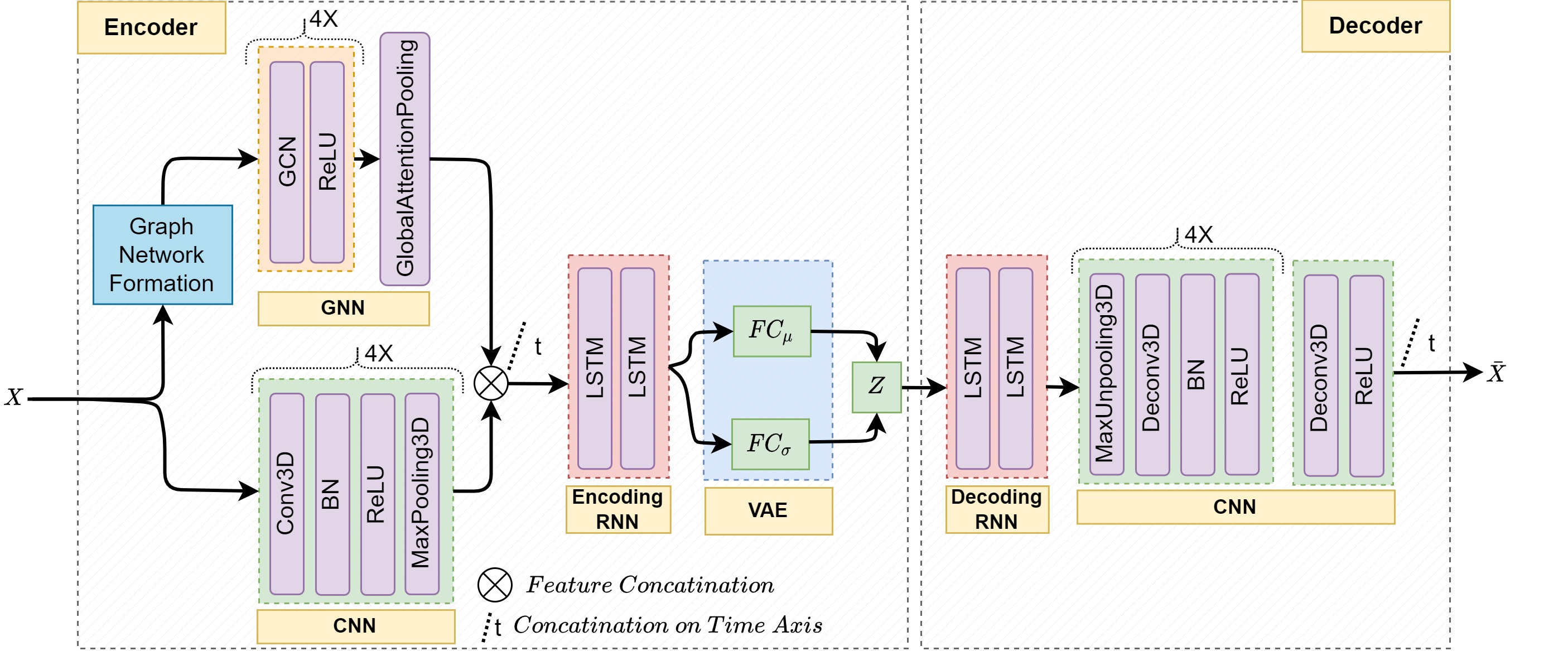
Conv3D: 3D convolutional neural network; GCN: graph convolutional neural networks; Deconv3D: 3D deconvolutional neural networks; BN: batch normalization; LSTM: long short time memory recurrent networks; FC: fully connected neural networks.

Figure 7: The architecture of the proposed AE for the GraphSTAD system. The GNN and CNN are spatial feature extraction on each time step, and the RNN network captures the temporal behavior of the extracted features. The encoder–feature extraction–incorporates the GNN for backend physical connectivity among the spatial channels, CNN for regional spatial proximity of the channels, and RNN for temporal behavior extraction. The decoder–reconstruction–contains RNN and deconvolutional neural networks to reconstruct the spatio-temporal input data from the low dimensional latent features.

The CNN of the encoder has $L_{c}$ networks–each containing $\operatorname{Conv3D(\cdot,kernel\_size=[3\times 3\times 3])}$ for regular spatial learning followed by batch normalization ($\operatorname{BN}$) for network weight regularization and faster convergence, $\operatorname{ReLU}$ for nonlinear activation, and $\operatorname{MaxPooling3D}$ for spatial dimension reduction. The model can be summarized as:

$$y^{c}_{t},\psi^{c}_{t}=\operatorname{Pool}(\operatorname{ReLU}(\operatorname{BN}(\operatorname{Conv3D}(x_{t}^{l},N_{c}^{l}))|_{l=1,...,L_{c}}$$ (10)

where $x_{t}^{l}$ is the input spatial $\gamma$ map data at time-step $t$ and the $N_{c}^{l}$ is the feature size of the $l^{th}$ network. The $y^{c}_{t}$ is the extracted feature set of the CNN at $t$. The $\operatorname{Pool}(\cdot)$ denotes $\operatorname{MaxPooling3D}(\cdot,stride=[2\times 2\times 2])$. The $\psi^{c}_{t}$ holds the pooling spatial location indices of the $\operatorname{MaxPooling3D}$ layers to be used later for upsampling in the decoder during map reconstruction. The final extracted feature set $\mathrm{Y}_{c}\in\mathbb{R}^{T\times N_{c}}$ of the CNN is an aggregation of all $y^{c}_{t}$ in the time window $T$–concatenated on the time dimension–as:

$$\mathrm{Y}_{c}=[y^{c}_{1},y^{c}_{2},...,y^{c}_{T}]$$ (11)

We have used $L_{c}=4$ to map the input spatial dimension $[64\times 72\times 7]$ into $[4\times 4\times 1]$, which yields a reduction factor of $2^{L_{c}}$ and expands the feature space of the input from $N_{f}=1$ to $N_{c}=128$. The $N^{\prime}_{c}:[4\times 4\times 1\times 128]=2048$ spatial features are generated after reshaping.

The GNN of the encoder has $L_{g}$ networks of a graph convolutional network ($\operatorname{GCN}$) with $\operatorname{ReLU}$ activation, and a final global attention pooling. The networks are summarized as:

$$\begin{gathered}y^{g}_{t}=\operatorname{Pool}(\operatorname{ReLU}(\operatorname{GCN}(x_{t}^{l},N_{g}^{l})|_{l=1,...,L_{g}}))\\ \mathrm{Y}_{g}=[y^{g}_{1},y^{g}_{2},...,y^{g}_{T}]\end{gathered}$$ (12)

where the $\operatorname{GCN}$ layers have a feature size of $N_{g}^{l}$, and the $\operatorname{Pool}(\cdot)$ signifies the $\operatorname{GlobalAttentionPooling}(\cdot)$ at the end of the GNN. The $\operatorname{GlobalAttentionPooling}$ aggregates the graph node features with an attention mechanism to obtain the final feature set of the GNN $\mathrm{Y}_{g}\in\mathbb{R}^{T\times N_{g}}$. Similar to the CNN, we set $L_{g}=4$ and $N_{g}=128$ to generate the $\mathrm{Y}_{g}$.

The encoded ST feature set $\zeta\in\mathbb{R}^{1\times N_{z}}$ is obtained by learning the temporal context on the extracted spatial features $\mathrm{Y}=[\mathrm{Y}_{c},\mathrm{Y}_{g}]$ with two layers of long short-time memory ($\operatorname{LSTM}$) as:

$$\zeta=\operatorname{LSTM}(\mathrm{Y},N^{l}_{r})|_{l=1,2}$$ (13)

where $N^{l}_{r}$ is the feature size of the $l^{th}$ LSTM layer. The last layer ($N^{2}_{r}=N_{z}=32$) generates the low-dimensional latent representation of the encoder. The VAE layer of the encoder generates the normally distributed representation latent features $\mathbf{z}$ as:

$$\begin{gathered}\mathbf{z}=\mu_{z}+\sigma_{z}\odot\epsilon\end{gathered}$$ (14)

where $\odot$ signifies an element-wise product with standard normal distribution sampling $\epsilon\sim\mathcal{N}(0,1)$ An and Cho (2015). The $\mu_{z}$ and the $\sigma_{z}$ of the VAE are implemented with $\operatorname{FC}$ layers taking the $\zeta$ as input.

The decoder network of the AE is made of RNN and CNN to reconstruct the target ST data from the latent features. The decoding embarks with temporal feature reconstruction using $\operatorname{LSTM}$ network as:

$$\bar{\zeta}=\operatorname{LSTM}(\mathbf{z},N_{r}^{l})|_{l=1,2}$$ (15)

where $\bar{\zeta}$ is the reconstructed temporal feature set from the latent space $\mathbf{z}$. Spatial reconstruction follows for each time-step $t$ through a multi-layer deconvolutional neural network. Each network starts with $\operatorname{MaxUnpooling3D}(\cdot,stride=[2\times 2\times 2],\psi^{c}_{l})$ to upsample the spatial data using localization indices $\psi^{c}_{l}$ from the $l^{th}$ $\operatorname{MaxPooling3D}$ of the encoder followed by a deconvolutional layer ($\operatorname{Deconv3D(\cdot,kernel\_size=[3\times 3\times 3])}$) Zeiler et al. (2010), $\operatorname{BN}$ and $\operatorname{ReLU}$. Eventually, $\operatorname{Deconv3D(\cdot,kernel\_size=[1\times 1\times 1])}$ is incorporated for final output stabilization. The decoder network is summarized as:

$$\begin{gathered}\bar{x}_{t}=\operatorname{ReLU}(\operatorname{BN}(\operatorname{Deconv3D}(\operatorname{Unpool}(\bar{\zeta_{t}},\psi^{c}_{t}),N_{c}^{l}))|_{l=1,...,L_{c}}\\ \bar{x}_{t}=\operatorname{ReLU}(\operatorname{Deconv3D}(\bar{x}_{t},N_{f}))\end{gathered}$$ (16)

where the $\bar{x}_{t}$ is the reconstructed spatial data, and the $\operatorname{Unpool}(\cdot)$ denotes $\operatorname{MaxUnpool3D}(\cdot)$. The final reconstructed ST data $\bar{\mathrm{X}}\in\mathbb{R}^{T\times N_{i\eta}\times N_{i\phi}\times N_{d}\times N_{f}}$ is obtained as:

$$\bar{\mathrm{X}}=[\bar{x}_{1},\bar{x}_{2},...,\bar{x}_{T}]$$ (17)

4.4 Model Training

We trained the AE on healthy digi-occupancy maps of LHC collision runs (described in Section 3). The modeling task becomes a multivariate learning problem since the target data contains readings from multiple calorimeter channels in the spatial digi-occupancy map. Appropriate scaling of the spatial data is thus necessary for effective model training; we further normalized the spatial data per channel into a range of $[0,1]$. We have also observed that the $\gamma$ distribution of the channels at the first depth of the spatial map is different from the channels at the higher depths (see Fig. 3); distribution imbalance on target channel data affects model training efficacy when well-known statistical algorithms, such as MSE, are employed as loss functions. MSE loss minimizes the cost of the entire space, and it may converge to a non-optimal local minimum in the presence of imbalanced data distribution; this phenomenon is known as the class imbalance challenge in machine learning classification problems. A popular remedy is to employ a weighting mechanism–assigning weights to the different targets. We applied a weighted MSE loss function to scale the loss from the different distributions–the $depth\in{1}$ and $depth\in{2,\dots,7}$–as:

$$\mathcal{L}^{\prime}=\sum_{j}\frac{\varsigma_{j}}{M_{j}}\sum_{i\in C_{j}}(x_{i}-\bar{x}_{i})^{2}$$ (18)

where $x_{i}$ is the $\hat{\gamma}$ of the $i^{th}$ channel in the $j^{th}$ group set $C_{j}$, $M_{j}$ is the number of channels in $C_{j}$, and $\varsigma_{j}$ is the weight factor of the MSE loss of the $j^{th}$ group. We holistically set $\varsigma_{1}=0.4$ and $\varsigma_{2}=1$ after experimenting with several different $\varsigma$ values.

The VAE regularizes the training MSE loss using the KL divergence loss $D_{KL}$ to achieve the normally distributed latent space as:

$$\mathcal{L}=\underset{W\in\mathbb{R}}{\text{argmin}}\left\{\mathcal{L}^{\prime}-\lambda{D_{KL}}\left[\mathcal{N}(\mu_{z},\sigma_{z})\|\mathcal{N}(0,I)\right]+\rho\|W\|_{2}^{2}\right\}$$ (19)

where $\mathcal{N}$ is a normal distribution with zero mean and unit variance, and $\|.\|$ is the Frobenius norm of $L_{2}$ regularization for the trainable model parameters $W$. The $\lambda=0.003$ and $\rho=10^{-7}$ are tunable regularization hyperparameters. We finally used Adam optimizer with super-convergence one-cyclic learning rate scheduling Smith and Topin (2019) for training.

5 Results and Discussion

In this section, we discuss the AD performance of the proposed GraphSTAD on simulated and real anomalies.

The ML studies for the CMS DQM mostly inject simulated anomalies into good data to validate the effectiveness of the developed models Azzolin et al. (2019) since a small fraction of the data is affected by real anomalies. We trained the AE model on 10K digi-occupancy maps–from LS sequence number $[1,500]$–and evaluated on LSs $[500,1500]$ injected with synthetic anomalies simulating real dead, hot, and degrading channels. We trained the AE on four GPUs with early-stopping using 20% of the training dataset to estimate the validation loss during each training epoch.

Fig. 8 demonstrates the capability of the proposed ST AE in reconstructing normal digi-occupancy maps from a sequence of lumisections. The AE has accomplished a promising reconstruction ability on the ST digi-occupancy data. High reconstruction accuracy on the healthy data is essential to reduce false-positive flags when a semi-supervised AE is employed for AD application. We further discuss the reconstruction error distribution comparison on the healthy and abnormal channels in the AD performance in Section 5.1.2.

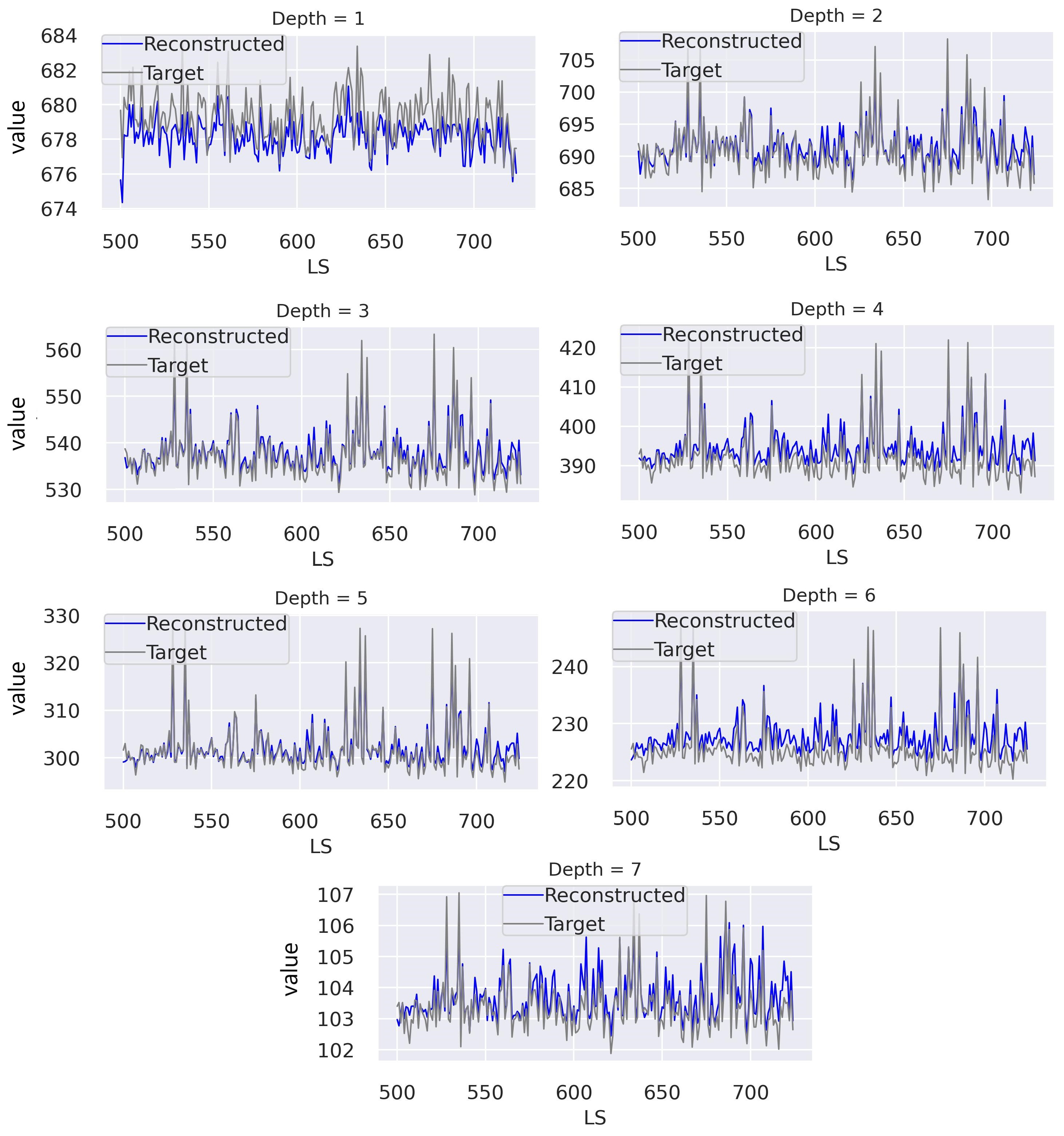
Figure 8: ST digi-occupancy maps reconstruction on samples from the test dataset (RunId: 325170, LS=[500, 750]). The figure illustrates the total digi-occupancy per LS across the seven depths ($\hat{\gamma}_{l}$). The proposed GraphSTAD AE operates on ST $\gamma$ map data, and we present the curves corresponding to the $\gamma_{l}$ per LS only to demonstrate the capability of the AE in handling the fluctuation across the sequence of lumisections.

We will discuss below the AD performance of the proposed system and comparisons with benchmark models, and present the detection of real faulty channels to demonstrate the accuracy of the proposed approach.

5.1 Anomaly Detection Performance

We generated synthetic anomalies simulating real dead, hot, and degrading channels and injected them into healthy digi-occupancy maps; the anomaly generation algorithm involves three steps: 1) selection of a random set of LSs from the test set, 2) random selection of spatial locations $\varphi$ for each LS, where $\varphi\in\{i\eta\times i\phi\times depth\}$ on the HE axes (see Fig. 3), and 3) injection of anomalies such as dead ($\gamma_{anomaly}=0$), hot ($\gamma_{anomaly}>>\gamma_{expected}$), and degrading channels ($0\leq\gamma_{anomaly}<\gamma_{expected}$) into digi-occupancy maps of the LSs. We have kept the same spatial locations of the generated anomalies for consistency when evaluating the AD performance of the different anomaly types.

5.1.1 Detection of Dead and Hot Channels

We have evaluated the AD accuracy on dead–$\gamma_{a}=0$–and hot–$\gamma_{a}=200\%\gamma_{h}$–channels on the 10K maps–5K maps for each anomaly type. We have investigated the AD performance on transient channel anomalies that are short-lived in isolated maps (see Table 1) and persisting anomalies that encroach consecutive maps in a time window (see Table 2). The model has achieved high accuracy with good localization of the faulty channels–0.99 precision when capturing 99% of the 335K faulty channels. Time-persistent anomalies are easier to detect–the FPR generally improves by 13%-23% and 28%-40% for the dead and hot anomalies, respectively–compared to the short-lived anomalies on isolated LSs. We have observed that most FPs occur on channels with low expected $\gamma$, where the model achieves relatively lower reconstruction accuracy. The performance is not entirely unexpected, as we trained the AE to minimize a global MSE loss function (19). The reconstruction errors become relatively higher for channels with low $\gamma$ ranges that limit AD effectiveness in distinguishing the anomalies when capturing 99% of the time-persistent dead channels using (8).

We have monitored roughly 31.28M HE sensor channels–of which 335K (1.07%) are simulated abnormal channels–from the 5K maps on the isolated map evaluation in Table 1. The monitored channels grow to 156M with 1.68M (1.07%) anomalies for the evaluation of time-persistent anomalies in Table 2 using time window five maps resulting in 25K maps.

Table 1: AD on dead and hot channel anomalies on isolated digi-occupancy maps.

Anomaly Type	Captured Anomalies	P	R	F1	FPR
Dead Channel ($R_{D}=0\%$)	99%	$0.999$	$0.99$	$0.995$	$6.722\times 10^{-6}$
	95%	$1.000$	$0.95$	$0.974$	$3.102\times 10^{-6}$
	90%	$1.000$	$0.90$	$0.947$	$2.068\times 10^{-6}$
Hot Channel ($R_{D}=200\%$)	99%	$0.999$	$0.99$	$0.994$	$9.113\times 10^{-6}$
	95%	$1.000$	$0.95$	$0.974$	$1.939\times 10^{-6}$
	90%	$1.000$	$0.90$	$0.947$	$1.196\times 10^{-6}$

^* P – Precision, R – Recall, F1 – F1-score, and FPR – False Positive Rate

Table 2: AD on time-persistent dead and hot channel anomalies.

Anomaly Type	Captured Anomalies	P	R	F1	FPR
Dead Channel ($R_{D}=0\%$)	99%	$0.999$	$0.99$	$0.995$	$7.691\times 10^{-6}$
	95%	$1.000$	$0.95$	$0.974$	$2.715\times 10^{-6}$
	90%	$1.000$	$0.90$	$0.947$	$1.616\times 10^{-6}$
Hot Channel ($R_{D}=200\%$)	99%	$0.999$	$0.99$	$0.995$	$5.461\times 10^{-6}$
	95%	$1.000$	$0.95$	$0.974$	$1.357\times 10^{-6}$
	90%	$1.000$	$0.90$	$0.947$	$7.756\times 10^{-7}$

5.1.2 Detection of Degrading Channels

Table 3 presents the AD accuracy of time-persistent degrading channels simulated with $R_{D}=[80\%,60\%,40\%,20\%,0\%]$; the $R_{D}=0\%$ corresponds to a dead channel. We injected the generated channel faults into 1K maps for each decay factor. We have monitored around 156M channels–of which 1.74M (1.11%) are abnormal channels–in the total of 25K digi-occupancy maps–5K maps per in the time window. The AD system has demonstrated promising potential in detecting degraded channel anomalies. The FPR to capture 99% of the anomaly is 2.988%, 0.155%, 0.022%, 0.002%, and 0.001% when channels operate at 80%, 60%, 40%, 20%, and 0% of their expected capacity, respectively.

The relatively lower precision at the $R_{D}=80\%$ indicates that there are still a few anomalies challenging to catch even though the FPR is very low considering the accurate classification of numerous TN healthy channels (see Fig. 9); The channels operating at $R_{D}=80\%$ are mostly inliers–overlapping with the healthy operating ranges–and detecting such anomalies is difficult when the expected $\gamma$ of the channel is low. The significant improvement of the FPR by 88% and 95% when the amount of the captured anomaly is reduced to 95% and 90%, respectively, demonstrates a small percentage of the channels causes the performance drop at $R_{D}=80\%$. Fig. 10 illustrates the overlap regions on the distribution of the reconstruction errors of the healthy and faulty channels at the various $R_{D}$ values.

Table 3: AD on time-persistent degrading channels.

Anomaly Type	Health Rate	FPR (90%)	FPR (95%)	FPR (99%)
Degrading Channel	80%	$1.636\times 10^{-3}$	$3.614\times 10^{-3}$	$2.988\times 10^{-2}$
	60%	$1.329\times 10^{-4}$	$3.834\times 10^{-4}$	$1.550\times 10^{-3}$
	40%	$8.405\times 10^{-6}$	$2.764\times 10^{-5}$	$2.242\times 10^{-4}$
	20%	$2.263\times 10^{-6}$	$5.173\times 10^{-6}$	$2.505\times 10^{-5}$
	0%	$9.699\times 10^{-7}$	$1.778\times 10^{-6}$	$6.142\times 10^{-6}$

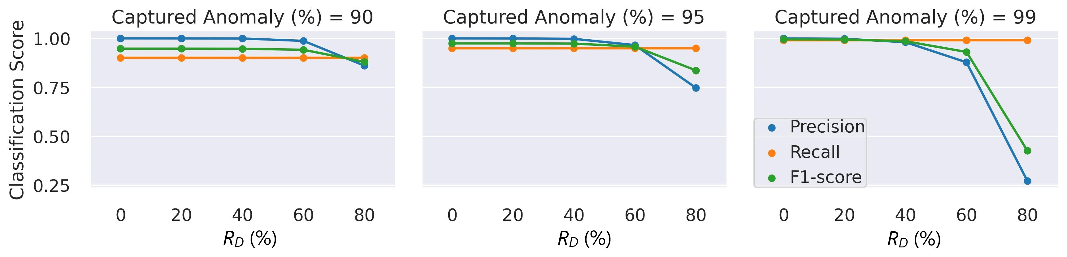
Figure 9: AD classification performance on time-persistent degrading channels.

Figure 10: Reconstruction error distribution of healthy and anomalous channels at different health rates. The overlap region decreases substantially as the channel deterioration increases (left to right).

5.1.3 Performance Comparison with Benchmark Models

We have quantitatively compared alternative benchmark models to validate the capability of the GraphSTAD (see Fig. 11). The benchmark AE models employ a similar architecture as the GraphSTAD AE but with different layers. The results demonstrate that the integration of the GNN has a significant performance improvement from 1.6 to 3.9 times in the FPR. The temporal models–with RNN–have achieved a 3 to 5-fold boost over the non-temporal spatial AD model when capturing severely degraded channels. For subtle or inlier anomalies–e.g., when channels deteriorate by 20% at $R_{D}=80\%$–the GraphSTAD has a substantial 25 times amelioration over the non-temporal model. Incorporating temporal modeling and GNN has enhanced degrading channel detection performance.

CNN: convolutional neural network, GNN: graph neural network, BiLSTM: bidirectional LSTM, GRU: gated recurrent unit, and VAE: variational AE.

Figure 11: Comparison with benchmark models on detecting time-persistent degrading channels. The GraphSTAD model achieves a significantly lower FPR.

5.1.4 Detection of Real Anomalies in the HCAL

The GraphSTAD system has spotted five real faulty HE channels in collision data RunId=324841 using the digi-occupancy maps The faulty channels are located at $[i\eta=17,i\phi=71,depth=3]$, $[i\eta=18,i\phi=71,depth=3]$, $[i\eta=18,i\phi=71,depth=4]$, $[i\eta=18,i\phi=71,depth=5]$, and $[i\eta=28,i\phi=71,depth=4]$, and have impacted 52 consecutive LSs (see Fig. 12). Fig. 12 and Fig. 13 illustrate the detected faults fall into the dead channel category except in the last LS=57 where the channels operated in a degraded state–the $\gamma$ is lower than expected. Detecting degraded channels is challenging since the $\gamma$ reading is non-extreme like in dead and hot channels, and the $\gamma$ drop overlaps with other false down-spikes (see LS $>$ 57 in Fig. 12). The down-spikes in the digi-occupancy for LS $>$ 57 are due to non-linearity in the LHC–changes in collision run settings (see Fig. 12(b)); our normalizing regression model has successfully handled the fluctuation during prepossessing before causing false-positive alerts (see Fig. 12(a)). Fig. 14 and Fig. 15 portray the spatial anomaly scores during death and degraded status of the faulty channels; the high anomaly scores localized at the faulty channels demonstrate the GraphSTAD AD performance at a channel-level granularity. The existing production DQM system of the CMS–uses rule-based and statistical methods–has also reported these abnormal channels at run-level analysis; the results are only available at the end of the run after analyzing all the LSs for the run Tuura et al. (2010). Our approach is adaptive to variability in the digi-occupancy maps and provides anomaly localization that detects faulty–including non-extreme degrading–channels per lumisection granularity.

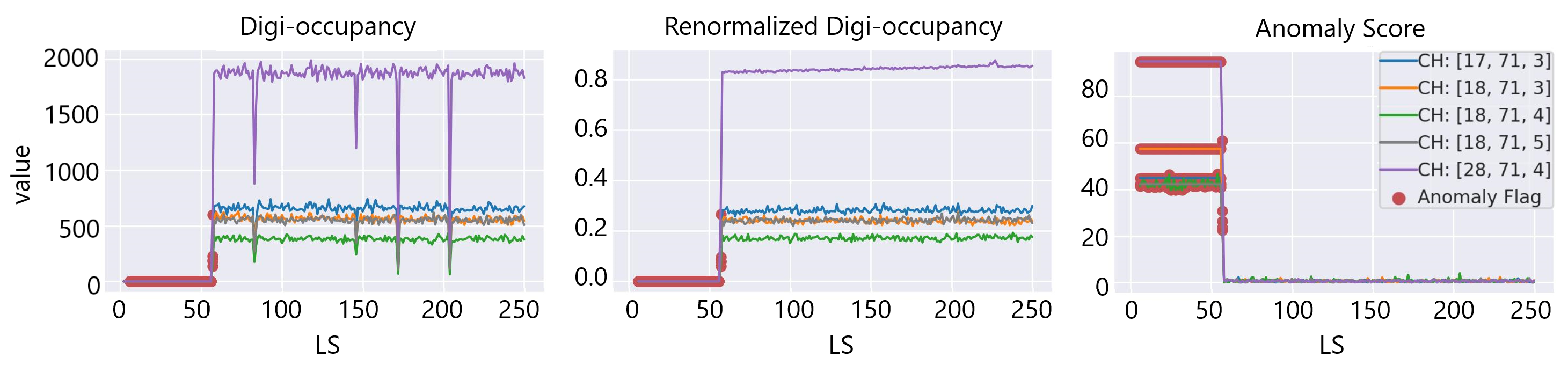
((a))

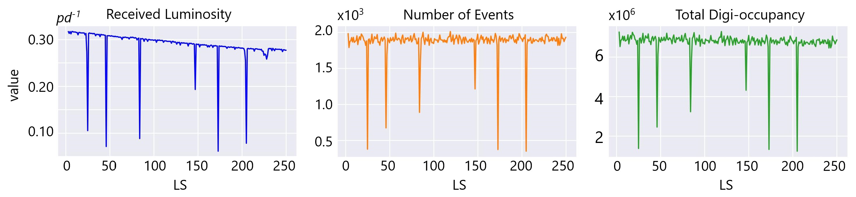
((b))

Figure 12: Detected real faulty channels on digi-occupancy maps at LS=[6, 57] of RunId=324841. (a) The digi-occupancy dropped to near zero for the faulty channels (left and middle plots), resulting in high anomaly scores (right). Dead (LS=[6, 56]) and degraded channel anomalies (LS=57) were captured on the highlighted LSs (red). (b) collision run settings and the total digi-occupancy per LS.

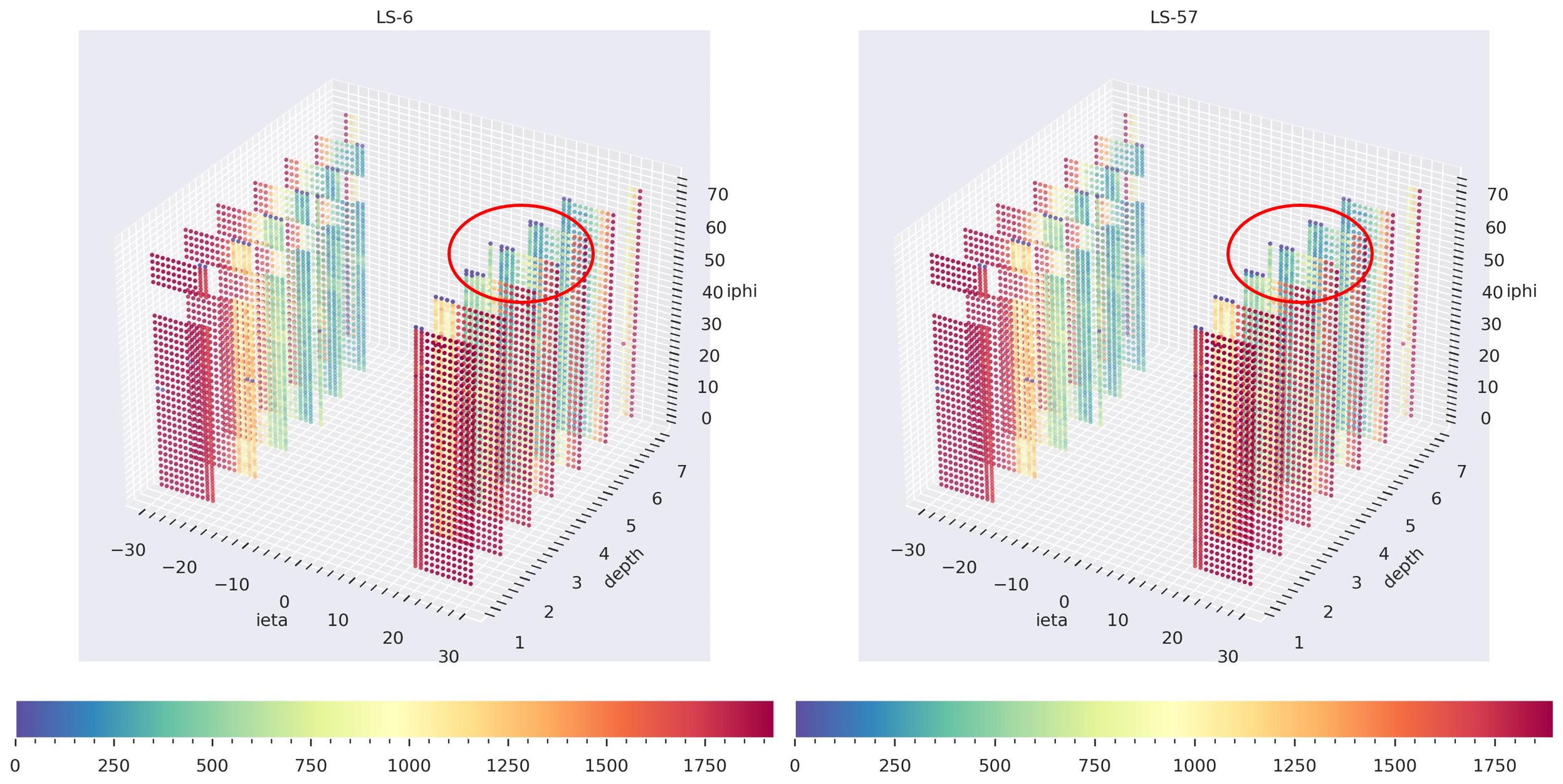
((a))

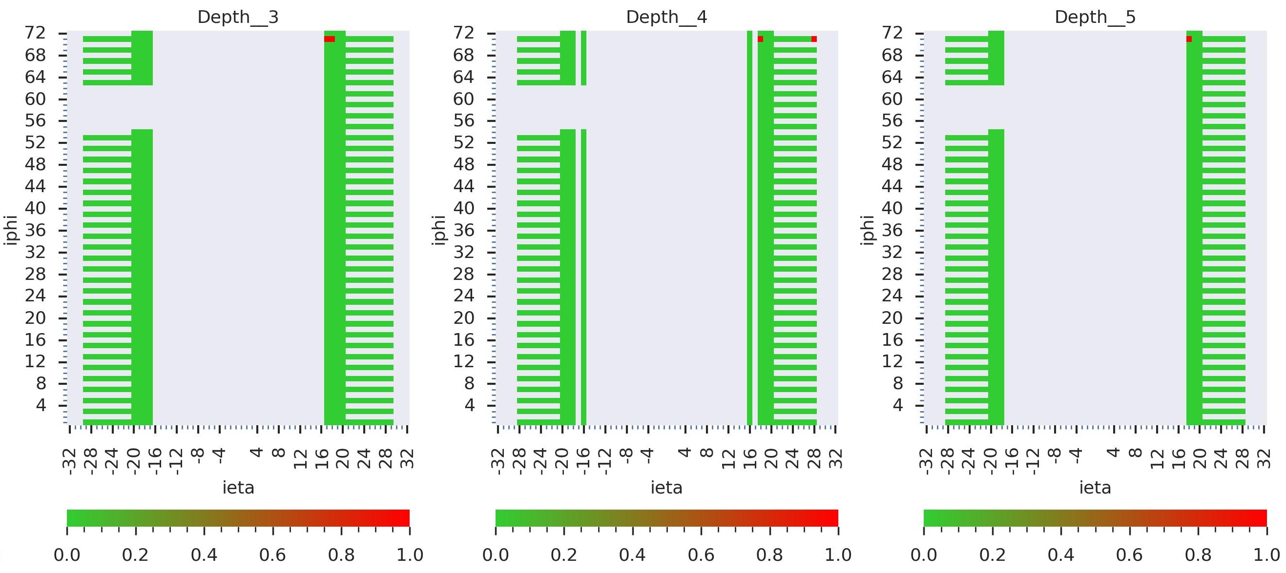
((b))

Figure 13: Detection of real faulty channels from RunId=324841 collision run data. a) the 3D digi-occupancy maps with faulty channels–dead on the left at LS=6 and degraded on the right at LS=57, and b) visualization of the channel anomaly flags on the 2D map per the depth axes–red for anomaly and green for healthy.

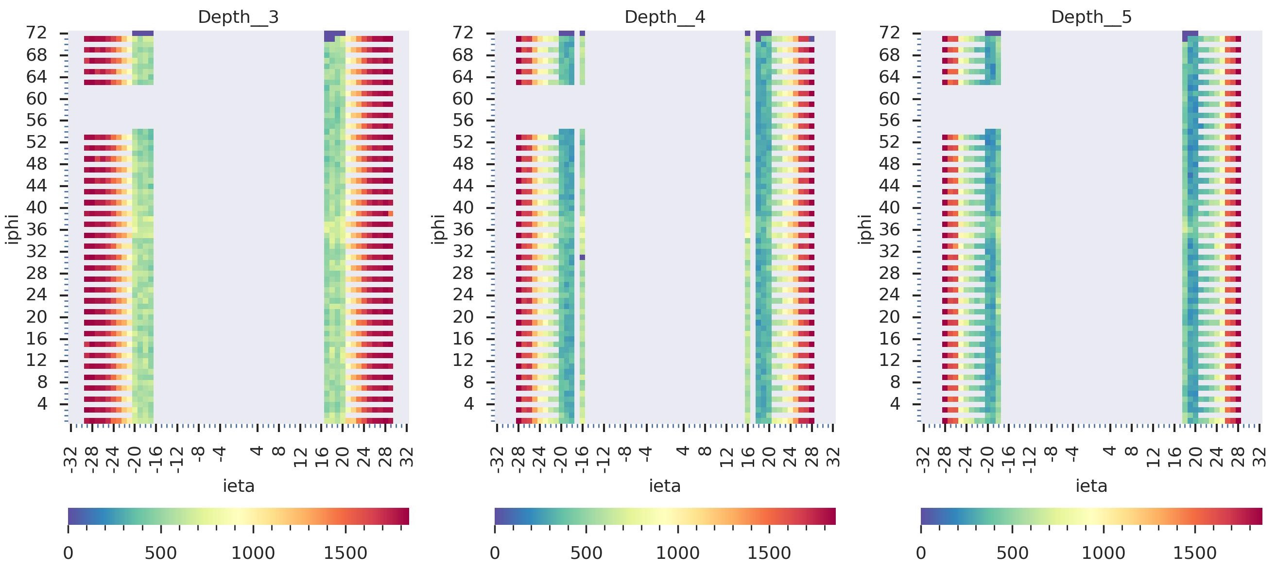
((a))

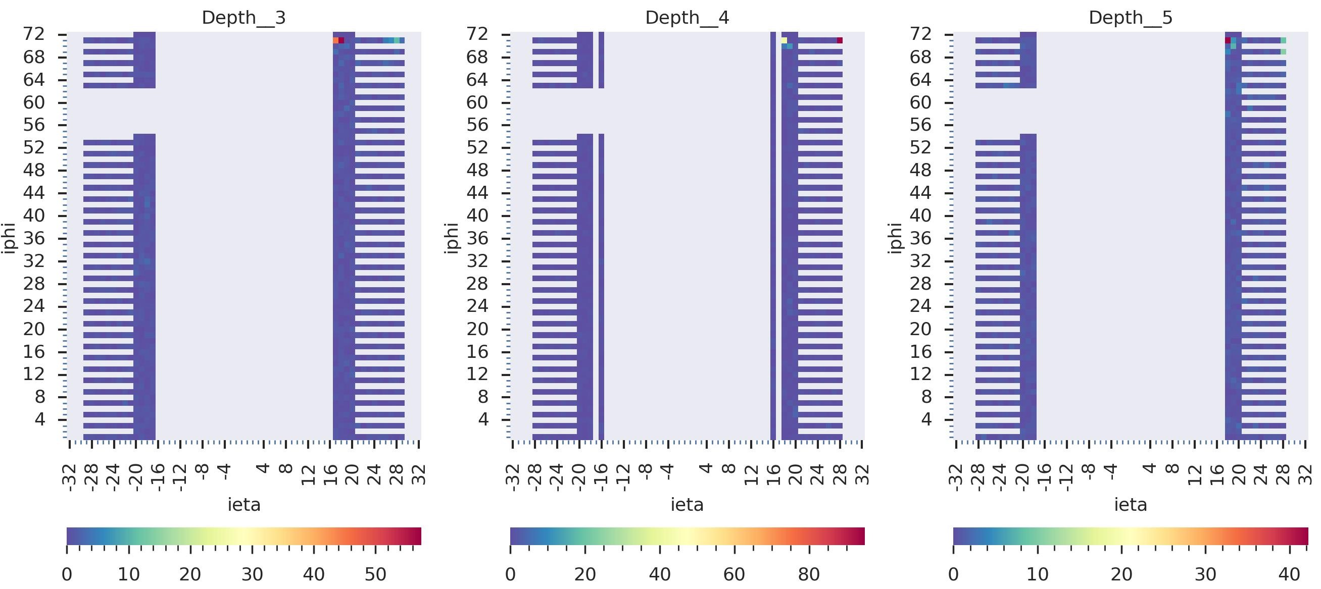
((b))

Figure 14: The detected real dead channels at the LS=6 from the RunId=324841: a) the raw 2D digi-occupancy maps at the depth axes of the faulty channels, and b) the corresponding anomaly score maps. The GraphSTAD localizes the anomaly scores on the faulty dead channels.

((a))

((b))

Figure 15: The detected real degraded channels at the LS=57 from the RunId=324841: a) raw 2D digi-occupancy maps at the depth axes of the faulty channels, and b) the corresponding anomaly visualization maps. The GraphSTAD localizes the anomaly scores on the faulty degraded channels with strength proportional to anomaly severity–lower scores in the color bars than the dead channels.

5.2 Model Computational Cost

We developed the models with PyTorch and trained them on four GPUs of NVIDIA Tesla V100 SXM3 32GB and Intel(R) Xeon(R) Platinum 8168 CPU 2.70GHz. We utilized a time window $T=5$ and batch size $B=8$ for training, and the dimension of a batch is $[B\times T\times N_{i\eta}\times N_{i\phi}\times N_{d}\times N_{f}]$. The training time of the GraphSTAD AE model is approximately 45 seconds per epoch. The training iteration epoch 200 achieves good accuracy with a one-cycle learning rate schedule Smith and Topin (2019). The median inference time of the GraphSTAD on a single GPU is roughly 0.05 seconds with a standard deviation of 0.006 seconds. The integration of the GNN makes the inference relatively slower compared to the benchmark models. The processing cost is, nonetheless, within an acceptable range for the CMS production requirement, as the input digi-occupancy map is generated at each lumisection with a time interval of 23 seconds.

6 Conclusion

Our study presents a semi-supervised anomaly detection system for the hadronic calorimeter’s data quality monitoring system using spatio-temporal digi-occupancy maps. We extend the synergy of temporal deep learning developments for the CMS experiment. Our approach addresses modeling challenges, such as digi-occupancy map renormalization, learning non-Euclidean spatial behavior, and degrading channel detection. To overcome these challenges, we propose the GraphSTAD model, which combines convolutional, graph, and temporal learning networks to capture spatio-temporal behavior and achieve robust localization of anomalies at a channel granularity on high spatial data. The AD performance evaluation has demonstrated the efficacy of the proposed system for channel monitoring. Our proposed AD system will facilitate monitoring and diagnostics of faults in the frontend particle hit sensing hardware and software system of the calorimeter. It will enhance the accuracy and automation of the existing DQM system–providing instant anomaly alerts on a broader range of channel faults in real-time and offline; the improved monitoring of the calorimeter will result in the collection of high-quality physics data. The methods and approaches discussed in this study are domain-agnostic and can be adopted in other spatio-temporal fields–particularly when the data exhibits regular and irregular spatial characteristics.

The CMS-HCAL Collaboration

A. Gevorgyan¹, A. Petrosyan¹, A. Tumasyan¹, G.A. Alves², C. Hensel², W.L. Aldá Júnior³, W. Carvalho³, J. Chinellato^3,f, C. De Oliveira Martins³, D. Matos Figueiredo³, C. Mora Herrera³, H. Nogima³, W.L. Prado Da Silva³, E.J. Tonelli Manganote³, A. Vilela Pereira³, M. Finger⁴, M. Finger Jr.⁴, G. Adamov⁵, Z. Tsamalaidze^5,g, K. Borras^6,y, A. Campbell⁶, F. Engelke^6,y, D. Krücker⁶, I. Martens⁶, L. Wiens^6,y, M. Csanád⁷, A. Feherkuti⁷, S. Lökös^7,v, G. Pásztor⁷, O. Surányi⁷, G.I. Veres⁷, V. Hegde⁸, K. Kothekar⁸, S. Pandey⁸, S. Sharma⁸, S.B. Beri⁹, B. Bhawandeep⁹, R. Chawla⁹, A. Kalsi⁹, A. Kaur⁹, M. Kaur⁹, G. Walia⁹, S. Bhattacharya¹⁰, S. Ghosh¹⁰, S. Nandan¹⁰, A. Purohit¹⁰, M. Sharan¹⁰, S. Banerjee¹¹, S. Bhattacharya¹¹, S. Chatterjee¹¹, P. Das¹¹, M. Guchait¹¹, S. Jain¹¹, S. Kumar¹¹, M. Maity¹¹, G. Majumder¹¹, K. Mazumdar¹¹, M. Patil¹¹, T. Sarkar¹¹ S. Sekmen^12,y, A. Juodagalvis¹³, D. Agyel¹⁴, F. Boran¹⁴, S. Damarseckin¹⁴, Z.S. Demiroglu¹⁴, F. Dölek¹⁴, I. Dumanoglu^14,ee, E. Eskut¹⁴, G. Gokbulut¹⁴, Y. Guler^14,ff, E. Gurpinar Guler^14,ff, C. Işik¹⁴, E.E. Kangal¹⁴, O. Kara¹⁴, A. Kayis Topaksu¹⁴, U. Kiminsu¹⁴, G. Onengut¹⁴, K. Ozdemir^14,gg, E. Pinar¹⁴, A. Polatoz¹⁴, A.E. Simsek¹⁴, B. Tali^14,hh, U.G. Tok¹⁴, S. Turkcapar¹⁴, E. Uslan¹⁴, I.S. Zorbakir¹⁴, B. Bilin^15,y, G. Karapinar^15,ii, A. Murat Guler¹⁵, K. Ocalan^15,jj, M. Yalvac^15,kk, M. Zeyrek¹⁵, B. Akgun¹⁶, I.O. Atakisi^16,ll, E. Gülmez¹⁶, M. Kaya^16,ll, O. Kaya^16,mm, S. Tekten^16,nn, E.A. Yetkin^16,dd, T. Yetkin^16,qq, A. Cakir¹⁷, K. Cankocak^17,ee, S. Sen^17,oo, O. Aydilek¹⁸, S. Cerci^18,hh, B. Hacisahinoglu¹⁸, I. Hos^18,pp, B. Isildak^18,qq, B. Kaynak¹⁸, S. Ozkorucuklu¹⁸, O. Potok¹⁸, H. Sert¹⁸, C. Simsek¹⁸, D. Sunar Cerci^18,hh, C. Zorbilmez¹⁸, A. Boyarintsev¹⁹, B. Grynyov¹⁹, L. Levchuk²⁰, V. Popov²⁰, P. Sorokin²⁰, H. Flacher²¹, S. Abdullin²², B. Caraway²², J. Dittmann²², K. Hatakeyama²², A.R. Kanuganti²², B. McMaster²², M. Saunders²², J. Wilson²², A. Buccilli^23,q, P. Bunin^23,z, S.I. Cooper²³, C. Henderson^23,l, C.U. Perez²³, P. Rumerio^23,t, C. Cosby²⁴, Z. Demiragli²⁴, D. Gastler²⁴, E. Hazen²⁴, J. Rohlf²⁴, M. Hadley²⁵, U. Heintz²⁵, T. Kwon²⁵, E. Laird²⁵, G. Landsberg²⁵, K.T. Lau²⁵, X. Yan²⁵, D. Yu^25,cc, Z. Mao²⁵, J.W. Gary²⁶, G. Karapostoli^26,bb, O.R. Long²⁶, R. Bhandari²⁷, R. Heller²⁷, D. Stuart²⁷, J. Yoo^27,j, Y. Chen^28,n, J. Duarte²⁸, J.M. Lawhorn²⁸, M. Spiropulu²⁸, A. Apresyan²⁹, A. Apyan^29,c, S. Banerjee^29,d, F. Chlebana²⁹, Y. Feng²⁹ J. Freeman²⁹, D. Green²⁹, K.H.M. Kwok²⁹, J. Hirschauer²⁹, U. Joshi²⁹, D. Lincoln²⁹, S. Los²⁹, C. Madrid²⁹, N. Pastika²⁹, K. Pedro²⁹, W.J. Spalding²⁹, S. Tkaczyk²⁹, S. Linn³⁰, P. Markowitz³⁰, V. Hagopian³¹, T. Kolberg³¹, G. Martinez³¹, O. Viazlo³¹, M. Hohlmann³², R. Kumar Verma³², D. Noonan³², F. Yumiceva^32,e, M. Alhusseini³³, B. Bilki³³, D. Blend³³, K. Dilsiz^33,rr, L. Emediato³³, R.P. Gandrajula³³, M. Herrmann³³, O.K. Köseyan³³, J.-P. Merlo³³, A. Mestvirishvili^33,aa, M. Miller³³, H. Ogul^33,ss, Y. Onel³³, A. Penzo³³, D. Southwick³³, E. Tiras^33,tt, J. Wetzel³³, A. Al-bataineh^34,s, J. Bowen^34,o, C. Le Mahieu³⁴, J. Marquez³⁴, W. McBrayer³⁴, M. Murray³⁴, M. Nickel³⁴, S. Popescu^34,r, C. Smith³⁴, Q. Wang³⁴, K. Kaadze³⁵, D. Kim³⁵, Y. Maravin³⁵, A. Mohammadi^35,d, J. Natoli³⁵, D. Roy³⁵, L.K. Saini^35,f, E. Adams³⁶, A. Baden³⁶, O. Baron³⁶, A. Belloni³⁶, A. Bethani³⁶, Y-M Chen³⁶, S.C. Eno³⁶, C. Ferraioli^36,i, T. Grassi³⁶, N.J. Hadley³⁶, R.G. Kellogg³⁶, T. Koeth³⁶, Y. Lai³⁶, S. Lascio³⁶, A.C. Mignerey³⁶, S. Nabili³⁶, C. Palmer³⁶, C. Papageorgakis³⁶, M. Seidel^36,u, L. Wang³⁶, K. Wong³⁶, M. D’Alfonso³⁷, M. Hu³⁷, B. Crossman³⁸, J. Hiltbrand³⁸, M. Krohn³⁸, J. Mans³⁸, M. Revering³⁸, N. Strobbe³⁸, A. Heering³⁹, Y. Musienko^39,z, R. Ruchti³⁹, M. Wayne³⁹, W. Chung⁴⁰, G. Kopp⁴⁰, K. Mei⁴⁰, C. Tully⁴⁰, A. Bodek⁴¹, P. de Barbaro⁴¹, C. Fallon⁴¹, M. Galanti^41,y, A. Garcia-Bellido⁴¹, A. Khukhunaishvili⁴¹, C-L Tan⁴¹, R. Taus⁴¹, D. Vishnevskiy⁴¹, M. Zielinski⁴¹, B. Chiarito⁴², J.P. Chou⁴², S.A. Thayil⁴², H. Wang⁴², N. Akchurin⁴³, J. Damgov⁴³, F. De Guio^43,w, S. Kunori⁴³, K. Lamichhane⁴³, S.W. Lee⁴³, T. Mengke⁴³, S. Muthumuni⁴³, S. Undleeb⁴³, I. Volobouev⁴³, Z. Wang⁴³, A. Whitbeck⁴³, G. Cummings⁴⁴, S. Goadhouse⁴⁴, J. Hakala⁴⁴, R. Hirosky⁴⁴, D. Winn⁴⁵, V. Alexakhin⁴⁶, V. Andreev⁴⁶, Y. Andreev⁴⁶, M. Azarkin⁴⁶, A. Belyaev⁴⁶, S. Bitioukov⁴⁶, E. Boos⁴⁶, O. Bychkova⁴⁶, M. Chadeeva⁴⁶, V. Chekhovsky⁴⁶, R. Chistov⁴⁶, M. Danilov⁴⁶, A. Demianov⁴⁶, A. Dermenev⁴⁶, M. Dubinin^46,k, L. Dudko⁴⁶, D. Elumakhov⁴⁶, V. Epshteyn⁴⁶, Y. Ershov⁴⁶, A. Ershov⁴⁶, V. Gavrilov⁴⁶, I. Golutvin^46,a†, A. Gribushin⁴⁶, A. Kalinin^46,m, A. Kaminskiy⁴⁶, A. Karneyeu⁴⁶, L. Khein⁴⁶, M. Kirakosyan⁴⁶, V. Klyukhin⁴⁶, O. Kodolova^46,b, V. Krychkine⁴⁶, A. Kurenkov⁴⁶, A. Litomin⁴⁶, N. Lychkovskaya⁴⁶, V. Makarenko⁴⁶, P. Mandrik⁴⁶, P. Moisenz^46,a†, S. Obraztsov⁴⁶, A. Oskin⁴⁶, P. Parygin^46,x, V. Petrov⁴⁶, S. Petrushanko⁴⁶, S. Polikarpov⁴⁶, E. Popova^46,x, V. Rusinov⁴⁶, R. Ryutin⁴⁶, V. Savrin⁴⁶, D. Selivanova⁴⁶, V. Smirnov⁴⁶, A. Snigirev⁴⁶, A. Sobol⁴⁶, A. Stepennov^46,p, E. Tarkovskii⁴⁶, A. Terkulov⁴⁶, D. Tlisov^46,a†, I. Tlisova⁴⁶, R. Tolochek⁴⁶, M. Toms^46,h, A. Toropin⁴⁶, S. Troshin⁴⁶, A. Volkov⁴⁶, B. Yuldashev⁴⁶, A. Zarubin⁴⁶, A. Zhokin⁴⁶

¹Yerevan Physics Institute, Yerevan, Armenia
²Centro Brasileiro de Pesquisas Fisicas, Rio de Janeiro, Brazil
³Universidade do Estado do Rio de Janeiro, Rio de Janeiro, Brazil
⁴Charles University, Prague, Czech Republic
⁵Georgian Technical University, Tbilisi, Georgia
⁶Deutsches Elektronen-Synchrotron, Hamburg, Germany
⁷MTA-ELTE Lendület CMS Particle and Nuclear Physics Group, Eötvös Loránd University, Budapest, Hungary
⁸Indian Institute of Science Education and Research (IISER), Pune, India
⁹Panjab University, Chandigarh, India
¹⁰Saha Institute of Nuclear Physics, HBNI, Kolkata, India
¹¹Tata Institute of Fundamental Research-B, Mumbai, India
¹²Kyungpook National University, Daegu, Korea
¹³Vilnius University, Vilnius, Lithuania
¹⁴Çukurova University, Physics Department, Science and Art Faculty, Adana, Turkey
¹⁵Middle East Technical University, Physics Department, Ankara, Turkey
¹⁶Bogazici University, Istanbul, Turkey
¹⁷Istanbul Technical University, Istanbul, Turkey
¹⁸Istanbul University, Istanbul, Turkey
¹⁹Institute for Scintillation Materials of National Academy of Science of Ukraine, Kharkiv, Ukraine
²⁰National Science Centre, Kharkiv Institute of Physics and Technology, Kharkiv, Ukraine
²¹University of Bristol, Bristol, United Kingdom
²²Baylor University, Waco, Texas, USA
²³The University of Alabama, Tuscaloosa, Alabama, USA
²⁴Boston University, Boston, Massachusetts, USA
²⁵Brown University, Providence, Rhode Island, USA
²⁶University of California, Riverside, Riverside, California, USA
²⁷University of California, Santa Barbara - Department of Physics, Santa Barbara, California, USA
²⁸California Institute of Technology, Pasadena, California, USA
²⁹Fermi National Accelerator Laboratory, Batavia, Illinois, USA
³⁰Florida International University, Miami, USA
³¹Florida State University, Tallahassee, Florida, USA
³²Florida Institute of Technology, Melbourne, Florida, USA
³³The University of Iowa, Iowa City, Iowa, USA
³⁴The University of Kansas, Lawrence, Kansas, USA
³⁵Kansas State University, Manhattan, Kansas, USA
³⁶University of Maryland, College Park, Maryland, USA
³⁷Massachusetts Institute of Technology, Cambridge, Massachusetts, USA
³⁸University of Minnesota, Minneapolis, Minnesota, USA
³⁹University of Notre Dame, Notre Dame, Indiana, USA
⁴⁰Princeton University, Princeton, New Jersey, USA
⁴¹University of Rochester, Rochester, New York, USA
⁴²Rutgers, The State University of New Jersey, Piscataway, New Jersey, USA
⁴³Texas Tech University, Lubbock, Texas, USA
⁴⁴University of Virginia, Charlottesville, Virginia, USA
⁴⁵Fairfield University, Fairfield, USA
⁴⁶Authors affiliated with an institute or an international laboratory covered by a cooperation agreement with CERN.

^a†Deceased

^bAlso at Yerevan State University, Yerevan, Armenia

^cNow at Brandeis University, Waltham, USA

^dNow at University of Wisconsin-Madison, Madison, USA

^eNow at Northrop Grumman, Linthicum Heights, USA

^fNow at Gallagher Basset, Schaumburg, USA

^gAlso at Tbilisi State University, Tbilisi, Georgia

^hNow at Karlsruhe Institute of Technology, Karlsruhe, Germany

ⁱNow at Windfall Data, Novato, USA

^jNow at Korea University, Seoul, Korea

^kAlso at California Institute of Technology, Pasadena, California, USA

^lNow at University of Cincinnati, Cincinnati, USA

^mNow at University of Maryland, College Park, Maryland, USA

ⁿNow a Massachusetts Institute of Technology, Cambridge, USA

^oNow at Baker University, Baldwin City, USA

^pNow at University of Cyprus , Cyprus

^qNow at Bond, San Francisco, USA

^rAlso at IFIN-HH, Bucharest, Romania

^sNow at Yarmouk University, Irbid, Jordan

^tAlso at Università di Torino, Torino, Italy

^uNow at Riga Technical University, Riga, Latvia

^vAlso at Karoly Robert Campus, MATE Institute of Technology, Gyongyos, Hungary

^wNow at INFN Sezione di Milano-Bicocca, Milano, Italy

^xNow at University of Rochester, Rochester, New York, USA

^yAlso at CERN, European Organization for Nuclear Research, Geneva, Switzerland

^zAlso at an institute or an international laboratory covered by a cooperation agreement with CERN

^aaAlso at Georgian Technical University, Tbilisi, Georgia

^bbNow at National Technical University of Athens, Greece

^ccNow at University of Nebraska, USA

^ddAlso at Istanbul Bilgi University, Istanbul, Turkey

^eeAlso at Near East University, Research Center of Experimental Health Science, Mersin, Turkey

^ffAlso at Konya Technical University, Konya, Turkey

^ggAlso at Izmir Bakircay University, Izmir, Turkey

^hhAlso at Adiyaman University, Adiyaman, Turkey

ⁱⁱAlso at Istanbul Gedik University, Istanbul, Turkey

^jjAlso at Necmettin Erbakan University, Konya, Turkey

^kkAlso at Bozok Universitetesi Rektörlügü, Yozgat, Turkey

^llAlso at Marmara University, Istanbul, Turkey

^mmAlso at Milli Savunma University, Istanbul, Turkey

ⁿⁿAlso at Kafkas University, Kars, Turkey

^ooAlso at Hacettepe University, Ankara, Turkey

^ppAlso at Istanbul University - Cerrahpasa, Faculty of Engineering, Istanbul, Turkey

^qqAlso at Yildiz Technical University, Istanbul, Turkey

^rrAlso at Bingol University, Bingol, Turkey

^ssAlso at Sinop University, Sinop, Turkey

^ttAlso at Erciyes University, Kayseri, Turkey

References

- Evans and Bryant [2008] Lyndon Evans and Philip Bryant. LHC machine. Journal of instrumentation, 3(08):S08001, 2008.
- Heuer [2012] Rolf-Dieter Heuer. The future of the Large Hadron Collider and CERN. Philosophical Transactions of the Royal Society A: Mathematical, Physical and Engineering Sciences, 370(1961):986–994, 2012.
- Azzolini et al. [2019] Virginia Azzolini, Dmitrijus Bugelskis, Tomas Hreus, Kaori Maeshima, Menendez Javier Fernandez, Antanas Norkus, Patrick James Fraser, Marco Rovere, Marcel Andre Schneider, et al. The data quality monitoring software for the CMS experiment at the lhc: past, present and future. In EPJ Web of Conferences, volume 214, page 02003. EDP Sciences, 2019.
- Tuura et al. [2010] Lassi Tuura, A Meyer, Ilaria Segoni, and G Della Ricca. CMS data quality monitoring: systems and experiences. In Journal of Physics: Conference Series, volume 219, page 072020. IOP Publishing, 2010.
- De Guio and Collaboration [2014] Federico De Guio and The CMS Collaboration. The CMS data quality monitoring software: experience and future prospects. In Journal of Physics: Conference Series, volume 513, page 032024. IOP Publishing, 2014.
- Azzolin et al. [2019] Virginia Azzolin, Michael Andrews, Gianluca Cerminara, Nabarun Dev, Colin Jessop, Nancy Marinelli, Tanmay Mudholkar, Maurizio Pierini, Adrian Pol, and Jean-Roch Vlimant. Improving data quality monitoring via a partnership of technologies and resources between the CMS experiment at CERN and industry. In EPJ Web of Conferences, volume 214, page 01007. EDP Sciences, 2019.
- Pol et al. [2019a] Adrian Alan Pol, Virginia Azzolini, Gianluca Cerminara, Federico De Guio, Giovanni Franzoni, Maurizio Pierini, Filip Sirokỳ, and Jean-Roch Vlimant. Anomaly detection using deep autoencoders for the assessment of the quality of the data acquired by the CMS experiment. In EPJ Web of Conferences, volume 214, page 06008. EDP Sciences, 2019a.
- Pol et al. [2019b] Adrian Alan Pol, Gianluca Cerminara, Cécile Germain, Maurizio Pierini, and Agrima Seth. Detector monitoring with artificial neural networks at the CMS experiment at the CERN Large Hadron Collider. Computing and Software for Big Science, 3(1):3, 2019b.
- Viazlo and Collaboration [2022] Oleksandr Viazlo and The CMS Collaboration. Non-uniformity in HE digi-occupancy distributions. Private communications, 2022.
- Wielgosz et al. [2018] Maciej Wielgosz, Matej Mertik, Andrzej Skoczeń, and Ernesto De Matteis. The model of an anomaly detector for hilumi LHC magnets based on recurrent neural networks and adaptive quantization. Engineering Applications of Artificial Intelligence, 74:166–185, 2018.
- Xu et al. [2017] Dan Xu, Yan Yan, Elisa Ricci, and Nicu Sebe. Detecting anomalous events in videos by learning deep representations of appearance and motion. Computer Vision and Image Understanding, 156:117–127, 2017.
- Chang et al. [2022] Yunpeng Chang, Zhigang Tu, Wei Xie, Bin Luo, Shifu Zhang, Haigang Sui, and Junsong Yuan. Video anomaly detection with spatio-temporal dissociation. Pattern Recognition, 122:108213, 2022.
- Luo et al. [2019] Weixin Luo, Wen Liu, Dongze Lian, Jinhui Tang, Lixin Duan, Xi Peng, and Shenghua Gao. Video anomaly detection with sparse coding inspired deep neural networks. IEEE Transactions on Pattern Analysis and Machine Intelligence, 43(3):1070–1084, 2019.
- Hasan et al. [2016] Mahmudul Hasan, Jonghyun Choi, Jan Neumann, Amit K Roy-Chowdhury, and Larry S Davis. Learning temporal regularity in video sequences. In Proceedings of Computer Vision and Pattern Recognition, pages 733–742. IEEE, 2016.
- Wu et al. [2020] Peng Wu, Jing Liu, Mingming Li, Yujia Sun, and Fang Shen. Fast sparse coding networks for anomaly detection in videos. Pattern Recognition, 107:107515, 2020.
- Hsu [2017] Daniel Hsu. Anomaly detection on graph time series. arXiv preprint arXiv:1708.02975, 2017.
- Ullah et al. [2021] Waseem Ullah, Amin Ullah, Tanveer Hussain, Zulfiqar Ahmad Khan, and Sung Wook Baik. An efficient anomaly recognition framework using an attention residual LSTM in surveillance videos. Sensors, 21(8):2811, 2021.
- Hu et al. [2019] Jingtao Hu, En Zhu, Siqi Wang, Xinwang Liu, Xifeng Guo, and Jianping Yin. An efficient and robust unsupervised anomaly detection method using ensemble random projection in surveillance videos. Sensors, 19(19):4145, 2019.
- Banković et al. [2012] Zorana Banković, David Fraga, José M Moya, and Juan Carlos Vallejo. Detecting unknown attacks in wireless sensor networks that contain mobile nodes. Sensors, 12(8):10834, 2012.
- Zhang et al. [2020] Gangqiang Zhang, Wei Zheng, Wenjie Yin, and Weiwei Lei. Improving the resolution and accuracy of groundwater level anomalies using the machine learning-based fusion model in the North China plain. Sensors, 21(1):46, 2020.
- Atluri et al. [2018] Gowtham Atluri, Anuj Karpatne, and Vipin Kumar. Spatio-temporal data mining: a survey of problems and methods. ACM Computing Surveys, 51(4):1–41, 2018.
- Deng et al. [2022] Leyan Deng, Defu Lian, Zhenya Huang, and Enhong Chen. Graph convolutional adversarial networks for spatiotemporal anomaly detection. IEEE Transactions on Neural Networks and Learning Systems, 33(6):2416–2428, 2022.
- Tišljarić et al. [2021] Leo Tišljarić, Sofia Fernandes, Tonči Carić, and João Gama. Spatiotemporal road traffic anomaly detection: a tensor-based approach. Applied Sciences, 11(24):12017, 2021.
- Jiang et al. [2022] Lin Jiang, Hang Xu, Jinhai Liu, Xiangkai Shen, Senxiang Lu, and Zhan Shi. Anomaly detection of industrial multi-sensor signals based on enhanced spatiotemporal features. Neural Computing and Applications, pages 1–13, 2022.
- Ahmedt-Aristizabal et al. [2021] David Ahmedt-Aristizabal, Mohammad Ali Armin, Simon Denman, Clinton Fookes, and Lars Petersson. Graph-based deep learning for medical diagnosis and analysis: past, present and future. Sensors, 21(14):4758, 2021.
- Duarte and Vlimant [2022] Javier Duarte and Jean-Roch Vlimant. Graph neural networks for particle tracking and reconstruction. In Artificial Intelligence for High Energy Physics, pages 387–436. World Scientific, 2022.
- Shlomi et al. [2020] Jonathan Shlomi, Peter Battaglia, and Jean-Roch Vlimant. Graph neural networks in particle physics. Machine Learning: Science and Technology, 2(2):021001, 2020.
- Qasim et al. [2019] Shah Rukh Qasim, Jan Kieseler, Yutaro Iiyama, and Maurizio Pierini. Learning representations of irregular particle-detector geometry with distance-weighted graph networks. The European Physical Journal C, 79(7):1–11, 2019.
- Martínez et al. [2019] J Arjona Martínez, Olmo Cerri, Maria Spiropulu, JR Vlimant, and M Pierini. Pileup mitigation at the Large Hadron Collider with graph neural networks. The European Physical Journal Plus, 134(7):333, 2019.
- Bruna et al. [2013] Joan Bruna, Wojciech Zaremba, Arthur Szlam, and Yann LeCun. Spectral networks and locally connected networks on graphs. arXiv preprint arXiv:1312.6203, 2013.
- Kipf and Welling [2016] Thomas N Kipf and Max Welling. Semi-supervised classification with graph convolutional networks. arXiv preprint arXiv:1609.02907, 2016.
- Focardi [2012] Ettore Focardi. Status of the CMS detector. Physics Procedia, 37:119–127, 2012.
- Strobbe [2017] Nadja Strobbe. The upgrade of the CMS Hadron Calorimeter with Silicon photomultipliers. Journal of Instrumentation, 12(1):C01080, 2017.
- Rapsevicius et al. [2011] Valdas Rapsevicius, CMS DQM Group, et al. CMS run registry: data certification bookkeeping and publication system. In Journal of Physics: Conference Series, volume 331, page 042038. IOP Publishing, 2011.
- Chalapathy and Chawla [2019] Raghavendra Chalapathy and Sanjay Chawla. Deep learning for anomaly detection: a survey. arXiv preprint arXiv:1901.03407, 2019.
- Kingma and Welling [2013] Diederik P Kingma and Max Welling. Auto-encoding variational bayes. arXiv preprint arXiv:1312.6114, 2013.
- Asres et al. [2021] Mulugeta Weldezgina Asres, Grace Cummings, Pavel Parygin, Aleko Khukhunaishvili, Maria Toms, Alan Campbell, Seth I Cooper, David Yu, Jay Dittmann, and Christian W Omlin. Unsupervised deep variational model for multivariate sensor anomaly detection. In International Conference on Progress in Informatics and Computing, pages 364–371. IEEE, 2021.
- Guo et al. [2018] Yifan Guo, Weixian Liao, Qianlong Wang, Lixing Yu, Tianxi Ji, and Pan Li. Multidimensional time series anomaly detection: A GRU-based gaussian mixture variational autoencoder approach. In Asian Conference on Machine Learning, pages 97–112. Proceedings of Machine Learning Research, 2018.
- An and Cho [2015] Jinwon An and Sungzoon Cho. Variational autoencoder based anomaly detection using reconstruction probability. Special Lecture on IE, 2(1):1–18, 2015.
- Chadha et al. [2019] Gavneet Singh Chadha, Arfyan Rabbani, and Andreas Schwung. Comparison of semi-supervised deep neural networks for anomaly detection in industrial processes. In 17th International Conference on Industrial Informatics, volume 1, pages 214–219. IEEE, 2019.
- Zeiler et al. [2010] Matthew D Zeiler, Dilip Krishnan, Graham W Taylor, and Rob Fergus. Deconvolutional networks. In Proceedings of Computer Vision and Pattern Recognition, pages 2528–2535. IEEE, 2010.
- Smith and Topin [2019] Leslie N Smith and Nicholay Topin. Super-convergence: very fast training of neural networks using large learning rates. In Artificial Intelligence and Machine Learning for Multi-Domain Operations Applications, volume 11006, pages 369–386. SPIE, 2019.