Exact fluctuation and long-range correlations in a single-file model under resetting

Abstract

Resetting is a renewal mechanism in which a process is intermittently repeated after a random or fixed time. This simple act of stop and repeat profoundly influences the behaviour of a system as exemplified by the emergence of non-equilibrium properties and expedition of search processes. Herein, we explore the ramifications of stochastic resetting in the context of a single-file system called random average process (RAP) in one dimension. In particular, we focus on the dynamics of tracer particles and analytically compute the variance, equal time correlation, autocorrelation and unequal time correlation between the positions of different tracer particles. Our study unveils that resetting gives rise to rather different behaviours depending on whether the particles move symmetrically or asymmetrically. For the asymmetric case, the system for instance exhibits a long-range correlation which is not seen in absence of the resetting. Similarly, in contrast to the reset-free RAP, the variance shows distinct scalings for symmetric and asymmetric cases. While for the symmetric case, it decays (towards its steady value) as $\sim e^{-rt}/\sqrt{t}$, we find $\sim te^{-rt}$ decay for the asymmetric case ($r$ being the resetting rate). Finally, we examine the autocorrelation and unequal time correlation in the steady state and demonstrate that they obey interesting scaling forms at late times. All our analytical results are substantiated by extensive numerical simulations.

I INTRODUCTION

Deciphering the behaviour of complex systems consisting of many interacting units is a fundamental problem often encountered in statistical physics [1, 2]. A classic example of an interacting particle system in non-equilibrium statistical mechanics is the single-file system, in which particles in a one-dimensional line move alongside each other, strictly obeying the constraint of non-overtaking, wherein one particle cannot pass another [3, 4, 5]. Due to this non-overtaking constraint (also referred to as single-file constraint), the dynamics of different particles become strongly correlated [6, 7]. For example, in a collection of diffusing particles in one dimension with single-file constraint, the mobility of a tracer particle is drastically reduced and as result, the mean-squared displacement grows sub-diffusively as $\sim\sqrt{t}$ at late times, instead of the linear growth for a freely diffusing particle [8, 9, 10, 11]. The coefficient of this sub-diffusive growth, in turn, depends on the particle number density, the precise interaction among the particles and also on the statistical properties of the initial state of the system [9, 12, 13, 14, 15]. In fact based on hydrodynamic approach, a recent work showed that this sub-diffusive scaling holds true only for short-range interactions and changes to an interaction-dependent exponent for long-range interactions [16]. Beyond diffusion, such slowing down effects have also been studied for Hamiltonian systems [17, 18, 19] as well as for other stochastic systems like randomly accelerated process [20] and active processes [21, 22, 23, 24]. In this paper, we set out to study the tracer dynamics for a single-file model in presence of a renewal mechanism called resetting that has garnered significant attention in the last decade [25].

Stochastic resetting is a simple and natural mechanism in which a dynamical process is intermittently interrupted after some random time, after which it again starts anew. A quintessential example of this phenomenon is the resetting Brownian motion, which was first studied in [25]. In this model, a particle undergoing free diffusion is returned to its starting position at a certain rate $r$, after which it recommences diffusion until the next resetting event. As a result of this, the particle experiences an effective confinement around its initial position. However, it is important to note that this confinement arises solely from the dynamics of the system and does not stem from any physical potential. Indeed, as time progresses, the system eventually reaches a non-equilibrium steady state, which is characterised by the presence of a non-zero probability current. Another notable aspect of this model is that, unlike in free diffusion, the particle exhibits a finite mean first-passage time. Remarkably, this mean time depends non-monotonically on the resetting rate $r$ which indicates its optimisation for an optimal rate $r^{*}$ [26]. Beyond the standard Brownian motion, resetting has also been explored within a broader spectrum of other stochastic processes [27, 28, 29, 30, 31, 32, 33, 34, 35, 36, 37, 38, 39, 40, 41] as well as in cross-disciplinary fields such as search theory [42, 43], computer science [44, 45] and in chemical and biological processes [46, 47, 48, 49]. Furthermore, rigorous studies have been made to comprehend non-Poissonian strategies [50, 29, 51] and the implications of resetting in quantum settings [52, 53, 54, 55, 56]. On the experimental side, resetting was recently realised in experiments involving single particle in optical traps [57, 58, 59, 59]. We refer to [60, 61, 62, 63, 41] and references therein for recent reviews on the subject.

While most of the aforementioned studies primarily focused into single particle dynamics, there has also been a substantial surge of interest in understanding the effects of resetting for interacting particles. Examples include exclusion processes [64, 65, 66, 67], Ising model [68], fluctuating interfaces [69, 70], and predator-prey models [71, 72, 73], among numerous others [see [62] and references therein for a review on stochastic resetting in interacting systems]. These studies investigated the scenario where multiple particles are reset simultaneously after a random duration (global resetting). This is contrary to some other studies where particles reset independently of the other particles (local resetting) [74, 75, 76]. In a recent work involving independently diffusing particles, but undergoing global resetting at a rate $r$, the authors showed that the simultaneous resetting induces a strong long-range correlation in the system [77]. Despite this correlation, the model still possesses analytical solvability based on the renewal formula and many results on the joint probability distribution of the positions and extremal statistics were derived. However, to the best of our knowledge, the implications of stochastic resetting on the dynamics of tracer particles in an interacting multi-particle system still remains unexplored. A natural question that particularly arises - Does one still get a resetting induced long-range correlation in such interacting scenarios? In this paper, we present an example of a single-file model (called random average process) [78, 79] where these questions can be thoroughly addressed through exact analytic computations.

Our system consists of a collection of particles moving in an infinite line and distributed with density $\rho$. We denote the position of $i$-th particle at time $t$ by $x_{i}(t)$ where $i\in\mathbb{Z}$ and $x_{i}(t)\in\mathbb{R}$. Initially, the particles are located at a fixed distance $a=\frac{1}{\rho}$ apart:

$$x_{i}(0)=ia=i/\rho,~{}~{}~{}~{}~{}\text{for all }i\in\mathbb{Z}.$$ (1)

For simplicity, we take $\rho=1$ without any loss of generality. Starting from this configuration, each particle performs the random average process interspersed by resetting events, during which the entire system is (globally) reset to the configuration in Eq. (1). This means that at any small time interval $[t,t+\Delta t]$, two events can occur: (i) either particles globally reset their positions to $x_{i}(0)$ in Eq. (1) with probability $r\Delta t$ (ii) or they perform the random average motion with the remaining probability $(1-r\Delta t)$. In the case of latter event, the $i$-th particle can jump to its right with probability $p\Delta t$ and to its left with probability $q\Delta t$. With remaining probability $\left[1-(p+q)\Delta t\right]$, the position $x_{i}(t)$ does not change. The successful jump, either to the left or to the right, is by a random fraction $\eta_{i}$ of the space available between the particle and its neighbour. This means that the jump to the right takes place by an amount $\eta_{i}\left[x_{i+1}(t)-x_{i}(t)\right]$ while to the left, the particle jumps by the amount $\eta_{i}\left[x_{i-1}(t)-x_{i}(t)\right]$. Here $\eta\in[0,1)$ is a random variable drawn from the distribution $R(\eta)$. Notice that throughout time evolution, a particle can never overtake its neighbouring particles and maintains its initial order.

The overall update rule for the position can then be written as

$$x_{i}(t+\Delta t)=\begin{cases}&x_{i}(0),~{}~{}~{}~{}~{}~{}~{}~{}~{}~{}~{}~{}~{}\text{w.p. }r\Delta t,\\ &x_{i}(t)+\Gamma_{i}(t),~{}~{}~{}~{}\text{w.p. }(1-r\Delta t),\end{cases}$$ (2)

where ‘w.p.’ stands for ‘with probability’ and $\Gamma_{i}(t)$ for the increment which is given by

$$\Gamma_{i}(t)=\begin{cases}&\eta_{i}\left[x_{i+1}(t)-x_{i}(t)\right],~{}~{}\text{w.p. }p\Delta t,\\ &\eta_{i}\left[x_{i-1}(t)-x_{i}(t)\right],~{}~{}\text{w.p. }q\Delta t,\\ &~{}~{}~{}~{}0,~{}~{}~{}~{}~{}~{}~{}~{}~{}~{}~{}~{}~{}~{}~{}~{}~{}~{}~{}~{}~{}\text{w.p. }\left[1-(p+q)\Delta t\right].\end{cases}$$ (3)

Given this model, our aim in this paper is two fold: (i) Firstly, we aim to study the dynamics of tracer particles and explore analytically the effect of stochastic resetting on the single-file model. For this purpose, we investigate the variance and different two-point correlation functions for the positions of tracer particles. In particular, the role of resetting on the autocorrelation involving two different times has so far been studied only for few cases such as the drift-diffusion [38] and the fractional Brownian motion [39]. It also played a crucial role in income dynamics modelled using geometric Brownian motion [80]. However, all of these studies dealt with the single particle dynamics. Here, our aim is to investigate this with multiple particles and understand how fluctuations corresponding to one particle at a given time affect the position of some other particle at some later time. (ii) Secondly, our work will also shed light on determining whether the long-range correlation, stemming from the simultaneous resetting of non-interacting particles [77], persists even when the system involves interacting particles in its underlying dynamics.

The remainder of our paper is organized as follows: Section II briefly recalls the main results of the reset-free random average process. In Section III, we illustrate the effect of resetting on the mean position of a tracer particle. These results will then be used to calculate the variance in Section IV.1 and equal time correlation in Section IV.2. We devote Sections V.1 and V.2 to compute respectively, the autocorrelation and the unequal time correlation in the steady state. Finally, we conclude in Section VI

II Random average process without resetting

Before we delve into discussing the consequences of resetting on tracer particles, it is instructive to review some known results for the random average process (henceforth RAP) in absence of resetting $(r=0)$. Studied originally by Fontes and Ferrari as a generalisation of the smoothing process and the voter model [81], the RAP has appeared in several physical problems like force fluctuations in bead packs [82], in mass transport models [83, 84], in models of wealth distribution and traffic [85] and generalized Hammersley process [86]. As an interacting multi-particle system, this model is particularly interesting since the particles do not overtake each other and maintain their initial order throughout the time evolution as indicated by Eq. (2). Therefore, every particle performs the single-file motion. Due to this non-overtaking constraint, the motion of different particles get strongly correlated [78, 79, 87, 88, 89, 90]. For instance, various studies based on both microscopic calculations as well as hydrodynamic approaches have shown that the variance and the correlation of the displacement variable $z_{i}(t)$ (with $z_{i}(t)=x_{i}(t)-x_{i}(0)$) at late time is given by [79]

$$\langle z_{i}(t)\rangle=\mu_{1}(p-q)t,$$ (4)

$$\langle z_{i}^{2}(t)\rangle-\langle z_{i}(t)\rangle^{2}\simeq\zeta\sqrt{t},$$ (5)

$$\langle z_{0}(t)z_{i}(t)\rangle-\langle z_{i}(t)\rangle\langle z_{0}(t)\rangle$$

$$~{}~{}~{}~{}~{}~{}~{}~{}~{}~{}~{}~{}~{}~{}~{}\simeq\zeta\sqrt{t}~{}f\left(\frac{|i|}{2\sqrt{\mu_{1}(p+q)t}}\right),$$ (6)

where the pre-factor $\zeta=\mu_{2}\sqrt{\mu_{1}(p+q)}/\left[\sqrt{\pi}(\mu_{1}-\mu_{2})\right]$ depends on first two moments $\mu_{1}$ and $\mu_{2}$ of the jump distribution $R(\eta)$ and the scaling function $f(y)$ in Eq. (6) is given by

$$f(y)=e^{-y^{2}}-\sqrt{\pi}y~{}\text{Erfc}(y).$$ (7)

Due to the translational symmetry in the model, both mean and variance in Eqs. (4) and (5) do not depend on the particle index $i$. Also the mean vanishes for the symmetric case $p=q$ since particles do not experience any drive under this condition. Meanwhile the sub-diffusive scaling of the variance at large times in Eq. (5) and the scaling function $f(y)$ in Eq. (7) are hallmark properties of many single-file systems that possess diffusive hydrodynamics at the macroscopic scales [90, 9].

It turns out that the variance and the correlation for single-file systems depend crucially on the statistical properties of the initial state of the system. For RAP, results in Eqs. (4)-(7) hold true only for the quenched initial condition where the initial positions are fixed to Eq. (1) for all realisations [79]. On the other hand, for annealed initial condition where initial positions are drawn from the steady-state, the initial positions themselves vary from realisation to realisation. Under this circumstance, the variance $l_{0}(t)$ at late time grows as

$$l_{0}(t) \simeq\zeta\sqrt{2t},~{}~{}~{}~{}~{}~{}~{}~{}~{}~{}~{}~{}~{}~{}~{}\text{for }p=q,$$ (8)

$$\simeq\frac{\mu_{1}\mu_{2}(p-q)}{(\mu_{1}-\mu_{2})}t,~{}~{}~{}~{}~{}\text{for }p>q.$$ (9)

As indicated, the temporal scaling of $l_{0}(t)$ depends sensitively on whether particles experience drive or not. This is contrary to the quenched case in Eq. (5) where we obtain same scaling for both cases. Furthermore, in the case of symmetric RAP, the ratio of the variances for two cases is found to be $\sqrt{2}$ which is also observed in the context of other single-file models [9, 13]. In what follows, we will investigate these quantities for non-zero $r$ and illustrate how resetting modifies them.

III Average position

For $p\neq q$, we saw in Eq. (4) that the particles experience a net drive which gives rise to a non-zero value of mean that grows linearly with time. Let us investigate what happens to this average in presence of resetting. Here again, it turns out convenient to work in terms of the displacement variable $z_{i}(t)=x_{i}(t)-x_{i}(0)$ and rewrite the update rules in Eq. (2) as

$$z_{i}(t+\Delta t)=\begin{cases}&0,~{}~{}~{}~{}~{}~{}~{}~{}~{}~{}~{}~{}~{}~{}~{}~{}~{}~{}~{}~{}~{}\text{with probability }r\Delta t,\\ &z_{i}(t)+\Gamma_{i}(t),~{}~{}~{}~{}~{}~{}~{}\text{with probability }(1-r\Delta t),\end{cases}$$ (10)

where the increment $\Gamma_{i}(t)$ can be written as

$$\Gamma_{i}(t)=\begin{cases}&\eta_{i}\left[z_{i+1}(t)-z_{i}(t)+1\right],~{}~{}~{}\text{with probability }p\Delta t,\\ &\eta_{i}\left[z_{i-1}(t)-z_{i}(t)-1\right],~{}~{}~{}\text{with probability }q\Delta t,\\ &0,~{}~{}~{}~{}~{}~{}~{}~{}~{}~{}~{}~{}~{}~{}~{}~{}~{}~{}~{}~{}~{}~{}~{}~{}~{}~{}~{}~{}~{}~{}\text{with probability }1-(p+q)\Delta t.\end{cases}$$ (11)

Denoting the mean as $h_{i}(t)=\langle z_{i}(t)\rangle$, we can write its evolution for a small time interval $[t,t+\Delta t]$ as

$$h_{i}(t+\Delta t) \simeq(1-r\Delta t)\left[h_{i}(t)+\langle\Gamma_{i}(t)\rangle\right].$$ (12)

Plugging $\langle\Gamma_{i}(t)\rangle$ from Eq. (11) and taking $\Delta t\to 0$ limit, we obtain the following differential equation for $h_{i}(t)$:

$$\frac{dh_{i}(t)}{dt} =\mu_{1}\left[ph_{i+1}(t)+qh_{i-1}(t)-(p+q)h_{i}(t)\right]$$

$$~{}~{}~{}~{}~{}~{}~{}~{}-rh_{i}(t)+\mu_{1}(p-q).$$ (13)

Recall that $\mu_{m}=\langle\eta^{m}\rangle=\int_{0}^{1}d\eta~{}\eta^{m}R(\eta)$ represents the $m$-th moment of the jump distribution $R(\eta)$. One needs to solve this equation with the initial condition $h_{i}(0)=0$. Since it is a linear equation in $h_{i}(t)$, we proceed to solve it by taking the Fourier transformation with respect to the index $i$. Defining the Fourier transformation as

$$\bar{h}(k,t)=\sum_{i=-\infty}^{\infty}h_{i}(t)~{}e^{jik},$$ (14)

and the inverse Fourier transform as

$$h_{i}(t)=\frac{1}{2\pi}\int_{-\pi}^{\pi}dk~{}\bar{h}(k,t)~{}e^{-jik},$$ (15)

with $j^{2}=-1$, we recast Eq. (13) in terms of the Fourier variable as

$$\frac{\partial\bar{h}(k,t)}{\partial t}=-\alpha(k)~{}\bar{h}(k,t)+2\pi\mu_{1}(p-q)\delta(k),$$ (16)

with $\alpha(k)=r+\mu_{1}(p+q)-\mu_{1}pe^{jk}-\mu_{1}qe^{-jk}$. Finally solving Eq. (16) and performing the inverse Fourier transformation, we get

$$h_{i}(t)=h(t)=\frac{\mu_{1}(p-q)}{r}\left(1-e^{-rt}\right).$$ (17)

Notice that the final expression turns out to be independent of the index $i$, since we have assumed translational invariance of our infinite system. Also, the mean expectedly vanishes for the symmetric $p=q$ case. Meanwhile for $r=0$, our result reduces to Eq. (4) where mean grows linearly with time. However, for any non-zero $r$, it approaches a steady value at large times. This steady value decays as $\sim 1/r$ with respect to the resetting rate. Physically, a larger resetting rate confines the tracer particle to move in the vicinity of its initial position which gives rise to the smaller mean. In Figure 1, we have plotted the mean $h_{i}(t)$ and compared it with the same obtained from numerical simulations. We observe an excellent match between them. In the following sections, we will use this expression of mean to compute different correlation functions for the tracer particles.

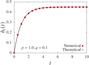
Figure 1: Comparison of the mean $h_{i}(t)=\langle z_{i}(t)\rangle$ in Eq. (17) with the numerical simulation for $p=1.0,~{}q=0.1,~{}r=1$ and jump distribution $R(\eta)=1$. Simulation is conducted with $N=101$ particles.

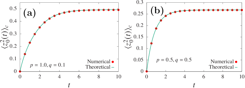
Figure 2: Comparison of $\langle z_{0}^{2}(t)\rangle_{c}$ in Eq. (33) with the numerical simulation for two sets of parameters : $p=1.0,~{}q=0.1$ in panel (a) and $p=0.5,~{}q=0.5$ in panel (b). For both panels, we have performed simulation with $N=101$ particles, resetting rate $r=1$ and jump distribution $R(\eta)=1$.

IV Variance and Equal time correlation

In this section, we look at the variance and equal time correlations of the positions of two tagged particles when the entire system is reset to the configuration in Eq. (1) with rate $r$. Let us denote this correlation by $C_{i}(t)=\langle z_{0}(t)z_{i}(t)\rangle$. Recall that for free RAP, the correlation function satisfies a scaling behaviour in $\big{|}i\big{|}/\sqrt{t}$ with the associated scaling function given in Eq. (7). Here, our aim is to illustrate how this scaling behaviour gets modified in presence of resetting. To this aim, we start by deriving the time evolution differential equation for $C_{i}(t)$. In a small time interval $[t,t+\Delta t]$, the correlation $C_{i}\left(t+\Delta t\right)$ for $i\neq 0$ changes by an amount

$$C_{i}\left(t+\Delta t\right) \simeq C_{i}\left(t\right)-r\Delta t~{}C_{i}\left(t\right)+2\mu_{1}(p-q)\Delta t~{}h(t)$$

$$+\mu_{1}(p+q)\Delta t\left[C_{i+1}(t)+C_{i-1}(t)-2C_{i}(t)\right].$$

On the other hand, applying the same procedure for $i=0$ gives

$$C_{0}\left(t+\Delta t\right) \simeq C_{0}\left(t\right)-r\Delta t~{}C_{0}\left(t\right)+2\mu_{1}(p-q)\Delta t~{}h(t)$$

$$+\mu_{2}(p+q)\Delta t~{}\left[1+2\{C_{0}(t)-C_{1}(t)\}\right]$$

$$+\mu_{1}(p+q)\Delta t\left[2C_{1}(t)-2C_{i}(t)\right]$$

Combining both contributions for $i=0$ and $i\neq 0$ and taking the limit $\Delta t\to 0$, we obtain

$$\frac{dC_{i}(t)}{dt}= \mu_{1}(p+q)\left[C_{i+1}(t)+C_{i-1}(t)-2C_{i}(t)\right]$$

$$+\delta_{i,0}~{}\mu_{2}(p+q)\left[1+2\{C_{0}(t)-C_{1}(t)\}\right]$$

$$~{}~{}~{}~{}~{}+2\mu_{1}(p-q)h(t)-rC_{i}(t).$$ (18)

Fortunately, this equation involves only mean and two-point correlation function and does not involve higher order correlation functions. This closure property enables us to obtain exact solution for this equation. For this, let us take the Laplace transformation with respect to $t~{}(\to s)$ as

$$\hat{C}_{i}(s)=\int_{0}^{\infty}dt~{}e^{-st}~{}C_{i}(t),$$ (19)

and rewrite Eq. (18) in terms of $\hat{C}_{i}(s)$ as

$$s\hat{C}_{i}(s)= ~{}~{}\mu_{1}(p+q)\left[\hat{C}_{i+1}(s)+\hat{C}_{i-1}(s)-2\hat{C}_{i}(s)\right]$$

$$+\delta_{i,0}~{}\mu_{2}(p+q)\left[\frac{1}{s}+2\{\hat{C}_{0}(s)-\hat{C}_{1}(s)\}\right]$$

$$~{}~{}~{}~{}~{}~{}~{}-r\hat{C}_{i}(s)+2\mu_{1}(p-q)\hat{h}(s).$$ (20)

While writing this equation, we have taken the initial condition $C_{i}(0)=0$ and introduced the notation $\hat{h}(s)$ to denote the Laplace transformation of the mean $h(t)$ which from Eq. (17) turns out to be

$$\hat{h}(s)=\frac{\mu_{1}(p-q)}{r}\left(\frac{1}{s}-\frac{1}{s+r}\right).$$ (21)

We now proceed to solve Eq. (20). First notice that, due to the single-file constraint, we get coupling of different $i$ in Eq. (20). To decouple them, we take the Fourier transformation

$$\mathcal{Z}(k,s)=\sum_{i=-\infty}^{\infty}\hat{C}_{i}(s)~{}e^{jik},$$ (22)

and insert this in Eq. (20) to yield

$$\mathcal{Z}(k,s)= \frac{\mu_{2}(p+q)\left[1+2s\{\hat{C}_{0}(s)-\hat{C}_{1}(s)\}\right]}{s\left[s+r+2\mu_{1}(p+q)(1-\cos k)\right]}$$

$$~{}~{}~{}~{}~{}~{}~{}~{}+\frac{4\pi\mu_{1}(p-q)\hat{h}(s)}{(s+r)}~{}\delta(k).$$ (23)

Everything on the right hand side is known except two functions, namely $\hat{C}_{0}(s)$ and $\hat{C}_{1}(s)$. One of them can be expressed in terms of the other by putting $i=0$ in Eq. (20). This results in the relation

$$\hat{C}_{1}(s) =\frac{\left[2(p+q)(\mu_{1}-\mu_{2})+s+r\right]\hat{C}_{0}(s)}{2(\mu_{1}-\mu_{2})(p+q)}$$

$$~{}~{}~{}~{}-\frac{\mu_{2}(p+q)/s+2\mu_{1}(p-q)\hat{h}(s)}{2(\mu_{1}-\mu_{2})(p+q)},$$ (24)

which we substitute in Eq. (23) to yield

$$\mathcal{Z}(k,s)= \frac{\mu_{2}}{s}\frac{\mu_{1}(p+q)-s(s+r)\hat{C}_{0}(s)+2\mu_{1}s(p-q)\hat{h}(s)}{(\mu_{1}-\mu_{2})\left[s+r+2\mu_{1}(p+q)(1-\cos k)\right]}$$

$$~{}~{}~{}~{}~{}~{}~{}~{}+\frac{4\pi\mu_{1}(p-q)\hat{h}(s)}{(s+r)}~{}\delta(k).$$ (25)

We now have only one unknown $\hat{C}_{0}(s)$. However, this can be computed self-consistently as shown later. Finally inverting $\mathcal{Z}(k,s)$ in $k$ gives the exact correlation as

$$\hat{C}_{i}(s)=\frac{2\mu_{1}(p-q)\hat{h}(s)}{s+r}+\hat{\mathcal{G}}_{i}(s),$$ (26)

where the function $\hat{\mathcal{G}}_{i}(s)$ is defined as

$$\hat{\mathcal{G}}_{i}(s) =\frac{\mu_{2}\left[\mu_{1}(p+q)-s(s+r)~{}\hat{\mathcal{G}}_{0}(s)\right]}{s(\mu_{1}-\mu_{2})}\times\mathcal{V}_{i}(s+r),$$ (27)

$$\mathcal{V}_{i}(s) =\frac{1}{2\pi}\int_{-\pi}^{\pi}dk~{}\frac{e^{-jik}}{s+2\mu_{1}^{\prime}(1-\cos k)},$$

$$=\frac{1}{\sqrt{s^{2}+4\mu_{1}^{\prime}s}}\left[\frac{s+2\mu_{1}^{\prime}-\sqrt{s^{2}+4\mu_{1}^{\prime}s}}{2\mu_{1}^{\prime}}\right]^{|i|}$$ (28)

with $\mu_{1}^{\prime}=\mu_{1}(p+q)$. To summarise, we have calculated the exact two-point correlation functions in Eq. (26) in terms of the Laplace variable $s$. The idea now is to perform the inversion and obtain them in the time domain. For simplicity, we carry out this inversion separately for $i=0$ and $i\neq 0$ cases below.

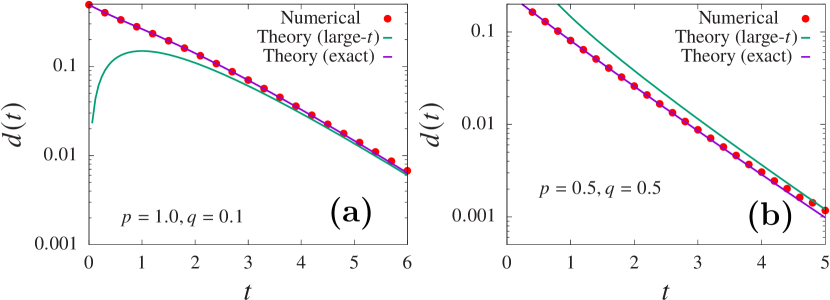
Figure 3: Comparison of the relaxation behaviour of the variance $\langle z_{0}^{2}(t)\rangle_{c}$ for the symmetric $(p=q)$ and asymmetric $(p\neq q)$ cases. For illustration, we have plotted $d(t)=\langle z_{0}^{2}(t\to\infty)\rangle_{c}-\langle z_{0}^{2}(t)\rangle_{c}$ in Eq. (36) and compared it with the numerical simulation for two sets of parameters : $p=1.0~{},q=0.1$ in panel (a) and $p=q=0.5$ in panel (b). For both panels, we have performed simulation with $N=101$ particles, resetting rate $r=1$ and jump distribution $R(\eta)=1$.

IV.1 Variance of $z_{0}(t)$

We first look at the variance for which we put $i=0$ in Eq. (26). Looking at this expression, it is clear that one needs to invert the Laplace transformation $\hat{\mathcal{G}}_{0}(s)$. We rewrite its expression from Eq. (27) as

$$\hat{\mathcal{G}}_{0}(s)=\frac{\mu_{1}\mu_{2}(p+q)(\mu_{1}-\mu_{2})^{-1}(s\sqrt{s+r})^{-1}}{\left[\sqrt{(s+r)+4\mu_{1}(p+q)}+\frac{\mu_{2}}{\mu_{1}-\mu_{2}}\sqrt{s+r}\right]}.$$ (29)

Fortunately, one can perform this inversion exactly and we show in Appendix A that

$$\mathcal{G}_{0}(t)= \frac{\mu_{2}(\mu_{1}-\mu_{2})(p+q)}{\sqrt{r}(\mu_{1}-2\mu_{2})}$$

$$\times\int_{0}^{t}dT~{}e^{-rT}~{}\text{Erf}\left(\sqrt{r(t-T)}\right)~{}Z(T),$$ (30)

where $\mathcal{G}_{0}(t)$ stands for the Laplace transformation of $\hat{\mathcal{G}}_{0}(s)$ and the function $Z(t)$ is defined as

$$Z(t)= \ \frac{1}{\sqrt{\pi t}}\left[e^{-4\mu_{1}t(p+q)}-\frac{\mu_{2}}{\mu_{1}-\mu_{2}}\right]$$

$$-\frac{\mu_{2}}{\mu_{2}-\mu_{2}}~{}\sqrt{-B_{1}}~{}e^{-B_{1}t}~{}\text{Erf}(\sqrt{-B_{1}~{}t})$$ (31)

$$~{}~{}~{}~{}~{}~{}~{}~{}~{}~{}~{}~{}~{}~{}~{}~{}~{}~{}~{}+\sqrt{-B_{2}}~{}e^{-B_{1}t}~{}\text{Erf}(\sqrt{-B_{2}~{}t}).$$

Constants $B_{1}$ and $B_{2}$ depend on the model parameters as $B_{1}=4(p+q)(\mu_{1}-\mu_{2})^{2}/(\mu_{1}-2\mu_{2})$ and $B_{2}=B_{1}-4\mu_{1}(p+q)$. Finally, using Eq. (30) in Eq. (26), we obtain

$$C_{0}(t)=\mathcal{G}_{0}(t)+\frac{2\mu_{1}^{2}(p-q)^{2}}{r^{2}}\left[1-e^{-rt}\left(rt+1\right)\right],$$ (32)

from which the variance of $z_{0}(t)$ turns out to be

$$\langle z_{0}^{2}(t)\rangle_{c} =C_{0}(t)-\langle z_{0}(t)\rangle^{2},$$

$$=\mathcal{G}_{0}(t)+\frac{\mu_{1}^{2}(p-q)^{2}}{r^{2}}\left[1-e^{-rt}\left(2rt+e^{-rt}\right)\right].$$ (33)

This represents the exact variance of the position of a tagged particle in RAP with resetting. Figure 2 illustrates the comparison of our analytical results with the numerical simulations for both symmetric and asymmetric cases. An excellent match is seen in both cases. For any non-zero $r$, we anticipate the expression in Eq. (33) to attain a stationary value at large times. To show this, one can, in principle, directly put $t\to\infty$ in Eq. (30) and carry out the integration. However, it turns out more convenient to put $s\to 0$ limit in $\hat{\mathcal{G}}_{0}(s)$ and use the formula $\mathcal{G}_{0}\left(t\to\infty\right)=\lim_{s\to 0}\left[s\hat{\mathcal{G}}_{0}(s)\right]$. With this procedure, the stationary value of the variance turns out to be

$$\langle z_{0}^{2}(t\to\infty)\rangle_{c}= \frac{\mu_{1}^{2}(p-q)^{2}}{r^{2}}+\frac{\mu_{1}\mu_{2}(p+q)}{\sqrt{r}(\mu_{1}-\mu_{2})}$$

$$\times\left[\sqrt{r+4\mu_{1}(p+q)}+\frac{\mu_{2}\sqrt{r}}{\mu_{1}-\mu_{2}}\right]^{-1}.$$ (34)

Recall that for $r=0$, the tracer particle does not attain any stationary value. This indicates that the stationary value of the variance should diverge as $r\to 0$. From the exact expression in Eq. (34), we find that $\langle z_{0}^{2}(t\to\infty)\rangle_{c}$ diverges differently depending on whether the particles move symmetrically $(p=q)$ or asymmetrically $(p\neq q)$. For $p=q$, the stationary value diverges as $\sim r^{-1/2}$ as $r\to 0$ whereas for $p\neq q$, it diverges as $\sim r^{-2}$. Contrarily for large $r$, $\langle z_{0}^{2}(t\to\infty)\rangle_{c}$ decays as $\sim 1/r$ for both cases.

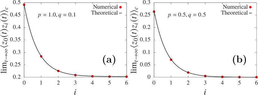
Figure 4: Comparison of the equal time correlation $\langle z_{0}(t)z_{i}(t)\rangle_{c}$ in the steady state $(t\to\infty)$ in Eq. (44) for for two sets of parameters : $p=1.0,~{}q=0.1$ in panel (a) and $p=0.5,~{}q=0.5$ in panel (b). In both panels, simulation has been carried out with $N=101$ particles, resetting rate $r=1$ and jump distribution $R(\eta)=1$.

After analysing the stationary value of the variance, let us look at its time-dependent form in Eq. (33). While this is an exact expression, it has rather a complicated form. To gain some insights in it, we will analyse it for large $t$ and study the relaxation properties. For continuity of presentation, we have shown this calculation in Appendix A and quote only the final result here. We find $d(t)=\langle z_{0}^{2}(t\to\infty)\rangle_{c}-\langle z_{0}^{2}(t)\rangle_{c}$ is given by

$$d(t) \simeq\frac{\mu_{2}\sqrt{\mu_{1}p}}{\sqrt{2\pi}r(\mu_{1}-\mu_{2})}\frac{e^{-rt}}{\sqrt{t}},~{}~{}~{}~{}\text{for }p=q,$$ (35)

$$\simeq\frac{2\mu_{1}^{2}(p-q)^{2}}{r^{2}}rte^{-rt},~{}~{}~{}~{}~{}~{}~{}\text{for }p\neq q.$$ (36)

Interestingly, we find different relaxation behaviours depending on whether $p=q$ or $p\neq q$. While for the symmetric case, the variance relaxes as $\sim e^{-rt}/\sqrt{t}$ to its stationary value, we obtain $\sim te^{-rt}$ relaxation for the asymmetric case. Note that such difference between the symmetric and the asymmetric variances is not seen for free RAP $(r=0)$ and we obtain the same sub-diffusive scaling for both cases as shown in Eq. (5). Indeed, writing the time evolution equation for the variance $\langle z_{0}^{2}(t)\rangle_{c}$ for the free RAP, one can show that it can be made independent of $p$ and $q$ by suitably scaling $t\to(p+q)t$ [79]. Therefore, we get same temporal scaling of the variance for both symmetric and the asymmetric cases. However, in presence of resetting, we get an additional time scale in the problem $\left(\sim 1/r\right)$ and the time evolution equation cannot be rendered independent of $p$ and $q$. This gives rise to different behaviours for two cases. This key difference is one of the consequences of the resetting. In Figure 3, we have compared the relaxation properties with the numerical simulations for $p=q$ case (right panel) and $p\neq q$ case (left panel). We observe an excellent agreement between our theory and numerics for both cases.

IV.2 Correlation $C_{i}(t)=\langle z_{0}(t)z_{i}(t)\rangle$ for $i\neq 0$

After analysing the variance of the position of a tagged particle, let us now look at the position correlation for two different tagged particles. For free RAP, we saw in Eq. (6) that the two-point correlation function satisfies non-trivial scaling behaviour in $\sim|i|/\sqrt{t}$ with $i$ being the separation between two particles. The associated scaling function is given in Eq. (7). In this section, we study the correlation function in presence of resetting and calculate $C_{i}(t)=\langle z_{0}(t)z_{i}(t)\rangle$ for $i\neq 0$. Its expression in the Laplace domain is given in Eq. (26) from which it is clear that we have to perform the inverse Laplace transformation of $\hat{\mathcal{G}}_{i}(s)$. Rewriting its expression from Eq. (27)

$$\hat{\mathcal{G}}_{i}(s)=\hat{\mathcal{G}}_{0}(s)\times\hat{w}_{i}(s+r),$$ (37)

with $$\hat{w}_{i}(s)=\left[\frac{s+2\mu_{1}^{\prime}-\sqrt{s^{2}+4\mu_{1}^{\prime}s}}{2\mu_{1}^{\prime}}\right]^{|i|},$$ (38)

where we have defined $\mu_{1}^{\prime}=\mu_{1}(p+q)$. In order to perform the inverse Laplace transformation of $\hat{\mathcal{G}}_{i}(s)$, we have to carry out two inversions: one is for $\hat{\mathcal{G}}_{0}(s)$ and the other is for $\hat{w}_{i}(s)$. Now for $\hat{\mathcal{G}}_{0}(s)$ , we have already computed this inversion in Eq. (30). On the other hand, for $\hat{w}_{i}(s)$, its inversion in the time domain (denoted by $w_{i}(t)$) is given by [91]

$$w_{i}(t)=\frac{|i|}{t}~{}e^{-2\mu_{1}^{\prime}t}~{}I_{|i|}\left(2\mu_{1}^{\prime}t\right),~{}~{}~{}\text{for }i\neq 0.$$ (39)

Finally using the convolution form of $\hat{\mathcal{G}}_{i}(s)$ in Eq. (37) gives

$$\mathcal{G}_{i}(t)=\int_{0}^{t}dT~{}e^{-rT}~{}w_{i}(T)~{}\mathcal{G}_{0}(t-T).$$ (40)

inserting which in Eq. (26), we obtain

$$C_{i}(t)= \int_{0}^{t}dT~{}e^{-rt}~{}w_{i}(T)~{}\mathcal{G}_{0}(t-T)$$

$$~{}~{}~{}~{}~{}~{}+\frac{2\mu_{1}^{2}(p-q)^{2}}{r^{2}}\left[1-e^{-rt}\left(rt+1\right)\right].$$ (41)

Remember that $C_{i}(t)=\langle z_{0}(t)z_{i}(t)\rangle$ and in order to obtain the connected-correlation, we subtract the mean contributions as follows

$$\langle z_{0}(t)z_{i}(t)\rangle_{c} =\langle z_{0}(t)z_{i}(t)\rangle-\langle z_{0}(t)\rangle\langle z_{i}(t)\rangle,$$

$$=\int_{0}^{t}dT~{}e^{-rt}~{}w_{i}(T)~{}\mathcal{G}_{0}(t-T)$$ (42)

$$~{}~{}~{}~{}~{}+\frac{\mu_{1}^{2}(p-q)^{2}}{r^{2}}\left[1-e^{-rt}\left(2rt+e^{-rt}\right)\right].$$

It is worth mentioning that even for free RAP, only asymptotic results for $\langle z_{0}(t)z_{i}(t)\rangle_{c}$ are known [79]. Our analysis here provides an exact expression for the correlation valid for all times and not just at large times. However, at large times, one can simplify this expression In fact, putting $t\to\infty$ in Eq. (40), one can see that

$$\mathcal{G}_{i}(t\to\infty)=\mathcal{G}_{0}\left(t\to\infty\right)~{}\hat{w}_{i}(r),$$ (43)

where the steady value $\mathcal{G}_{0}\left(t\to\infty\right)$ is given in Eq. (71) and $\hat{w}_{i}(r)$ is given in Eq. (38). Using these expressions, we find that the correlation between two tracer particles in the steady state is given by

$$\langle z_{0}(t)z_{i}(t)\rangle_{c}~{}\stackrel{{\scriptstyle t\to\infty}}{{=}}~{}\mathcal{G}_{0}^{\text{st}}~{}\text{Exp}\left(-\frac{|i|}{\xi_{p}}\right)+\frac{\mu_{1}^{2}(p-q)^{2}}{r^{2}},$$ (44)

where $\mathcal{G}_{0}^{\text{st}}=\mathcal{G}_{0}(t\to\infty)$ is defined in Eq. (71) and the decay length $\xi_{p}$ is defined as

$$\xi_{p}=|\log\left(r+2\mu_{1}^{\prime}-\sqrt{r^{2}+4\mu_{1}^{\prime}r}\right)-\log(2\mu_{1}^{\prime})|^{-1}.$$ (45)

Interestingly for $p\neq q$, we find that the correlation decays to a non-zero constant value as $\big{|}i\big{|}\to\infty$. Contrarily, it decays to zero for $p=q$. For reset-free RAP, this correlation decays to zero both for the symmetric and the asymmetric cases. Our study unravels that resetting affects these two cases in different manners and manifestly gives rise to long-range correlations only for the $p\neq q$ case. Recently, resetting induced long-range correlation was also found in independently diffusing particles but subjected to simultaneous resetting at a rate $r$ [77]. Here, we have extended this result for interacting single-file systems. Physically, the long-range correlation can be understood as follows: Consider two particles with positions $x_{0}(t)$ and $x_{l}(t)$ with $l\gg 1$. Both these particles experience an effective attraction around their initial positions due to the resetting event. However, this attraction has a purely dynamical interpretation and does not arise due to any physical potential. Furthermore, for $p>q$, all particles that lie between $x_{0}(t)$ and $x_{l}(t)$ experience a net drift towards $x_{l}(t)$. As a result of this combined effect of attraction and drift, the positions $x_{0}(t)$ and $x_{l}(t)$ of two particles become strongly correlated. Figure 4 shows the comparison of our analytical results with the same obtained using numerical simulation. Indeed, even in simulations, we find that the correlation $C_{i}(t)$ does not decay to zero for the asymmetric case.

V Unequal time correlations

So far, we have presented rigorous results on the variance and the equal time correlation and demonstrated how resetting modifies these quantities. Our analysis showed that contrary to the reset-free RAP model, these quantities, in presence of resetting, behave differently depending on the presence or absence of drive in the dynamics. Continuing on this, we now look at the autocorrelation and the unequal time position correlations for two tracer particles. Let us denote this correlation by $S_{i}(t_{0},t_{0}+t)=\langle z_{0}(t_{0})z_{i}(t_{0}+t)\rangle$. As done before, we again consider a small time interval $[t_{0}+t,t_{0}+t+dt]$ and follow the update rules in Eqs. (10) and (11) to write down the total change in $S_{i}(t_{0},t_{0}+t)$ within this interval. This results in the following differential equation:

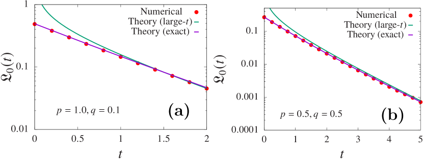
Figure 5: Autocorrelation $\mathcal{L}_{0}(t)$ has been compared with the numerical simulations for $p=1.0,q=0.1$ in panel (a) and $p=0.5,q=0.5$ in panel (b). We have plotted both the exact expression in Eq. (52) as well as the asymptotic (large-$t$) expression in Eq. (54). Simulation has been performed with $N=101$ particles, resetting rate $r=1$ and jump distribution $R(\eta)=1$.

$$\frac{dS_{i}(t_{0},t_{0}+t)}{dt}= -rS_{i}+\mu_{1}(p-q)h(t_{0})$$ (46)

$$+\mu_{1}\Big{[}pS_{i+1}+qS_{i-1}-(p+q)S_{i}\Big{]}.$$

Solving this equation by taking the joint Fourier-Laplace transformations as

$$\tilde{S}(k,t_{0},t_{0}+t)=\sum_{i=-\infty}^{\infty}e^{jik}~{}S_{i}(t_{0},t_{0}+t),$$ (47)

$$\mathbb{S}(k,s,t)=\int_{0}^{\infty}dt_{0}~{}e^{-st_{0}}~{}\tilde{S}(k,t_{0},t_{0}+t),$$ (48)

and inserting them in Eq. (46), we obtain

$$\frac{d\mathbb{S}}{dt}=-\alpha(k)\mathbb{S}+2\pi\mu_{1}(p-q)\hat{h}(s)\delta(k),$$ (49)

where $\alpha(k)=r+\mu_{1}(p+q)-\mu_{1}pe^{jk}-\mu_{1}qe^{-jk}$. Since, we are interested in computing the correlations in the steady state $(\text{i.e. }t_{0}\to\infty)$, we will analyse Eq. (49) in the small-$s$ limit. In Appendix B, we have explicitly carried out this analysis and obtained the correlation $S_{i}\left(t_{0},t_{0}+t\right)$ measured from the steady-state $(t_{0}\to\infty)$ as

$$S_{i}\left(t_{0},t_{0}+t\right) \simeq~{}\frac{\mathcal{B}r}{2\pi}\int_{-\pi}^{\pi}dk~{}\frac{e^{-jik-\alpha(k)t}}{r+2\mu_{1}^{\prime}(1-\cos k)}$$

$$~{}~{}~{}+\frac{\mu_{1}^{2}(p-q)^{2}}{r^{2}}(1+e^{-rt})$$ (50)

$$\text{with }~{}~{}\mathcal{B} =\sqrt{\frac{r+4\mu_{1}^{\prime}}{r}}~{}\mathcal{G}_{0}^{\text{st}},$$ (51)

where again we have used the notation $\mu_{1}^{\prime}=\mu_{1}(p+q)$ and $\mathcal{G}_{0}^{\text{st}}=\mathcal{G}_{0}(t_{0}\to\infty)$ is defined in Eq. (71). Subtracting the mean contribution from this correlation, we obtain the connected-correlation $\mathcal{L}_{i}(t)$ as

$$\mathcal{L}_{i}(t) =\Big{[}S_{i}\left(t_{0},t_{0}+t\right)-\langle z_{0}(t_{0})\rangle~{}\langle z_{i}(t_{0}+t)\rangle\Big{]}_{t_{0}\to\infty},$$

$$=\frac{\mathcal{B}r}{2\pi}\int_{-\pi}^{\pi}dk~{}\frac{e^{-jik-\alpha(k)t}}{r+2\mu_{1}^{\prime}(1-\cos k)}+\frac{\mu_{1}^{2}(p-q)^{2}}{r^{2}}e^{-rt}.$$ (52)

For $t=0$, one can perform the integration over $k$ and the result matches with the equal time correlation in Eq. (44) in the steady state. On the other hand, for non-zero $t$, performing this integration turns out to be difficult. However, for large $t$, we could carry out the integration rigorously and obtain some asymptotic results. Below we discuss this first for the autocorrelation $(i=0)$ and then for general $i$.

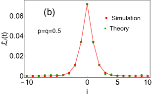
Figure 6: Unequal time correlation $\mathcal{L}_{i}(t)$ in Eq. (52) is compared with the numerical simulation for asymmetric ($p>q$) RAP in the left panel and symmetric ($p=q$) RAP in the right panel for $t=1$. Parameters chosen are $r=1$, $R(\eta)=1$ and number of particles $N=101$ for simulation.

V.1 Autocorrelation $\mathcal{L}_{0}(t)$

To get large $t$-behaviour of $\mathcal{L}_{0}(t)$, we first notice that one gets exponentially decaying terms like $\sim\exp\left[-2\mu_{1}(p+q)t\sin^{2}(k/2)\right]$ inside the integration in Eq. (52). For large $t$, such integrations will be dominated by smaller values of $k$. Therefore, performing small-$k$ approximation in Eq. (52), we get

$$\mathcal{L}_{0}(t)\simeq \frac{\mathcal{B}e^{-rt}}{2\pi}\int_{-\pi}^{\pi}dk~{}e^{jk\mu_{1}(p-q)t-\mu_{1}t(p+q)k^{2}/2}$$

$$~{}~{}~{}~{}~{}~{}~{}~{}~{}~{}~{}~{}~{}~{}~{}~{}~{}+\frac{\mu_{1}^{2}(p-q)^{2}}{r^{2}}e^{-rt}.$$ (53)

Next, we change the variable $u=k\sqrt{\mu_{1}(p+q)t}$ in this equation and carry out the integration for large $t$ to obtain

$$\mathcal{L}_{0}(t)\simeq\frac{\mathcal{B}~{}e^{-\left[r+\frac{\mu_{1}(p-q)^{2}}{2(p+q)}\right]t}}{\sqrt{2\pi\mu_{1}(p+q)t}}+\frac{\mu_{1}^{2}(p-q)^{2}}{r^{2}}e^{-rt}.$$ (54)

Using this expression, we again find that the large time decay of $\mathcal{L}_{0}(t)$ depends on whether the particles experience a drift or not. While for the symmetric case, the autocorrelation in the steady state decays as $\sim e^{-rt}/\sqrt{t}$ at late times, we observe an exponential decay $\sim e^{-rt}$ for the asymmetric $(p\neq q)$ case. This is contrary to the case of simple resetting Brownian motion, where autocorrelation in the steady state decays exponentially as $e^{-rt}$ at all times [38, 39]. However, for interacting particles, $\mathcal{L}_{0}(t)$ has a more complicated form and picks up exponential decay (or otherwise) only at large times. In Figure 5, we have compared this late time decay with the numerical simulations. We observe that while the simulation data deviates from Eq. (54) at small times, the agreement becomes better at larger times.

V.2 Unequal time correlation $\mathcal{L}_{i}(t)$

We now analyse Eq. (52) for general $i$. For this case also, we can perform small-$k$ approximation in Eq. (52) for larger values of $t$ since the integral has exponentially decaying terms like $\sim\exp\left[-2\mu_{1}(p+q)t\sin^{2}(k/2)\right]$. We then obtain

$$\mathcal{L}_{i}(t)\simeq \frac{\mathcal{B}e^{-rt}}{2\pi}\int_{-\pi}^{\pi}dk~{}e^{-jik+jk\mu_{1}(p-q)t-\mu_{1}t(p+q)k^{2}/2}$$

$$~{}~{}~{}~{}~{}~{}~{}~{}~{}~{}~{}~{}~{}~{}~{}~{}~{}+\frac{\mu_{1}^{2}(p-q)^{2}}{r^{2}}e^{-rt}.$$ (55)

To perform the integration over $k$, we change the variable $u=k\sqrt{\mu_{1}(p+q)t}$ and plug it in this equation. Finally, we find that the $\mathcal{L}_{i}(t)$ satisfies the following scaling relation

$$\mathcal{L}_{i}(t)-\mathcal{L}_{|i|\to\infty}(t)\simeq\frac{\mathcal{B}~{}e^{-rt}}{\sqrt{2\pi\mu_{1}(p+q)t}}~{}\mathcal{M}\left(\frac{i-\mu_{1}(p-q)t}{\sqrt{2\mu_{1}(p+q)t}}\right),$$ (56)

where the scaling function $\mathcal{M}(y)$ and $\mathcal{L}_{|i|\to\infty}(t)$ are given by

$$\mathcal{M}(y)=e^{-y^{2}},~{}\text{and }~{}~{}\mathcal{L}_{|i|\to\infty}(t)=\frac{\mu_{1}^{2}(p-q)^{2}}{r^{2}}e^{-rt}.$$ (57)

Note that this scaling behaviour is entirely an outcome of the resetting dynamics and does not appear for the reset-free RAP [79]. Looking at Eq. (56), once again we see that for the asymmetric RAP, $\mathcal{L}_{i}(t)$ takes a non-zero value as $|i|\to\infty$ indicating a long-range correlation between two particles. However, this value decays exponentially with time and as $t\to\infty$, this long-range correlation vanishes. As discussed in the case of equal time correlation, the appearance of long-range correlation turns out to be an interplay of the effective attraction experienced by the particles around their resetting sites and a net drift due to asymmetric rates.

In Figure 6, we have compared the exact expression of $\mathcal{L}_{i}(t)$ in Eq. (52) with the numerical simulations for $p\neq q$ in the left panel and $p=q$ in the right panel. For both cases, we see an excellent agreement between theory and numerics. However, demonstrating the scaling behaviour of $\mathcal{L}_{i}(t)$ in Eq. (56) in simulation turns out to be difficult. It turns out that one needs to go to very large values of $t$ in order to observe this scaling relation. For instance, in Figure 7, we see that this scaling behaviour becomes valid at around $t=200$. However, the value of $\mathcal{L}_{i}(t)$ at such large times is very small due to the presence $\sim e^{-rt}$ term in Eq. (56). Measuring such small values in simulation is difficult. Therefore, to validate this scaling relation, we have plotted the exact $\mathcal{L}_{i}(t)$ in Figure 7 for different values of $t$ by numerically performing the integration over $k$. At large $t$, we recover the scaling function $\mathcal{M}(y)$ [see Figure 7].

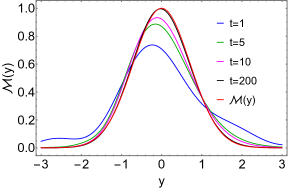
Figure 7: Scaling function $\mathcal{M}(y)$ in Eq. (56) for the unequal time correlation $\mathcal{L}_{i}(t)$ is compared with the exact expression of $\mathcal{L}_{i}(t)$ in Eq. (52) for different values of $t$ and $p=1.0,~{}q=0.1,~{}r=1$ and jump distribution $R(\eta)=1$.

VI Conclusion

In conclusion, we have studied the motion of tracer particles in a one dimensional single-file model called random average process which is subjected to stochastic resetting. The resetting mechanism, characterized by a constant rate $r$ causes the entire system being reinstated to the configuration given in Eq. (1). Utilizing an exact microscopic analysis, we calculated key statistical quantities such as variance, equal-time correlation, autocorrelation, and unequal time correlation for the positions of tracer particles. Through these calculations, we demonstrated how resetting modifies the system and gives rise to properties which are otherwise not observed in absence of the resetting

We first looked at the variance $\langle z_{0}^{2}(t)\rangle_{c}$ whose exact expression is given in Eq. (33). At large times, it expectedly attains a stationary value given in Eq. (34). To gain some physical insights, we further explored the relaxation behaviour of $\langle z_{0}^{2}(t)\rangle_{c}$ as it approaches its stationary value. Interestingly, this relaxation process turns out to crucially depend on whether the particles move symmetrically $(p=q)$ or asymmetrically $(p\neq q)$ on either side. While for the symmetric case, the variance relaxes as $\sim e^{-rt}/\sqrt{t}$ to its stationary value, we obtain $\sim te^{-rt}$ relaxation for the asymmetric case. Note that such difference between the symmetric and the asymmetric variances is not seen for free RAP $(r=0)$ and we obtain the same sub-diffusive scaling for both cases as shown in Eq. (5). Resetting introduces an additional time scale in the model which leads to different behaviours for two cases. This key difference is one of the consequences of the resetting.

We next turned our attention to the equal-time position correlation for two different tracer particles. Focussing on the steady state, our study revealed that resetting induces a long-range correlation only for the asymmetric case. On the other hand, for the symmetric case, we obtained correlations that decay exponentially with the distance in Eq. (44). In a recent work involving independently diffusing particles, but undergoing global resetting at a rate $r$, the authors showed that the simultaneous resetting induces a strong long-range correlation in the system [77]. Our work generalises these results in the interacting single-file set-up and shows that simultaneous resetting induces a long-range correlation only when particles experience a bias $(p\neq q)$.

Finally, we investigated the autocorrelation and the unequal time position correlation in the steady state. For the autocorrelation $\mathcal{L}_{0}(t)$, once again, we find that the large-$t$ decay is different for $p=q$ and $p\neq q$ cases. Specifically, for the symmetric case $\mathcal{L}_{0}(t)$ exhibited a decay of $\sim e^{-rt}/\sqrt{t}$, while for the asymmetric case, the decay followed $\mathcal{L}_{0}(t)\sim e^{-rt}$. Conversely, the unequal time position correlation $\mathcal{L}_{i}(t)$ exhibits a scaling behaviour in terms of the variable $y=\big{(}i-\mu_{1}(p-q)t\big{)}/\sqrt{t}$. The associated scaling function $\mathcal{M}(y)$ is written in Eq. (57). We emphasize that this scaling behaviour is entirely an outcome of the resetting dynamics and does not appear for the reset-free RAP [79].

Studying analytically an interacting multi-particle system is difficult because of the correlation between different particles. Here, we presented a specific single-file model for which exact microscopic computations can be carried out. Our work pointed at a crucial difference in the tracer dynamics for symmetric RAP and asymmetric RAP, both subjected to resetting at a rate $r$. For future direction, it would be interesting to explore an intermediate case where only some of the particles experience bias while all others move symmetrically [87, 88] and see if one still gets a resetting induced long-range correlation. Also, our paper focused on one specific model of single-file motion called random average process. It remains a promising direction to study effects of resetting on other single-file models like single-file diffusion [8, 9, 10, 11], in active particles [92, 93, 94, 21, 22, 23, 24] and also in experiments [57, 58, 59, 59]. Finally, we have only looked at different two-point correlation functions in our paper. Obtaining higher moments and the distribution function for the position of a tracer particle still remains an open problem even for the reset-free RAP.

Appendix A Derivation of the variance $\langle z_{0}^{2}(t)\rangle_{c}$ in Eq. (33)

In this appendix, we provide a detailed derivation of the variance $\langle z_{0}^{2}(t)\rangle_{c}=\langle z_{0}^{2}(t)\rangle-\langle z_{0}(t)\rangle^{2}$ in Eq. (33). The starting point is to find $C_{0}(t)=\langle z_{0}^{2}(t)\rangle$ for which we need the Laplace transform $\hat{C}_{0}(s)$ in Eq. (26). Rewriting this expression here as

$$\hat{C}_{0}(s)=\frac{2\mu_{1}^{2}(p-q)^{2}}{s(s+r)^{2}}+\hat{\mathcal{G}}_{0}(s),$$ (58)

with $\hat{\mathcal{G}}_{0}(s)$ defined as

$$\hat{\mathcal{G}}_{0}(s)=\frac{\mu_{2}(\mu_{1}-\mu_{2})(p+q)}{(\mu_{1}-2\mu_{2})}\hat{H}(s)\hat{Z}(s+r),~{}~{}~{}\text{with }\hat{Z}(s)=\frac{\sqrt{s+4\mu_{1}(p+q)}-\frac{\mu_{2}}{\mu_{1}-\mu_{2}}\sqrt{s}}{s+\frac{4(p+q)(\mu_{1}-\mu_{2})^{2}}{\mu_{1}-2\mu_{2}}},\text{ and }\hat{H}(s)=\frac{1}{s\sqrt{s+r}}.$$ (59)

To evaluate first term in the right hand side of Eq. (58), we use the relation

$$\int_{0}^{\infty}dt~{}e^{-st}\left[\frac{1-e^{-rt}(rt+1)}{r^{2}}\right]=\frac{1}{s(s+r)^{2}}.$$ (60)

On the other hand, for second term, we use the convolution structure of $\hat{\mathcal{G}}_{0}(s)$ which gives $\mathcal{G}_{0}(t)$ as

$$\mathcal{G}_{0}(t)= \frac{\mu_{2}(\mu_{1}-\mu_{2})(p+q)}{(\mu_{1}-2\mu_{2})}\int_{0}^{t}dT~{}e^{-rT}~{}H(t-T)~{}Z(T).$$ (61)

Here $H(t)$ and $Z(t)$ are inverse Laplace transforms of $\hat{H}(s)$ and $\hat{Z}(s)$ respectively. Using Mathematica, we find $H(t)=\text{Erf}\left(\sqrt{rt}\right)/\sqrt{r}$ and $Z(t)$ as

$$Z(t)= \ \frac{1}{\sqrt{\pi t}}\left[e^{-4\mu_{1}t(p+q)}-\frac{\mu_{2}}{\mu_{1}-\mu_{2}}\right]-\frac{\mu_{2}}{\mu_{2}-\mu_{2}}~{}\sqrt{-B_{1}}~{}e^{-B_{1}t}~{}\text{Erf}(\sqrt{-B_{1}~{}t})+\sqrt{-B_{2}}~{}e^{-B_{1}t}~{}\text{Erf}(\sqrt{-B_{2}~{}t}),$$ (62)

with $B_{1}=4(p+q)(\mu_{1}-\mu_{2})^{2}/(\mu_{1}-2\mu_{2})$ and $B_{2}=B_{1}-4\mu_{1}(p+q)$. Substituting these expressions in Eq. (61) yields

$$\mathcal{G}_{0}(t)= \frac{\mu_{2}(\mu_{1}-\mu_{2})(p+q)}{\sqrt{r}(\mu_{1}-2\mu_{2})}\int_{0}^{t}dT~{}e^{-rT}~{}\text{Erf}\left(\sqrt{r(t-T)}\right)~{}Z(T).$$ (63)

We now have both terms from the right hand side of Eq. (58). Performing the inverse Laplace transformation, we get

$$C_{0}(t)=\mathcal{G}_{0}(t)+\frac{2\mu_{1}^{2}(p-q)^{2}}{r^{2}}\left[1-e^{-rt}\left(rt+1\right)\right],$$ (64)

from which the variance of $z_{0}(t)$ turns out to be

$$\langle z_{0}^{2}(t)\rangle_{c} =C_{0}(t)-\langle z_{0}(t)\rangle^{2},$$

$$=\mathcal{G}_{0}(t)+\frac{\mu_{1}^{2}(p-q)^{2}}{r^{2}}\left[1-e^{-rt}\left(2rt+e^{-rt}\right)\right],$$ (65)

with $\mathcal{G}_{0}(t)$ given in Eq. (63). This expression of $\langle z_{0}^{2}(t)\rangle_{c}$ has been quoted in Eq. (33) in the main text.

Let us now analyse this expression to extract the asymptotic behaviour of the variance. To perform the integration in Eq. (63), we substitute the error function for large $t$ as

$$\text{Erf}\left(\sqrt{r(t-T)}\right)\simeq 1-\frac{e^{-r(t-T)}}{\sqrt{\pi r(t-T)}}$$ (66)

and plug it in Eq. (63) as

$$\mathcal{G}_{0}(t)\simeq \frac{\mu_{2}(\mu_{1}-\mu_{2})(p+q)}{\sqrt{r}(\mu_{1}-2\mu_{2})}\left[\int_{0}^{t}dT~{}e^{-rT}Z(T)-\frac{e^{-rt}}{\sqrt{\pi r}}~{}\int_{0}^{t}dT~{}\frac{Z(T)}{\sqrt{t-T}}\right].$$

For $t\to\infty$, first term inside the bracket $[..]$ simply becomes the Laplace transform $\hat{Z}(r)$ in Eq. (59). Therefore, one can recast $\mathcal{G}_{0}(t)$ as

$$\mathcal{G}_{0}(t)\simeq \frac{\mu_{2}(\mu_{1}-\mu_{2})(p+q)}{\sqrt{r}(\mu_{1}-2\mu_{2})}\left[\hat{Z}(r)-\frac{e^{-rt}}{\sqrt{\pi r}}~{}\int_{0}^{t}dT~{}\frac{Z(T)}{\sqrt{t-T}}\right].$$ (67)

Next, we have to evaluate the integral over $T$ for larger values of $t$. Defining $J(t)=\int_{0}^{t}dT~{}\frac{Z(T)}{\sqrt{t-T}}$, we take its Laplace transform with respect to $t~{}(\to s)$ as

$$\hat{J}(s)=\sqrt{\frac{\pi}{s}}~{}\hat{Z}(s).$$ (68)

We take small $s$ limit of this equation which corresponds to its large $t$ limit in the time domain

$$\hat{J}(s\to 0)\simeq\frac{(\mu_{1}-2\mu_{2})\sqrt{\mu_{1}}}{\sqrt{4(p+q)}(\mu_{1}-\mu_{2})^{2}}\sqrt{\frac{\pi}{s}}.$$ (69)

Now performing the inverse Laplace transformation, we obtain

$$J(t)\simeq\frac{(\mu_{1}-2\mu_{2})\sqrt{\mu_{1}}}{\sqrt{4(p+q)t}(\mu_{1}-\mu_{2})^{2}},~{}~{}~{}~{}\text{as }t\to\infty$$ (70)

Using this in Eq. (67), we obtain

$$\mathcal{G}_{0}(t)\simeq \frac{\mu_{1}\mu_{2}(p+q)}{\sqrt{r}(\mu_{1}-\mu_{2})}\left[\sqrt{r+4\mu_{1}(p+q)}+\frac{\mu_{2}\sqrt{r}}{\mu_{1}-\mu_{2}}\right]^{-1}-\frac{\mu_{1}\sqrt{\mu_{1}(p+q)}}{2r(\mu_{1}-\mu_{2})}~{}\frac{e^{-rt}}{\sqrt{\pi t}},$$ (71)

plugging which in Eq. (65) gives the relaxation behaviour of $\langle z_{0}^{2}(t)\rangle_{c}$ in Eqs. (35) and (36).

Appendix B Unequal time correlation $S_{i}\left(t_{0},t_{0}+t\right)$ in the steady state $(t_{0}\to\infty)$

This appendix provides a derivation of the unequal time correlation $S_{i}\left(t_{0},t_{0}+t\right)$ in Eq. (50). Let us first denote by $\mathbb{S}(k,s,t)$ the joint Fourier-Laplace transform of $S_{i}\left(t_{0},t_{0}+t\right)$ [see Eq. (48)]. We showed in Eq. (49) that $\mathbb{S}(k,s,t)$ satisfies the differential equation

$$\frac{d\mathbb{S}(k,s,t)}{dt}=-\alpha(k)\mathbb{S}(k,s,t)+2\pi\mu_{1}(p-q)\hat{h}(s)\delta(k),$$ (72)

where $\alpha(k)=r+\mu_{1}(p+q)-\mu_{1}pe^{jk}-\mu_{1}qe^{-jk}$. Solving this equation with the initial condition $\mathbb{S}(k,s,t=0)=\mathcal{Z}(k,s)$ in Eq. (25) gives

$$\mathbb{S}(k,s,t)=\mathcal{Z}(k,s)~{}e^{-\alpha(k)t}+2\pi\hat{h}(s)h(t).$$ (73)

Since we are interested in finding the correlation at the steady state (i.e. $t_{0}\to\infty$), we analyse Eq. (73) in the small-$s$ limit. For $\hat{h}(s)$, we use Eq. (21) to obtain $\hat{h}(s\to 0)\simeq\mu_{1}(p-q)/rs$. On the other hand, using Eq. (25), we find $\mathcal{Z}(k,s)$ as

$$\mathcal{Z}(k,s\to 0)\simeq\frac{\mathcal{B}r}{s\left[r+2\mu_{1}(p+q)(1-\cos k)\right]}+\frac{4\pi\mu_{1}^{2}(p-q)^{2}}{r^{2}s}~{}\delta(k),$$ (74)

where $\mathcal{B}$ is a constant that depends on model parameters and is given in Eq. (51). Finally plugging Eq. (74) in $\mathbb{S}(k,s,t)$ in Eq. (73) and performing the inverse Fourier transformation, we find

$$S_{i}\left(t_{0},t_{0}+t\right)\Big{|}_{t_{0}\to\infty} =\frac{1}{2\pi}\int_{-\pi}^{\pi}dk~{}e^{-jik}~{}s~{}\mathbb{S}(k,s,t)\Big{|}_{s\to 0},$$ (75)

$$=\frac{\mathcal{B}r}{2\pi}\int_{-\pi}^{\pi}dk~{}\frac{e^{-jik-\alpha(k)t}}{r+2\mu_{1}(p+q)(1-\cos k)}+\frac{\mu_{1}^{2}(p-q)^{2}}{r^{2}}(1+e^{-rt}).$$ (76)

This result has been quoted in Eq. (50) in the main text.

References

- Lieb and Mattis [1966] E. H. Lieb and D. C. Mattis, Mathematical Physics in One Dimension: Exactly Solvable Models of Interacting Particles, 1st ed. (Academic, 1966).
- Privman [1997] V. Privman, Nonequilibrium Statistical Mechanics in One Dimension (Cambridge University Press, 1997).
- Harris [1965] T. E. Harris, Diffusion with collisions between particles, Journal of Applied Probability 2, 323–338 (1965).
- Jepsen [2004] D. W. Jepsen, Dynamics of a Simple Many‐Body System of Hard Rods, Journal of Mathematical Physics 6, 405 (2004).
- Arratia [1983] R. Arratia, The Motion of a Tagged Particle in the Simple Symmetric Exclusion System on , The Annals of Probability 11, 362 (1983).
- Poncet et al. [2021] A. Poncet, A. Grabsch, P. Illien, and O. Bénichou, Generalized correlation profiles in single-file systems, Phys. Rev. Lett. 127, 220601 (2021).
- Grabsch et al. [2023] A. Grabsch, P. Rizkallah, A. Poncet, P. Illien, and O. Bénichou, Exact spatial correlations in single-file diffusion, Phys. Rev. E 107, 044131 (2023).
- Krapivsky et al. [2015a] P. L. Krapivsky, K. Mallick, and T. Sadhu, Dynamical properties of single-file diffusion, Journal of Statistical Mechanics: Theory and Experiment 2015, P09007 (2015a).
- Krapivsky et al. [2014] P. L. Krapivsky, K. Mallick, and T. Sadhu, Large deviations in single-file diffusion, Phys. Rev. Lett. 113, 078101 (2014).
- Bénichou et al. [2018] O. Bénichou, P. Illien, G. Oshanin, A. Sarracino, and R. Voituriez, Tracer diffusion in crowded narrow channels, Journal of Physics: Condensed Matter 30, 443001 (2018).
- Alexander and Pincus [1978] S. Alexander and P. Pincus, Diffusion of labeled particles on one-dimensional chains, Phys. Rev. B 18, 2011 (1978).
- Krapivsky et al. [2015b] P. L. Krapivsky, K. Mallick, and T. Sadhu, Tagged particle in single-file diffusion, Journal of Statistical Physics 160, 885–925 (2015b).
- Banerjee et al. [2022a] T. Banerjee, R. L. Jack, and M. E. Cates, Role of initial conditions in one-dimensional diffusive systems: Compressibility, hyperuniformity, and long-term memory, Phys. Rev. E 106, L062101 (2022a).
- Barkai and Silbey [2009] E. Barkai and R. Silbey, Theory of single file diffusion in a force field, Phys. Rev. Lett. 102, 050602 (2009).
- Leibovich and Barkai [2013] N. Leibovich and E. Barkai, Everlasting effect of initial conditions on single-file diffusion, Phys. Rev. E 88, 032107 (2013).
- Dandekar et al. [2023] R. Dandekar, P. L. Krapivsky, and K. Mallick, Dynamical fluctuations in the riesz gas, Phys. Rev. E 107, 044129 (2023).
- Hegde et al. [2014] C. Hegde, S. Sabhapandit, and A. Dhar, Universal large deviations for the tagged particle in single-file motion, Phys. Rev. Lett. 113, 120601 (2014).
- Roy et al. [2013] A. Roy, O. Narayan, A. Dhar, and S. Sabhapandit, Tagged particle diffusion in one-dimensional gas with hamiltonian dynamics, Journal of Statistical Physics 150, 851–866 (2013).
- Kollmann [2003] M. Kollmann, Single-file diffusion of atomic and colloidal systems: Asymptotic laws, Phys. Rev. Lett. 90, 180602 (2003).
- Burkhardt [2019] T. W. Burkhardt, Tagged-particle statistics in single-file motion with random-acceleration and langevin dynamics, Journal of Statistical Physics 177, 806–824 (2019).
- Teomy and Metzler [2019] E. Teomy and R. Metzler, Transport in exclusion processes with one-step memory: density dependence and optimal acceleration, Journal of Physics A: Mathematical and Theoretical 52, 385001 (2019).
- Galanti et al. [2013] M. Galanti, D. Fanelli, and F. Piazza, Persistent random walk with exclusion, Eur. Phys. J. B 456, 86 (2013).
- Dolai et al. [2020] P. Dolai, A. Das, A. Kundu, C. Dasgupta, A. Dhar, and K. V. Kumar, Universal scaling in active single-file dynamics, Soft Matter 16, 7077 (2020).
- Banerjee et al. [2022b] T. Banerjee, R. L. Jack, and M. E. Cates, Tracer dynamics in one dimensional gases of active or passive particles, Journal of Statistical Mechanics: Theory and Experiment 2022, 013209 (2022b).
- Evans and Majumdar [2011a] M. R. Evans and S. N. Majumdar, Diffusion with stochastic resetting, Phys. Rev. Lett. 106, 160601 (2011a).
- Evans and Majumdar [2011b] M. R. Evans and S. N. Majumdar, Diffusion with optimal resetting, Journal of Physics A: Mathematical and Theoretical 44, 435001 (2011b).
- Majumdar et al. [2015] S. N. Majumdar, S. Sabhapandit, and G. Schehr, Dynamical transition in the temporal relaxation of stochastic processes under resetting, Phys. Rev. E 91, 052131 (2015).
- Pal [2015] A. Pal, Diffusion in a potential landscape with stochastic resetting, Phys. Rev. E 91, 012113 (2015).
- Pal and Reuveni [2017] A. Pal and S. Reuveni, First passage under restart, Phys. Rev. Lett. 118, 030603 (2017).
- Kusmierz et al. [2014] L. Kusmierz, S. N. Majumdar, S. Sabhapandit, and G. Schehr, First order transition for the optimal search time of lévy flights with resetting, Phys. Rev. Lett. 113, 220602 (2014).
- Bressloff [2020a] P. C. Bressloff, Directed intermittent search with stochastic resetting, Journal of Physics A: Mathematical and Theoretical 53, 105001 (2020a).
- Reuveni [2016] S. Reuveni, Optimal stochastic restart renders fluctuations in first passage times universal, Phys. Rev. Lett. 116, 170601 (2016).
- Gupta [2019] D. Gupta, Stochastic resetting in underdamped brownian motion, Journal of Statistical Mechanics: Theory and Experiment 2019, 033212 (2019).
- Singh [2020] P. Singh, Random acceleration process under stochastic resetting, Journal of Physics A: Mathematical and Theoretical 53, 405005 (2020).
- Evans and Majumdar [2018] M. R. Evans and S. N. Majumdar, Run and tumble particle under resetting: a renewal approach, Journal of Physics A: Mathematical and Theoretical 51, 475003 (2018).
- Kumar et al. [2020] V. Kumar, O. Sadekar, and U. Basu, Active brownian motion in two dimensions under stochastic resetting, Phys. Rev. E 102, 052129 (2020).
- Singh and Pal [2021] P. Singh and A. Pal, Extremal statistics for stochastic resetting systems, Phys. Rev. E 103, 052119 (2021).
- Stojkoski et al. [2022a] V. Stojkoski, T. Sandev, L. Kocarev, and A. Pal, Autocorrelation functions and ergodicity in diffusion with stochastic resetting, Journal of Physics A: Mathematical and Theoretical 55, 104003 (2022a).
- Majumdar and Oshanin [2018] S. N. Majumdar and G. Oshanin, Spectral content of fractional brownian motion with stochastic reset, Journal of Physics A: Mathematical and Theoretical 51, 435001 (2018).
- Singh and Pal [2022] P. Singh and A. Pal, First-passage brownian functionals with stochastic resetting, Journal of Physics A: Mathematical and Theoretical 55, 234001 (2022).
- Pal et al. [2022] A. Pal, S. Kostinski, and S. Reuveni, The inspection paradox in stochastic resetting, Journal of Physics A: Mathematical and Theoretical 55, 021001 (2022).
- Pal et al. [2020] A. Pal, L. Kuśmierz, and S. Reuveni, Search with home returns provides advantage under high uncertainty, Phys. Rev. Res. 2, 043174 (2020).
- Montanari and Zecchina [2002] A. Montanari and R. Zecchina, Optimizing searches via rare events, Phys. Rev. Lett. 88, 178701 (2002).
- Luby et al. [1993] M. Luby, A. Sinclair, and D. Zuckerman, Optimal speedup of las vegas algorithms, Information Processing Letters 47, 173 (1993).
- Hamlin et al. [2019] P. Hamlin, W. J. Thrasher, W. Keyrouz, and M. Mascagni, Geometry entrapment in walk-on-subdomains, Monte Carlo Methods and Applications 25, 329 (2019).
- Reuveni et al. [2014] S. Reuveni, M. Urbakh, and J. Klafter, Role of substrate unbinding in michaelis–menten enzymatic reactions, Proceedings of the National Academy of Sciences 111, 4391 (2014), https://www.pnas.org/doi/pdf/10.1073/pnas.1318122111 .
- Roldán et al. [2016] E. Roldán, A. Lisica, D. Sánchez-Taltavull, and S. W. Grill, Stochastic resetting in backtrack recovery by rna polymerases, Phys. Rev. E 93, 062411 (2016).
- Bressloff [2020b] P. C. Bressloff, Modeling active cellular transport as a directed search process with stochastic resetting and delays, Journal of Physics A: Mathematical and Theoretical 53, 355001 (2020b).
- Pal et al. [2021] A. Pal, S. Reuveni, and S. Rahav, Thermodynamic uncertainty relation for first-passage times on markov chains, Phys. Rev. Res. 3, L032034 (2021).
- Nagar and Gupta [2016] A. Nagar and S. Gupta, Diffusion with stochastic resetting at power-law times, Phys. Rev. E 93, 060102 (2016).
- Chechkin and Sokolov [2018] A. Chechkin and I. M. Sokolov, Random search with resetting: A unified renewal approach, Phys. Rev. Lett. 121, 050601 (2018).
- Mukherjee et al. [2018] B. Mukherjee, K. Sengupta, and S. N. Majumdar, Quantum dynamics with stochastic reset, Phys. Rev. B 98, 104309 (2018).
- Kulkarni and Majumdar [2023] M. Kulkarni and S. N. Majumdar, Generating entanglement by quantum resetting, https://arxiv.org/abs/2307.07485 (2023), arXiv:2307.07485.
- Yin and Barkai [2023a] R. Yin and E. Barkai, Restart expedites quantum walk hitting times, Phys. Rev. Lett. 130, 050802 (2023a).
- Yin and Barkai [2023b] R. Yin and E. Barkai, Instability in the quantum restart problem, https://arxiv.org/abs/2301.06100 (2023b), arXiv:2301.06100.
- Dubey et al. [2023] V. Dubey, R. Chetrite, and A. Dhar, Quantum resetting in continuous measurement induced dynamics of a qubit, Journal of Physics A: Mathematical and Theoretical 56, 154001 (2023).
- Tal-Friedman et al. [2020] O. Tal-Friedman, A. Pal, A. Sekhon, S. Reuveni, and Y. Roichman, Experimental realization of diffusion with stochastic resetting, The Journal of Physical Chemistry Letters 11, 7350 (2020), pMID: 32787296, https://doi.org/10.1021/acs.jpclett.0c02122 .
- Besga et al. [2020] B. Besga, A. Bovon, A. Petrosyan, S. N. Majumdar, and S. Ciliberto, Optimal mean first-passage time for a brownian searcher subjected to resetting: Experimental and theoretical results, Phys. Rev. Res. 2, 032029 (2020).
- Besga et al. [2021] B. Besga, F. Faisant, A. Petrosyan, S. Ciliberto, and S. N. Majumdar, Dynamical phase transition in the first-passage probability of a brownian motion, Phys. Rev. E 104, L012102 (2021).
- Evans et al. [2020] M. R. Evans, S. N. Majumdar, and G. Schehr, Stochastic resetting and applications, Journal of Physics A: Mathematical and Theoretical 53, 193001 (2020).
- Gupta and Jayannavar [2022] S. Gupta and A. M. Jayannavar, Stochastic resetting: A (very) brief review, Frontiers in Physics 10, 10.3389/fphy.2022.789097 (2022).
- Nagar and Gupta [2023] A. Nagar and S. Gupta, Stochastic resetting in interacting particle systems: a review, Journal of Physics A: Mathematical and Theoretical 56, 283001 (2023).
- Pal et al. [2023] A. Pal, V. Stojkoski, and T. Sandev, Random resetting in search problems, https://arxiv.org/abs/2310.12057 (2023), arXiv:2310.12057.
- Basu et al. [2019] U. Basu, A. Kundu, and A. Pal, Symmetric exclusion process under stochastic resetting, Phys. Rev. E 100, 032136 (2019).
- Sadekar and Basu [2020] O. Sadekar and U. Basu, Zero-current nonequilibrium state in symmetric exclusion process with dichotomous stochastic resetting, Journal of Statistical Mechanics: Theory and Experiment 2020, 073209 (2020).
- Karthika and Nagar [2020] S. Karthika and A. Nagar, Totally asymmetric simple exclusion process with resetting, Journal of Physics A: Mathematical and Theoretical 53, 115003 (2020).
- Mishra and Basu [2023] S. Mishra and U. Basu, Symmetric exclusion process under stochastic power-law resetting, Journal of Statistical Mechanics: Theory and Experiment 2023, 053202 (2023).
- Magoni et al. [2020] M. Magoni, S. N. Majumdar, and G. Schehr, Ising model with stochastic resetting, Phys. Rev. Res. 2, 033182 (2020).
- Gupta et al. [2014] S. Gupta, S. N. Majumdar, and G. Schehr, Fluctuating interfaces subject to stochastic resetting, Phys. Rev. Lett. 112, 220601 (2014).
- Gupta and Nagar [2016] S. Gupta and A. Nagar, Resetting of fluctuating interfaces at power-law times, Journal of Physics A: Mathematical and Theoretical 49, 445001 (2016).
- Mercado-Vásquez and Boyer [2018] G. Mercado-Vásquez and D. Boyer, Lotka–volterra systems with stochastic resetting, Journal of Physics A: Mathematical and Theoretical 51, 405601 (2018).
- Evans et al. [2022] M. R. Evans, S. N. Majumdar, and G. Schehr, An exactly solvable predator prey model with resetting, Journal of Physics A: Mathematical and Theoretical 55, 274005 (2022).
- Singh and Singh [2022] R. K. Singh and S. Singh, Capture of a diffusing lamb by a diffusing lion when both return home, Phys. Rev. E 106, 064118 (2022).
- Krapivsky et al. [2022] P. L. Krapivsky, O. Vilk, and B. Meerson, Competition in a system of brownian particles: Encouraging achievers, Phys. Rev. E 106, 034125 (2022).
- Miron and Reuveni [2021] A. Miron and S. Reuveni, Diffusion with local resetting and exclusion, Phys. Rev. Res. 3, L012023 (2021).
- Pelizzola et al. [2021] A. Pelizzola, M. Pretti, and M. Zamparo, Simple exclusion processes with local resetting, Europhysics Letters 133, 60003 (2021).
- Biroli et al. [2023] M. Biroli, H. Larralde, S. N. Majumdar, and G. Schehr, Extreme statistics and spacing distribution in a brownian gas correlated by resetting, Phys. Rev. Lett. 130, 207101 (2023).
- Schütz [2000] G. M. Schütz, Exact tracer diffusion coefficient in the asymmetric random average process, Journal of Statistical Physics 99, 1045 (2000).
- Rajesh and Majumdar [2001] R. Rajesh and S. N. Majumdar, Exact tagged particle correlations in the random average process, Phys. Rev. E 64, 036103 (2001).
- Stojkoski et al. [2022b] V. Stojkoski, P. Jolakoski, A. Pal, T. Sandev, L. Kocarev, and R. Metzler, Income inequality and mobility in geometric brownian motion with stochastic resetting: theoretical results and empirical evidence of non-ergodicity, Philosophical Transactions of the Royal Society A: Mathematical, Physical and Engineering Sciences 380, 20210157 (2022b).
- Ferrari and Fontes [1998] P. Ferrari and L. Fontes, Fluctuations of a Surface Submitted to a Random Average Process, Electronic Journal of Probability 3, 1 (1998).
- Coppersmith et al. [1996] S. N. Coppersmith, C. h. Liu, S. Majumdar, O. Narayan, and T. A. Witten, Model for force fluctuations in bead packs, Phys. Rev. E 53, 4673 (1996).
- Rajesh and Majumdar [2000] R. Rajesh and S. N. Majumdar, Conserved mass models and particle systems in one dimension, Journal of Statistical Physics 99, 943–965 (2000).
- Krug and Garcia [2000] J. Krug and J. Garcia, Asymmetric particle systems on r, Journal of Statistical Physics 99, 31–55 (2000).
- Ispolatov et al. [1998] S. Ispolatov, P. L. Krapivsky, and S. Redner, Wealth distributions in asset exchange models, The European Physical Journal B - Condensed Matter and Complex Systems 2, 267 (1998).
- Aldous and Diaconis [1995] D. Aldous and P. Diaconis, Hammersley’s interacting particle process and longest increasing subsequences, Probability Theory and Related Fields 103, 199 (1995).
- Cividini et al. [2016a] J. Cividini, A. Kundu, S. N. Majumdar, and D. Mukamel, Exact gap statistics for the random average process on a ring with a tracer, Journal of Physics A: Mathematical and Theoretical 49, 085002 (2016a).
- Kundu and Cividini [2016] A. Kundu and J. Cividini, Exact correlations in a single-file system with a driven tracer, Europhysics Letters 115, 54003 (2016).
- Cividini et al. [2016b] J. Cividini, A. Kundu, S. N. Majumdar, and D. Mukamel, Correlation and fluctuation in a random average process on an infinite line with a driven tracer, Journal of Statistical Mechanics: Theory and Experiment 2016, 053212 (2016b).
- Cividini and Kundu [2017] J. Cividini and A. Kundu, Tagged particle in single-file diffusion with arbitrary initial conditions, Journal of Statistical Mechanics: Theory and Experiment 2017, 083203 (2017).
- Bateman and Project [2023] H. Bateman and B. M. Project, Tables of Integral Transforms (McGraw-Hill Book Company, 2023).
- Singh and Kundu [2021] P. Singh and A. Kundu, Crossover behaviours exhibited by fluctuations and correlations in a chain of active particles, Journal of Physics A: Mathematical and Theoretical 54, 305001 (2021).
- Put et al. [2019] S. Put, J. Berx, and C. Vanderzande, Non-gaussian anomalous dynamics in systems of interacting run-and-tumble particles, Journal of Statistical Mechanics: Theory and Experiment 2019, 123205 (2019).
- Santra et al. [2023] S. Santra, P. Singh, and A. Kundu, Tracer dynamics in active random average process, https://arxiv.org/abs/2307.09908 (2023), arXiv:2307.09908.