Enhanced power spectra from multi-field inflation

Abstract

We investigate the enhancement of the power spectra in models with multiple scalar fields large enough to produce primordial black holes. We derive the criteria that can lead to an exponential amplification of the curvature perturbation on subhorizon scales, while leaving the perturbations stable on superhorizon scales. We apply our results on the three-field ultra-light scenario and show how the presence of extra turning parameters in the field space can yield distinct observables compared to two fields. Finally, we present analytic solutions for both sharp and broad turns, and clarify the role of the Hubble friction that has been overlooked previously.

I Introduction

The physical evolution of the observed universe is very well described by the hot big bang universe. Supported by solid observational evidences including the expansion of the universe, abundance of light elements, and the cosmic microwave background (CMB), the concordant cosmological model – called $\Lambda$CDM – specified by six parameters exhibits surprising agreement with the most recent observations on the CMB Planck:2018vyg . Yet, a successful hot big bang evolution demands a set of extremely finely tuned initial conditions. One representative example of such conditions is the homogeneity and isotropy of the CMB beyond the causal patches. These difficulties regarding the initial conditions can be resolved by introducing, before commencing the standard hot big bang, a period of accelerated expansion of the universe, called inflation Starobinsky:1980te ; Sato:1981ds ; Sato:1980yn ; Kazanas:1980tx ; Guth:1980zm ; Linde:1981mu ; Albrecht:1982wi . During inflation the expansion is so fast such that the whole observed universe was once in a single causally connected patch, which explains the homogeneity and isotropy of the CMB. Furthermore, quantum fluctuations during inflation are stretched and become the primordial perturbations, which seed the observable structure in the current universe. The properties of these primordial perturbations have been constrained by cosmological observation programmes with increasing accuracy during last decades, and are consistent with most recent data Planck:2018jri .

While the general paradigm of inflation is robust, the realization of inflation is not an easily surmountable problem. To implement a period inflation, we usually invoke a scalar field, called the inflaton, with a sufficiently flat potential energy that dominates the energy density of the universe due to the Hubble friction. Then the inflaton “slowly rolls” down the potential and behaves effectively as a cosmological constant, leading to the exponential expansion of the universe – inflation Mukhanov:2005sc ; Weinberg:2008zzc ; Lyth:2009zz . Under this slow-roll approximation, the calculations of the two-point correlation functions of the primordial perturbations, or the power spectra, are straightforward and we can constrain easily the functional form of the inflaton potential by data from the anisotropies of the CMB and the large-scale inhomogeneous distribution of galaxies Lidsey:1995np .

However, in the standard model of particle physics (SM) that has been verified and confirmed experimentally, there is no fundamental scalar field that can play the role of the inflaton. Thus, the realization of inflation resort to the theories beyond SM, or in the context of effective field theory. One common feature of these theories is the existence of degrees of freedom with heavier mass scales than our interest. Since it is very likely that the energy scale of the early universe is far higher than that proved by terrestrial particle accelerators, as high as $10^{15}$ GeV, those heavy degrees of freedom which play little role in the SM could have actively participated in the inflationary dynamics. Then, these participating degrees of freedom are relevant for inflation and thus can all be identified as the inflatons. Therefore there are good motivations to consider multiple number of degrees of freedom during inflation – multi-field inflation. For reviews see e.g. Bassett:2005xm ; Wands:2007bd ; Langlois:2010xc ; Gong:2016qmq .

Furthermore, recent cosmological observations have been bringing tantalizing phenomenological hints indicating that we need more than the six-parameter standard cosmological model. There are a number of outliers in the power spectrum of the temperature fluctuations of the CMB, which could be accommodated by “features” in the inflationary dynamics caused by various reasons Chluba:2015bqa . The rotation angle of the CMB polarizations is found to be non-zero Minami:2020odp ; Eskilt:2022cff , which calls for possible parity-violating mechanism coupled to the photons such as the Chern-Simons term with axion Carroll:1989vb . The value of the Hubble parameter determined by the local measurements including supernovae is not in agreement with the value determined by the CMB with very high significance Riess:2019cxk . Currently there is no leading candidate to resolve this discrepancy, but many possibilities have been suggested including e.g. early domination of dark energy Poulin:2018cxd . All these observations indicate that the standard cosmological model needs to be refined, including the constituents yet to be discovered.

Especially, the discovery of the gravitational waves (GWs) by LIGO LIGOScientific:2016aoc has spurred many studies on various aspects of GWs and related topics. A very interesting possibility is that the binary black holes relevant for the merger events are not the remnants of the stellar evolution but of primordial origin – primordial black holes (PBHs) Zeldovich:1967lct ; Hawking:1971ei ; Carr:1974nx . It is believed that PBHs are formed when the amplitude of the primordial perturbations at certain length scale is so high that as soon as such a region with very high perturbation amplitude enters the horizon after inflation, gravitational collapse immediately follows and the corresponding horizon-size black hole is formed. Therefore, for the PBHs, we need a large enhancement of the power spectrum compared to the value constrained on the CMB scales, ${\cal O}(10^{-5})$. The exact number necessary for the generation of PBHs depends on the details of the numerical studies, but generally it is estimated that the value should be ${\cal O}(10^{-1}-10^{-2})$ Harada:2013epa . Thus, we need an amplification of the primordial perturbations by ${\cal O}(10^{3}-10^{4})$ around the scale that corresponds to the size, or equivalently the mass, of the PBHs.

Such a large enhancement in single-field inflation is, however, not arbitrary but is limited with the steepest growth of the power spectrum being $k^{4}$ Byrnes:2018txb . The resulting PBH mass and the prospects for LIGO and future observations are highly constrained. In multi-field inflation, the amplification of the primordial perturbations has also been discussed in many different contexts, e.g. two-field inflationary trajectory Pi:2017gih , sudden turns in field space Palma:2020ejf ; Fumagalli:2020nvq ; Anguelova:2020nzl ; Bhattacharya:2022fze ; Fumagalli:2021mpc ; Aragam:2023adu , resonance in the speed of sound Cai:2018tuh , multiple features Boutivas:2022qtl to list only a few examples.

In this article, we investigate the general conditions for the enhancement of the power spectra of perturbations during multi-field inflation. This article is outlined as follows. In section II, we first provide a concise review of multi-field inflation to introduce our notations and necessary materials for the following discussions. In section III we adopt the Hamilton’s equations and describe the conditions under which perturbations can become unstable and their amplitudes may experience significant enhancement. In section IV we investigate the models with isometries and focus on very light isocurvature perturbations. In section V we apply our findings to a simple two-field model that undergoes turns, and present analytic solutions for their enhancement. Finally, in section VI we summarize our study. Some technical details are presented in appendices.

II Multi-field perturbations

The purpose of this section, devoted for a short and self-contained review, is three-fold. First, we introduce the notations we will adopt throughout this article. Second, we set up the Lagrangian to be analyzed in the next sections. Lastly, we discuss some idea relevant for following contents.

II.1 Orthonormal frame and initial conditions

Our starting point is a $\mathcal{N}$-dimensional multi-field system with a generic field space metric $G_{IJ}$ coupled to the Einstein gravity:

$$S=\int d^{4}x\sqrt{-g}\bigg{[}\frac{R}{2}-\frac{1}{2}G_{IJ}g^{\mu\nu}\partial_{\mu}\phi^{I}\partial_{\nu}\phi^{J}-V(\phi)\bigg{]}\,.$$ (1)

The second-order action for the gauge-invariant perturbations

$$Q^{I}\equiv\delta\phi^{I}+{\psi\over H}\dot{\phi}^{I}\,,$$ (2)

is given by the following expression Gong:2011uw :

$$S_{2}={1\over 2}\int\,\mathrm{d}t\,\mathrm{d}^{3}xa^{3}\left(\,\text{D}_{t}Q^{I}\,\text{D}_{t}Q_{I}-{1\over a^{2}}\nabla Q_{I}\nabla Q^{I}-M_{IJ}Q^{I}Q^{J}\right)\,,$$ (3)

where the field index is raised and lowered by the field space metric $G_{IJ}$, and the mass matrix $M_{ij}$ is defined as follows Achucarro:2010da :

$$M_{IJ} \equiv V_{;IJ}-R_{IKLJ}\dot{\phi}^{K}\dot{\phi}^{L}+(3-\epsilon)\dot{\phi}_{I}\dot{\phi}_{J}+{1\over H}\left(\dot{\phi}_{I}V_{,J}+\dot{\phi}_{J}V_{,I}\right)\,,$$ (4)

with a semicolon being a covariant derivative with respect to $G_{IJ}$ and $\epsilon\equiv-\dot{H}/H^{2}$. Here, $\,\text{D}_{t}$ is the total derivative operator acting on vectors as

$$\,\text{D}_{t}A^{I}\equiv{\,\mathrm{d}\over\,\mathrm{d}t}A^{I}+\Gamma^{I}_{JK}\dot{\phi}^{K}A^{J}\,,$$ (5)

and for the field space Riemann tensor we adopt the following convention:

$$R^{I}_{KLJ}\equiv\partial_{L}\Gamma^{I}_{KJ}-\partial_{J}\Gamma^{I}_{KL}+\Gamma^{I}_{LN}\Gamma^{N}_{KJ}-\Gamma^{I}_{JN}\Gamma^{N}_{KL}\,.$$ (6)

Recall that the field fluctuations behave as vectors in the field space Gong:2011uw and the use of the covariant derivative operator $\,\text{D}_{t}$ ensures that the action is covariant under arbitrary field redefinitions.

For computational ease we will change to a local orthonormal frame  Achucarro:2010da . This can be done by defining a new set of orthonormal basis vectors $\{\hat{\bm{e}}_{a}\}$ according to

$$\begin{split}\hat{\bm{e}}_{a}&\equiv E^{~{}I}_{a}\bm{e}_{I}\,,\\ \bm{e}_{I}&\equiv\tilde{E}^{~{}a}_{I}\hat{\bm{e}}_{a}\,,\end{split}$$ (7)

where $\tilde{E}^{~{}a}_{I}$ is the inverse matrix of $E^{~{}I}_{a}$, i.e. $\tilde{E}^{~{}a}_{J}E^{~{}I}_{a}=\delta^{~{}I}_{J}$ and $E^{~{}I}_{a}\tilde{E}^{~{}b}_{I}=\delta^{~{}b}_{a}$, with the following properties:

$$\begin{split}E^{~{}I}_{a}E_{b}^{~{}J}G_{IJ}&=\delta_{ab}\,,\\ \tilde{E}^{~{}a}_{I}\tilde{E}^{~{}b}_{J}\delta_{ab}&=G_{IJ}\,,\\ G_{IJ}E^{~{}J}_{a}&=\delta_{ab}\tilde{E}^{~{}b}_{I}\,.\end{split}$$ (8)

The last equation relates the components of $\tilde{E}$ with the metric tensor and $E$. This new set of basis vectors constitute a non-coordinate basis, as the commutator between those basis vectors does not vanish: $[\hat{\bm{e}}_{a},\hat{\bm{e}}_{b}]\neq 0$. The next step is to define a covariant derivative in the new frame. Taking the covariant time derivative of (7) gives

$$\,\text{D}_{t}\hat{\bm{e}}_{a}=\left(\dot{E}^{~{}I}_{a}+E^{~{}J}_{a}\Gamma^{I}_{JK}\dot{\phi}^{K}\right)\tilde{E}^{~{}b}_{I}\hat{\bm{e}}_{b}\,,$$ (9)

and this suggests the definition of a new matrix $z_{a}{}^{b}$ as

$$z_{a}{}^{b}\equiv\left(\dot{E}^{~{}I}_{a}+E^{~{}J}_{a}\Gamma^{I}_{JK}\dot{\phi}^{K}\right)\tilde{E}^{~{}b}_{I}\,,$$ (10)

which is antisymmetric in its two indices and can be used to define a connection with respect to the non-coordinate basis:

$$\,\text{D}_{t}\hat{\bm{e}}_{a}=z^{~{}b}_{a}\hat{\bm{e}}_{b}\,.$$ (11)

Until now, our discussions on the change to a set of orthonormal basis is completely general. From now on, we identify the orthonormal basis as the kinematic one so that the basis vectors are tangent and normal to the background trajectory Gordon:2000hv ; Achucarro:2012sm . The antisymmetric matrix $z$ has non-zero components only above and lower of the principal diagonal, which allows us to write the previous system of equations as

$$\,\text{D}_{t}\begin{pmatrix}\hat{\bm{e}}_{\rm t}\\ \hat{\bm{e}}_{\rm n}\\ \hat{\bm{e}}_{\rm b}\\ \vdots\end{pmatrix}=\begin{pmatrix}0&\omega&0&\cdots\\ -\omega&0&\tau_{\rm b}&\cdots\\ 0&-\tau_{\rm b}&0&\cdots\\ \vdots&\vdots&\vdots&\ddots\end{pmatrix}\begin{pmatrix}\hat{\bm{e}}_{\rm t}\\ \hat{\bm{e}}_{\rm n}\\ \hat{\bm{e}}_{\rm b}\\ \vdots\end{pmatrix}\,,$$ (12)

also known as the Frenet-Serret system kreyszig2013differential . The first three basis vectors are known as the tangent, normal and binormal vectors and the parameters $\omega$ and $\tau_{\rm b}$ are the curvature (commonly known as the turn rate in the inflationary literature) and the torsion respectively. In the orthonormal basis the components of perturbations are expressed as

$$Q^{I}=E^{~{}I}_{a}q^{a}\,,$$ (13)

so that the covariant derivative of $q^{a}$ is given by

$$\,\text{D}_{t}\boldsymbol{q}=\,\text{D}_{t}(q^{a}\hat{\bm{e}}_{a})=\left(\dot{q}^{a}+z^{~{}a}_{b}q^{b}\right)\hat{\bm{e}}_{a}=\left(\dot{q}^{a}-z^{a}_{~{}b}q^{b}\right)\hat{\bm{e}}_{a}\,,$$ (14)

with second order action

$$S_{2}={1\over 2}\int\,\mathrm{d}t\,\mathrm{d}^{3}xa^{3}\left[\delta_{ab}\dot{q}^{a}\dot{q}^{b}-2z_{ab}\dot{q}^{a}q^{b}-{1\over a^{2}}\delta_{ab}\nabla q^{a}\nabla q^{b}-\left(M_{IJ}E^{~{}I}_{a}E^{~{}J}_{b}+z_{ac}z^{c}_{~{}b}\right)q^{a}q^{b}\right]\,,$$ (15)

and the equations of motion in Fourier space

$$\ddot{q}^{a}+\left(3H\delta^{a}_{~{}b}-2z^{a}_{~{}b}\right)\dot{q}^{b}+\left({k^{2}\over a^{2}}\delta^{a}_{~{}b}+M_{IJ}E^{I}_{~{}a}E^{J}_{~{}b}+z^{a}_{~{}c}z^{c}_{~{}b}-3Hz^{a}_{~{}b}-\dot{z}^{a}_{~{}b}\right)q^{b}=0\,.$$ (16)

By an appropriate field redefinition, and using the Frenet-Serret equations, we can simplify the Lagrangian (15). By redefining the tangent component as $q_{\rm t}\equiv\sqrt{2\epsilon}\mathcal{R}$ and performing integrations by parts, the Lagrangian simplifies to

$$L =a^{3}\left\{{1\over 2}\dot{q}^{a}\dot{q}_{a}-{1\over 2a^{2}}\nabla q^{a}\nabla q_{a}-{\epsilon\over a^{2}}\nabla\mathcal{R}\nabla\mathcal{R}-z_{ab}\dot{q}^{a}q^{b}+{1\over 2}\omega^{2}q_{\rm n}^{2}+\epsilon\dot{\mathcal{R}}^{2}-2\omega\sqrt{2\epsilon}\dot{\mathcal{R}}q_{\rm n}-{1\over 2}M_{ab}q^{a}q^{b}\right.$$ (17)

$$\quad\left.+\left(M_{\mathcal{R}{\rm b}}+\omega\tau_{\rm b}\right)\sqrt{2\epsilon}\mathcal{R}q_{\rm b}-\left[M_{\mathcal{R}\mathcal{R}}-\omega^{2}-{1\over 4}\eta^{2}H^{2}-{3\over 2}H\dot{\epsilon}-{1\over\epsilon}{\,\mathrm{d}\over\,\mathrm{d}t}\left({\epsilon\eta H\over 2}\right)\right]\epsilon\mathcal{R}^{2}+\left(M_{\mathcal{R}{\rm n}}+3H\omega+\dot{\omega}+{\dot{\epsilon}H\over\epsilon}\right)\sqrt{2\epsilon}\mathcal{R}q_{\rm n}\right\}\,,$$

where $a,b\neq\mathcal{R}$ and $\eta\equiv\dot{\epsilon}/(H\epsilon)$. Using the Frenet-Serret equations we find that the second line which involves $M_{\mathcal{R}\mathcal{R}}$, $M_{\mathcal{R}\rm{n}}$ and $M_{\mathcal{R}\rm{b}}$ vanishes identically. Thus, the quadratic Lagrangian for multi-field perturbations in terms of the curvature perturbation $\mathcal{R}$ and the isocurvature perturbations $q_{i}$ is

$$L=a^{3}\left[{1\over 2}\dot{q}^{i}\dot{q}_{i}-z_{ij}\dot{q}^{i}q^{j}-{1\over 2a^{2}}\nabla q^{i}\nabla q_{i}-{1\over 2}\left(M_{ij}+z_{im}z^{m}_{~{}j}\right)q^{i}q^{j}+{1\over 2}\omega^{2}q_{\rm n}^{2}-2\omega\sqrt{2\epsilon}\dot{\mathcal{R}}q_{\rm n}-{\epsilon\over a^{2}}\nabla\mathcal{R}\nabla\mathcal{R}+\epsilon\dot{\mathcal{R}}^{2}\right]\,.$$ (18)

Similar expressions for the second-order Lagrangian have been derived in Achucarro:2018ngj ; Pinol:2020kvw .

To properly assign initial conditions for the perturbations (e.g. Bunch-Davies) we need to transform the action into its canonical form. This can be done by using a transformation to another local orthonormal basis which can eliminate the kinetic couplings between the fields. We will work with the conformal time $\,\mathrm{d}\tau\equiv a^{-1}\,\mathrm{d}t$ and redefine the fields as $u^{i}\equiv aq^{i}$ to simplify the action (15) to

$$S_{2}={1\over 2}\int\,\mathrm{d}\tau\,\mathrm{d}^{3}x\left[\delta_{ij}{\,\mathrm{d}u^{i}\over\,\mathrm{d}\tau}{\,\mathrm{d}u^{j}\over\,\mathrm{d}\tau}-2aHZ_{ij}{\,\mathrm{d}u^{i}\over\,\mathrm{d}\tau}u^{j}-\delta_{ij}\nabla u^{i}\nabla u^{j}-(aH)^{2}m_{ij}u^{i}u^{j}\right]\,,$$ (19)

where we discarded total derivative terms and used for convenience the following definitions:

$$\begin{split}Z_{ij}&\equiv\frac{z_{ij}}{H}\,,\\ \mathcal{M}_{ij}&\equiv\frac{M_{ij}}{H^{2}}\,,\\ m_{ij}&\equiv\mathcal{M}_{IJ}E_{i}^{~{}I}E_{j}^{~{}J}+Z_{il}Z^{l}_{~{}j}-\left(2-\epsilon\right)\delta_{ij}\,.\end{split}$$ (20)

The expression (19) is not yet suitable for quantization due to the second term that mixes the fields and their derivatives. We can eliminate these terms by introducing explicit time dependence in the definition of the orthonormal basis vectors Achucarro:2010da ; Lalak:2007vi ; Cremonini:2010ua . A time-dependent change of basis

$$u^{i}=R^{i}_{~{}\alpha}(\tau)v^{\alpha}\,,$$ (21)

will eliminate the cross terms if $R$ satisfies the following differential equation:

$${\,\mathrm{d}R^{i}_{~{}\alpha}\over\,\mathrm{d}\tau}-aHZ^{i}_{~{}j}R^{j}_{~{}\alpha}=0\,,$$ (22)

i.e. if the matrix is orthogonal. Regarding the initial condition of (22), we are completely free to choose any convenient, physically relevant time. In accordance to the previous literature we consider that the two basis vectors are aligned at horizon crossing $k\tau_{*}=-1$ and hence the initial condition becomes $R^{i}_{~{}\alpha}(\tau_{*})=\delta^{i}{}_{\alpha}$. In terms of the new fields we find a canonical second order action as

$$S_{2}={1\over 2}\int\,\mathrm{d}\tau\,\mathrm{d}^{3}x\left[\delta_{\alpha\beta}{\,\mathrm{d}v^{\alpha}\over\,\mathrm{d}\tau}{\,\mathrm{d}v^{\beta}\over\,\mathrm{d}\tau}-\delta_{\alpha\beta}\nabla v^{\alpha}\nabla v^{\beta}+(aH)^{2}(2-\epsilon)\delta_{\alpha\beta}v^{\alpha}v^{\beta}-(aH)^{2}\mathcal{M}_{ij}R^{i}_{~{}\alpha}R^{j}_{~{}\beta}v^{\alpha}v^{\beta}\right]\,,$$ (23)

with the following equations of motion in Fourier space:

$${\,\mathrm{d}^{2}\over\,\mathrm{d}\tau^{2}}\bm{v}+\left[k^{2}-(aH)^{2}(2-\epsilon)\right]\bm{v}+(aH)^{2}\bm{R}^{T}\bm{\mathcal{M}}\bm{R}\bm{v}=0\,.$$ (24)

For these fields we can assign the usual positive energy initial condition, i.e. the Bunch-Davies mode function solution on subhorizon scales, $k/(aH)\approx-k\tau\gg 1$:

$$v^{\alpha}|_{\rm BD}={1\over\sqrt{2k}}e^{-ik\tau}\left(1-{i\over k\tau}\right)\,,\qquad\alpha=1,\dots,\mathcal{N}\,,$$ (25)

and find the initial conditions for the $u$ fields as

$$u^{i}|_{-k\tau\gg 1}=R^{i}_{~{}\alpha}(\tau,\tau_{*})v^{\alpha}|_{\rm BD}\,.$$ (26)

II.2 Scale dependence of the power spectrum

On sufficiently late times we are interested in the scale dependence of the normalized power spectrum defined by

$$\left\langle{\mathcal{R}}(\bm{k}){\mathcal{R}}(\bm{k}^{\prime})\right\rangle\equiv(2\pi)^{3}\delta^{(3)}\left(\bm{k}-\bm{k}^{\prime}\right){2\pi^{2}\over k^{3}}\mathcal{P}_{\mathcal{R}}\,.$$ (27)

Due to the complexity of the coupled equations, in general one has to solve numerically the coupled equations of perturbations to find the superhorizon value of $\mathcal{R}$. However, we will show that when every background quantity, i.e. $\epsilon$, $\eta$, $\mathcal{M}_{\rm nn}\dots$, is constant the scale dependence of the power spectrum can be read off the equations of perturbations without explicitly solving them. This can be done in the following way: First, in the differential equations for the independent variables of (24) we trade $\tau$ with Gong:2001he

$$x\equiv-k\tau\,,$$ (28)

which for scaling solutions becomes $x=(1-\epsilon)k/(aH)$, yielding

$${\,\mathrm{d}^{2}\over\,\mathrm{d}x^{2}}\bm{\tilde{v}}+\left[1-{2-\epsilon\over(1-\epsilon)x^{2}}\right]\bm{\tilde{v}}+{1\over x^{2}}\bm{R}^{-1}\bm{\mathcal{M}}\bm{R}\bm{\tilde{v}}=0\,.$$ (29)

Notice that in this case the rotation matrix becomes a function of $x$, i.e. $R=R(x)$, and so independent of $k$. Second, we rescale the fields as $\tilde{v}=\sqrt{k}v$ and in this way the initial conditions for each mode become identical, since they do not depend on the wavenumber. Moreover, the $\tilde{v}$ fields remain normalized as their past asymptotic solution for $x\rightarrow\infty$ is given by $\tilde{v}^{a}|_{x\rightarrow\infty}=\exp(ix)/\sqrt{2}$, and they satisfy the Wronskian condition:

$$\tilde{v}\tilde{v}_{,x}^{*}-\tilde{v}^{*}\tilde{v}_{,x}=-i\,.$$ (30)

With these two transformations we observe that each mode $k$ satisfies exactly the same differential equation with the same initial conditions. Therefore the superhorizon, asymptotic values $\tilde{v}_{\rm as}$ will be the same for all modes. From these we can calculate the asymptotic value of the curvature perturbation as

$$\mathcal{R}_{\rm as}={H\over\sqrt{2\epsilon k^{3}}}xR_{~{}\alpha}^{1}\tilde{v}^{\alpha}_{\rm as}\,,$$ (31)

and the $k$-dependence of the power spectrum comes exclusively through $H$ when it is expressed as a function of $x$:

$$\mathcal{P}_{\mathcal{R}}\sim H^{2}(k,x)\,.$$ (32)

For scaling solutions $H$ evolves as $H=H_{0}e^{-\epsilon N}$ and we can easily find the relation between $N$ and $x$ as

$$(1-\epsilon)N=-\log x+\log\left(\frac{k}{a_{0}H_{0}}\right)\,,$$ (33)

with $a_{0}$ setting the point $N=0$. This yields the $k$-dependent $H$ of the form

$$H=H_{0}x^{\epsilon/(1-\epsilon)}\left({k\over a_{0}H_{0}}\right)^{-\epsilon/(1-\epsilon)}\,,$$ (34)

and the normalized power spectrum scales as $\mathcal{P}_{\mathcal{R}}\sim k^{-2\epsilon/(1-\epsilon)}$, irrespectively of the number of fields. This remarkably has exactly the same form as the single-field power spectrum for scaling solutions (see e.g. Stewart:1993bc for the calculation in the single-field case).

When $H$, the slow-roll parameter $\epsilon$ and $\eta$ are time-dependent but slowly evolving, the differential equation will acquire $k$-dependence suppressed by the slow-roll parameters. This dependence is present in the components of the mass matrix as well as in the Hubble radius term which now reads $k/(aH)\approx-k\tau/(1+\epsilon)$ (see also appendix A) to lowest order in the slow-roll parameters. If we are interested in the leading-order computation of the power spectrum, we can safely ignore terms involving $\epsilon$ and $\eta$ as their contributions to $\mathcal{R}_{\rm as}$ will be logarithmic or higher order. The power spectrum becomes

$$\mathcal{P}_{\mathcal{R}}={H^{2}\over 4\pi^{2}}\frac{x^{2}|\tilde{u}_{\rm t}|^{2}}{\epsilon}\,.$$ (35)

Assuming that the isocurvature perturbations have decayed on superhorizon scales we can write

$$|\tilde{u}_{\rm t}|^{2}\approx\tilde{u}_{i}^{*}\tilde{u}_{i}=\tilde{v}_{\alpha}^{*}\tilde{v}_{\alpha}\,,$$ (36)

and the final result does not depend on the rotation matrix $R$. If $\epsilon$ and $\eta$ vary slowly, but all other quantities are constant then the scale dependence of the power spectrum becomes identical to the single-field case to lowest order. Otherwise, to find the asymptotic value of the curvature perturbation one has to solve the differential equations explicitly, which is the topic of section V.2.

III Criteria for the growth of perturbations

Given that we have summarized the necessary materials for our discussions, now we move to investigate the growth of perturbations. For this purpose, we adopt the Hamiltonian description of perturbations, rather than scrutinizing the equations of motion for perturbations. Because the action of our interest is quadratic, the resulting equations of motion consist a linear system. Thus, as we will see very soon, in the Hamiltonian formulation solving for the perturbations and the conjugate momenta is essentially an eigenvalue problem, and we can test the stability of the solutions by the properties of the eigenvalues.

III.1 Hamiltonian description

The canonical momenta for the Lagrangian (18) are

$$\pi_{\mathcal{R}} ={\partial L\over\partial\dot{\mathcal{R}}}=2a^{3}\left(\epsilon\dot{\mathcal{R}}-\omega\sqrt{2\epsilon}q_{\rm n}\right)\,,$$ (37)

$$\pi_{i} ={\partial L\over\partial\dot{q}^{i}}=a^{3}\left(\dot{q}_{i}-z_{ij}q^{j}\right)\,,$$ (38)

and after performing the Legendre transformation the Hamiltonian is found as

$$\mathcal{H}={1\over 2}{\pi^{i}\pi_{i}\over a^{3}}+z_{ij}\pi^{i}q^{j}+a{1\over 2}\nabla q^{i}\nabla q_{i}+{1\over 2}a^{3}M_{ij}q^{i}q^{j}+{3\over 2}a^{3}\omega^{2}q_{\rm n}^{2}+2{\omega\over\sqrt{2\epsilon}}\pi_{\mathcal{R}}q_{\rm n}+{1\over 4}{\pi_{\mathcal{R}}^{2}\over\epsilon a^{3}}+{\epsilon\over a^{2}}\nabla\mathcal{R}\nabla\mathcal{R}\,.$$ (39)

Note that the canonical momenta are related to the covariant time derivatives of the canonically normalized fields in the following manner:

$$\pi_{\mathcal{R}} =a^{3}\sqrt{2\epsilon}\left(\,\text{D}_{t}q_{\rm t}-\frac{1}{2}H\eta q_{\rm t}-\omega q_{\rm n}\right)\,,$$ (40)

$$\pi_{i} =a^{3}\left(\,\text{D}_{t}q_{i}-\omega q_{\rm n}\delta_{i{\rm n}}\right)\,.$$ (41)

The Hamilton’s equations

$$\dot{q}^{i}={\partial\mathcal{H}\over\partial\pi_{i}}\quad\text{and}\quad\dot{\pi}_{i}=-{\partial\mathcal{H}\over\partial q^{i}}$$ (42)

are explicitly

$$\dot{\mathcal{R}} ={1\over 2}{\pi_{\mathcal{R}}\over\epsilon a^{3}}+\sqrt{\frac{2}{\epsilon}}\omega q_{\rm n}\,,$$ (43)

$$\dot{\pi}_{\mathcal{R}} =2\epsilon a\nabla^{2}\mathcal{R}\,,$$ (44)

$$\dot{q}_{i} ={\pi_{i}\over a^{3}}+z_{ij}q^{j}\,,$$ (45)

$$\dot{\pi}_{i} =-2{\omega\over\sqrt{2\epsilon}}\pi_{\mathcal{R}}\delta_{i{\rm n}}+z_{ij}\pi^{j}+a^{3}\left({1\over a^{2}}\nabla^{2}q_{i}-M_{ij}q^{j}-3\omega^{2}\delta_{i{\rm n}}q_{\rm n}\right)\,,$$ (46)

for $i\neq\mathcal{R}$. To investigate the behaviour of perturbations and find their approximate solutions, it is more convenient to switch to the $e$-folding number $dN=Hdt$ after redefining the canonical momenta as

$$P_{\cal R}\equiv\frac{\pi_{\cal R}}{2\epsilon a^{3}H}\quad\text{and}\quad P_{i}\equiv\frac{\pi_{i}}{a^{3}H}\,,$$ (47)

and moving to Fourier space. Then we find the following Hamilton’s equations:

$$\mathcal{R}^{\prime} =P_{\mathcal{R}}+\sqrt{\frac{2}{\epsilon}}\Omega q_{\rm n}\,,$$ (48)

$$P_{\mathcal{R}}^{\prime} =-(3-\epsilon+\eta)P_{\mathcal{R}}-\kappa^{2}\mathcal{R}\,,$$ (49)

$$q_{i}^{\prime} =P_{i}+Z_{ij}q^{j}\,,$$ (50)

$$P_{i}^{\prime} =-(3-\epsilon)P_{i}-2\sqrt{2\epsilon}\Omega p_{\mathcal{R}}\delta_{i{\rm n}}+Z_{ij}P^{j}-\kappa^{2}q_{i}-\mathcal{M}_{ij}q^{j}-3\Omega^{2}\delta_{i{\rm n}}q_{\rm n}\,,$$ (51)

with

$$\Omega\equiv{\omega\over H}\quad\text{and}\quad\kappa\equiv{k\over aH}\,.$$ (52)

The formulation in terms of the fields and their “momenta” nicely illustrates the superhorizon sourcing of the curvature perturbation due to a non-vanishing normal perturbation Gordon:2000hv : Excluding runaway solutions $\mathcal{R}\propto a^{2}$ which would render the perturbation theory invalid, (49) implies that for $\kappa\rightarrow 0$ the momentum $P_{\mathcal{R}}$ is exponentially decaying. Therefore, $\mathcal{R}$ is sourced by the normal perturbation outside the horizon, whereas $q_{\rm n}$ is not. Moreover, for a sudden change of the bending parameters the previous set of equations has no singularities and no special junction conditions are needed at the discontinuities (see e.g. Palma:2020ejf ; Fumagalli:2020nvq ; Boutivas:2022qtl ; Aragam:2023adu ) apart from continuity of the fields and their momenta.

III.2 Growth of perturbations

The previous set of the $2\mathcal{N}$ Hamilton’s equations can be written in the matrix form $X^{\prime}=JX$ with $X\equiv(\mathcal{R},q_{i},P_{\mathcal{R}},P_{i})^{T}$ and $J$ being a $2\mathcal{N}\times 2\mathcal{N}$ time-dependent matrix. Thus, on general ground we expect the time-dependence of $X$ is given by an exponential function with the exponent being the eigenvalues of the matrix $J$. Thus, if an eigenvalue of $J$ is positive, the perturbations are unstable and experience an exponential growth in the number of $e$-folds. Note, however, that these results are strictly applicable for sharp turns where the stability matrix can be considered approximately constant, while some of them hold true even for broad turns as we will demonstrate in section V.2.

To gain a more concrete idea, first let us consider the simplest case of the two-field problem. In this case, $J$ is a $4\times 4$ matrix and the corresponding eigenvalue equation of $J$ contains a quartic power of the eigenvalue $\lambda$:

$$\lambda^{4} +(6-2\epsilon+\eta)\lambda^{3}+\left[m_{\rm eff}+2\kappa^{2}+(3-\epsilon)(3-\epsilon+\eta)\right]\lambda^{2}+\left[(3-\epsilon+\eta)m_{\rm eff}+(6-2\epsilon+\eta)\kappa^{2}\right]\lambda$$ (53)

$$+\kappa^{2}\left(\kappa^{2}+m_{\rm eff}-4\Omega^{2}\right)=0\,,$$

where

$$m_{\rm eff}\equiv\mathcal{M}_{\rm nn}+3\Omega^{2}\,.$$ (54)

Thus we see that even for this simplest case, finding explicitly the eigenvalues $\lambda$ by solving the eigenvalue equation is, although straightforward in principle, not trivial. An alternative way is the Routh-Hurwitz theorem Barkovsky (2008), which states that whenever a coefficient of this characteristic polynomial becomes negative, then at least one eigenvalue acquires positive real part. Therefore, in our case the two perturbations can be amplified given that

$$\kappa^{2}+m_{\rm eff}-4\Omega^{2}<0\,.$$ (55)

Having considered the simplest two-field case, now we proceed to the general discussion. For $\mathcal{N}$ fields, we first introduce two enlarged, $\mathcal{N}\times\mathcal{N}$ matrices $\tilde{\mathcal{M}}_{ab}$ and $\tilde{Z}_{ab}$ defined as

$$\tilde{\mathcal{M}}_{ab}\equiv\begin{pmatrix}0&0\\ 0&\mathcal{M}_{ij}+3\Omega^{2}\delta_{i\rm n}\delta_{j\rm n}\\ \end{pmatrix}\quad\text{and}\quad\tilde{Z}_{ab}\equiv\begin{pmatrix}0&0\\ 0&Z_{ij}\\ \end{pmatrix}\,,$$ (56)

where the first row and first column correspond to the curvature perturbation $\mathcal{R}$ and the indices $i$ and $j$ stand for the $\mathcal{N}-1$ isocurvature perturbations orthogonal to $\mathcal{R}$. This renders $J$ in the following block-diagonal form:

$$J=\begin{pmatrix}\tilde{Z}_{ab}+\sqrt{\dfrac{2}{\epsilon}}\Omega\delta_{a\mathcal{R}}\delta_{b\rm n}&I_{ab}\\ -\kappa^{2}I_{ab}-\tilde{\mathcal{M}}_{ab}&-(3-\epsilon)I_{ab}-\eta\delta_{a\mathcal{R}}\delta_{b\mathcal{R}}+\tilde{Z}_{ab}-2\sqrt{2\epsilon}\Omega\delta_{a\rm n}\delta_{b\mathcal{R}}\end{pmatrix}\equiv\begin{pmatrix}A&B\\ C&D\end{pmatrix}\,,$$ (57)

where, again, the indices $i$ and $j$ exclude ${\cal R}$, but $a$ and $b$ denote all the $\mathcal{N}$ perturbations. The characteristic polynomial of $J$ is then generally given by

$$\lambda^{2\mathcal{N}}-\text{Tr}(J)\lambda^{2\mathcal{N}-1}+\dots+\det(J)=0\,,$$ (58)

and so, by the Routh-Hurwitz theorem, a sufficient condition for the existence of a growing mode is $\det(J)<0$. The determinant of $J$ can be given as the determinant of a matrix constructed by multiplying the four blocks using the following formula:

$$\text{det}(J)=\text{det}(A)\det\left(D-CA^{-1}B\right)=\det\left(DA-C\right)\,,$$ (59)

since in our case $B$ is the identity matrix, and the matrix we have to calculate is given explicitly as

$$DA-C=\kappa^{2}I_{ab}+\tilde{\mathcal{M}}_{ab}-4\Omega^{2}\delta_{a\rm n}\delta_{b\rm n}+\tilde{Z}_{ak}\tilde{Z}_{kb}-(3-\epsilon)\tilde{Z}_{ab}-\left(3-\epsilon+\eta\right)\sqrt{\frac{2}{\epsilon}}\Omega\delta_{a\mathcal{R}}\delta_{b\rm n}\,.$$ (60)

We observe that for two fields this matrix becomes a number equal to $\kappa^{2}+m_{\rm eff}-4\Omega^{2}$.

III.2.1 Subhorizon evolution

The determinant can further be simplified using the Laplacian expansion in terms of its minors. Choosing to expand along the elements of the first column we find the determinant in terms of the subdeterminant after discarding the first row and column as

$$\det(J)=\kappa^{2}\det\left(\kappa^{2}I_{ij}+\mathcal{M}_{ij}-\Omega^{2}\delta_{i\rm n}\delta_{j\rm n}+Z_{ik}Z_{kj}-(3-\epsilon)Z_{ij}\right)\equiv\kappa^{2}\det\left(\kappa^{2}I_{ij}+(\mathcal{M}_{\rm sub})_{ij}\right)\,,$$ (61)

where $\mathcal{M}_{\rm sub}$ generalizes the effective mass of the isocurvature perturbation on subhorizon scales, and the indices $i$ and $j$ only count for these $\mathcal{N}-1$ isocurvature perturbations. With the expression of the determinant to our disposal we are ready to predict when the perturbations will be amplified. Using the eigenvalues $\mu_{i}$ of the matrix $\mathcal{M}_{\rm sub}$, we can factorize the determinant in the following way:

$$\det(J)=\kappa^{2}\det(\kappa^{2}I+\mathcal{M}_{\rm sub})=\kappa^{2}\prod\left(\kappa^{2}+\mu_{i}\right)\,.$$ (62)

If some of these eigenvalues are complex then they should come in pairs and the above factorization becomes

$$\det(J)=\kappa^{2}\prod_{i}\left(\kappa^{2}+\mu_{i}\right)\prod_{j}\left(\kappa^{4}+2\Re(\mu_{j})\kappa^{2}+|\mu_{j}|^{2}\right)\,,$$ (63)

where now $i<\mathcal{N}-1$ and $j<(\mathcal{N}-1)/2$ stand for respectively the numbers of the positive and negative eigenvalues, with $i+j=\mathcal{N}-1$. For negative determinant at least one of the eigenvalues of $\mathcal{M}_{\rm sub}$ should have negative real part.

We also mention that the eigenvalue equation (58) can be obtained from the determinant of the following matrix:

$$\det(J_{\rm eig})\equiv\det\left(\lambda^{2}I-(A+D)\lambda+DA-C\right)=0\,.$$ (64)

This expression can further be simplified using the Laplacian expansion of the determinant in terms of its minors:

$$\det(J_{\rm eig})= \left[\lambda^{2}+\kappa^{2}+(3-\epsilon+\eta)\lambda\right]\det\left((\lambda^{2}+\kappa^{2}+(3-\epsilon)\lambda)I-2\tilde{Z}\lambda+\mathcal{M}_{\rm sub}\right)$$ (65)

$$+4\Omega^{2}\lambda\left(\lambda+3-\epsilon+\eta\right)\det\left(\left[(\lambda^{2}+\kappa^{2}+(3-\epsilon)\lambda)I-2\tilde{Z}\lambda+\mathcal{M}_{\rm sub}\right]_{\rm nn}\right)=0\,,$$

In the case of two fields this equation reproduces (53) after setting the cofactor $[\cdots]_{\rm nn}$ to 1.

III.2.2 Superhorizon evolution

As we will use the minor determinant only for the isocurvature perturbations, on superhorizon scales $\kappa\to 0$ the isocurvature part of the matrix $J$ simplifies to

$$J_{\rm eig,sup}=\begin{pmatrix}Z_{ij}&I_{ij}\\ -\mathcal{M}_{ij}-3\Omega^{2}\delta_{i\rm n}\delta_{j\rm n}&-(3-\epsilon)I_{ij}+Z_{ij}\end{pmatrix}\,,$$ (66)

and the eigenvalue equation becomes

$$\det(J_{\rm eig,sup})=\det\left(\lambda^{2}I+\left((3-\epsilon)I-2Z\right)\lambda+\mathcal{M}_{\rm sup}\right)=0\,,$$ (67)

where we have defined for convenience the superhorizon mass matrix for the isocurvature perturbations:

$$\left(\mathcal{M}_{\rm sup}\right)_{ij}\equiv\mathcal{M}_{ij}+3\Omega^{2}\delta_{i\rm n}\delta_{j\rm n}+Z_{ik}Z_{kj}-(3-\epsilon)Z_{ij}\,.$$ (68)

Similarly, we can express the eigenvalue equation in terms of the minor determinants as follows:

$$\left[\lambda^{2}+\mathcal{M}_{\rm nn}+3\Omega^{2}+(3-\epsilon)\lambda-T^{2}\right]\det\left(\left[J_{\rm eig,sup}\right]_{\rm nn}\right)-\left[\mathcal{M}_{\rm nb}^{2}-\left(2T\lambda+(3-\epsilon)T\right)^{2}\right]\det\left(\left[J_{\rm eig,sup}\right]_{\rm nn,bb}\right)=0\,.$$ (69)

To achieve stability on superhorizon scales the eigenvalues of the this equation should have negative real part.

For two fields $J_{\rm eig,sup}$ is just a number and the eigenvalue equation becomes simply $\lambda^{2}+(3-\epsilon)\lambda+m_{\rm eff}=0$ with the following solutions:

$$\lambda_{1,2}=-{1\over 2}\left[3-\epsilon\pm\sqrt{(3-\epsilon)^{2}-4m_{\rm eff}}\right]\,,$$ (70)

which have positive real part if $m_{\rm eff}>0$. For three fields we find four eigenvalues which we can express in terms of the trace and determinant of $\mathcal{M}_{\rm sup}$ as

$$\lambda_{i}=-{1\over 2}\left\{3-\epsilon\pm\sqrt{(3-\epsilon)^{2}-2\text{Tr}(\mathcal{M}_{\rm sup})-8T^{2}\pm 2\sqrt{\left[\text{Tr}(\mathcal{M}_{\rm sup})+4T^{2}\right]^{2}-4\det(\mathcal{M}_{\rm sup})}}\right\}\,.$$ (71)

Demanding $\Re(\lambda_{i})<0$ we find the conditions listed in Christodoulidis:2022vww . Similar to the turn rate, the presence of the torsion provides a stabilizing effect on the orthogonal perturbations.

IV Models with isometries

Models with isometries have attracted a lot of attention in the literature. Not only they yield simpler models, but they are the appropriate candidates of rapid-turn or rapid-twist behaviour as shown in Christodoulidis:2022vww . Moreover, the isometry structure linearly relates the nb-component of the mass matrix with the torsion through $\mathcal{M}_{\rm nb}=(3-\epsilon)T$. In this section we will demonstrate that the bb-component satisfies $\mathcal{M}_{\rm bb}=T^{2}$, which implies that the mass matrix has only one free parameter that does not automatically depend on the kinematical quantities, and then we will focus on the case of massless isocuvature perturbations.

IV.1 $\mathcal{N}-1$ isometries

For $\mathcal{N}-1$ isometries the metric tensor can be written in block diagonal form with no cross-couplings between the non-isometric field $\chi$ and the isometric fields. For this coordinate system the torsion vector can be found from the expression

$$Tb^{i}\approx\Gamma^{i}_{\chi j}v^{j}+\Omega t^{i}\,,$$ (72)

which squared provides us with an expression for the torsion:

$$T^{2}+\Omega^{2}=\Gamma^{i}_{\chi k}\Gamma^{j}_{\chi l}v^{k}v^{l}\,.$$ (73)

Moreover, notice that the tangent and torsion vectors have zero components in the $\chi$ direction, and for an attractor solution the mixed potential derivatives with respect to the isometry fields should be zero:

$$(\log V)_{,ij}\approx 0\,.$$ (74)

This is a trivial statement for one field whereas for more fields this is proved by contradiction: If $(\log V)_{,ij}\neq 0$ then one can find non-trivial solutions to

$${\,\mathrm{d}\phi^{i}\over\,\mathrm{d}\phi^{j}}={V^{,i}\over V^{,j}}\,,$$ (75)

implying some parametric relations between the fields that depend on the initial conditions $\phi^{i}=\phi^{i}(\phi^{j},\phi^{j}_{0})$ and hence to a non-unique late-time solution. Combining the previous two allows us to simplify the element $\mathcal{M}_{\rm bb}$ as

$$M_{\rm bb}=V_{\rm bb}-R_{kijl}\dot{\phi}^{i}\dot{\phi}^{j}b^{k}b^{l}\approx-b^{k}b^{l}\Gamma_{kl}^{\chi}V_{,\chi}-G_{kd}\left(\Gamma^{d}_{i\chi}\Gamma^{\chi}_{lj}-\Gamma^{d}_{l\chi}\Gamma^{\chi}_{ij}\right)\dot{\phi}^{i}\dot{\phi}^{j}b^{k}b^{l}\approx T^{2}H^{2}\,,$$ (76)

where we made use of (72) and the vanishing of the effective gradient $V_{,\chi}+\Gamma^{\chi}_{ij}\dot{\phi}^{i}\dot{\phi}^{j}\approx 0$.

Because of this form of the components of the mass matrix, the $\kappa$-dependent eigenvalues with $\eta=0$ greatly simplify to

$$\lambda_{1,2,3,4} =-{1\over 2}\left[3-\epsilon\pm\sqrt{(3-\epsilon)^{2}-4\kappa^{2}-2\mu_{\rm eff}\pm 2\sqrt{\mu_{\rm eff}^{2}+16\kappa^{2}\left(T^{2}+\Omega^{2}\right)}}\right]\,,$$ (77)

$$\lambda_{5,6} =-{1\over 2}\left[3-\epsilon\pm\sqrt{(3-\epsilon)^{2}-4\kappa^{2}}\right]\,,$$ (78)

with

$$\mu_{\rm eff}\equiv\mathcal{M}_{\rm nn}+3\Omega^{2}+3T^{2}\,.$$ (79)

The eigenvalue $\lambda_{4}$ may well become positive if

$$\kappa^{2}+\mathcal{M}_{\rm nn}-\Omega^{2}-T^{2}<0\,,$$ (80)

which, for relatively large values of $\Omega$ and $T$, marks the onset of the amplification (see figure 1). On superhorizon scales the condition for stability reduces to simply $\mu_{\rm eff}>0$.

IV.2 A toy model with massless isocurvature perturbations

As we saw in section III.2.2 on superhorizon scales the orthogonal perturbations admit exponentially decaying solutions with exponents given by (71). We will call the perturbations massless when all eigenvalues become zero. For three fields, in particular, the two eigenvalues become zero only if

$$\text{Tr}(\mathcal{M}_{\rm sup})+4T^{2}=0\quad\text{and}\quad\det(\mathcal{M}_{\rm sup})=0\,.$$ (81)

One way for this to happen is to consider field spaces with $\mathcal{N}-1$ isometries that, as we saw in the previous section, automatically satisfy

$$\mathcal{M}_{\rm bb}=T^{2}\quad\text{and}\quad\mathcal{M}_{\rm nb}=(3-\epsilon)T\,,$$ (82)

thus fulfilling the second condition of (81). Demanding the vanishing of the trace fixes the last component to $\mu_{\rm eff}=0$ or $m_{\rm eff}=-3T^{2}$, akin to the two-field ultra light scenario Achucarro:2016fby where the torsion is identically zero and the effective mass of the orthogonal field is also zero, $m_{\rm eff}=0$. Having fixed the geometrical properties of the field space, we now turn our attention to the potential.

To understand the conditions that can lead to such a potential we will use the effective potential construction Christodoulidis:2019mkj . This assumes that a number of fields follow their potential gradient while the rest fields are frozen at the minima of their effective potential. As was shown in Christodoulidis:2022vww , a non-zero torsion in three-field models is possible when considering e.g. a diagonal metric

$$G_{IJ}=\text{diag}(f^{2},g^{2},1)\,,$$ (83)

where $f=f(\chi)$ and $g=g(\chi)$, and two evolving fields. The vanishing of the effective gradient of the orthogonal field gives

$$V_{,\chi}-{f_{,\chi}\over f^{3}}(w_{1})^{2}H^{2}-{g_{,\chi}\over g^{3}}(w_{2})^{2}H^{2}=0\,,$$ (84)

where $w_{1}$ and $w_{2}$ are the projections of the potential gradient along the two Killing vectors and are independent of $\chi$ for a sustained slow-roll inflation with isometries. Similarly, the vanishing of the effective mass yields

$$V_{,\chi\chi}+3{f_{,\chi}^{2}\over f^{4}}(w_{1})^{2}H^{2}+3{g_{,\chi}^{2}\over g^{4}}(w_{2})^{2}H^{2}-{f_{,\chi\chi}\over f^{3}}(w_{1})^{2}H^{2}-{g_{,\chi\chi}\over g^{3}}(w_{2})^{2}H^{2}=0\,,$$ (85)

where we have approximated $H_{,\chi}\approx 0$ which is equivalent to the vanishing of the effective gradient. Using the relations

$${f_{,\chi}^{2}\over f^{4}}(w_{1})^{2}+{g_{,\chi}^{2}\over g^{4}}(w_{2})^{2} \approx T^{2}+\Omega^{2}\,,$$ (86)

$${f_{,\chi\chi}\over f^{3}}(w_{1})^{2}H^{2}+{g_{,\chi\chi}\over g^{3}}(w_{2})^{2}H^{2} \approx-R_{{\rm n}IJ{\rm n}}\dot{\phi}^{I}\dot{\phi}^{J}\,,$$ (87)

we find that (85) is exactly equal to $\mu_{\rm eff}=0$. The problem has now reduced to finding a potential that satisfies (84) and (85).

The simplest way is to consider that (84) is satisfied identically, integrating which implies that the potential satisfies

$$V+{1\over 2}{(w_{1})^{2}H^{2}\over f^{2}}+{1\over 2}{(w_{2})^{2}H^{2}\over g^{2}}=c(\phi^{1},\phi^{2})\,.$$ (88)

Comparing this with the Friedmann constraint $3H^{2}=G_{IJ}\dot{\phi}^{I}\dot{\phi}^{J}/2+V$ allows us to make the identification on the attractor solution $c(\phi^{1},\phi^{2})=3H^{2}$. Finally, trading the derivatives of the potential with those of the Hubble parameter gives

$$w_{I}=2{H_{,I}\over H}-{H^{2}G^{KJ}w_{KI}w_{J}\over 3-\epsilon}\,,$$ (89)

and discarding the last term [see the discussion around (75)] we finally obtain the form of the potential

$$V=3H^{2}-2G^{IJ}H_{,I}H_{,J}\,,$$ (90)

with $H$ being independent of $\chi$. Any such potential will lead to massless isocurvature perturbations on the attractor solution. More generally, the previous derivation is an example of the superpotential method in inflation (see also Achucarro:2019pux ; Aragam:2019omo for multi-field constructions). In this method it is assumed that the velocities in the evolution of the Hubble parameter are given as

$$\dot{\phi}^{I}=-2G^{IJ}{H_{,J}}\,,$$ (91)

and the form of the potential follows after substituting this choice into the Friedman constraint. It can be checked by direct substitution that the mass matrix elements for this specific expression of the potential agree with the expressions (82) and $\mu_{\rm eff}=0$. Finally, making a choice for the field metric and the Hubble parameter $H(\phi^{1},\phi^{2})$ leads to specific values of the background quantities $\epsilon$, $\Omega$ and $T$.

For two fields on superhorizon scales one finds vanishing momenta $P_{\rm n}=P_{\mathcal{R}}=0$ and a constant isocurvature perturbation $q_{\rm n}=c$, with $c$ depending on the background quantities, which continuously feeds the curvature perturbation through the relation

$$P_{\mathcal{R}}=\mathcal{R}^{\prime}-\sqrt{\frac{2}{\epsilon}}\Omega q_{\rm n}=0\,.$$ (92)

For three fields if the torsion is zero then, in addition to the previous relations, we also find for the binormal perturbation $q_{\rm b}^{\prime}$ and $P_{\rm b}$ both vanish. This means that the binormal perturbation effectively decouples from the other two perturbations and freezes. However, for a non-zero torsion examining the orthogonal subspace we find the late time solution as

$$q_{\rm n}^{\prime}=0\,,\qquad P_{\rm b}^{\prime}=0\,,\qquad P_{\rm b}=-Tq_{\rm n}\,,\qquad P_{\rm n}=-Tq_{\rm b}\,,$$ (93)

with $q_{\rm n}$ and $q_{\rm b}$ being non-zero, implying that the two orthogonal perturbations are unstable. Note that this does not contradict the superhorizon analysis of section III.2.2 where it was found that the torsion in general has a stabilizing effect because here the eigenvalues have zero real part and any arguments based on linearization fail. Regarding the curvature perturbation the relation (92) still holds in the presence of torsion and we obtain the additional relation

$$q_{\rm b}^{\prime}=-2Tq_{\rm n}\,.$$ (94)

Therefore, when there are two massless orthogonal perturbations the normal perturbation freezes on superhorizon scales and continuously feeds the curvature and binormal perturbations.

In figure 1 we verify numerically our previous arguments regarding the behaviour of the three perturbations and their corresponding momenta (which we do not plot here) for a model with $\epsilon=0.01$ and for two sets of the bending parameters: $\Omega=\sqrt{5}\Theta(N-3)$, $T=0$ (dashed) and $\Omega=2\Theta(N-3)$, $T=\Theta(N-3)$ (solid), where $\Theta(\cdots)$ is the step function. Notice also that for both sets of parameters the exponential amplification on subhorizon scales begins when the inequality (80) is satisfied. We have chosen the turn rate and torsion such that $\Omega^{2}+T^{2}$ is the same for both models and we observe that for the two models the curvature and normal perturbations behave almost identically. However, the second model predicts sizable entropic perturbations at the end of inflation.

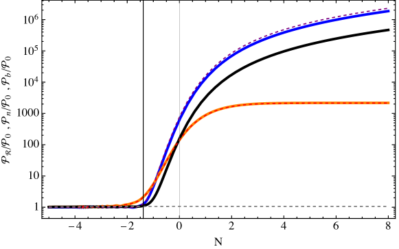
Figure 1: The power spectra (normalized by the single-field spectrum ${\cal{P}}_{0}$) for a given mode that crosses the horizon at $N=0$. The turning rate and torsion are zero before $N=-3$, and become constant afterwards. The three perturbations, $\mathcal{R}$, $q_{\rm n}/\sqrt{2\epsilon}$ and $q_{\rm b}/\sqrt{2\epsilon}$, all with the Bunch-Davies initial conditions, are depicted in thin dashed purple, red and gray respectively for the model without torsion, and in thick solid blue, orange and black respectively for the model with torsion. After the horizon crossing the normal perturbation $q_{\rm n}$ freezes whereas the curvature perturbation $\mathcal{R}$ continues to increase. The behaviour of the binormal perturbation $q_{\rm b}$ depends on the value of the torsion: For the zero torsion case it is effectively decoupled from the other two and behaves as a single-field perturbation, whereas for the non-zero case it continues to increase on superhorizon scales. The vertical line at $N\approx-1.5$ corresponds to the $e$-folding time when (80) is satisfied and the exponential amplification of perturbations commences.

V Analytic solutions for sharp and broad turns

To gain further physical insights, in this section we consider a simple two-field system that undergoes a sharp or broad turn. We can find a set of analytic solutions of perturbations, and in particular can identify how the positive eigenvalues enhance the perturbations. Note that while we use Hamilton’s equations to study the behaviour of the two perturbations, we have checked that our results for a single turn are consistent with Palma:2020ejf ; Fumagalli:2020nvq for the sharp turn case. For the broad turn case we revisit some of the assumptions made in Bjorkmo:2019qno and clarify the role of the Hubble friction terms in the derivation of the analytic solutions.

V.1 Sharp turns

For two fields, the $4\times 4$ system of the fields and their conjugate momenta is the following:

$$\mathcal{R}^{\prime} =P_{\mathcal{R}}+2\Omega\mathcal{S}\,,$$ (95)

$$P_{\mathcal{R}}^{\prime} =-(3-\epsilon+\eta)P_{\mathcal{R}}-\kappa^{2}\mathcal{R}\,,$$ (96)

$$\mathcal{S}^{\prime} =P_{\mathcal{S}}\,,$$ (97)

$$P_{\mathcal{S}}^{\prime} =-2\Omega P_{\mathcal{R}}-(3-\epsilon+\eta)P_{\mathcal{S}}-\left[\kappa^{2}+m_{\rm eff}+{1\over 2}\eta\left(3-\epsilon+{1\over 2}\eta\right)+{1\over 2}\eta^{\prime}\right]\mathcal{S}\,,$$ (98)

where we used the entropic perturbation $\mathcal{S}\equiv q_{\rm n}/\sqrt{2\epsilon}$. Now, we assume that the turn is finite, i.e. the turn occurs within a finite duration of time and that $|\eta|\ll 1$. Since the duration of the turn is finite, the two perturbations are independent before the turn so we assign the Bunch-Davies initial conditions to both of them. After the turn, the two perturbations are decoupled again and are given as a superposition of Bessel functions of the first and second type:

$$\mathcal{R} ={\mathcal{R}|_{\rm te}\over\kappa_{\rm te}}\left(\kappa\cos\left(\kappa-\kappa_{\rm te}\right)-\sin\left(\kappa-\kappa_{\rm te}\right)\right)+{P_{\mathcal{R}}|_{\rm te}\over\kappa_{\rm te}^{3}}\left[\left(\kappa-\kappa_{\rm te}\right)\cos\left(\kappa-\kappa_{\rm te}\right)-(1+\kappa\kappa_{\rm te})\sin\left(\kappa-\kappa_{\rm te}\right)\right]\,,$$ (99)

$$\mathcal{S} ={\pi\kappa^{3/2}\over 2\kappa_{\rm te}^{3/2}}\left\{\left[\mathcal{S}|_{\rm te}\left(\nu-{3\over 2}\right)+P_{\mathcal{S}}|_{\rm te}\kappa_{\rm te}\right]J_{\nu}(\kappa_{\rm te})-\mathcal{S}|_{\rm te}\kappa_{\rm te}J_{\nu-1}(\kappa_{\rm te})\right\}Y_{\nu}(\kappa)$$

$$\quad+{\pi\kappa^{3/2}\over 2\kappa_{\rm te}^{3/2}}\left\{\left[\mathcal{S}|_{\rm te}\left(\nu-{3\over 2}\right)+P_{\mathcal{S}}|_{\rm te}\kappa_{\rm te}\right]Y_{\nu}(\kappa_{\rm te})-\mathcal{S}|_{\rm te}\kappa_{\rm te}Y_{\nu-1}(\kappa_{\rm te})\right\}J_{\nu}(\kappa)\,,$$ (100)

where

$$\nu\equiv\sqrt{{9\over 4}-\mathcal{M}_{\rm nn}}\,,$$ (101)

and the subscript “te” denotes the values at the end of the turn. Setting $\kappa=0$ in the above relations gives the asymptotic values for the two perturbations which depend on the the values of the two perturbations and their momenta at the end of the turn.

During the turn the two perturbations become coupled and one has to solve the $4\times 4$ non-autonomous system of equations. We model the turn with the step function $\Theta$:

$$\Omega={\delta\theta\over\delta N}\left[\Theta\left(N-N_{\rm ti}\right)-\Theta\left(N-N_{\rm te}\right)\right]\,,$$ (102)

where $\delta\theta\equiv\int^{N_{\rm te}}_{N_{\rm ti}}\Omega\,\,\mathrm{d}N$ is the total angle swept during the turn and $\delta N\equiv N_{\rm te}-N_{\rm ti}$ is the duration of the turn. The general solution at the end of the turn is given by the time-ordered exponential, which can be represented as a Dyson series

$$X(N_{\rm te})=\left[I+\int^{N_{\rm te}}_{N_{\rm ti}}\,\mathrm{d}N_{1}J(N_{1})+{1\over 2}\int^{N_{\rm te}}_{N_{\rm ti}}\int^{N_{1}}_{N_{\rm ti}}\,\mathrm{d}N_{2}\,\mathrm{d}N_{1}J(N_{1})J(N_{2})+\cdots\right]X_{0}\,.$$ (103)

Since $J$ has no oscillating part, when the duration of the turn is small we can approximate every integral with a rectangle as

$$X(N_{\rm te})=I+\delta NJ(N_{*})+{1\over 2}(\delta N)^{2}J(N_{*})J(N_{*})+\cdots=\exp\left[J(N_{*})\delta N\right]\,,$$ (104)

where $N_{*}$ can in principle be any value lying in the interval $\left[N_{\rm ti},N_{\rm te}\right]$ (usually the middle value yields better numerical results). The solution is then found by diagonalizing $J(N_{*})$, with $J(N_{*})=U^{-1}J_{\rm D}U$, and expressing it as a linear combination of the eigenvectors of $U$ multiplied by exponentials:

$$X=\sum_{i}c_{i}\exp(\lambda_{i}N)\,\bm{e}_{i}\,,$$ (105)

where $c_{i}$ are found from the initial conditions, the eigenvectors are

$$\bm{e}_{i}=\begin{pmatrix}1\vspace{0.4em}\\ -\dfrac{\kappa^{2}}{\bar{\lambda}_{i}}\vspace{0.4em}\\ \dfrac{\kappa^{2}+\lambda_{i}\bar{\lambda}_{i}}{2\Omega\bar{\lambda}_{i}}\vspace{0.4em}\\ \lambda_{i}\dfrac{\kappa^{2}+\lambda_{i}\bar{\lambda}_{i}}{2\Omega\bar{\lambda}_{i}}\end{pmatrix}\,,$$ (106)

and $\lambda$’s are the diagonal elements of $J_{\rm D}$, explicitly given by

$$\lambda_{1,2,3,4} =-{1\over 2}\left[3-\epsilon\pm\sqrt{(3-\epsilon)^{2}-4\kappa^{2}-2m_{\rm eff}\pm 2\sqrt{m_{\rm eff}^{2}+16\kappa^{2}\Omega^{2}}}\right]\,,$$ (107)

$$\lambda_{1}+\lambda_{2}=\lambda_{3}+\lambda_{4} =-(3-\epsilon)\,,$$ (108)

$$\bar{\lambda}_{i} \equiv(3-\epsilon)+\lambda_{i}\,.$$ (109)

It is worth noticing that if we neglect the Hubble friction terms, which is usually taken when one considers the evolution of perturbations on subhorizon scales, the corresponding solutions are the same as the above without the factor $3-\epsilon$. We will return to this point later.

After the turn, the two perturbations decouple so that $\mathcal{R}$ freezes on the superhorizon scales. This value is given by $\mathcal{R}|_{\rm te}$ and $P_{\mathcal{R}}|_{\rm te}$. Since the system consists of linear differential equations, these values in turn depend linearly on the values of the four variables at the beginning of the turn, which we denote by the subscript “ti”. We can split $\mathcal{R}|_{\rm te}$ and $P_{\mathcal{R}}|_{\rm te}$ into two parts, one that we denote by the superscript $(\mathcal{R})$ being dependent on the initial curvature pair $\left(\mathcal{R}|_{\rm ti},P_{\mathcal{R}}|_{\rm ti}\right)$, and the other denoted by $(\mathcal{S})$ being determined by the initial isocurvature pair $\left(\mathcal{S}|_{\rm ti},P_{\mathcal{S}}|_{\rm ti}\right)$:

$$\mathcal{R}|_{\rm te} =\mathcal{R}^{(\mathcal{R})}|_{\rm te}+\mathcal{R}^{(\mathcal{S})}|_{\rm te}=\mathcal{R}^{(\mathcal{R})}|_{\rm te}\left(\mathcal{R}|_{\rm ti},P_{\mathcal{R}}|_{\rm ti}\right)+\mathcal{R}^{(\mathcal{S})}|_{\rm te}\left(\mathcal{S}|_{\rm ti},P_{\mathcal{S}}|_{\rm ti}\right)\,,$$ (110)

$$P_{\mathcal{R}}|_{\rm te} =P_{\mathcal{R}}^{(\mathcal{R})}|_{\rm te}+P_{\mathcal{R}}^{(\mathcal{S})}|_{\rm te}=P_{\mathcal{R}}^{(\mathcal{R})}|_{\rm te}\left(\mathcal{R}|_{\rm ti},P_{\mathcal{R}}|_{\rm ti}\right)+P_{\mathcal{R}}^{(\mathcal{S})}|_{\rm te}\left(\mathcal{S}|_{\rm ti},P_{\mathcal{S}}|_{\rm ti}\right)\,,$$ (111)

with the following explicit expressions:

$$\mathcal{R}^{(\mathcal{R})}|_{\rm te} \equiv{\left(\kappa^{2}-\lambda_{3}\lambda_{4}\right)\left[\lambda_{2}e^{\lambda_{1}\delta N}\left(\lambda_{1}P_{\mathcal{R}}|_{\rm ti}-\kappa^{2}\mathcal{R}|_{\rm ti}\right)-\lambda_{1}e^{\lambda_{2}\delta N}\left(\lambda_{2}P_{\mathcal{R}}|_{\rm ti}-\kappa^{2}\mathcal{R}|_{\rm ti}\right)\right]\over\kappa^{2}(\lambda_{2}-\lambda_{4})(\lambda_{1}-\lambda_{4})(\lambda_{1}-\lambda_{2})}$$

$$\quad+{\left(\kappa^{2}-\lambda_{1}\lambda_{2}\right)\left[\lambda_{4}e^{\lambda_{3}\delta N}\left(\lambda_{3}P_{\mathcal{R}}|_{\rm ti}-\kappa^{2}\mathcal{R}|_{\rm ti}\right)-\lambda_{3}e^{\lambda_{4}\delta N}\left(\lambda_{4}P_{\mathcal{R}}|_{\rm ti}-\kappa^{2}\mathcal{R}|_{\rm ti}\right)\right]\over\kappa^{2}(\lambda_{2}-\lambda_{4})(\lambda_{1}-\lambda_{4})(\lambda_{4}-\lambda_{3})}\,,$$ (112)

$$\mathcal{R}^{(\mathcal{S})}|_{\rm te} \equiv{2\Omega\left[\lambda_{2}e^{\lambda_{1}\delta N}\left(P_{\mathcal{S}}|_{\rm ti}-\lambda_{2}\mathcal{S}|_{\rm ti}\right)-\lambda_{1}e^{\lambda_{2}\delta N}\left(P_{\mathcal{S}}|_{\rm ti}-\lambda_{1}\mathcal{S}|_{\rm ti}\right)\right]\over(\lambda_{2}-\lambda_{4})(\lambda_{1}-\lambda_{4})(\lambda_{1}-\lambda_{2})}$$

$$\quad+{2\Omega\left[\lambda_{4}e^{\lambda_{3}\delta N}\left(P_{\mathcal{S}}|_{\rm ti}-\lambda_{4}\mathcal{S}|_{\rm ti}\right)-\lambda_{3}e^{\lambda_{4}\delta N}\left(P_{\mathcal{S}}|_{\rm ti}-\lambda_{3}\mathcal{S}|_{\rm ti}\right)\right]\over(\lambda_{2}-\lambda_{4})(\lambda_{1}-\lambda_{4})(\lambda_{4}-\lambda_{3})}\,,$$ (113)

$$P_{\mathcal{R}}^{(\mathcal{R})}|_{\rm te} \equiv{\left(\kappa^{2}-\lambda_{3}\lambda_{4}\right)\left[e^{\lambda_{1}\delta N}\left(\lambda_{1}P_{\mathcal{R}}|_{\rm ti}-\kappa^{2}\mathcal{R}|_{\rm ti}\right)-e^{\lambda_{2}\delta N}\left(\lambda_{2}P_{\mathcal{R}}|_{\rm ti}-\kappa^{2}\mathcal{R}|_{\rm ti}\right)\right]\over(\lambda_{2}-\lambda_{4})(\lambda_{1}-\lambda_{4})(\lambda_{1}-\lambda_{2})}$$

$$\quad+{\left(\kappa^{2}-\lambda_{1}\lambda_{2}\right)\left[e^{\lambda_{3}\delta N}\left(\lambda_{3}P_{\mathcal{R}}|_{\rm ti}-\kappa^{2}\mathcal{R}|_{\rm ti}\right)-e^{\lambda_{4}\delta N}\left(\lambda_{4}P_{\mathcal{R}}|_{\rm ti}-\kappa^{2}\mathcal{R}|_{\rm ti}\right)\right]\over(\lambda_{2}-\lambda_{4})(\lambda_{1}-\lambda_{4})(\lambda_{4}-\lambda_{3})}\,,$$ (114)

$$P_{\mathcal{R}}^{(\mathcal{S})}|_{\rm te} \equiv{2\Omega\kappa^{2}\left[e^{\lambda_{1}\delta N}\left(P_{\mathcal{S}}|_{\rm ti}-\lambda_{2}\mathcal{S}|_{\rm ti}\right)-e^{\lambda_{2}\delta N}\left(P_{\mathcal{S}}|_{\rm ti}-\lambda_{1}\mathcal{S}|_{\rm ti}\right)\right]\over(\lambda_{2}-\lambda_{4})(\lambda_{1}-\lambda_{4})(\lambda_{1}-\lambda_{2})}$$

$$\quad+{2\Omega\kappa^{2}\left[e^{\lambda_{3}\delta N}\left(P_{\mathcal{S}}|_{\rm ti}-\lambda_{4}\mathcal{S}|_{\rm ti}\right)-e^{\lambda_{4}\delta N}\left(P_{\mathcal{S}}|_{\rm ti}-\lambda_{3}\mathcal{S}|_{\rm ti}\right)\right]\over(\lambda_{2}-\lambda_{4})(\lambda_{1}-\lambda_{4})(\lambda_{4}-\lambda_{3})}\,.$$ (115)

Here, for $\kappa$ in principle we can use any value between $\kappa_{\rm te}$ and $\kappa_{\rm ti}$, but numerically we find that the value corresponding to $\delta N/2$ is more accurate (corresponding to the better finite difference approximation scheme of $\int\,\mathrm{d}N^{\prime}J$). This split becomes very useful when quantizing the two perturbations.

Having found the analytic solutions, now we proceed to compute the power spectrum at the end of inflation. For this goal, we promote the fields to operators and decompose them in terms of the creation and annihilation operators, and solve for the vacuum state mode functions. Then, the power spectrum is obtained by the absolute value squared of the mode function evaluated at the end of inflation. For the current case, the sensible moment to set up the operators is well before the horizon crossing where we can treat both $\mathcal{R}$ and $\mathcal{S}$ quantum mechanically. Thus, the two independent degrees of freedom at early stage are $\mathcal{R}|_{\text{ti}}$ and $\mathcal{S}|_{\text{ti}}$ that can be written in terms of the Bunch-Davies mode function solutions. Consequently, the two asymptotic values for the curvature perturbation (99) for $\kappa\to 0$ can be divided into two parts with one being dependent only on $\mathcal{R}^{(\mathcal{R})}|_{\text{te}}$ and $P_{\mathcal{R}}^{(\mathcal{R})}|_{\text{te}}$, and the other only on $\mathcal{R}^{(\mathcal{S})}|_{\text{te}}$ and $P_{\mathcal{R}}^{(\mathcal{R})}|_{\text{te}}$:

$$\mathcal{R}^{(\mathcal{R})}(\kappa\to 0) ={\mathcal{R}^{(\mathcal{R})}|_{\rm te}\over\kappa_{\rm te}}\sin\left(\kappa_{\rm te}\right)+{P_{\mathcal{R}}^{(\mathcal{R})}|_{\rm te}\over\kappa_{\rm te}^{3}}\left[\sin\left(\kappa_{\rm te}\right)-\kappa_{\rm te}\cos\left(\kappa_{\rm te}\right)\right]\,,$$ (116)

$$\mathcal{R}^{(\mathcal{S})}(\kappa\to 0) ={\mathcal{R}^{(\mathcal{S})}|_{\rm te}\over\kappa_{\rm te}}\sin\left(\kappa_{\rm te}\right)+{P_{\mathcal{R}}^{(\mathcal{S})}|_{\rm te}\over\kappa_{\rm te}^{3}}\left[\sin\left(\kappa_{\rm te}\right)-\kappa_{\rm te}\cos\left(\kappa_{\rm te}\right)\right]\,,$$ (117)

from which we find the power spectrum as

$$\mathcal{P}_{\mathcal{R}}={k^{3}\over 2\pi^{2}}\left[\left|\mathcal{R}^{(\mathcal{R})}(\kappa\to 0)\right|^{2}+\left|\mathcal{R}^{(\mathcal{S})}(\kappa\to 0)\right|^{2}\right]\,.$$ (118)

In figure 2 we verify the accuracy of our analytic estimate for the power spectrum by plotting the amplification (relative to the single-field result) of the power spectrum for a given mode. For the specific choice of parameters we observe an amplification of almost 6 orders of magnitude, with the analytic result being perfectly consistent with full numerical one.

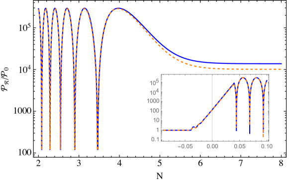
Figure 2: The evolution of the curvature perturbation (normalized by the single-field expression $\mathcal{P}_{0}$) for a sharp turn (taking the form of a top-hat function) of total swapped angle $4\pi$ and duration $\delta N=0.1$ $e$-folds. The effective mass has been chosen as $m_{\rm eff}=2\Omega^{2}+5$ and the turn is centred around $N=0$. The two curves correspond to the numerical solution (solid) and the approximate analytic one (dashed) given by the series of formulae presented in section V.1. The negligible difference from around the horizon-crossing point ($N\sim 5$) is due to neglecting the slow-roll parameters in the analytic approximation.

V.2 Broad turns

When the turn is sufficiently long in duration, the situation is drastically different. Looking at the formal expression (103) it becomes clear that in principle one has to use the full Dyson series to obtain a reliable solution, though in most cases some perturbative scheme is assumed and the Dyson series is truncated at a given order. In this subsection we will show how this is done in the case of constant and large turns.

The first (approximate) analytic solution in the case of constant turns was presented in Bjorkmo:2019qno under certain assumptions. First, it relied on the effective field theory description of Garcia-Saenz:2018vqf which predicted a power spectrum at the end of inflation given as $\mathcal{P}=\mathcal{P}_{0}e^{2x}$, with $\mathcal{P}_{0}$ being the single-field power spectrum and $x$ an unknown constant that is derived from the full two-field theory. Second, the Hubble friction terms were assumed negligible on subhorizon scales, an assumption that was also present in predecessor works on the effective field theory for constant turns e.g. Achucarro:2012yr . Lastly, by pointing out the stability matrix of the coupled $\mathcal{R}$-$\mathcal{S}$ differential system (without the friction terms) acquires a positive eigenvalue at a given time before horizon crossing, the unknown constant $x$ is identified as $\int\,\mathrm{d}N\lambda_{4}$, where $\lambda_{4}$ corresponds to the eigenvalue that becomes positive. Even though the solution was obtained as an approximation it matched numerics to a great accuracy.

However, examining the role of the Hubble friction terms in more detail leads to an apparent contradiction. If the Hubble friction terms are subdominant then on similar grounds one might expect that including those terms into the definition of the fourth eigenvalue would yield more accurate results. Surprisingly though, the more accurate version of the fourth eigenvalue [which we have listed in (107)] severely underestimates the overall amplification by an amount that is beyond the expected accuracy of the method. This happens because the eigenvalue including the friction terms has the form $-(3-\epsilon)+\sqrt{(3-\epsilon)^{2}+A}$, in contrast to the one without the friction terms $\sqrt{A}$ and thus falls off faster as $A$ decreases, i.e. as the mode approaches the horizon, leading to significantly less amplification. This also has the implication that for small $\kappa$ the dominant $\kappa$-dependent part of $\log\mathcal{P}$ takes the form $|c_{\rm s}^{2}|\kappa^{2}$ for the former case, with $c_{\rm s}^{2}$ being the sound speed in the effective description, as opposed to $|c_{\rm s}|\kappa$ for the latter case which is also the correct result. Therefore, to derive the correct formula one has to omit the Hubble friction terms, which seems self-contradicting.

The role of the friction terms is important even for subhorizon scales as they control the amplitude of oscillations. As we show in appendix B, solving the single-field curvature perturbation without the friction terms yields the wrong result: Specifically $|\mathcal{R}|\rightarrow 0$ for $N\rightarrow-\infty$ instead of the correct value $|\mathcal{R}|\sim e^{-N}$. Even though a case could be made that these terms would yield sub-leading corrections for large turns, in reality for this to hold one should consider extreme turns of the order $\mathcal{O}(300)$, well outside the validity of perturbation theory. In what follows we will derive an approximate solution for $\mathcal{R}$ as well as for $\mathcal{S}$, which was not derived in the previous references, without resorting to an effective field theory approach. This will be done by converting the equations for perturbations into perturbative expansion in terms of $\kappa^{-1}$ and find a consistent solution for the zeroth-order part. Moreover, we clarify the role of the Hubble friction terms which, when taken into account, amounts for the correct amplitude at horizon crossing.

For broad turns we are interested in finding an analytic solution for subhorizon scales, so we will first recast the system in a perturbative form with $\kappa^{-1}$ being our expansion parameter. More specifically, we perform the change of variables $N\rightarrow x$ with $x$ being defined in (28), redefine the momenta $P\rightarrow-x\tilde{P}$ and obtain

$$\mathcal{R}_{,x} =\tilde{P}_{\mathcal{R}}-{2\Omega\over x}\mathcal{S}\,,$$ (119)

$$\tilde{P}_{\mathcal{R},x} ={2\over x}\tilde{P}_{\mathcal{R}}-\mathcal{R}\,,$$ (120)

$$\mathcal{S}_{,x} =\tilde{P}_{\mathcal{S}}\,,$$ (121)

$$\tilde{P}_{\mathcal{S},x} ={2\Omega\over x}\tilde{P}_{\mathcal{R}}+{2\over x}\tilde{P}_{\mathcal{S}}-\left(1+{m_{\rm eff}\over x^{2}}\right)\mathcal{S}\,.$$ (122)

See appendix B for more details and motivation for the method. For the latter system the stability matrix splits into two parts:

$$X_{,x}=J_{(0)}X+J_{(1)}X\,,$$ (123)

where $J_{(0)}$ is the dominant part, which may be $x$-dependent, and $J_{(1)}$ contains subdominant terms suppressed by $x^{-1}$. Except for the Hubble friction terms which are always suppressed, the coupling terms containing the turn rate may fall on either part of the stability matrix depending on the regime of interest. Assuming that the turn rate is large $\Omega\gg 1$ there are effectively three regimes:

1. $\Omega\ll x$, where both the Hubble friction and the coupling terms are subdominant;

2. $\Omega\sim x$, which is roughly the period when most of the amplification takes place;

3. $\Omega\gg x$, which is the regime of validity of the effective single-field description.

The next step is to redefine $X$ as $X\equiv UY$, where the matrix $U$ diagonalizes $J_{(0)}$ via $J_{\rm D}=U^{-1}J_{(0)}U$ and obtain a new equation

$$Y_{,x}=J_{\rm D}Y+\left(U^{-1}J_{(1)}U-U^{-1}U_{,x}\right)Y\,.$$ (124)

By using this transformation we have reduced the problem to a zeroth-order diagonal part plus a perturbation term, and our goal is to consistently solve the zeroth-order part only. This, however, does not mean we can discard entirely this perturbation term. Since the diagonalization matrix $U$ is not uniquely defined, the zeroth-order solution for $Y$ is ambiguous. To completely remove this ambiguity, we note that for $U$ we have the freedom to multiply each of its columns by an arbitrary function, which amounts to rescaling the eigenvectors of $J_{(0)}$. Thus we can choose $U$ in such a way that the subdominant term in (124) has only non-diagonal elements. This is equivalent to taking into account the diagonal elements of zeroth- and first-order when solving for $Y$. For completeness, we list the eigenvalues of $J_{(0)}$:

$$\lambda_{\rm im} =\pm{i\over\sqrt{2}x}\sqrt{2x^{2}+m_{\rm eff}+\sqrt{m_{\rm eff}^{2}+16x^{2}\Omega^{2}}}\,,$$ (125)

$$\lambda_{\rm p} =\pm{1\over\sqrt{2}x}\sqrt{-2x^{2}-m_{\rm eff}+\sqrt{m_{\rm eff}^{2}+16x^{2}\Omega^{2}}}\,,$$ (126)

where the subscript “im” reflects the fact that the first two eigenvalues are always imaginary, whereas $\lambda_{\rm p}$ with the plus sign becomes positive for $x^{2}<4\Omega-m_{\rm eff}$. Putting all these together we find the general solution for $\mathcal{R}$ and $\mathcal{S}$ as

$$\mathcal{R} =xf_{+}(x)\left(c_{1}e^{-\int\lambda_{\rm im}}+c_{2}e^{\int\lambda_{\rm im}}\right)+xf_{-}(x)\left(c_{3}e^{-\int\lambda_{\rm p}}+c_{4}e^{\int\lambda_{\rm p}}\right)\,,$$ (127)

$$\mathcal{S} =xf_{+}(x)s_{\rm im}\left(c_{1}e^{-\int\lambda_{\rm im}}-c_{2}e^{\int\lambda_{\rm im}}\right)+xf_{-}(x)s_{\rm p}(x)\left(-c_{3}e^{-\int\lambda_{\rm p}}+c_{4}e^{\int\lambda_{\rm p}}\right)\,,$$ (128)

where $f_{\pm}(x)$ and $s_{{\rm im}({\rm p})}(x)$ are given by

$$f_{\pm}(x) \equiv\left[1-{4\Omega^{2}\pm m_{\rm eff}\over\sqrt{m_{\rm eff}^{2}+16x^{2}\Omega^{2}}}-{4\Omega^{2}(2x^{2}\mp m)\over m_{\rm eff}^{2}+16x^{2}\Omega^{2}}\right]^{1/4}\,,$$ (129)

$$s_{{\rm im}({\rm p})}(x) \equiv{x\big{(}\lambda_{{\rm im}({\rm p})}^{2}+1\big{)}\over 2\Omega\lambda_{{\rm im}({\rm p})}}\,.$$ (130)

The solution is ill-behaved for $x\rightarrow 0$ and $x\to\sqrt{4\Omega^{2}-m_{\rm eff}}$. This is because at these points $J_{(0)}$ becomes non-diagonalizable and subsequently the transformation $X\rightarrow Y$ is also ill-defined. This is an artifact of our parameterization and we can assume a regularization scheme. The inconsistency at the superhorizon limit $x\rightarrow 0$ can be fixed by replacing the overall $x$ term by $x+i$, similar to what we can do for single field as we show in appendix B. For $x\rightarrow\sqrt{4\Omega^{2}-m}$ the two functions $f_{-}$ and $s_{\rm p}$ go to zero, yielding another problem for both the perturbations and their derivatives. Away from this point this function is almost constant so we can regularize it similarly by replacing $f_{-}=(\cdots)^{1/4}\rightarrow(i+\cdots)^{1/4}$. At horizon crossing these functions yield $\mathcal{O}(1)$ corrections so we can ignore them and quote the final result for the curvature pertuarbation at horizon crossing:

$$\mathcal{P}_{\mathcal{R}}\approx\mathcal{P}_{0}|f_{-}|^{2}\left.\exp\left(2\int_{\sqrt{4\Omega^{2}-m_{\rm eff}}}^{1}\,\mathrm{d}x\lambda_{\rm p}\right)\right|_{x=1}\,.$$ (131)

Note that taking the limit $x\rightarrow 0$ in the above integral yields the amplification factor $\pi\Omega\left(2-\sqrt{m_{\rm eff}}/\Omega\right)$ that was mentioned in Bjorkmo:2019qno . The expression for the isocurvature perturbation is qualitatively correct but accurate only up to the point where the isocurvature mass has reached its maximum value, and after that it predicts smaller rate of decrease. The decrease comes from the factor $x$ in (130) and so the approximation predicts $\mathcal{S}\propto x$. Parameterizing the effective mass as $m_{\rm eff}=(3+b)\Omega^{2}$, and keeping in mind that the exponential amplification is possible only for $b\in[-3,1)$, (128) becomes more accurate for $b\rightarrow-3$ up to horizon crossing, since in this case the perturbation keeps increasing, while in other cases the accuracy drops as we enter the effective single-field description, without affecting the accuracy of the formula for the curvature perturbation.

VI Conclusions

Multiple fields are ubiquitous in models inspired by high-energy theories of the early universe. Besides their non-trivial dynamics they may display interesting phenomenologies with large deviations from the standard slow-roll predictions. In the rapid-turn regime this class of models has been shown to generate an exponential amplification of the power spectrum on small scales, while keeping almost scale invariance on the CMB scales, a mechanism that can be used to lead to PBH formation. In this work we explored this idea further, and below we summarize our main results.

More specifically, in section II we introduced the basic ingredients of multi-field perturbations and showed that a simple change of the variable $x\equiv-k\tau$ trivially yields the scale dependence of the power spectrum when every background quantity is constant, without resorting to an effective field theory or to the slow-turn limit. Then, in section III we pointed out that the behaviour of perturbations becomes more transparent in the Hamiltonian description and we investigated under what general conditions the curvature perturbation becomes exponentially enhanced on subhorizon scales, and when the perturbations remain stable on superhorizon scales. We applied our findings on three-field models with isometries in section IV and showed that the amplification happens when the quantity $\mathcal{M}_{\rm nn}-\Omega^{2}-T^{2}$ becomes negative, very analogous to the two-field case. We continued with a discussion of the ultra light scenario with all three fields being massless on superhorizon scales and showed that when the torsion of the trajectory in the field space is non-zero then, in addition to the curvature perturbation, the binormal perturbation is also continuously sourced by the normal perturbation, the latter being constant. This partly answers the question of whether the presence of the torsion can produce distinct observational signatures in models with more than two fields.

Lastly, in section V we quantified the enhancement of perturbations for two-field systems that undergo constant turns. More specifically, for sharp turns the solution is found by exponentiating the stability matrix of perturbations, while for broad turns one has to first write the system into perturbative expansion over $1/x$ and then try to solve it perturbatively. In the latter case for solutions of the form $A\exp(B)$ the phase $B$, which can be either imaginary or real, is found by solving the part of the equations without the Hubble friction terms, while the correct amplitude is found only once the Hubble friction terms are taken into account. Although we have limited our discussion on two fields, it is straightforward to generalize our results for more fields. We also refer the interested readers to Aragam:2023adu where the authors studied the amplification of the power spectrum for three-field systems due to a sudden increase of the turn rate and torsion.

Appendix A Massive field in quasi-de Sitter space

The curvature perturbation in single-field inflation is a massless scalar field in the sense that it freezes on superhorizon scales. To find the approximate analytic solution it is better to switch to the canonical field $u=\sqrt{2\epsilon}\mathcal{R}$ which obeys the Mukhanov-Sasaki equation Sasaki:1986hm ; Mukhanov:1988jd :

$$u_{,\tau\tau}+\left[k^{2}-(aH)^{2}\left(2-\epsilon+{3\over 2}\eta-{1\over 2}\epsilon\eta+{1\over 4}\eta^{2}+{1\over 2}\eta\xi\right)\right]u=0\,,$$ (132)

with $\xi\equiv(\log\eta)^{\prime}$. The term $aH$ is related to the conformal time via

$$\tau-\tau_{\rm r}=\int^{N}_{N_{\rm r}}\,\mathrm{d}{N}^{\prime}{1\over aH}=\int^{N}_{N_{\rm r}}\,\mathrm{d}{N}^{\prime}{1\over a_{0}}e^{-{N}^{\prime}+\int\,\mathrm{d}n\epsilon(n)}\,,$$ (133)

where the last expression follows from the definition of the slow-roll parameter $\epsilon\equiv-(\log H)^{\prime}$ and for de Sitter space we follow the convention $\tau_{\rm r}\rightarrow 0$ for $N_{\rm r}\rightarrow\infty$. Integrating by parts twice yields

$$\tau-\tau_{\rm r}=-{1+\epsilon\over aH}\Big{|}^{N}_{N_{\rm r}}+\int\,\mathrm{d}{N}^{\prime}{\epsilon^{2}+\epsilon\eta\over aH}\,,$$ (134)

where the second term is at least one order higher in the slow-roll parameters. To first order in the slow-roll parameters (132) becomes

$$u_{,\tau\tau}+\left[k^{2}-{1\over\tau^{2}}\left(2+3\epsilon+{3\over 2}\eta\right)\right]u=0\,,$$ (135)

with the solutions being the Hänkel functions of first and second type. Choosing the positive frequency solution at early times yields

$$u={1\over 2}\sqrt{\pi}e^{i(2\nu+1)\pi/4}\sqrt{-\tau}H^{(1)}_{\nu}(\tau)\,,$$ (136)

with $\nu=3/2+\epsilon+\eta/2$. The same form of the solution holds for a massive field with mass term $\mathcal{M}_{\rm nn}$ upon replacing $\nu$ with

$$\nu=\sqrt{{9\over 4}-\mathcal{M}_{\rm nn}}\,.$$ (137)

Appendix B Perturbative diagonalization for systems of differential equations

In this section we present a method to generate approximate solutions for systems of first-order equations. For the simplest case of single field we write the equation for the curvature perturbation as

$$\mathcal{R}^{\prime} =P_{\mathcal{R}}\,,$$ (138)

$$P_{\mathcal{R}}^{\prime} =-(3-\epsilon+\eta)P_{\mathcal{R}}-\kappa^{2}\mathcal{R}\,.$$ (139)

We are interested in finding the solution for $\kappa\gg 1$ and to this end we perform the change of variables $\kappa\,\mathrm{d}N=-\,\mathrm{d}\kappa$ that transforms the system into a perturbative expansion in terms of $1/\kappa$. Ignoring slow-roll corrections we find $\kappa\approx x$, where $x$ was defined in (28). Dividing the second equation with $x^{2}$ and performing the change of variables we obtain

$$-{\,\mathrm{d}\mathcal{R}\over\,\mathrm{d}x} ={P_{\mathcal{R}}\over x}\,,$$ (140)

$$-{1\over x}{\,\mathrm{d}P_{\mathcal{R}}\over\,\mathrm{d}x} =-{3\over x^{2}}P_{\mathcal{R}}-\mathcal{R}\,.$$ (141)

The second equation implies that we need to redefine $P_{\mathcal{R}}$ as $P_{\mathcal{R}}\equiv-x\tilde{P}_{\mathcal{R}}$ so that its derivative is not multiplied with the small parameter, then we obtain

$${\,\mathrm{d}\tilde{P}_{\mathcal{R}}\over\,\mathrm{d}x}={2\over x}\tilde{P}_{\mathcal{R}}-\mathcal{R}\,.$$ (142)

The new set of equations is written in perturbative form

$$X_{,x}=J_{(0)}X+J_{(1)}X\,,$$ (143)

where now

$$X\equiv\begin{pmatrix}\mathcal{R}\\ \tilde{P}_{\mathcal{R}}\end{pmatrix}\,,\qquad J_{(0)}\equiv\begin{pmatrix}0&1\\ -1&0\end{pmatrix}\,,\qquad J_{(1)}\equiv\begin{pmatrix}0&0\\ 0&{2\over x}\end{pmatrix}\,.$$ (144)

The next step is to diagonalize the zeroth-order stability matrix as $J_{\rm D}\equiv U^{-1}J_{(0)}U$ and rewrite (143) in terms of the new variable $X\equiv UY$:

$$Y_{,x}=J_{\rm D}Y+U^{-1}J_{(1)}UY-U^{-1}U_{,x}Y\,.$$ (145)

The last term is differentiated by $x$ and is hence first-order in terms of $x^{-1}$. Note that the $U$ matrix is not unique but it is defined up to arbitrary rescalings of its columns, which correspond to the eigenvectors of $J_{(0)}$. Therefore, it is not correct to ignore the higher-order diagonal terms in (145) because $X$ will be ambiguous as it depends on the choice of $U$. To break the degeneracy we will redefine $U$ such that there are no higher-order diagonal terms and then solve the lowest-order part of (145). This redefinition can be shown to be

$$\tilde{U}=U\exp\left(\int\,\mathrm{d}xJ_{\rm D(1)}\right)\,,\,$$ (146)

where by $J_{\rm D(1)}$ we denote a diagonal matrix constructed by the diagonal elements of $U^{-1}J_{(1)}U-U^{-1}U_{,x}$.

For our previous example we find the eigenvectors of $J_{(0)}$ as $e_{1}=(-i,1)^{T}$, $e_{2}=(i,1)^{T}$ and the diagonal higher-order terms of elements of (145) as $\text{diag}(1/x,1/x)$. Therefore, by defining the matrix $U$ as

$$U=\begin{pmatrix}-ix&x\\ ix&x\end{pmatrix}\,,$$ (147)

we find the fundamental matrix (i.e. the matrix of linearly independent solutions) of the lowest-order solution as

$$F_{Y}=\text{diag}\left(e^{ix},e^{-ix}\right)\,,$$ (148)

and subsequently the fundamental matrix of our original problem via $F_{X}=UF_{Y}$. Therefore, we find the general solution for the curvature perturbation as

$$\mathcal{R}=c_{1}xe^{ix}+c_{2}xe^{-ix}\,,$$ (149)

which is accurate up to $\mathcal{O}(1)$ corrections. It should also be clear that the Hubble friction terms provide the correct linear dependence on $x$, even though they are suppressed in the $x^{-1}$ expansion. This happens because they contribute $\log x$ corrections on the final result and thus cannot be consistently ignored in the final result even to leading order.

Finally, we should mention that the approximate solution (149) coincides with the WKB solution applied on the second-order equation

$$\mathcal{R}^{\prime\prime}+3\mathcal{R}^{\prime}+\kappa^{2}\mathcal{R}=0\,,$$ (150)

when considering an asymptotic expansion $\mathcal{R}=\exp\left(\kappa\mathcal{R}_{(0)}+\mathcal{R}_{(1)}+\cdots\right)$ and keeping only the first two terms. Although for single field the standard WKB method is simpler, for more fields substituting the above asymptotic expressions would result into a coupled time-dependent system considerably more involved than the one we obtain with the method described in this section.

References

- (1) N. Aghanim et al. [Planck], “Planck 2018 results. VI. Cosmological parameters,” Astron. Astrophys. 641, A6 (2020) [erratum: Astron. Astrophys. 652, C4 (2021)] [arXiv:1807.06209 [astro-ph.CO]].
- (2) A. A. Starobinsky, “A New Type of Isotropic Cosmological Models Without Singularity,” Phys. Lett. 91B, 99 (1980) [Adv. Ser. Astrophys. Cosmol. 3, 130 (1987)].
- (3) K. Sato, “Cosmological Baryon Number Domain Structure and the First Order Phase Transition of a Vacuum,” Phys. Lett. 99B, 66 (1981) [Adv. Ser. Astrophys. Cosmol. 3, 134 (1987)].
- (4) K. Sato, “First Order Phase Transition of a Vacuum and Expansion of the Universe,” Mon. Not. Roy. Astron. Soc. 195, 467 (1981).
- (5) D. Kazanas, “Dynamics of the Universe and Spontaneous Symmetry Breaking,” Astrophys. J. 241, L59 (1980).
- (6) A. H. Guth, “The Inflationary Universe: A Possible Solution to the Horizon and Flatness Problems,” Phys. Rev. D 23, 347 (1981) [Adv. Ser. Astrophys. Cosmol. 3, 139 (1987)].
- (7) A. D. Linde, “A New Inflationary Universe Scenario: A Possible Solution of the Horizon, Flatness, Homogeneity, Isotropy and Primordial Monopole Problems,” Phys. Lett. 108B, 389 (1982) [Adv. Ser. Astrophys. Cosmol. 3, 149 (1987)].
- (8) A. Albrecht and P. J. Steinhardt, “Cosmology for Grand Unified Theories with Radiatively Induced Symmetry Breaking,” Phys. Rev. Lett. 48, 1220 (1982) [Adv. Ser. Astrophys. Cosmol. 3, 158 (1987)].
- (9) Y. Akrami et al. [Planck], “Planck 2018 results. X. Constraints on inflation,” Astron. Astrophys. 641, A10 (2020) [arXiv:1807.06211 [astro-ph.CO]].
- (10) V. Mukhanov, “Physical Foundations of Cosmology,” Cambridge, UK: Univ. Pr. (2005) 421 p.
- (11) S. Weinberg, “Cosmology,” Oxford, UK: Oxford Univ. Pr. (2008) 593 p.
- (12) D. H. Lyth and A. R. Liddle, “The primordial density perturbation: Cosmology, inflation and the origin of structure,” Cambridge, UK: Cambridge Univ. Pr. (2009) 497 p.
- (13) J. E. Lidsey, A. R. Liddle, E. W. Kolb, E. J. Copeland, T. Barreiro and M. Abney, “Reconstructing the inflation potential : An overview,” Rev. Mod. Phys. 69, 373-410 (1997) [arXiv:astro-ph/9508078 [astro-ph]].
- (14) F. L. Bezrukov and M. Shaposhnikov, “The Standard Model Higgs boson as the inflaton,” Phys. Lett. B 659, 703-706 (2008) [arXiv:0710.3755 [hep-th]].
- (15) B. A. Bassett, S. Tsujikawa and D. Wands, “Inflation dynamics and reheating,” Rev. Mod. Phys. 78, 537-589 (2006) [arXiv:astro-ph/0507632 [astro-ph]].
- (16) D. Wands, “Multiple field inflation,” Lect. Notes Phys. 738, 275-304 (2008) [arXiv:astro-ph/0702187 [astro-ph]].
- (17) D. Langlois, “Lectures on inflation and cosmological perturbations,” Lect. Notes Phys. 800, 1-57 (2010) [arXiv:1001.5259 [astro-ph.CO]].
- (18) J. O. Gong, “Multi-field inflation and cosmological perturbations,” Int. J. Mod. Phys. D 26, no.01, 1740003 (2016) [arXiv:1606.06971 [gr-qc]].
- (19) J. Chluba, J. Hamann and S. P. Patil, “Features and New Physical Scales in Primordial Observables: Theory and Observation,” Int. J. Mod. Phys. D 24, no.10, 1530023 (2015) [arXiv:1505.01834 [astro-ph.CO]].
- (20) Y. Minami and E. Komatsu, “New Extraction of the Cosmic Birefringence from the Planck 2018 Polarization Data,” Phys. Rev. Lett. 125, no.22, 221301 (2020) [arXiv:2011.11254 [astro-ph.CO]].
- (21) J. R. Eskilt and E. Komatsu, “Improved constraints on cosmic birefringence from the WMAP and Planck cosmic microwave background polarization data,” Phys. Rev. D 106, no.6, 063503 (2022) [arXiv:2205.13962 [astro-ph.CO]].
- (22) S. M. Carroll, G. B. Field and R. Jackiw, “Limits on a Lorentz and Parity Violating Modification of Electrodynamics,” Phys. Rev. D 41, 1231 (1990).
- (23) A. G. Riess, S. Casertano, W. Yuan, L. M. Macri and D. Scolnic, “Large Magellanic Cloud Cepheid Standards Provide a 1% Foundation for the Determination of the Hubble Constant and Stronger Evidence for Physics beyond CDM,” Astrophys. J. 876, no.1, 85 (2019) [arXiv:1903.07603 [astro-ph.CO]].
- (24) V. Poulin, T. L. Smith, T. Karwal and M. Kamionkowski, “Early Dark Energy Can Resolve The Hubble Tension,” Phys. Rev. Lett. 122, no.22, 221301 (2019) [arXiv:1811.04083 [astro-ph.CO]].
- (25) B. P. Abbott et al. [LIGO Scientific and Virgo], “Observation of Gravitational Waves from a Binary Black Hole Merger,” Phys. Rev. Lett. 116, no.6, 061102 (2016) [arXiv:1602.03837 [gr-qc]].
- (26) Y. B. Zel’dovich and I. D. Novikov, “The Hypothesis of Cores Retarded during Expansion and the Hot Cosmological Model,” Soviet Astron. AJ (Engl. Transl. ), 10, 602 (1967).
- (27) S. Hawking, “Gravitationally collapsed objects of very low mass,” Mon. Not. Roy. Astron. Soc. 152, 75 (1971).
- (28) B. J. Carr and S. W. Hawking, “Black holes in the early Universe,” Mon. Not. Roy. Astron. Soc. 168, 399-415 (1974).
- (29) T. Harada, C. M. Yoo and K. Kohri, “Threshold of primordial black hole formation,” Phys. Rev. D 88, no.8, 084051 (2013) [erratum: Phys. Rev. D 89, no.2, 029903 (2014)] [arXiv:1309.4201 [astro-ph.CO]].
- (30) C. T. Byrnes, P. S. Cole and S. P. Patil, “Steepest growth of the power spectrum and primordial black holes,” JCAP 06, 028 (2019) [arXiv:1811.11158 [astro-ph.CO]].
- (31) S. Pi, Y. l. Zhang, Q. G. Huang and M. Sasaki, “Scalaron from -gravity as a heavy field,” JCAP 05, 042 (2018) [arXiv:1712.09896 [astro-ph.CO]].
- (32) G. A. Palma, S. Sypsas and C. Zenteno, “Seeding primordial black holes in multifield inflation,” Phys. Rev. Lett. 125, no.12, 121301 (2020) [arXiv:2004.06106 [astro-ph.CO]].
- (33) J. Fumagalli, S. Renaux-Petel and L. T. Witkowski, “Oscillations in the stochastic gravitational wave background from sharp features and particle production during inflation,” JCAP 08 (2021), 030 [arXiv:2012.02761 [astro-ph.CO]].
- (34) L. Anguelova, “On Primordial Black Holes from Rapid Turns in Two-field Models,” JCAP 06 (2021), 004 [arXiv:2012.03705 [hep-th]].
- (35) S. Bhattacharya and I. Zavala, “Sharp turns in axion monodromy: primordial black holes and gravitational waves,” JCAP 04 (2023), 065 [arXiv:2205.06065 [astro-ph.CO]].
- (36) J. Fumagalli, G. A. Palma, S. Renaux-Petel, S. Sypsas, L. T. Witkowski and C. Zenteno, “Primordial gravitational waves from excited states,” JHEP 03 (2022), 196 [arXiv:2111.14664 [astro-ph.CO]].
- (37) V. Aragam, S. Paban and R. Rosati, “Primordial Stochastic Gravitational Wave Backgrounds from a Sharp Feature in Three-field Inflation,” [arXiv:2304.00065 [astro-ph.CO]].
- (38) Y. F. Cai, X. Tong, D. G. Wang and S. F. Yan, “Primordial Black Holes from Sound Speed Resonance during Inflation,” Phys. Rev. Lett. 121, no.8, 081306 (2018) [arXiv:1805.03639 [astro-ph.CO]].
- (39) K. Boutivas, I. Dalianis, G. P. Kodaxis and N. Tetradis, “The effect of multiple features on the power spectrum in two-field inflation,” JCAP 08 (2022) no.08, 021 [arXiv:2203.15605 [astro-ph.CO]].
- (40) J. O. Gong and T. Tanaka, JCAP 03, 015 (2011) [erratum: JCAP 02, E01 (2012)] [arXiv:1101.4809 [astro-ph.CO]].
- (41) A. Achucarro, J. O. Gong, S. Hardeman, G. A. Palma and S. P. Patil, “Features of heavy physics in the CMB power spectrum,” JCAP 01 (2011), 030 [arXiv:1010.3693 [hep-ph]].
- (42) C. Gordon, D. Wands, B. A. Bassett and R. Maartens, “Adiabatic and entropy perturbations from inflation,” Phys. Rev. D 63 (2000), 023506 [arXiv:astro-ph/0009131 [astro-ph]].
- (43) A. Achucarro, J. O. Gong, S. Hardeman, G. A. Palma and S. P. Patil, “Effective theories of single field inflation when heavy fields matter,” JHEP 05 (2012), 066 [arXiv:1201.6342 [hep-th]].
- (44) E. Kreyszig, “Differential Geometry”, Dover Publications, 2013.
- (45) A. Achúcarro, S. Céspedes, A. C. Davis and G. A. Palma, “Constraints on Holographic Multifield Inflation and Models Based on the Hamilton-Jacobi Formalism,” Phys. Rev. Lett. 122 (2019) no.19, 191301 [arXiv:1809.05341 [hep-th]].
- (46) L. Pinol, “Multifield inflation beyond : non-Gaussianities and single-field effective theory,” JCAP 04 (2021), 002 [arXiv:2011.05930 [astro-ph.CO]].
- (47) Z. Lalak, D. Langlois, S. Pokorski and K. Turzynski, “Curvature and isocurvature perturbations in two-field inflation,” JCAP 07 (2007), 014 [arXiv:0704.0212 [hep-th]].
- (48) S. Cremonini, Z. Lalak and K. Turzynski, “Strongly Coupled Perturbations in Two-Field Inflationary Models,” JCAP 03 (2011), 016 [arXiv:1010.3021 [hep-th]].
- (49) J. O. Gong and E. D. Stewart, Phys. Lett. B 510, 1-9 (2001) [arXiv:astro-ph/0101225 [astro-ph]].
- (50) E. D. Stewart and D. H. Lyth, “A More accurate analytic calculation of the spectrum of cosmological perturbations produced during inflation,” Phys. Lett. B 302 (1993), 171-175 [arXiv:gr-qc/9302019 [gr-qc]].
- Barkovsky (2008) Y. S. Barkovsky, “Lectures on the Routh-Hurwitz problem,” [arXiv:0802.1805 [math.CA]].
- (52) P. Christodoulidis and R. Rosati, “(Slow-)twisting inflationary attractors,” JCAP 09 (2023), 034 [arXiv:2210.14900 [hep-th]].
- (53) A. Achúcarro, V. Atal, C. Germani and G. A. Palma, “Cumulative effects in inflation with ultra-light entropy modes,” JCAP 02 (2017), 013 [arXiv:1607.08609 [astro-ph.CO]].
- (54) P. Christodoulidis, D. Roest and E. I. Sfakianakis, “Attractors, Bifurcations and Curvature in Multi-field Inflation,” JCAP 08 (2020), 006 [arXiv:1903.03513 [gr-qc]].
- (55) A. Achúcarro, E. J. Copeland, O. Iarygina, G. A. Palma, D. G. Wang and Y. Welling, “Shift-symmetric orbital inflation: Single field or multifield?,” Phys. Rev. D 102 (2020) no.2, 021302 [arXiv:1901.03657 [astro-ph.CO]].
- (56) V. Aragam, S. Paban and R. Rosati, “Multi-field Inflation in High-Slope Potentials,” JCAP 04 (2020), 022 [arXiv:1905.07495 [hep-th]].
- (57) T. Bjorkmo, R. Z. Ferreira and M. C. D. Marsh, “Mild Non-Gaussianities under Perturbative Control from Rapid-Turn Inflation Models,” JCAP 12 (2019), 036 [arXiv:1908.11316 [hep-th]].
- (58) A. Achucarro, V. Atal, S. Cespedes, J. O. Gong, G. A. Palma and S. P. Patil, “Heavy fields, reduced speeds of sound and decoupling during inflation,” Phys. Rev. D 86 (2012), 121301 [arXiv:1205.0710 [hep-th]].
- (59) S. Garcia-Saenz and S. Renaux-Petel, “Flattened non-Gaussianities from the effective field theory of inflation with imaginary speed of sound,” JCAP 11 (2018), 005 [arXiv:1805.12563 [hep-th]].
- (60) M. Sasaki, “Large Scale Quantum Fluctuations in the Inflationary Universe,” Prog. Theor. Phys. 76 (1986), 1036
- (61) V. F. Mukhanov, “Quantum Theory of Gauge Invariant Cosmological Perturbations,” Sov. Phys. JETP 67 (1988), 1297-1302