Free Integral Calculus

Abstract.

We study the problem of conditional expectations in free random variables and provide closed formulas for the conditional expectation of a resolvent $\Psi(z)=(1-zP(a_{1},\ldots,a_{n}))^{-1}$ of an arbitrary non–commutative polynomial $P(a_{1},\ldots,a_{n})$ in free random variables $a_{1},\ldots,a_{n}$ onto the subalgebra of an arbitray subset of the variables $a_{1},\ldots,a_{n}$. More precisely, given a linearization of $\Psi(z)$, our methods allow to compute a linearization of its conditional expectation. The coefficients of the expressions obtained in this process involve certain Boolean cumulant functionals which can be computed by solving a system of equations. On the way towards the main result we introduce a non–commutative differential calculus which allows to evaluate conditional expectations and certain Boolean cumulant functionals $\beta^{b}$ and $\beta^{\delta}$. We conclude the paper with several examples which illustrate the working of the developed machinery. For completeness two appendices complement the paper. The first appendix contains a purely algebraic approach to Boolean cumulants and the second appendix provides a crash course on linearizations of rational series.

1. Introduction

1.1. Outline

Free probability was introduced by Voiculescu 40 years ago [42] as a means to solve long-standing problems in von Neumann algebras. Over the years however deep connections to several branches of mathematics came to light, among others random matrix theory and representation theory of the symmetric group. Complementing Voiculescu’s analytic approach, Speicher developed a systematic theory of free cumulants [35], already announced in [42]. In this approach, free independence is characterized by vanishing of mixed free cumulants, in analogy to classical independence, which can by characterized by vanishing of mixed classical cumulants. Indeed, most properties of free cumulants can be obtained from the corresponding properties of classical cumulants by replacing the lattice of all set partitions by the lattice of non–crossing partitions, following the general scheme of multiplicative functions on lattices [12], see the standard reference [31] for a detailed treatment of free cumulants. The discovery of free cumulants triggered a lot of progress in free probability, and it was the starting point of many deep combinatorial studies of various structures in free probability (see [30, 21, 22] and many other).

“Partial cumulants” were introduced by von Waldenfels in order to simplify certain calculations in mathematical physics [47]. Later they were called Boolean cumulants corresponding to the notion of Boolean independence which was introduced in [36]. They naturally appear in the guise of first return probabilities of random walks [48]. Combinatorially Boolean cumulants follow the pattern of classical and free cumulants by replacing the lattice of set partitions (resp. noncrossing partitions) with the lattice of interval partitions which is isomorphic to the Boolean lattice. From a combinatorial point of view Boolean cumulants are the simplest kind of cumulants.

Recently it was noticed that despite their simplicity Boolean cumulants are useful for non–commutative probability in general [18] and free probability in particular [5, 14, 23, 37]. Boolean cumulants were used for the first combinatorial solution to the problem of the free anti–commutator in [14] (an analytic solution was found earlier by Vasilchuk [41]; a solution in terms of free cumulants was presented recently in [32]), and for the identification of the coefficients of power series expansion of subordination functions [23] (implicitly also in [48]).

In the present paper we continue these investigations and show that Boolean cumulants may indeed be used for a systematic study of free random variables. The first step in this direction is a surprisingly simple characterization of freeness by the vanishing of some mixed Boolean cumulants.

Theorem 1.1 (Characterization of freeness in terms of Boolean cumulants).

Let $(\mathcal{M},\varphi)$ be a tracial non–commutative probability space. Subalgebras $\mathcal{A}$ and $\mathcal{B}$ are free if and only if $\beta_{m}(a_{1},a_{2},\ldots,a_{n})=0$ whenever $n>1$ and $a_{j}\in\mathcal{A}\cup\mathcal{B}$ for $j=1,2,\ldots,n$ with $a_{1}$ and $a_{n}$ coming from different subalgebras.

This property turns out to be the key to an efficient calculation of conditional expectations in free random variables. In particular, for free random variables $a_{1},a_{2},\ldots,a_{n}$ we determine the conditional expectation of the resolvent $(1-zP(a_{1},a_{2},\ldots,a_{n}))^{-1}$ of an arbitrary non–commutative polynomial $P(a_{1},a_{2},\dots,a_{n})$ onto a subalgebra generated by some subset of the variables $a_{1},a_{2},\ldots,a_{n}$. To this end we employ the concept of linearizations, a method also used in [4, 16]. More precisely, given a linearization of the resolvent, we obtain a linearization of its conditional expectation. Our discussion is focused on non–commutative rational functions of the form $(1-zP(a_{1},a_{2},\ldots,a_{n}))^{-1}$, however an example at the end of this paper shows that the methods are applicable to a wider class of rational functions.

The first step of our approach is based on a recurrence which can be summarized as a free integration formula and which in the case of resolvents naturally leads to a system of linear equations for the conditional expectation which can be turned into a linearization. The coefficients appearing in said linearization are certain generating functions of mixed Boolean cumulants of free random variables.

For the sake of simplicity let us consider the case of non–commutative polynomials in two free random variables $X$ and $Y$. It is known that for free random variables the conditional expectation of a polynomial is a polynomial again. We show how to obtain this result in a recursive way. The functional $\beta^{b}_{Y}$ is defined on non–commutative polynomials and depends on the distributions of $X$ and $Y$. The derivative $\mathchoice{{\vbox{\offinterlineskip\halign{\hfil#\hfil\cr$\scriptstyle\rightharpoonup$\cr$\displaystyle\delta$\cr}}}}{{\vbox{\offinterlineskip\halign{\hfil#\hfil\cr$\scriptstyle\rightharpoonup$\cr$\textstyle\delta$\cr}}}}{{\vbox{\offinterlineskip\halign{\hfil#\hfil\cr\scalebox{0.6}[0.9]{$\scriptstyle\rightharpoonup$}\cr$\scriptstyle\delta$\cr}}}}{{\vbox{\offinterlineskip\halign{\hfil#\hfil\cr\scalebox{0.5}[0.8]{$\scriptstyle\rightharpoonup$}\cr$\scriptscriptstyle\delta$\cr}}}}_{\mkern-4.5muX}$ acts on non–commutative polynomials. For precise definitions we refer to Section 4.

Theorem 1.2 (Free integration formula).

The conditional expectation of a non–commutative polynomial $P\in{\mathbb{C}}\langle X,Y\rangle$ satisfies the identity

$$\mathbb{E}_{X}[P]=\beta^{b}_{Y}(P)+(\beta^{b}_{Y}\otimes\mathbb{E}_{X})(\mathchoice{{\vbox{\offinterlineskip\halign{\hfil#\hfil\cr$\scriptstyle\rightharpoonup$\cr$\displaystyle\delta$\cr}}}}{{\vbox{\offinterlineskip\halign{\hfil#\hfil\cr$\scriptstyle\rightharpoonup$\cr$\textstyle\delta$\cr}}}}{{\vbox{\offinterlineskip\halign{\hfil#\hfil\cr\scalebox{0.6}[0.9]{$\scriptstyle\rightharpoonup$}\cr$\scriptstyle\delta$\cr}}}}{{\vbox{\offinterlineskip\halign{\hfil#\hfil\cr\scalebox{0.5}[0.8]{$\scriptstyle\rightharpoonup$}\cr$\scriptscriptstyle\delta$\cr}}}}_{\mkern-4.5muX}(P)).$$

This formula has a certain resemblance to classical integration. $\mathbb{E}_{X}$ “integrates away” the variable $Y$ and if we denote $\mathfrak{I}_{Y}=\beta^{b}_{Y}\otimes\mathbb{E}_{X}$, then the formula reads

$$\mathfrak{I}_{Y}(\mathchoice{{\vbox{\offinterlineskip\halign{\hfil#\hfil\cr$\scriptstyle\rightharpoonup$\cr$\displaystyle\delta$\cr}}}}{{\vbox{\offinterlineskip\halign{\hfil#\hfil\cr$\scriptstyle\rightharpoonup$\cr$\textstyle\delta$\cr}}}}{{\vbox{\offinterlineskip\halign{\hfil#\hfil\cr\scalebox{0.6}[0.9]{$\scriptstyle\rightharpoonup$}\cr$\scriptstyle\delta$\cr}}}}{{\vbox{\offinterlineskip\halign{\hfil#\hfil\cr\scalebox{0.5}[0.8]{$\scriptstyle\rightharpoonup$}\cr$\scriptscriptstyle\delta$\cr}}}}_{\mkern-4.5muX}(P))=\mathbb{E}_{X}[P]-\beta^{b}_{Y}(P)=\mathfrak{I}_{Y}(I\otimes P-P\otimes I).$$

The formula above allows to calculate conditional expectations in terms of Boolean cumulants. Thus we are faced with the problem to calculate Boolean cumulants of functions in free random variables. In order to do this we introduce an algebraic calculus of Boolean cumulants, based on a number of algebraic rules and devices which allow to establish equations for the generating functions arising from the previous calculations. More precisely we introduce two functionals $\beta^{b}$ and $\beta^{\delta}$ on the free algebra which evaluate Boolean cumulants in two ways, blockwise and fully factored. We then establish mutual recursive equations between these with the help of the previously developed algebraic devices which lead to a closed system of algebraic equations. Although the functionals $\beta^{b}$ and $\beta^{\delta}$ are defined in relation to conditional expectations, it appears that they will have much wider applications, and the calculus we introduce for them is of independent interest. The calculus for $\beta^{b}$ and $\beta^{\delta}$, based on generalizations of observations from [14, 23], subsumes the combinatorial case-by-case analysis of functions in free variables into a general algebraic machinery.

First steps towards a similar calculus in terms of free cumulants were done in [10] and we expect the unshuffle algebras of [13] to play a role here. Mixed free cumulants of free random variables vanish and they turn additive free convolution into a simple addition. However it turned out that when it comes to multiplicative free convolution, free cumulants offer no advantage as the formulas are actually identical [5]. The advantage of Boolean cumulants lies in their combinatorial simplicity. The main steps of our calculations are as follows:

1. Turn the simple combinatorics of Boolean cumulants of products of free variables into an algebraic rule involving certain derivations which appeared earlier in free probability.

2. Apply these derivations to resolvents and use the fact that these play the role of “eigenfunctions” analogous to the exponential function in classical calculus.

3. Use the formula for Boolean cumulants with free entries in order to separate the variables and obtain equations for the generating functions.

We do not prove any new combinatorial results, rather provide algebraic reformulations of known combinatorial identities and put them together into an effective machinery to make them available for free analysis. It allows to establish equations for generating functions of Boolean cumulants of functions in free variables which in some cases can be effectively solved and used to compute conditional expectations and distributions of arbitrary polynomials in free random variables.

In particular we present an algebraic interpretation of the formula for Boolean cumulants with products as entries and a characterization of freeness in terms of Boolean cumulants from [14] in terms of Voiculescu’s free derivative. We refer to Theorem 5.5 for the precise statement and Definitions 4.10 and 5.2 for definitions of the functionals $\beta^{b}$ and $\beta^{\delta}$.

The paper is organized as follows.

The rest of the introduction is devoted to an exposition of the problem of conditional expectations.

Section 2 presents results about the basic ingredients: conditional expectations, Boolean cumulants and derivations.

In Section 3 we prove the characterization of freeness announced above in Theorem 1.1.

In Section 4 we provide a method to compute conditional expectations in terms of Boolean cumulants. In particular we prove Theorem 1.2.

In Section 5 we introduce a calculus for the Boolean functionals $\beta^{b}$ and $\beta^{\delta}$ which is summarized in Theorem 5.5.

In Section 6 we show how linearizations allow to solve the problem for subordinations for general polynomials. In particular we prove Theorem 1.3 which we discuss below.

Section 7 contains examples.

Appendix A we give self-contained algebraic proofs of the basic results about Boolean cumulants as well as a reformulation of these in terms of tensor algebras.

Finally Appendix B contains the essential information required for the computation of linearizations.

1.2. Subordination for general polynomials

Let $X$ and $Y$ be classically independent random variables with distributions $\mu_{X}$ and $\mu_{Y}$, then their joint distribution is $\mu_{X,Y}=\mu_{X}\otimes\mu_{Y}$, i.e., the expectation of any integrable function $f(X,Y)$ can in practice be computed as a double integral

$$\operatorname{\mathbb{E}}f(X,Y)=\int\int f(x,y)\,d\mu_{Y}(y)\,d\mu_{X}(x).$$

In the non–commutative case there is no such integral representation, however the inner integral is in fact the conditional expectation

(1.1) $$\int f(X,y)\,d\mu_{Y}(y)=\operatorname{\mathbb{E}}[f(X,Y)|X]$$

and thus

$$\operatorname{\mathbb{E}}f(X,Y)=\operatorname{\mathbb{E}}[\operatorname{\mathbb{E}}[f(X,Y)|X]]$$

which does have a non–commutative analogue. In the present paper we propose a method to compute this non–commutative conditional expectation

$$\operatorname{\mathbb{E}}_{X}[P(X,Y)]$$

for arbitrary non–commutative polynomials $P$ and more general rational functions in free random variables. It is the analogy with (1.1) which motivated us to call our endeavour free integral calculus.

This follows ideas of Voiculescu [43] and Biane [7] who showed that for the sum $a+b$ of two free random variables $a$, $b$ there exists an analytic self map of $\omega\mathrel{\mathop{\mathchar 58\relax}}{\mathbb{C}}^{+}\to{\mathbb{C}}^{+}$ such that the conditional expectation of the resolvent onto the algebra generated by $a$ is a resolvent again

(1.2) $$\operatorname{\mathbb{E}}_{a}[(z-a-b)^{-1}]=(\omega(z)-a)^{-1},$$

which after application of $\varphi$ yields results in the subordination relation $G_{a}(\omega(z))=G_{a+b}(z)$. Moreover the function $\omega$ is known to satisfy a fixed point equation.

In the present paper we generalize this method to arbitrary polynomials using an algebraic-analytic method based on the observation from our previous work [14, 23] that Boolean cumulants turn out to be a convenient tool to “store” the results of the “partial integral” described above.

Fix a non–commutative probability space $(\mathcal{M},\varphi)$. Given self-adjoint random variables $a_{1},a_{2},\ldots,a_{n}\in\mathcal{M}$ and a non-commutative polynomial $P\in{\mathbb{C}}\langle X_{1},X_{2},\ldots,X_{n}\rangle$, our objective is an explicit formula for the conditional expectation of $\bigl{(}1-zP(a_{1},a_{2},\ldots,a_{n})\bigr{)}^{-1}$ onto the algebra generated by some subset of the variables $a_{1},a_{2},\ldots,a_{n}$. Without loss of generality we may assume that the subset consists of $a_{1},a_{2},\ldots,a_{k}$, where $k<n$.

In the first step we construct a linearization of the resolvent, i.e., matrices $C_{1},C_{2},\ldots,C_{n}\in M_{N}({\mathbb{C}})$ such that for $L=C_{1}\otimes a_{1}+C_{2}\otimes a_{2}+\dots+C_{n}\otimes a_{n}\in M_{N}({\mathbb{C}}[z])\otimes\mathcal{M}$ and $z$ in some neighborhood of zero we have

(1.3) $$(1-z^{m}P(a_{1},a_{2},\dots,a_{n}))^{-1}=u^{t}(I_{N}-zL)^{-1}v$$

for some vectors $u,v\in{\mathbb{C}}^{N}$, where $m$ is the total degree of $P$. In general a polynomial may have many linearizations; in Appendix B we discuss in detail algorithms for finding linearizations which work for our purposes. It suffices to say for the moment that in contrast to [4] some technical issues force us to work with regular linearizations which are not self-adjoint and to restrict the calculations to the level of formal power series.

In the case when $\mathcal{A}$ is the von Neumann subalgebra freely generated by $a_{1},a_{2},\ldots,a_{n}$, we prove the following theorem. It follows by evaluating the formal expression from Theorem 6.12 below in the variables $a_{1},a_{2},\dots,a_{n}$.

Theorem 1.3 (Subordination for general polynomials).

Given a linearization (1.3) for a polynomial $P\in{\mathbb{C}}\langle X_{1},X_{2},\dots,X_{n}\rangle$ of degree $m$ we have for $z$ in some neighbourhood of $0$ the following linearization for the conditional expectation of the resolvent

(1.4) $$\mathbb{E}_{\mathcal{A}}\left[(1-z^{m}P(a_{1},a_{2},\ldots,a_{n}))^{-1}\right]\\ =u^{t}\left(I_{N}-z\left(C_{1}\otimes a_{1}+C_{2}\otimes a_{2}+\dots+C_{k}\otimes a_{k}+(C_{k+1}F_{k+1}+\dotsm+C_{n}F_{n})\otimes I\right)\right)^{-1}v$$

where the matrices $F_{1},F_{2},\ldots,F_{n}$ constitute the unique fixed point of the system of equations

(1.5) $$F_{i}=\widetilde{\eta}_{a_{i}}\biggl{(}z\Bigl{(}I_{N}-z\sum_{j\neq i}C_{j}F_{j}\Bigr{)}^{-1}C_{i}\biggr{)}\qquad\text{ for $i=1,2,\ldots,n$}$$

with entries which are analytic at $0$. Here by $\widetilde{\eta}_{a}(z)=\sum_{n=1}^{\infty}\beta_{n}(a)z^{n-1}$ we denote the shifted Boolean cumulant generating function of a random variable $a$.

Remark 1.4.

2. From a practical point of view Theorem 1.3 asserts that the evaluation of the conditional expectation of the resolvent

   $$\left(1-z^{m}P(a_{1},a_{2},\ldots,a_{n})\right)^{-1}=u^{t}\left(I_{N}-z\left(C_{1}\otimes a_{1}+C_{2}\otimes a_{2}+\dots+C_{n}\otimes a_{n}\right)\right)^{-1}v$$

   onto $\mathcal{A}$ (i.e., “integrating out” $a_{k+1},\ldots,a_{n}$) amounts to replacing the corresponding summands $I_{N}\otimes a_{i}$ with the matrices $F_{i}\otimes I$.

3. Although only the matrices $F_{k+1},F_{k+2},\ldots,F_{n}$ explicitly appear in the final formula (1.4), the matrices $F_{1},F_{2},\ldots,F_{k}$ are required as well in order to extract the former from the solution of equation (1.5). Moreover observe that in general the equations cannot be effectively decoupled (unless $n=2$, see example 1.6 below) and each matrix from $F_{1},F_{2},\ldots,F_{n}$ depends on the distributions of all variables $a_{1},a_{2},\ldots,a_{n}$.

Remark 1.5 (Subordination).

The previous theorem generalizes the subordination phenomenon in the following sense. For simplicity consider the case of two free variables $a,b$ and fix a polynomial $P\in{\mathbb{C}}\langle X,Y\rangle$ of degree $m$. We fix an $N\times N$ linearization

$$(1-z^{m}P(X,Y))^{-1}=u^{t}(I_{N}-zC_{1}X-zC_{2}Y)^{-1}$$

then the above theorem says that the moment generating function $M_{P}(z)=\varphi\left((1-zP(a,b))^{-1}\right)$ is obtained from the linearization via

$$M_{P(a,b)}(z^{m})=u^{t}\varphi^{(N)}(I_{N}-zC_{1}a-zC_{2}b)^{-1}v$$

where $\varphi^{(N)}$ is the entry–wise application of $\varphi$. Let $H_{1}=(I-zC_{1}F_{1})^{-1}$, then the preceding identity can be written as

$$M_{P(a,b)}(z^{m})=u^{t}\varphi^{(N)}(I_{N}-zH_{1}C_{2}b)^{-1}H_{1}v$$

Suppose that the matrix $H_{1}C_{2}$ is diagonalizable and write $zH_{1}C_{2}=QDQ^{-1}$ with $D=\operatorname{\mathrm{diag}}(\lambda_{1},\ldots,\lambda_{n})$. Then we obtain

$$M_{P(a,b)}(z^{m})=(Pu)^{t}\varphi(I_{N}-Db)^{-1}P^{-1}H_{1}v=\widehat{u}^{t}\begin{bmatrix}M_{b}(\lambda_{1})&0&\ldots&0\\ 0&M_{b}(\lambda_{2})&\ldots&0\\ &\vdots&\ddots&\vdots\\ 0&0&\ldots&M_{b}(\lambda_{n})\end{bmatrix}\widehat{v}$$

where $\widehat{u}=Pu$, $\widehat{v}=P^{-1}H_{1}v$ and $M_{b}(z)=\varphi((1-zb)^{-1})$ is the moment generating function of $b$.

Therefore the eigenvalues $\lambda_{i}=\lambda_{i}(z)$ of $zH_{1}C_{2}$ can be understood as a generalization of the subordination functions from free additive convolution. At the time of this writing we do not know whether $H_{1}C_{2}$ is actually diagonalizable in general. If this turns out not to be the case, one can use the Jordan canonical form and the derivatives $M_{b}^{\prime}$, $M_{b}^{\prime\prime}$,… will populate the upper triangular parts fo the Jordan blocks.

Let us illustrate Theorem 1.3 with a quick derivation of the subordination function for additive free convolution and for anti–commutator. For further examples see Section 7.

Example 1.6.

The polynomial $P(a,b)=a+b$ is already linear and we can apply Theorem 1.3 with the trivial linearization

$$\mathbb{E}_{a}\bigl{[}(1-z(a+b))^{-1}\bigr{]}=(1-za-zF_{b}(z))^{-1}$$

where

$$F_{a}(z) =\widetilde{\eta}_{a}\Bigl{(}\frac{z}{1-zF_{b}(z)}\Bigr{)} F_{b}(z) =\widetilde{\eta}_{b}\Bigl{(}\frac{z}{1-zF_{a}(z)}\Bigr{)}.$$

Both formulas for the conditional expectation and the two equations can be easily checked to be equivalent to the well known subordination results for free additive convolution. In particular in this case it is straightforward to decouple the equations and obtain separate fixed point equations for $F_{1}$ and $F_{2}$ after a simple substitution of one equation into the other.

Example 1.7.

Let $P(a,b)=ab+ba$ be the anti–commutator, then for $z$ in some neighbourhood of zero the conditional expectations of the resolvent are

$$\operatorname{\mathbb{E}}_{a}\left[(1-z^{2}(ab+ba))^{-1}\right] =\left(1-f_{2,43}z-z^{2}a\left(f_{2,33}+f_{2,44}\right)-f_{2,34}a^{2}z^{3}\right)^{-1},$$

$$\operatorname{\mathbb{E}}_{b}\left[(1-z^{2}(ab+ba))^{-1}\right] =\left(1-f_{1,12}z-z^{2}b\left(f_{1,11}+fx_{22}\right)-f_{1,21}b^{2}z^{3}\right)^{-1}.$$

This result is obtained with the linearization involving the matrices

$$C_{1}=\begin{bmatrix}0&0&0&0\\ 1&0&0&0\\ 1&0&0&0\\ 0&1&0&0\end{bmatrix}\qquad C_{2}=\begin{bmatrix}0&0&1&0\\ 0&0&0&1\\ 0&0&0&1\\ 0&0&0&0\end{bmatrix}.$$

Apriori the equations (1.5) involve a total of 32 variables $f_{k,ij}$, $k\in\{1,2\},1\leq i,j\leq 4$. However it is easy to see with the help of the projection matrices onto $\ker C_{1}$ and $\ker C_{2}$ (cf. Remark 6.14) that many variables vanish and the solution matrices have the form

$$F_{1}=\begin{bmatrix}f_{1,11}&f_{1,12}&0&0\\ f_{1,21}&f_{1,22}&0&0\\ 0&0&0&0\\ 0&0&0&0\end{bmatrix}\,F_{2}=\begin{bmatrix}0&0&0&0\\ 0&0&0&0\\ 0&0&f_{2,33}&f_{2,34}\\ 0&0&f_{2,43}&f_{2,44}\end{bmatrix}$$

and satisfy the following system of equations

$$\begin{cases}F_{1}&=\widetilde{\eta}_{a}\left(zQ_{1}(1-zC_{2}F_{2})^{-1}C_{1}\right),\\ F_{2}&=\widetilde{\eta}_{b}\left(zQ_{2}(1-zC_{1}F_{1})^{-1}C_{2}\right),\end{cases}$$

where $I-Q_{i}$ is the projection onto the kernel of the matrix $C_{i}$, i.e., $C_{i}Q_{i}=C_{i}$. This system gives the analogue for the anti–commutator of the fixed point equation in the case of additive convolution stated in the previous example. Note that the explicit formulas for the matrices $H_{1}=Q_{1}(1-zC_{2}F_{2})^{-1}C_{1}$ and $H_{2}=Q_{2}(1-zC_{1}F_{1})^{-1}C_{2}$ are essentially the same as those for matrices $H_{a}$ and $H_{b}$ from Theorem 6.1 in [14], i.e., linearizations were already implicitly present in [14].

2. Preliminaries

In this section we introduce the main ingredients of the paper: conditional expectations, Boolean cumulants and derivations.

2.1. Non–commutative probability spaces

We assume that $\mathcal{M}$ is a unital $*$-algebra and $\varphi\mathrel{\mathop{\mathchar 58\relax}}\mathcal{M}\mapsto{\mathbb{C}}$ is a positive unital linear functional, commonly called a state and we usually assume it to be faithful. We will refer to the pair $(\mathcal{M},\varphi)$ as a non–commutative probability space. For technical reasons we will mostly work with the free associative algebra.

Notation 2.1.

Let $\mathcal{X}=\{X_{1},X_{2},\ldots,X_{n}\}$ be an alphabet. We denote by $\mathcal{X}^{+}=\{X_{i_{1}}X_{i_{2}}\cdots X_{i_{k}}\mid k\in{\mathbb{N}},i_{j}\in\{1,2,\dots,n\}\}$ the free semigroup it generates and by $\mathcal{X}^{*}=\mathcal{X}^{+}\cup\{1\}$ the free monoid.

We denote by ${\mathbb{C}}\langle\mathcal{X}\rangle={\mathbb{C}}\langle X_{1},X_{2},\ldots,X_{n}\rangle$ the free associative algebra generated by the variables $X_{1},X_{2},\ldots,X_{n}$, i.e., the linear span of $\mathcal{X}^{*}$, also known as the algebra of non–commutative polynomials.

For elements $a_{1},a_{2},\ldots,a_{n}\in\mathcal{M}$ and $P\in{\mathbb{C}}\langle X_{1},X_{2},\dots,X_{n}\rangle$ we denote by $P(a_{1},a_{2},\ldots,a_{n})$ the evaluation of a polynomial $P\in{\mathbb{C}}\langle X_{1},X_{2},\ldots,X_{n}\rangle$, i.e., the element of $\mathcal{M}$ obtained after substituting every $X_{i}$ with $a_{i}$ for $i=1,2,\ldots,n$.

The joint distribution of $a_{1},a_{2},\ldots,a_{n}$ is the linear functional $\mu\mathrel{\mathop{\mathchar 58\relax}}{\mathbb{C}}\langle X_{1},X_{2},\ldots,X_{n}\rangle\to{\mathbb{C}}$ given by

$$\mu(P)=\varphi\left(P(a_{1},a_{2},\ldots,a_{n})\right).$$

Definition 2.2.

A family of subalgebras $(\mathcal{A}_{i})_{i\in I}$ of a ncps $(\mathcal{M},\varphi)$ is called free or free independent if

$$\varphi(u_{1}u_{2}\dotsm u_{n})=0$$

for any choice of $u_{j}\in\bigcup_{i}\mathcal{A}_{i}$ such that $\varphi(u_{j})=0$ and $u_{j}\in\mathcal{A}_{i_{j}}$ with $i_{j}\neq i_{j+1}$ for all $j\in\{1,2,\dots,n-1\}$.

2.2. Conditional expectations

Fix a non–commutative probability space $(\mathcal{M},\varphi)$ and let $\mathcal{A}\subseteq\mathcal{M}$ be a subalgebra. A conditional expectation is a state-preserving projection $\mathbb{E}_{\mathcal{A}}\mathrel{\mathop{\mathchar 58\relax}}\mathcal{M}\to\mathcal{A}$, i.e., such that $\varphi\circ\mathbb{E}_{\mathcal{A}}=\varphi$. In general such a map not necessarily needs to exists, unless $\mathcal{M}$ is a finite von Neumann algebra and $\varphi$ is tracial [39, Proposition 5.2.36]. If it does exist and the state $\varphi$ is faithful, then the conditional expectation $\mathbb{E}_{\mathcal{A}}[u]$ is the unique element $\tilde{u}\in\mathcal{A}$ such that for any $a\in\mathcal{A}$ one has $\varphi(ua)=\varphi(\tilde{u}a)$. $\mathbb{E}_{\mathcal{A}}\mathrel{\mathop{\mathchar 58\relax}}\mathcal{M}\to\mathcal{A}$ is a unital $\mathcal{A}$-bimodule map, i.e., $E_{\mathcal{A}}[a_{1}ua_{2}]=a_{1}E_{\mathcal{A}}[u]a_{2}$, for all $u\in\mathcal{M}$ and $a_{1},a_{2}\in\mathcal{A}$.

In the present paper we will always assume that the algebra $\mathcal{M}$ is freely generated by two of its subalgebras $\mathcal{A},\mathcal{B}\subseteq\mathcal{M}$, or more specifically, $\mathcal{M}$ is freely generated by some subalgebras $\mathcal{A}_{i}$, $i\in I$ and the subalgebra $\mathcal{A}$ is generated by some subset of these, i.e., $\mathcal{A}=\langle\mathcal{A}_{j}\rangle_{j\in J}$ where $J\subseteq I$, and $\mathcal{B}=\langle\mathcal{A}_{i}\rangle_{i\in I\setminus J}$. In this case the existence of the conditional expectation $\mathbb{E}_{\mathcal{A}}$ onto $\mathcal{A}$ is generally warranted by combinatorial arguments [28, §2.5]. Alternatively, in the C^∗-algebraic context, if the state is faithful, then $\mathcal{M}$ is isomorphic to the reduced free product $(\mathcal{A},\varphi|_{\mathcal{A}})*(\mathcal{B},\varphi|_{\mathcal{B}})$ and the existence of the conditional expectation also follows from [1, Proposition 1.3].

More precisely, in order to find the conditional expectation of a non–commutative polynomial in variables $a_{1},a_{2},\ldots,a_{n}$ onto the algebra $\mathcal{A}$ generated by $a_{1},a_{2},\ldots,a_{k}$ one has to find suitable expressions for moments of the form

$$\varphi\left(a_{i_{1}}a_{i_{2}}\dotsm a_{i_{r}}b\right),$$

where $i_{1},i_{2},\ldots,i_{r}\in\{1,\ldots,n\}$ and $b\in\mathcal{A}$. It is a fundamental property of freeness (as one of the universal notions of independence in the sense of [29]) that all joint moments of freely independent random variables are uniquely determined by the marginal moments of the variables in question. Thus for each moment of the form indicated above there is a universal formula (not depending on the particular choice of the distributions of $a_{1},a_{2},\ldots,a_{n}$) which expresses any joint moment as a sum of products of marginal moments.

After fixing random variables $a_{1},a_{2},\ldots,a_{n}$ all relevant information we need for finding the conditional expectation is contained in the pair $({\mathbb{C}}\langle{X_{1},X_{2},\ldots,X_{n}}\rangle,\mu)$ defined in Notation 2.1 and therefore we will mostly work on a formal level and focus on this non–commutative probability space. Note that such $\mu$ need not to be faithful.

Working with non–commutative polynomials is very useful as it allows us to ignore algebraic relations satisfied by variables $a_{1},a_{2},\ldots,a_{n}$. Another advantage of ${\mathbb{C}}\langle{X_{1},X_{2},\ldots,X_{n}}\rangle$ is that it is augmented (see below) and has a natural linear basis, hence we can easily define linear mappings and functional on this algebra by prescribing values on the basis elements. It is also straightforward then, again by linearity, to extend all those mappings to the algebra of formal power series in non–commuting variables ${X_{1},X_{2},\ldots,X_{n}}$, denoted by ${\mathbb{C}}\langle\!\langle{X_{1},X_{2},\ldots,X_{n}}\rangle\!\rangle$.

2.3. Main idea – Boolean cumulants and conditional expectations

Boolean cumulants appeared in various contexts and disguises in the literature [47, 40, 36]. In our previous work [23] we observed that Boolean cumulants appear naturally in connection with conditional expectations of functions in free variables. The present paper is an exploration of this connection based on a recursive reformulation which is suitable for explicit calculations in closed form. In addition we introduce a non–commutative differential calculus for Boolean cumulants of polynomials in free variables which reduces the combinatorial apparatus to a minimum.

Although Speicher’s free cumulants are the tool of choice in free probability [35, 31], more recently it turned out that for certain questions Boolean cumulants are useful as well. Indeed some problems like the free anti–commutator [14] and subordination functions [23, 38] are easier to describe in terms of Boolean cumulants rather than free cumulants. The present paper extends and unifies these ideas. Before discussing this, let us start with a review of some basic facts about Boolean cumulants. An interval partition is a partition $\pi=\{B_{1},B_{2},\ldots,B_{k}\}$ of the set $\{1,2,\ldots,n\}$ such that all blocks are intervals, i.e., for all $1\leq i\leq k$ we have $B_{i}=\{k,k+1,\ldots,l\}$ for some $k\leq l$ in $\{1,2,\ldots,n\}$. The set of all interval partitions of $\{1,2,\ldots,n\}$ is denoted by $\operatorname{\mathrm{Int}}(n)$.

For any tuple $a_{1},a_{2},\ldots,a_{n}\in\mathcal{M}$ we define the Boolean cumulant functional $\beta_{n}\mathrel{\mathop{\mathchar 58\relax}}\mathcal{M}^{n}\to{\mathbb{C}}$ implicitly via the formula

(2.1) $$\varphi(a_{1}a_{2}\dotsm a_{n})=\sum_{\pi\in\operatorname{\mathrm{Int}}(n)}\beta_{\pi}(a_{1},a_{2},\ldots,a_{n}),$$

where $\beta_{\pi}(a_{1},a_{2},\ldots,a_{n})=\prod_{B\in\pi}\beta_{|B|}\left((a_{1},a_{2},\ldots,a_{n})|B\right)$, and by $\beta_{|B|}\left((a_{1},a_{2},\ldots,a_{n})|B\right)$ we mean that we take the functional $\beta_{k}$ such that $k=|B|$, and we evaluate it at those $a_{i}$ for which $i\in B$, and the arguments $a_{i}$ appear in the natural order (one should note that in general Boolean cumulants are not invariant under permutations of arguments). One way to inverting the formula (2.1) and to obtain an explicit formula for Boolean cumulants is Möbius inversion on the lattice of interval partitions. We refrain from doing so and rather base our calculations on a well known recurrence, namely

(2.2) $$\varphi(a_{1}a_{2}\dotsm a_{n})=\sum_{k=1}^{n}\beta_{k}(a_{1},a_{2},\dots,a_{k})\,\varphi(a_{k+1}a_{k+2}\dotsm a_{n})$$

or equivalently

(2.3) $$\varphi(a_{1}a_{2}\dotsm a_{n})=\sum_{k=1}^{n}\varphi(a_{1}a_{2}\dotsm a_{k-1})\,\beta_{n-k+1}(a_{k},a_{k+1},\dots,a_{n}).$$

This elementary recurrence is the starting point for our investigation. It immediately implies a similar recurrence for conditional expectations of products of free random variables: Assume that $\{a_{1},a_{2},\ldots,a_{n}\}\in\mathcal{A}$ and $\{b_{1},b_{2},\ldots,b_{n-1}\}\in\mathcal{B}$ are two families of variables and assume that subalgebras $\mathcal{A}$ and $\mathcal{B}$ are free.

In order to calculate the conditional expectation of $a_{1}b_{1}a_{2}\dotsm b_{n-1}a_{n}\in\mathcal{M}$ onto the subalgebra $\mathcal{B}$, we have to find an element $\operatorname{\mathbb{E}}_{\mathcal{B}}[a_{1}b_{1}a_{2}\dotsm b_{n-1}a_{n}]\in\mathcal{B}$ such that

$$\varphi(a_{1}b_{1}a_{2}\dotsm b_{n-1}a_{n}b)=\varphi\left(\operatorname{\mathbb{E}}_{\mathcal{B}}[a_{1}b_{1}a_{2}\dotsm a_{n}]b\right)$$

for any $b\in\mathcal{B}$. If $\varphi$ is faithful then this element is uniquely determined and can be found using the following recursive reformulation of [23, Proposition 1.1].

Proposition 2.3.

Assume that $\varphi$ is faithful. Then for $a_{i}\in\mathcal{A}$ and $b_{i}\in\mathcal{B}$ the conditional expectation of the alternating product satisfies the recurrence

(2.4) $$\operatorname{\mathbb{E}}_{\mathcal{B}}[a_{1}b_{1}a_{2}\dotsm a_{n-1}b_{n-1}a_{n}]=\sum_{k=1}^{n}\beta_{2k-1}(a_{1},b_{1},a_{2},\ldots,a_{k})\,b_{k}\,\operatorname{\mathbb{E}}_{\mathcal{B}}\left[a_{k+1}b_{k+1}\dotsm a_{n}\right].$$

Proof.

The recurrence (2.2) yields

$$\varphi\left(\operatorname{\mathbb{E}}_{\mathcal{B}}[a_{1}b_{1}a_{1}\dotsm a_{n}]b\right)=\varphi(a_{1}b_{1}a_{2}\dotsm a_{n}b)\\ =\sum_{k=1}^{n}\beta_{2k-1}(a_{1},b_{1},a_{2},\dots,a_{k})\,\varphi(b_{k}a_{k+1}\dotsm b)+\sum_{k=1}^{n}\beta_{2k}(a_{1},b_{1},a_{2},\dots,b_{k})\,\varphi(a_{k+1}b_{k+1}\dotsm b)$$

Now it follows from Theorem 1.1 (see also Definition 3.1 and Proposition 3.6 below) that for free random variables the mixed Boolean cumulant $\beta_{2k}(a_{1},b_{1},a_{2},\ldots,a_{k},b_{k})$ vanishes for $k=1,2,\ldots,n$ and hence

$$\varphi\left(\operatorname{\mathbb{E}}_{\mathcal{B}}[a_{1}b_{1}a_{2}\dotsm a_{n}]b\right) =\sum_{k=1}^{n}\beta_{2k-1}(a_{1},b_{1},a_{2},\dots,a_{k})\,\varphi(b_{k}a_{k+1}b_{k+1}\dotsm a_{n}b)$$

$$=\varphi\Bigl{(}\sum_{k=1}^{n}\beta_{2k-1}(a_{1},b_{1},a_{2},\dots,a_{k})\,b_{k}a_{k+1}b_{k+1}\dotsm a_{n}b\Bigr{)}$$

$$=\varphi\Bigl{(}\sum_{k=1}^{n}\beta_{2k-1}(a_{1},b_{1},a_{2},\dots,a_{k})\,b_{k}\operatorname{\mathbb{E}}_{\mathcal{B}}\left[a_{k+1}b_{k+1}\dotsm a_{n}\right]b\Bigr{)}.$$

∎

Observe that vanishing of cumulants of the form $\beta_{2k}(a_{1},b_{1},a_{2},\ldots,a_{k},b_{k})$ is essential in this proof, because it eliminates $\beta_{2n}(a_{1},b_{1},a_{2},\ldots,a_{n-1},b)$. Otherwise $b$ would be trapped inside this term and the recurrence would fail.

We will also make use of the original non-recursive version of the formula for the conditional expectation found in [23].

Corollary 2.4.

Let $(\mathcal{A},\varphi)$ be a ncps and $\mathcal{B}\subseteq\mathcal{A}$ a subalgebra such that the conditional expectation $\mathbb{E}_{\mathcal{B}}\mathrel{\mathop{\mathchar 58\relax}}\mathcal{A}\to\mathcal{B}$ exists. Let $\{b_{1},b_{2},\ldots,b_{n-1}\}\subseteq\mathcal{B}$ and assume that the family $\{a_{1},a_{2},\ldots,a_{n}\}\subseteq\mathcal{A}$ is free from $\mathcal{B}$.

1. (2.5) $$\varphi\left(a_{1}b_{1}a_{2}\dotsm b_{n-1}a_{n}b_{n}\right)\\ =\sum_{k=0}^{n-1}\sum_{1\leq i_{1}<i_{2}<\dots<i_{k}\leq n-1}\varphi(b_{i_{1}}b_{i_{2}}\dotsm b_{i_{k}}b_{n}\prod_{j=0}^{k}\beta_{2(i_{j+1}-i_{j})-1}(a_{{i_{j}}+1},b_{i_{j}+1},a_{{i_{j}}+2},\ldots,a_{i_{j+1}}),$$

2. Then the conditional expectation of alternating monomials can be evaluated as follows

   (2.6) $$\mathbb{E}_{\mathcal{B}}\left[a_{1}b_{1}a_{2}\dotsm b_{n-1}a_{n}\right]\\ =\sum_{k=0}^{n-1}\sum_{1\leq i_{1}<i_{2}<\dots<i_{k}\leq n-1}b_{i_{1}}b_{i_{2}}\dotsm b_{i_{k}}\prod_{j=0}^{k}\beta_{2(i_{j+1}-i_{j})-1}(a_{{i_{j}}+1},b_{i_{j}+1},a_{{i_{j}}+2},\ldots,a_{i_{j+1}}),$$

   where in the above sum for each sequence $0<i_{1}<i_{2}<\dots<i_{k}<n$ we set $i_{0}=0$ and $i_{k+1}=n$.

2.4. Boolean cumulants with products as entries

In this subsection we present the basic tools preparing the non–commutative differential calculus for Boolean cumulants of polynomials in free variables.

The main tool is the formula for Boolean cumulants with products as entries in terms of cumulants of individual variables. Such formulas are known for classical cumulants [24, 34] and free cumulants [20] and follow a general pattern [22]. The analogous formula for Boolean cumulants is given below. The proof may go via a standard argument involving Möbius inversion (see Lecture 14 in [31]). In view of possible generalizations and for the sake of completeness we present alternative algebraic proofs based solely on the recurrence (2.2) in Appendix A.1.

Proposition 2.5.

Let $a_{1},a_{2},\dots,a_{n}\in\mathcal{A}$ be random variables then

(2.7) $$\beta_{m+1}(a_{1}a_{2}\cdots a_{d_{1}},a_{d_{1}+1}a_{d_{1}+2}\cdots a_{d_{2}},\ldots,a_{d_{m}+1}a_{d_{m}+2}\cdots a_{n})=\sum_{\begin{subarray}{c}\pi\in\operatorname{\mathrm{Int}}(n)\\ \pi\vee\rho=1_{n}\end{subarray}}\beta_{\pi}(a_{1},a_{2},\ldots,a_{n}),$$

where $\rho=\{\{1,2,\ldots,d_{1}\},\{d_{1}+1,d_{1}+2,\ldots,d_{2}\},\ldots,\{d_{m}+1,\ldots,n\}\}\in\operatorname{\mathrm{Int}}(n)$, and $\vee$ is the join in the lattice of interval partitions. The condition $\pi\vee\rho=1_{n}$ is equivalent to

$$\pi\geq\{\{1\},\{2\},\dots,\{d_{1}-1\},\{d_{1},d_{1}+1\},\{d_{1}+2\},\dots,\{d_{m}-1\},\{d_{m},d_{m}+1\},\dots,\{d_{n}\}\}.$$

Proposition 2.5 can be proved by iteration of the following lemma and Corollary 2.7 below.

Lemma 2.6.

(2.8) $$\beta_{n-1}(a_{1},a_{2},\dots,a_{p}a_{p+1},a_{p+2},a_{p+3},\dots,a_{n})\\ =\beta_{p}(a_{1},a_{2},\dots,a_{p})\,\beta_{n-p}(a_{p+1},a_{p+2},a_{p+3},\dots,a_{n})+\beta_{n}(a_{1},a_{2},\dots,a_{n})$$

We will actually mostly make use of the following recursive version of Proposition 2.5.

Corollary 2.7.

Let $a_{1},a_{2},\dots,a_{n}\in\mathcal{A}$ be random variables consider the interval partition $\rho=\{\{1,\ldots,d_{1}\},\{d_{1}+1,\ldots,d_{2}\},\ldots,\{d_{m}+1,\ldots,n\}\}\in\operatorname{\mathrm{Int}}(n)$. We write $\rho=\{B_{1},B_{2},\ldots,B_{m+1}\}$, where blocks are ordered in natural order. For $j\in\{1,\ldots,n\}$ denote by $\rho(j)$ the number of block containing $j$, i.e. we have $\rho(j)=k$ if $j\in B_{k}$, then

(2.9) $$\begin{multlined}\beta_{m+1}(a_{1}a_{2}\cdots a_{d_{1}},a_{d_{1}+1}a_{d_{1}+2}\cdots a_{d_{2}},\ldots,a_{d_{m}+1}a_{d_{m}+2}\cdots a_{n})\\ =\sum_{j\in\{1,\ldots,n\}\setminus\{d_{1},d_{2},\ldots,d_{m}\}}\beta_{j}(a_{1},a_{2},\ldots,a_{j})\beta_{m-\rho(j)+1)}(a_{j+1}a_{j+2}\cdots a_{d_{\rho(j)}},\ldots,a_{d_{m}+1}\cdots a_{n}).\end{multlined}\beta_{m+1}(a_{1}a_{2}\cdots a_{d_{1}},a_{d_{1}+1}a_{d_{1}+2}\cdots a_{d_{2}},\ldots,a_{d_{m}+1}a_{d_{m}+2}\cdots a_{n})\\ =\sum_{j\in\{1,\ldots,n\}\setminus\{d_{1},d_{2},\ldots,d_{m}\}}\beta_{j}(a_{1},a_{2},\ldots,a_{j})\beta_{m-\rho(j)+1)}(a_{j+1}a_{j+2}\cdots a_{d_{\rho(j)}},\ldots,a_{d_{m}+1}\cdots a_{n}).$$

We record here one immediate consequence of Lemma 2.6 which allows to eliminate units. This also follows from Proposition 3.8 below.

Corollary 2.8 ([33, Proposition 3.3]).

For any $n\geq 2$ we have

(2.10) $$\beta_{n}(1,a_{2},\dots,a_{n}) =0$$

(2.11) $$\beta_{n}(a_{1},a_{2},\dots,a_{n-1},1) =0$$

(2.12) $$\beta_{n}(a_{1},a_{2},\dots,a_{k-1},1,a_{k+1},\dots,a_{n}) =\beta_{n-1}(a_{1},a_{2},\dots,a_{k-1},a_{k+1},\dots,a_{n})$$

2.5. Tensor products and tensor algebras

The tensor product $U\otimes V$ of two vector spaces has the universal property that every bilinear map $B\mathrel{\mathop{\mathchar 58\relax}}U\times V\to W$ has a unique extension to a linear map $B\mathrel{\mathop{\mathchar 58\relax}}U\otimes V\to W$. Consequently, a family of multilinear maps $f_{n}\mathrel{\mathop{\mathchar 58\relax}}V^{n}\to W$, $n\geq 0$, corresponds uniquely to a linear map $f\mathrel{\mathop{\mathchar 58\relax}}T(V)\to W$ on the tensor algebra $T(V)=\oplus_{n=0}^{\infty}V^{\otimes n}$. Moreover, any linear map on $V$ can be extended to a derivation of the tensor algebra (Lemma A.1).

Notation 2.9.

It will be convenient to denote the product operation on the tensor algebra by $\odot$ and extend it to matrices as follows: Given a matrix $A=[a_{ij}]\in M_{n}(\mathcal{A})$ and $a\in\mathcal{A}$, let $a\odot A=[a\otimes a_{ij}]\in M_{n}(\mathcal{A}\otimes\mathcal{A})$. Similarly, for two matrices $A,B\in M_{n}(\mathcal{A})$ we denote by $A\odot B\in M_{n}(\mathcal{A}\otimes\mathcal{A})$ the matrix with entries

$$(A\odot B)_{ij}=\sum_{k}a_{ik}\otimes b_{kj}.$$

Note that associativity holds in connection with multiplication with scalar matrices $C\in M_{n}({\mathbb{C}})$, in the sense that $A\odot CB=AC\odot B$.

2.6. Free products of algebras

A coproduct or (algebraic) free product of unital algebras $\mathcal{A}_{1}$ and $\mathcal{A}_{2}$ over a field ${\mathbb{K}}$ is a unital algebra $\mathcal{A}$ with embeddings $\iota_{1}\mathrel{\mathop{\mathchar 58\relax}}\mathcal{A}_{1}\to\mathcal{A}$ and $\iota_{2}\mathrel{\mathop{\mathchar 58\relax}}\mathcal{A}_{2}\to\mathcal{A}$ such that the images generate $\mathcal{A}$ and every pair of homomorphisms $h_{1}\mathrel{\mathop{\mathchar 58\relax}}\mathcal{A}_{1}\to\mathcal{B}$ and $h_{2}\mathrel{\mathop{\mathchar 58\relax}}\mathcal{A}_{2}\to\mathcal{B}$ has a unique extension to a homomorphism $\mathcal{A}\to\mathcal{B}$.

For details about free products and tensor algebras we refer to [2, §1.4] and [9].

Proposition 2.10.

2. The free product is unique and is given by the quotient of the tensor algebra $T^{+}(A_{1}\oplus A_{2})=\sum_{n=1}^{\infty}(A_{1}\oplus A_{2})^{\otimes n}$ with respect to the ideal generated by all elements of the form

   $$a_{1}\otimes b_{1}-a_{1}b_{1}\qquad a_{2}\otimes b_{2}-a_{2}b_{2}\qquad 1_{\mathcal{A}_{1}}-1_{\mathcal{A}_{2}},\qquad a_{i},b_{i}\in\mathcal{A}_{i}.$$

   The algebraic free product is denoted by $\mathcal{A}_{1}\mathbin{\amalg{}}\mathcal{A}_{2}$.

3. [2, Lemma 1.4.5] Let $\mathcal{A}_{1}$ and $\mathcal{A}_{2}$ be algebras with 1 over a field ${\mathbb{K}}$ with respective ${\mathbb{K}}$-bases $\{1\}\cup M_{1}$ and $\{1\}\cup M_{2}$. Then $\{1\}\cup M$ is a ${\mathbb{K}}$-basis for $\mathcal{A}_{1}\mathbin{\amalg{}}\mathcal{A}_{2}$ where $M$ is the set of alternating monomials in letters from $M_{1}$ and $M_{2}$.

Definition 2.11.

An algebra $\mathcal{A}$ is called augmented if it comes with an augmentation map, i.e., an algebra homomorphism $\epsilon\mathrel{\mathop{\mathchar 58\relax}}\mathcal{A}\to{\mathbb{C}}$. Its kernel $\bar{\mathcal{A}}=\ker\epsilon$ is called the augmentation ideal.

Example 2.12.

Typical examples of augmented algebras are polynomial algebras (both commutative and non–commutative) where the augmentation map

$$\epsilon(P)=P(0)=\text{constant coefficient}$$

is clearly a homomorphism.

The free product of augmented algebras is clearly augmented. Moreover, it is isomorphic to a subalgebra of the tensor algebra and this fact will be helpful for the definition of certain functionals to be defined in Section 5 below.

Proposition 2.13 ([17]).

The free product of augmented algebras is isomorphic to

(2.13) $$\mathcal{A}\mathbin{\amalg{}}\mathcal{B}\simeq{\mathbb{C}}1\oplus\bigoplus_{n=1}^{\infty}T_{n}(\bar{\mathcal{A}},\bar{\mathcal{B}})\oplus T_{n}(\bar{\mathcal{B}},\bar{\mathcal{A}})$$

where by

$$T_{n}(U,V)=U\otimes V\otimes U\otimes\dotsm\quad\text{($n$ factors)}$$

we denote the alternating tensor product of two vector spaces. The multiplication is given by the tensor product modulo the identifications $a^{\prime}\otimes a^{\prime\prime}=a^{\prime}a^{\prime\prime}$ and $b^{\prime}\otimes b^{\prime\prime}=b^{\prime}b^{\prime\prime}$ already present in Proposition 2.10.

Example 2.14.

The free associative algebra ${\mathbb{C}}\langle X,Y\rangle$ is the isomorphic to algebraic free product ${\mathbb{C}}[X]\mathbin{\amalg{}}{\mathbb{C}}[X]$. The decomposition (2.13) corresponds to the decomposition into the constant term and alternating monomials $X^{k_{1}}Y^{l_{1}}X^{k_{2}}Y^{l_{2}}\dotsm$ with exponents $k_{j},l_{j}>0$.

Notation 2.15.

Extending the terminology of the preceding example to free products of general augmented algebras, alternating products of the form $w=a_{1}b_{1}a_{2}b_{2}\dotsm$ (resp. $w=b_{1}a_{1}b_{2}a_{2}\dotsm$) with $a_{i}\in\bar{\mathcal{A}}$ and $b_{i}\in\bar{\mathcal{B}}$, i.e., the images of elementary tensors from $T_{n}(\mathcal{A},\mathcal{B})$ (resp.  $T_{n}(\mathcal{B},\mathcal{A})$), will be called monomials.

The reduced free product of ncps $(\mathcal{A},\varphi)$ and $(\mathcal{B},\psi)$ will be denoted by $(\mathcal{A},\varphi)*(\mathcal{B},\psi)$ or $\mathcal{A}*\mathcal{B}$ in short. It is realized as the image of the free product of their GNS representations, see [46, §1.5]. For our purpose the following subalgebra is sufficient.

Proposition 2.16 ([46, §1.5]).

Let $(\mathcal{A}_{1},\varphi_{1})$ and $(\mathcal{A}_{2},\varphi_{2})$ be ncps and denote by $\mathring{A}_{i}=\ker\varphi_{i}$ their centered components. Then the orthogonal direct sum

$${\mathbb{C}}1\oplus\bigoplus_{n=1}^{\infty}\oplus\bigoplus_{i_{1}\neq i_{2}\neq\cdots\neq i_{n}}\mathring{\mathcal{A}}_{i_{1}}\mathring{\mathcal{A}}_{i_{2}}\dotsm\mathring{\mathcal{A}}_{i_{n}}$$

is a dense subalgebra of the reduced free product.

Definition 2.17.

Unital subalgebras $\mathcal{A}$, $\mathcal{B}$ of an algebra $\mathcal{M}$ are called algebraically free if they do not satisfy any mutual algebraic relation, i.e., if the free extension of the embeddings $\iota_{A}\mathrel{\mathop{\mathchar 58\relax}}\mathcal{A}\to\mathcal{M}$, $\iota_{B}\mathrel{\mathop{\mathchar 58\relax}}\mathcal{B}\to\mathcal{M}$ to a homomorphism $h\mathrel{\mathop{\mathchar 58\relax}}\mathcal{A}\mathbin{\amalg{}}\mathcal{B}\to\mathcal{M}$ is injective.

Proposition 2.18.

Let $(\mathcal{M},\varphi)$ be a ncps with faitful state $\varphi$ and let $\mathcal{A}$, $\mathcal{B}$ be freely independent subalgebras in the sense of Definition 2.2. Then $\mathcal{A}$ and $\mathcal{B}$ are algebraically free.

Proof.

The algebra generated by $\mathcal{A}$ and $\mathcal{B}$ is isomorphic to their reduced free product $\mathcal{A}*\mathcal{B}$ and thus by [1, Proposition 2.3] contains a faithful copy of the algebraic free product. ∎

2.7. Derivations

Coincidentally it turns out that similar to classical calculus, integration has strong ties to derivations. More precisely, we will be concerned with several derivations from an algebra $\mathcal{A}$ into the bimodule $\mathfrak{M}=\mathcal{A}\otimes\mathcal{A}$ with the natural action

(2.14) $$a_{1}\cdot(x\otimes y)\cdot a_{2}=(a_{1}\otimes 1)(x\otimes y)(1\otimes a_{2})=a_{1}x\otimes ya_{2}$$

Definition 2.19.

Let $\mathcal{A}$ be an algebra and $\mathfrak{M}$ be an $\mathcal{A}$-bimodule. An $\mathfrak{M}$-derivation is a linear map $D\mathrel{\mathop{\mathchar 58\relax}}\mathcal{A}\to\mathfrak{M}$ satisfying the Leibniz rule

(2.15) $$D(a_{1}a_{2})=D(a_{1})\cdot a_{2}+a_{1}\cdot D(a_{2})$$

If one modifies the left and right actions of $\mathcal{A}$ on $\mathcal{A}\otimes\mathcal{A}$ then homomorphisms become a rich source of derivations.

Proposition 2.20.

Let $\mathcal{A}$ be a unital algebra and $\Phi_{1},\Phi_{2}\mathrel{\mathop{\mathchar 58\relax}}\mathcal{A}\to\mathcal{A}\otimes\mathcal{A}$ be two homomorphisms, then $D=\Phi_{1}-\Phi_{2}$ is a derivation in the sense that $D(ab)=D(a)\Phi_{2}(b)+\Phi_{1}(a)D(b)$

Let us present some examples of derivations

Example 2.21.

The “tensor commutators” $\mathchoice{{\vbox{\offinterlineskip\halign{\hfil#\hfil\cr$\scriptstyle\leftharpoonup$\cr$\displaystyle\nabla$\cr}}}}{{\vbox{\offinterlineskip\halign{\hfil#\hfil\cr$\scriptstyle\leftharpoonup$\cr$\textstyle\nabla$\cr}}}}{{\vbox{\offinterlineskip\halign{\hfil#\hfil\cr\scalebox{0.6}[0.9]{$\scriptstyle\leftharpoonup$}\cr$\scriptstyle\nabla$\cr}}}}{{\vbox{\offinterlineskip\halign{\hfil#\hfil\cr\scalebox{0.5}[0.8]{$\scriptstyle\leftharpoonup$}\cr$\scriptscriptstyle\nabla$\cr}}}}\mathrel{\mathop{\mathchar 58\relax}}\mathcal{A}\to\mathcal{A}\otimes\mathcal{A}$ mapping $\mathchoice{{\vbox{\offinterlineskip\halign{\hfil#\hfil\cr$\scriptstyle\leftharpoonup$\cr$\displaystyle\nabla$\cr}}}}{{\vbox{\offinterlineskip\halign{\hfil#\hfil\cr$\scriptstyle\leftharpoonup$\cr$\textstyle\nabla$\cr}}}}{{\vbox{\offinterlineskip\halign{\hfil#\hfil\cr\scalebox{0.6}[0.9]{$\scriptstyle\leftharpoonup$}\cr$\scriptstyle\nabla$\cr}}}}{{\vbox{\offinterlineskip\halign{\hfil#\hfil\cr\scalebox{0.5}[0.8]{$\scriptstyle\leftharpoonup$}\cr$\scriptscriptstyle\nabla$\cr}}}}a=a\otimes 1-1\otimes a$ is a derivation for any algebra $\mathcal{A}$. It appears in [45, Section 5.3] (see Section 3.1 below) and has the universal property that every derivation factors through it [9, p. III.132, Proposition 17]. It will be convenient to denote $\mathchoice{{\vbox{\offinterlineskip\halign{\hfil#\hfil\cr$\scriptstyle\rightharpoonup$\cr$\displaystyle\nabla$\cr}}}}{{\vbox{\offinterlineskip\halign{\hfil#\hfil\cr$\scriptstyle\rightharpoonup$\cr$\textstyle\nabla$\cr}}}}{{\vbox{\offinterlineskip\halign{\hfil#\hfil\cr\scalebox{0.6}[0.9]{$\scriptstyle\rightharpoonup$}\cr$\scriptstyle\nabla$\cr}}}}{{\vbox{\offinterlineskip\halign{\hfil#\hfil\cr\scalebox{0.5}[0.8]{$\scriptstyle\rightharpoonup$}\cr$\scriptscriptstyle\nabla$\cr}}}}=-\mathchoice{{\vbox{\offinterlineskip\halign{\hfil#\hfil\cr$\scriptstyle\leftharpoonup$\cr$\displaystyle\nabla$\cr}}}}{{\vbox{\offinterlineskip\halign{\hfil#\hfil\cr$\scriptstyle\leftharpoonup$\cr$\textstyle\nabla$\cr}}}}{{\vbox{\offinterlineskip\halign{\hfil#\hfil\cr\scalebox{0.6}[0.9]{$\scriptstyle\leftharpoonup$}\cr$\scriptstyle\nabla$\cr}}}}{{\vbox{\offinterlineskip\halign{\hfil#\hfil\cr\scalebox{0.5}[0.8]{$\scriptstyle\leftharpoonup$}\cr$\scriptscriptstyle\nabla$\cr}}}}$.

Example 2.22.

The free derivative or free difference quotient on ${\mathbb{C}}[x]$ is the map $\partial\mathrel{\mathop{\mathchar 58\relax}}{\mathbb{C}}[x]\to{\mathbb{C}}[x]\otimes{\mathbb{C}}[x]$ given by

$$\partial x^{n}=\sum_{k=0}^{n-1}x^{k}\otimes x^{n-k-1}.$$

In the natural identification ${\mathbb{C}}[x]\otimes{\mathbb{C}}[x]\simeq{\mathbb{C}}[x,y]$ this coincides with the difference quotient

$$\partial p(x)=\frac{p(x)-p(y)}{x-y}$$

and for this reason is also known as the Newtonian coproduct [19, §XII]. It first appeared in free probability in connection with the non–commutative Hilbert transform approach to free entropy [44].

Example 2.23.

A slight modification of the previous derivation comes from the divided powers coproduct [19, §VI]. Let again $\mathcal{A}={\mathbb{C}}[X]$ be the polynomial algebra, then the deconcatenation coproduct is a homomorphism

$$\Delta_{d}(x^{n})=\sum_{k=0}^{n}x^{k}\otimes x^{n-k}$$

and thus both

$$\mathchoice{{\vbox{\offinterlineskip\halign{\hfil#\hfil\cr$\scriptstyle\leftharpoonup$\cr$\displaystyle\delta$\cr}}}}{{\vbox{\offinterlineskip\halign{\hfil#\hfil\cr$\scriptstyle\leftharpoonup$\cr$\textstyle\delta$\cr}}}}{{\vbox{\offinterlineskip\halign{\hfil#\hfil\cr\scalebox{0.6}[0.9]{$\scriptstyle\leftharpoonup$}\cr$\scriptstyle\delta$\cr}}}}{{\vbox{\offinterlineskip\halign{\hfil#\hfil\cr\scalebox{0.5}[0.8]{$\scriptstyle\leftharpoonup$}\cr$\scriptscriptstyle\delta$\cr}}}}p(x) =\Delta_{d}p(x)-1\otimes p(x)=(x\otimes 1)\partial p(x)$$

$$\mathchoice{{\vbox{\offinterlineskip\halign{\hfil#\hfil\cr$\scriptstyle\rightharpoonup$\cr$\displaystyle\delta$\cr}}}}{{\vbox{\offinterlineskip\halign{\hfil#\hfil\cr$\scriptstyle\rightharpoonup$\cr$\textstyle\delta$\cr}}}}{{\vbox{\offinterlineskip\halign{\hfil#\hfil\cr\scalebox{0.6}[0.9]{$\scriptstyle\rightharpoonup$}\cr$\scriptstyle\delta$\cr}}}}{{\vbox{\offinterlineskip\halign{\hfil#\hfil\cr\scalebox{0.5}[0.8]{$\scriptstyle\rightharpoonup$}\cr$\scriptscriptstyle\delta$\cr}}}}p(x) =\Delta_{d}p(x)-p(x)\otimes 1=(1\otimes x)\partial p(x)$$

are derivations.

Example 2.24.

For an augmented algebra, the map $\Delta(a)=a-\epsilon(a)$ is a derivation in the sense of Proposition 2.20 and so are the left and right “block derivatives”

$$\operatorname{\mathchoice{{\vbox{\offinterlineskip\halign{\hfil#\hfil\cr$\scriptstyle\rightharpoonup$\cr$\displaystyle\Delta$\cr}}}}{{\vbox{\offinterlineskip\halign{\hfil#\hfil\cr$\scriptstyle\rightharpoonup$\cr$\textstyle\Delta$\cr}}}}{{\vbox{\offinterlineskip\halign{\hfil#\hfil\cr\scalebox{0.6}[0.9]{$\scriptstyle\rightharpoonup$}\cr$\scriptstyle\Delta$\cr}}}}{{\vbox{\offinterlineskip\halign{\hfil#\hfil\cr\scalebox{0.5}[0.8]{$\scriptstyle\rightharpoonup$}\cr$\scriptscriptstyle\Delta$\cr}}}}}\mathrel{\mathop{\mathchar 58\relax}}\mathcal{A} \to\mathcal{A}\otimes\mathcal{A} \operatorname{\mathchoice{{\vbox{\offinterlineskip\halign{\hfil#\hfil\cr$\scriptstyle\leftharpoonup$\cr$\displaystyle\Delta$\cr}}}}{{\vbox{\offinterlineskip\halign{\hfil#\hfil\cr$\scriptstyle\leftharpoonup$\cr$\textstyle\Delta$\cr}}}}{{\vbox{\offinterlineskip\halign{\hfil#\hfil\cr\scalebox{0.6}[0.9]{$\scriptstyle\leftharpoonup$}\cr$\scriptstyle\Delta$\cr}}}}{{\vbox{\offinterlineskip\halign{\hfil#\hfil\cr\scalebox{0.5}[0.8]{$\scriptstyle\leftharpoonup$}\cr$\scriptscriptstyle\Delta$\cr}}}}}\mathrel{\mathop{\mathchar 58\relax}}\mathcal{A} \to\mathcal{A}\otimes\mathcal{A}$$

$$a \mapsto 1\otimes(a-\epsilon(a)) a \mapsto(a-\epsilon(a))\otimes 1.$$

Next we discuss free products of derivations.

Proposition 2.25.

Let $\mathcal{A}_{1}$ and $\mathcal{A}_{2}$ be algebras and $\mathcal{A}=\mathcal{A}_{1}\mathbin{\amalg{}}\mathcal{A}_{2}$ their (unital) free product. Let $\mathfrak{M}$ an $\mathcal{A}$-bimodule (equivalently, a bimodule for both $\mathcal{A}_{1}$ and $\mathcal{A}_{2}$) and $D_{i}\mathrel{\mathop{\mathchar 58\relax}}\mathcal{A}_{i}\to\mathfrak{M}$, $i=1,2$ be derivations. Then there exists a unique derivation $D_{1}\ast D_{2}\mathrel{\mathop{\mathchar 58\relax}}\mathcal{A}_{1}\mathbin{\amalg{}}\mathcal{A}_{2}\to\mathfrak{M}$ extending $D_{1}$ and $D_{2}$. Moreover, we have the decomposition

$$D_{1}\ast D_{2}=D_{1}\ast 0+0\ast D_{2}$$

where $0$ is the trivial derivation.

Proof.

We first extend $\tilde{D}=D_{1}\oplus D_{2}\mathrel{\mathop{\mathchar 58\relax}}\mathcal{A}_{1}\oplus\mathcal{A}_{2}\to\mathfrak{M}$ to the tensor algebra $T^{+}(\mathcal{A}_{1}\oplus\mathcal{A}_{2})$ by the Leibniz rule, see Lemma A.1:

$$\tilde{D}(u_{1}\otimes u_{2}\otimes\dotsm\otimes u_{n})=\sum_{k=1}^{n}u_{1}\otimes u_{2}\otimes u_{k-1}\cdot\tilde{D}(u_{k})\cdot u_{k+1}\otimes\dotsm\otimes u_{n}$$

and then check that it passes to the quotient (see Proposition 2.10), i.e., the ideal generated by $1_{\mathcal{A}}-1_{\mathcal{B}}$, $a^{\prime}\otimes a^{\prime\prime}-a^{\prime}a^{\prime\prime}$ for $a^{\prime},a^{\prime\prime}\in\mathcal{A}_{1}\cup\mathcal{A}_{2}$ is contained in $\ker\tilde{D}$. Clearly $\tilde{D}(1)=0$ and on the other hand for $a^{\prime},a^{\prime\prime}\in\mathcal{A}_{1}$

$$\begin{multlined}\tilde{D}(u\otimes(a^{\prime}\otimes a^{\prime\prime}-a^{\prime}a^{\prime\prime})\otimes v)=\tilde{D}(u)\cdot(a^{\prime}\otimes a^{\prime\prime}-a^{\prime}a^{\prime\prime})\otimes v)\\ +u\cdot(D_{1}(a^{\prime})\cdot a^{\prime\prime}+a^{\prime}\cdot D_{1}(a^{\prime\prime})-D_{1}(a^{\prime}a^{\prime\prime}))\cdot v\\ +u\otimes(a^{\prime}\otimes a^{\prime\prime}-a^{\prime}a^{\prime\prime})\cdot\tilde{D}(v)\end{multlined}\tilde{D}(u\otimes(a^{\prime}\otimes a^{\prime\prime}-a^{\prime}a^{\prime\prime})\otimes v)=\tilde{D}(u)\cdot(a^{\prime}\otimes a^{\prime\prime}-a^{\prime}a^{\prime\prime})\otimes v)\\ +u\cdot(D_{1}(a^{\prime})\cdot a^{\prime\prime}+a^{\prime}\cdot D_{1}(a^{\prime\prime})-D_{1}(a^{\prime}a^{\prime\prime}))\cdot v\\ +u\otimes(a^{\prime}\otimes a^{\prime\prime}-a^{\prime}a^{\prime\prime})\cdot\tilde{D}(v)$$

which is mapped to $0$ in the quotient space and the Leibniz rule is satisfied by definition. ∎

Example 2.26.

If we identify the algebra of non–commutative polynomials with the unital free product ${\mathbb{C}}\langle x,y\rangle\simeq{\mathbb{C}}[x]\ast{\mathbb{C}}[x]$, then we can construct the partial derivatives $\mathchoice{{\vbox{\offinterlineskip\halign{\hfil#\hfil\cr$\scriptstyle\leftharpoonup$\cr$\displaystyle\delta$\cr}}}}{{\vbox{\offinterlineskip\halign{\hfil#\hfil\cr$\scriptstyle\leftharpoonup$\cr$\textstyle\delta$\cr}}}}{{\vbox{\offinterlineskip\halign{\hfil#\hfil\cr\scalebox{0.6}[0.9]{$\scriptstyle\leftharpoonup$}\cr$\scriptstyle\delta$\cr}}}}{{\vbox{\offinterlineskip\halign{\hfil#\hfil\cr\scalebox{0.5}[0.8]{$\scriptstyle\leftharpoonup$}\cr$\scriptscriptstyle\delta$\cr}}}}_{\mkern-4.5mux}$, $\mathchoice{{\vbox{\offinterlineskip\halign{\hfil#\hfil\cr$\scriptstyle\rightharpoonup$\cr$\displaystyle\delta$\cr}}}}{{\vbox{\offinterlineskip\halign{\hfil#\hfil\cr$\scriptstyle\rightharpoonup$\cr$\textstyle\delta$\cr}}}}{{\vbox{\offinterlineskip\halign{\hfil#\hfil\cr\scalebox{0.6}[0.9]{$\scriptstyle\rightharpoonup$}\cr$\scriptstyle\delta$\cr}}}}{{\vbox{\offinterlineskip\halign{\hfil#\hfil\cr\scalebox{0.5}[0.8]{$\scriptstyle\rightharpoonup$}\cr$\scriptscriptstyle\delta$\cr}}}}_{\mkern-4.5mux}$, $\partial_{x}$ and $\mathchoice{{\vbox{\offinterlineskip\halign{\hfil#\hfil\cr$\scriptstyle\leftharpoonup$\cr$\displaystyle\nabla$\cr}}}}{{\vbox{\offinterlineskip\halign{\hfil#\hfil\cr$\scriptstyle\leftharpoonup$\cr$\textstyle\nabla$\cr}}}}{{\vbox{\offinterlineskip\halign{\hfil#\hfil\cr\scalebox{0.6}[0.9]{$\scriptstyle\leftharpoonup$}\cr$\scriptstyle\nabla$\cr}}}}{{\vbox{\offinterlineskip\halign{\hfil#\hfil\cr\scalebox{0.5}[0.8]{$\scriptstyle\leftharpoonup$}\cr$\scriptscriptstyle\nabla$\cr}}}}_{\mkern-4.5mux}$ as free products of the derivations $\scriptstyle\leftharpoonup$ $\textstyle\nabla$ (Example 2.21), $\scriptstyle\leftharpoonup$ $\textstyle\delta$ , $\scriptstyle\rightharpoonup$ $\textstyle\delta$ (Example 2.23) and $0$ on ${\mathbb{C}}[x]$:

$$\mathchoice{{\vbox{\offinterlineskip\halign{\hfil#\hfil\cr$\scriptstyle\leftharpoonup$\cr$\displaystyle\delta$\cr}}}}{{\vbox{\offinterlineskip\halign{\hfil#\hfil\cr$\scriptstyle\leftharpoonup$\cr$\textstyle\delta$\cr}}}}{{\vbox{\offinterlineskip\halign{\hfil#\hfil\cr\scalebox{0.6}[0.9]{$\scriptstyle\leftharpoonup$}\cr$\scriptstyle\delta$\cr}}}}{{\vbox{\offinterlineskip\halign{\hfil#\hfil\cr\scalebox{0.5}[0.8]{$\scriptstyle\leftharpoonup$}\cr$\scriptscriptstyle\delta$\cr}}}}_{\mkern-4.5mux} =\mathchoice{{\vbox{\offinterlineskip\halign{\hfil#\hfil\cr$\scriptstyle\leftharpoonup$\cr$\displaystyle\delta$\cr}}}}{{\vbox{\offinterlineskip\halign{\hfil#\hfil\cr$\scriptstyle\leftharpoonup$\cr$\textstyle\delta$\cr}}}}{{\vbox{\offinterlineskip\halign{\hfil#\hfil\cr\scalebox{0.6}[0.9]{$\scriptstyle\leftharpoonup$}\cr$\scriptstyle\delta$\cr}}}}{{\vbox{\offinterlineskip\halign{\hfil#\hfil\cr\scalebox{0.5}[0.8]{$\scriptstyle\leftharpoonup$}\cr$\scriptscriptstyle\delta$\cr}}}}{}\!\mathbin{\ast{}}{}0 \mathchoice{{\vbox{\offinterlineskip\halign{\hfil#\hfil\cr$\scriptstyle\leftharpoonup$\cr$\displaystyle\delta$\cr}}}}{{\vbox{\offinterlineskip\halign{\hfil#\hfil\cr$\scriptstyle\leftharpoonup$\cr$\textstyle\delta$\cr}}}}{{\vbox{\offinterlineskip\halign{\hfil#\hfil\cr\scalebox{0.6}[0.9]{$\scriptstyle\leftharpoonup$}\cr$\scriptstyle\delta$\cr}}}}{{\vbox{\offinterlineskip\halign{\hfil#\hfil\cr\scalebox{0.5}[0.8]{$\scriptstyle\leftharpoonup$}\cr$\scriptscriptstyle\delta$\cr}}}}_{\mkern-4.5muy} =0\ast\mathchoice{{\vbox{\offinterlineskip\halign{\hfil#\hfil\cr$\scriptstyle\leftharpoonup$\cr$\displaystyle\delta$\cr}}}}{{\vbox{\offinterlineskip\halign{\hfil#\hfil\cr$\scriptstyle\leftharpoonup$\cr$\textstyle\delta$\cr}}}}{{\vbox{\offinterlineskip\halign{\hfil#\hfil\cr\scalebox{0.6}[0.9]{$\scriptstyle\leftharpoonup$}\cr$\scriptstyle\delta$\cr}}}}{{\vbox{\offinterlineskip\halign{\hfil#\hfil\cr\scalebox{0.5}[0.8]{$\scriptstyle\leftharpoonup$}\cr$\scriptscriptstyle\delta$\cr}}}}$$

$$\mathchoice{{\vbox{\offinterlineskip\halign{\hfil#\hfil\cr$\scriptstyle\rightharpoonup$\cr$\displaystyle\delta$\cr}}}}{{\vbox{\offinterlineskip\halign{\hfil#\hfil\cr$\scriptstyle\rightharpoonup$\cr$\textstyle\delta$\cr}}}}{{\vbox{\offinterlineskip\halign{\hfil#\hfil\cr\scalebox{0.6}[0.9]{$\scriptstyle\rightharpoonup$}\cr$\scriptstyle\delta$\cr}}}}{{\vbox{\offinterlineskip\halign{\hfil#\hfil\cr\scalebox{0.5}[0.8]{$\scriptstyle\rightharpoonup$}\cr$\scriptscriptstyle\delta$\cr}}}}_{\mkern-4.5mux} =\mathchoice{{\vbox{\offinterlineskip\halign{\hfil#\hfil\cr$\scriptstyle\rightharpoonup$\cr$\displaystyle\delta$\cr}}}}{{\vbox{\offinterlineskip\halign{\hfil#\hfil\cr$\scriptstyle\rightharpoonup$\cr$\textstyle\delta$\cr}}}}{{\vbox{\offinterlineskip\halign{\hfil#\hfil\cr\scalebox{0.6}[0.9]{$\scriptstyle\rightharpoonup$}\cr$\scriptstyle\delta$\cr}}}}{{\vbox{\offinterlineskip\halign{\hfil#\hfil\cr\scalebox{0.5}[0.8]{$\scriptstyle\rightharpoonup$}\cr$\scriptscriptstyle\delta$\cr}}}}{}\!\mathbin{\ast{}}{}0 \mathchoice{{\vbox{\offinterlineskip\halign{\hfil#\hfil\cr$\scriptstyle\rightharpoonup$\cr$\displaystyle\delta$\cr}}}}{{\vbox{\offinterlineskip\halign{\hfil#\hfil\cr$\scriptstyle\rightharpoonup$\cr$\textstyle\delta$\cr}}}}{{\vbox{\offinterlineskip\halign{\hfil#\hfil\cr\scalebox{0.6}[0.9]{$\scriptstyle\rightharpoonup$}\cr$\scriptstyle\delta$\cr}}}}{{\vbox{\offinterlineskip\halign{\hfil#\hfil\cr\scalebox{0.5}[0.8]{$\scriptstyle\rightharpoonup$}\cr$\scriptscriptstyle\delta$\cr}}}}_{\mkern-4.5muy} =0\ast\mathchoice{{\vbox{\offinterlineskip\halign{\hfil#\hfil\cr$\scriptstyle\rightharpoonup$\cr$\displaystyle\delta$\cr}}}}{{\vbox{\offinterlineskip\halign{\hfil#\hfil\cr$\scriptstyle\rightharpoonup$\cr$\textstyle\delta$\cr}}}}{{\vbox{\offinterlineskip\halign{\hfil#\hfil\cr\scalebox{0.6}[0.9]{$\scriptstyle\rightharpoonup$}\cr$\scriptstyle\delta$\cr}}}}{{\vbox{\offinterlineskip\halign{\hfil#\hfil\cr\scalebox{0.5}[0.8]{$\scriptstyle\rightharpoonup$}\cr$\scriptscriptstyle\delta$\cr}}}}$$

$$\partial_{x} =\partial\mathbin{\ast{}}0 \partial_{y} =0\ast\partial$$

$$\mathchoice{{\vbox{\offinterlineskip\halign{\hfil#\hfil\cr$\scriptstyle\leftharpoonup$\cr$\displaystyle\nabla$\cr}}}}{{\vbox{\offinterlineskip\halign{\hfil#\hfil\cr$\scriptstyle\leftharpoonup$\cr$\textstyle\nabla$\cr}}}}{{\vbox{\offinterlineskip\halign{\hfil#\hfil\cr\scalebox{0.6}[0.9]{$\scriptstyle\leftharpoonup$}\cr$\scriptstyle\nabla$\cr}}}}{{\vbox{\offinterlineskip\halign{\hfil#\hfil\cr\scalebox{0.5}[0.8]{$\scriptstyle\leftharpoonup$}\cr$\scriptscriptstyle\nabla$\cr}}}}_{\mkern-4.5mux} =\mathchoice{{\vbox{\offinterlineskip\halign{\hfil#\hfil\cr$\scriptstyle\leftharpoonup$\cr$\displaystyle\nabla$\cr}}}}{{\vbox{\offinterlineskip\halign{\hfil#\hfil\cr$\scriptstyle\leftharpoonup$\cr$\textstyle\nabla$\cr}}}}{{\vbox{\offinterlineskip\halign{\hfil#\hfil\cr\scalebox{0.6}[0.9]{$\scriptstyle\leftharpoonup$}\cr$\scriptstyle\nabla$\cr}}}}{{\vbox{\offinterlineskip\halign{\hfil#\hfil\cr\scalebox{0.5}[0.8]{$\scriptstyle\leftharpoonup$}\cr$\scriptscriptstyle\nabla$\cr}}}}{}\!\ast 0 \mathchoice{{\vbox{\offinterlineskip\halign{\hfil#\hfil\cr$\scriptstyle\leftharpoonup$\cr$\displaystyle\nabla$\cr}}}}{{\vbox{\offinterlineskip\halign{\hfil#\hfil\cr$\scriptstyle\leftharpoonup$\cr$\textstyle\nabla$\cr}}}}{{\vbox{\offinterlineskip\halign{\hfil#\hfil\cr\scalebox{0.6}[0.9]{$\scriptstyle\leftharpoonup$}\cr$\scriptstyle\nabla$\cr}}}}{{\vbox{\offinterlineskip\halign{\hfil#\hfil\cr\scalebox{0.5}[0.8]{$\scriptstyle\leftharpoonup$}\cr$\scriptscriptstyle\nabla$\cr}}}}_{\mkern-4.5muy} =0\ast\mathchoice{{\vbox{\offinterlineskip\halign{\hfil#\hfil\cr$\scriptstyle\leftharpoonup$\cr$\displaystyle\nabla$\cr}}}}{{\vbox{\offinterlineskip\halign{\hfil#\hfil\cr$\scriptstyle\leftharpoonup$\cr$\textstyle\nabla$\cr}}}}{{\vbox{\offinterlineskip\halign{\hfil#\hfil\cr\scalebox{0.6}[0.9]{$\scriptstyle\leftharpoonup$}\cr$\scriptstyle\nabla$\cr}}}}{{\vbox{\offinterlineskip\halign{\hfil#\hfil\cr\scalebox{0.5}[0.8]{$\scriptstyle\leftharpoonup$}\cr$\scriptscriptstyle\nabla$\cr}}}}$$

$$\mathchoice{{\vbox{\offinterlineskip\halign{\hfil#\hfil\cr$\scriptstyle\rightharpoonup$\cr$\displaystyle\nabla$\cr}}}}{{\vbox{\offinterlineskip\halign{\hfil#\hfil\cr$\scriptstyle\rightharpoonup$\cr$\textstyle\nabla$\cr}}}}{{\vbox{\offinterlineskip\halign{\hfil#\hfil\cr\scalebox{0.6}[0.9]{$\scriptstyle\rightharpoonup$}\cr$\scriptstyle\nabla$\cr}}}}{{\vbox{\offinterlineskip\halign{\hfil#\hfil\cr\scalebox{0.5}[0.8]{$\scriptstyle\rightharpoonup$}\cr$\scriptscriptstyle\nabla$\cr}}}}_{\mkern-4.5mux} =\mathchoice{{\vbox{\offinterlineskip\halign{\hfil#\hfil\cr$\scriptstyle\rightharpoonup$\cr$\displaystyle\nabla$\cr}}}}{{\vbox{\offinterlineskip\halign{\hfil#\hfil\cr$\scriptstyle\rightharpoonup$\cr$\textstyle\nabla$\cr}}}}{{\vbox{\offinterlineskip\halign{\hfil#\hfil\cr\scalebox{0.6}[0.9]{$\scriptstyle\rightharpoonup$}\cr$\scriptstyle\nabla$\cr}}}}{{\vbox{\offinterlineskip\halign{\hfil#\hfil\cr\scalebox{0.5}[0.8]{$\scriptstyle\rightharpoonup$}\cr$\scriptscriptstyle\nabla$\cr}}}}{}\!\ast 0 \mathchoice{{\vbox{\offinterlineskip\halign{\hfil#\hfil\cr$\scriptstyle\rightharpoonup$\cr$\displaystyle\nabla$\cr}}}}{{\vbox{\offinterlineskip\halign{\hfil#\hfil\cr$\scriptstyle\rightharpoonup$\cr$\textstyle\nabla$\cr}}}}{{\vbox{\offinterlineskip\halign{\hfil#\hfil\cr\scalebox{0.6}[0.9]{$\scriptstyle\rightharpoonup$}\cr$\scriptstyle\nabla$\cr}}}}{{\vbox{\offinterlineskip\halign{\hfil#\hfil\cr\scalebox{0.5}[0.8]{$\scriptstyle\rightharpoonup$}\cr$\scriptscriptstyle\nabla$\cr}}}}_{\mkern-4.5muy} =0\ast\mathchoice{{\vbox{\offinterlineskip\halign{\hfil#\hfil\cr$\scriptstyle\rightharpoonup$\cr$\displaystyle\nabla$\cr}}}}{{\vbox{\offinterlineskip\halign{\hfil#\hfil\cr$\scriptstyle\rightharpoonup$\cr$\textstyle\nabla$\cr}}}}{{\vbox{\offinterlineskip\halign{\hfil#\hfil\cr\scalebox{0.6}[0.9]{$\scriptstyle\rightharpoonup$}\cr$\scriptstyle\nabla$\cr}}}}{{\vbox{\offinterlineskip\halign{\hfil#\hfil\cr\scalebox{0.5}[0.8]{$\scriptstyle\rightharpoonup$}\cr$\scriptscriptstyle\nabla$\cr}}}}$$

moreover, we obtain decompositions $\mathchoice{{\vbox{\offinterlineskip\halign{\hfil#\hfil\cr$\scriptstyle\leftharpoonup$\cr$\displaystyle\delta$\cr}}}}{{\vbox{\offinterlineskip\halign{\hfil#\hfil\cr$\scriptstyle\leftharpoonup$\cr$\textstyle\delta$\cr}}}}{{\vbox{\offinterlineskip\halign{\hfil#\hfil\cr\scalebox{0.6}[0.9]{$\scriptstyle\leftharpoonup$}\cr$\scriptstyle\delta$\cr}}}}{{\vbox{\offinterlineskip\halign{\hfil#\hfil\cr\scalebox{0.5}[0.8]{$\scriptstyle\leftharpoonup$}\cr$\scriptscriptstyle\delta$\cr}}}}=\mathchoice{{\vbox{\offinterlineskip\halign{\hfil#\hfil\cr$\scriptstyle\leftharpoonup$\cr$\displaystyle\delta$\cr}}}}{{\vbox{\offinterlineskip\halign{\hfil#\hfil\cr$\scriptstyle\leftharpoonup$\cr$\textstyle\delta$\cr}}}}{{\vbox{\offinterlineskip\halign{\hfil#\hfil\cr\scalebox{0.6}[0.9]{$\scriptstyle\leftharpoonup$}\cr$\scriptstyle\delta$\cr}}}}{{\vbox{\offinterlineskip\halign{\hfil#\hfil\cr\scalebox{0.5}[0.8]{$\scriptstyle\leftharpoonup$}\cr$\scriptscriptstyle\delta$\cr}}}}_{\mkern-4.5mux}+\mathchoice{{\vbox{\offinterlineskip\halign{\hfil#\hfil\cr$\scriptstyle\leftharpoonup$\cr$\displaystyle\delta$\cr}}}}{{\vbox{\offinterlineskip\halign{\hfil#\hfil\cr$\scriptstyle\leftharpoonup$\cr$\textstyle\delta$\cr}}}}{{\vbox{\offinterlineskip\halign{\hfil#\hfil\cr\scalebox{0.6}[0.9]{$\scriptstyle\leftharpoonup$}\cr$\scriptstyle\delta$\cr}}}}{{\vbox{\offinterlineskip\halign{\hfil#\hfil\cr\scalebox{0.5}[0.8]{$\scriptstyle\leftharpoonup$}\cr$\scriptscriptstyle\delta$\cr}}}}_{\mkern-4.5muy}$ and $\mathchoice{{\vbox{\offinterlineskip\halign{\hfil#\hfil\cr$\scriptstyle\leftharpoonup$\cr$\displaystyle\nabla$\cr}}}}{{\vbox{\offinterlineskip\halign{\hfil#\hfil\cr$\scriptstyle\leftharpoonup$\cr$\textstyle\nabla$\cr}}}}{{\vbox{\offinterlineskip\halign{\hfil#\hfil\cr\scalebox{0.6}[0.9]{$\scriptstyle\leftharpoonup$}\cr$\scriptstyle\nabla$\cr}}}}{{\vbox{\offinterlineskip\halign{\hfil#\hfil\cr\scalebox{0.5}[0.8]{$\scriptstyle\leftharpoonup$}\cr$\scriptscriptstyle\nabla$\cr}}}}=\mathchoice{{\vbox{\offinterlineskip\halign{\hfil#\hfil\cr$\scriptstyle\leftharpoonup$\cr$\displaystyle\nabla$\cr}}}}{{\vbox{\offinterlineskip\halign{\hfil#\hfil\cr$\scriptstyle\leftharpoonup$\cr$\textstyle\nabla$\cr}}}}{{\vbox{\offinterlineskip\halign{\hfil#\hfil\cr\scalebox{0.6}[0.9]{$\scriptstyle\leftharpoonup$}\cr$\scriptstyle\nabla$\cr}}}}{{\vbox{\offinterlineskip\halign{\hfil#\hfil\cr\scalebox{0.5}[0.8]{$\scriptstyle\leftharpoonup$}\cr$\scriptscriptstyle\nabla$\cr}}}}_{\mkern-4.5mux}+\mathchoice{{\vbox{\offinterlineskip\halign{\hfil#\hfil\cr$\scriptstyle\leftharpoonup$\cr$\displaystyle\nabla$\cr}}}}{{\vbox{\offinterlineskip\halign{\hfil#\hfil\cr$\scriptstyle\leftharpoonup$\cr$\textstyle\nabla$\cr}}}}{{\vbox{\offinterlineskip\halign{\hfil#\hfil\cr\scalebox{0.6}[0.9]{$\scriptstyle\leftharpoonup$}\cr$\scriptstyle\nabla$\cr}}}}{{\vbox{\offinterlineskip\halign{\hfil#\hfil\cr\scalebox{0.5}[0.8]{$\scriptstyle\leftharpoonup$}\cr$\scriptscriptstyle\nabla$\cr}}}}_{\mkern-4.5muy}$.

Example 2.27.

Let $\mathcal{A}$ and $\mathcal{B}$ be augmented algebras and set $\mathfrak{M}=(\mathcal{A}\mathbin{\amalg{}}\mathcal{B})\otimes(\mathcal{A}\mathbin{\amalg{}}\mathcal{B})$. Denote by $\operatorname{\mathchoice{{\vbox{\offinterlineskip\halign{\hfil#\hfil\cr$\scriptstyle\leftharpoonup$\cr$\displaystyle\Delta$\cr}}}}{{\vbox{\offinterlineskip\halign{\hfil#\hfil\cr$\scriptstyle\leftharpoonup$\cr$\textstyle\Delta$\cr}}}}{{\vbox{\offinterlineskip\halign{\hfil#\hfil\cr\scalebox{0.6}[0.9]{$\scriptstyle\leftharpoonup$}\cr$\scriptstyle\Delta$\cr}}}}{{\vbox{\offinterlineskip\halign{\hfil#\hfil\cr\scalebox{0.5}[0.8]{$\scriptstyle\leftharpoonup$}\cr$\scriptscriptstyle\Delta$\cr}}}}}_{\mathcal{A}}$ and $\operatorname{\mathchoice{{\vbox{\offinterlineskip\halign{\hfil#\hfil\cr$\scriptstyle\leftharpoonup$\cr$\displaystyle\Delta$\cr}}}}{{\vbox{\offinterlineskip\halign{\hfil#\hfil\cr$\scriptstyle\leftharpoonup$\cr$\textstyle\Delta$\cr}}}}{{\vbox{\offinterlineskip\halign{\hfil#\hfil\cr\scalebox{0.6}[0.9]{$\scriptstyle\leftharpoonup$}\cr$\scriptstyle\Delta$\cr}}}}{{\vbox{\offinterlineskip\halign{\hfil#\hfil\cr\scalebox{0.5}[0.8]{$\scriptstyle\leftharpoonup$}\cr$\scriptscriptstyle\Delta$\cr}}}}}_{\mathcal{B}}$ (resp. $\operatorname{\mathchoice{{\vbox{\offinterlineskip\halign{\hfil#\hfil\cr$\scriptstyle\rightharpoonup$\cr$\displaystyle\Delta$\cr}}}}{{\vbox{\offinterlineskip\halign{\hfil#\hfil\cr$\scriptstyle\rightharpoonup$\cr$\textstyle\Delta$\cr}}}}{{\vbox{\offinterlineskip\halign{\hfil#\hfil\cr\scalebox{0.6}[0.9]{$\scriptstyle\rightharpoonup$}\cr$\scriptstyle\Delta$\cr}}}}{{\vbox{\offinterlineskip\halign{\hfil#\hfil\cr\scalebox{0.5}[0.8]{$\scriptstyle\rightharpoonup$}\cr$\scriptscriptstyle\Delta$\cr}}}}}_{\mathcal{A}}$ and $\operatorname{\mathchoice{{\vbox{\offinterlineskip\halign{\hfil#\hfil\cr$\scriptstyle\rightharpoonup$\cr$\displaystyle\Delta$\cr}}}}{{\vbox{\offinterlineskip\halign{\hfil#\hfil\cr$\scriptstyle\rightharpoonup$\cr$\textstyle\Delta$\cr}}}}{{\vbox{\offinterlineskip\halign{\hfil#\hfil\cr\scalebox{0.6}[0.9]{$\scriptstyle\rightharpoonup$}\cr$\scriptstyle\Delta$\cr}}}}{{\vbox{\offinterlineskip\halign{\hfil#\hfil\cr\scalebox{0.5}[0.8]{$\scriptstyle\rightharpoonup$}\cr$\scriptscriptstyle\Delta$\cr}}}}}_{\mathcal{B}}$) the left (resp. right) block derivatives from Example 2.24 into the corresponding submodules of $\mathfrak{M}$. The free products $\operatorname{\mathchoice{{\vbox{\offinterlineskip\halign{\hfil#\hfil\cr$\scriptstyle\rightharpoonup$\cr$\displaystyle\Delta$\cr}}}}{{\vbox{\offinterlineskip\halign{\hfil#\hfil\cr$\scriptstyle\rightharpoonup$\cr$\textstyle\Delta$\cr}}}}{{\vbox{\offinterlineskip\halign{\hfil#\hfil\cr\scalebox{0.6}[0.9]{$\scriptstyle\rightharpoonup$}\cr$\scriptstyle\Delta$\cr}}}}{{\vbox{\offinterlineskip\halign{\hfil#\hfil\cr\scalebox{0.5}[0.8]{$\scriptstyle\rightharpoonup$}\cr$\scriptscriptstyle\Delta$\cr}}}}}_{\mathcal{A}}{}\!\mathbin{\ast{}}0,0*\operatorname{\mathchoice{{\vbox{\offinterlineskip\halign{\hfil#\hfil\cr$\scriptstyle\rightharpoonup$\cr$\displaystyle\Delta$\cr}}}}{{\vbox{\offinterlineskip\halign{\hfil#\hfil\cr$\scriptstyle\rightharpoonup$\cr$\textstyle\Delta$\cr}}}}{{\vbox{\offinterlineskip\halign{\hfil#\hfil\cr\scalebox{0.6}[0.9]{$\scriptstyle\rightharpoonup$}\cr$\scriptstyle\Delta$\cr}}}}{{\vbox{\offinterlineskip\halign{\hfil#\hfil\cr\scalebox{0.5}[0.8]{$\scriptstyle\rightharpoonup$}\cr$\scriptscriptstyle\Delta$\cr}}}}}_{\mathcal{B}}\mathrel{\mathop{\mathchar 58\relax}}\mathcal{A}\mathbin{\amalg{}}\mathcal{B}\to\mathfrak{M}$ are called partial block derivatives. By abuse of notation we will denote them by $\operatorname{\mathchoice{{\vbox{\offinterlineskip\halign{\hfil#\hfil\cr$\scriptstyle\rightharpoonup$\cr$\displaystyle\Delta$\cr}}}}{{\vbox{\offinterlineskip\halign{\hfil#\hfil\cr$\scriptstyle\rightharpoonup$\cr$\textstyle\Delta$\cr}}}}{{\vbox{\offinterlineskip\halign{\hfil#\hfil\cr\scalebox{0.6}[0.9]{$\scriptstyle\rightharpoonup$}\cr$\scriptstyle\Delta$\cr}}}}{{\vbox{\offinterlineskip\halign{\hfil#\hfil\cr\scalebox{0.5}[0.8]{$\scriptstyle\rightharpoonup$}\cr$\scriptscriptstyle\Delta$\cr}}}}}_{\mathcal{A}}$ and $\operatorname{\mathchoice{{\vbox{\offinterlineskip\halign{\hfil#\hfil\cr$\scriptstyle\rightharpoonup$\cr$\displaystyle\Delta$\cr}}}}{{\vbox{\offinterlineskip\halign{\hfil#\hfil\cr$\scriptstyle\rightharpoonup$\cr$\textstyle\Delta$\cr}}}}{{\vbox{\offinterlineskip\halign{\hfil#\hfil\cr\scalebox{0.6}[0.9]{$\scriptstyle\rightharpoonup$}\cr$\scriptstyle\Delta$\cr}}}}{{\vbox{\offinterlineskip\halign{\hfil#\hfil\cr\scalebox{0.5}[0.8]{$\scriptstyle\rightharpoonup$}\cr$\scriptscriptstyle\Delta$\cr}}}}}_{\mathcal{B}}$ as well. Their action on the augmentation ideal is deconcatenation on monomials

$$\operatorname{\mathchoice{{\vbox{\offinterlineskip\halign{\hfil#\hfil\cr$\scriptstyle\rightharpoonup$\cr$\displaystyle\Delta$\cr}}}}{{\vbox{\offinterlineskip\halign{\hfil#\hfil\cr$\scriptstyle\rightharpoonup$\cr$\textstyle\Delta$\cr}}}}{{\vbox{\offinterlineskip\halign{\hfil#\hfil\cr\scalebox{0.6}[0.9]{$\scriptstyle\rightharpoonup$}\cr$\scriptstyle\Delta$\cr}}}}{{\vbox{\offinterlineskip\halign{\hfil#\hfil\cr\scalebox{0.5}[0.8]{$\scriptstyle\rightharpoonup$}\cr$\scriptscriptstyle\Delta$\cr}}}}}_{\mathcal{A}}(a_{1}b_{1}a_{1}a_{2}b_{2}\dotsm a_{n}b_{n}) =\sum_{k=1}^{n}a_{1}b_{2}a_{2}\dotsm b_{k}\otimes a_{k}b_{k+1}a_{k+1}\dotsm a_{n}b_{n}$$

$$\operatorname{\mathchoice{{\vbox{\offinterlineskip\halign{\hfil#\hfil\cr$\scriptstyle\leftharpoonup$\cr$\displaystyle\Delta$\cr}}}}{{\vbox{\offinterlineskip\halign{\hfil#\hfil\cr$\scriptstyle\leftharpoonup$\cr$\textstyle\Delta$\cr}}}}{{\vbox{\offinterlineskip\halign{\hfil#\hfil\cr\scalebox{0.6}[0.9]{$\scriptstyle\leftharpoonup$}\cr$\scriptstyle\Delta$\cr}}}}{{\vbox{\offinterlineskip\halign{\hfil#\hfil\cr\scalebox{0.5}[0.8]{$\scriptstyle\leftharpoonup$}\cr$\scriptscriptstyle\Delta$\cr}}}}}_{\mathcal{A}}(a_{1}b_{1}a_{1}a_{2}b_{2}\dotsm a_{n}b_{n}) =\sum_{k=1}^{n}a_{1}b_{2}a_{2}\dotsm a_{k}\otimes b_{k}a_{k+1}b_{k+1}\dotsm a_{n}b_{n}$$

where $a_{i}\in\bar{\mathcal{A}}$ and $b_{i}\in\bar{\mathcal{B}}$. In contrast to the previous derivations, neither the partial block derivatives nor the deconcatenation operator $\operatorname{\mathchoice{{\vbox{\offinterlineskip\halign{\hfil#\hfil\cr$\scriptstyle\rightharpoonup$\cr$\displaystyle\Delta$\cr}}}}{{\vbox{\offinterlineskip\halign{\hfil#\hfil\cr$\scriptstyle\rightharpoonup$\cr$\textstyle\Delta$\cr}}}}{{\vbox{\offinterlineskip\halign{\hfil#\hfil\cr\scalebox{0.6}[0.9]{$\scriptstyle\rightharpoonup$}\cr$\scriptstyle\Delta$\cr}}}}{{\vbox{\offinterlineskip\halign{\hfil#\hfil\cr\scalebox{0.5}[0.8]{$\scriptstyle\rightharpoonup$}\cr$\scriptscriptstyle\Delta$\cr}}}}}=\operatorname{\mathchoice{{\vbox{\offinterlineskip\halign{\hfil#\hfil\cr$\scriptstyle\rightharpoonup$\cr$\displaystyle\Delta$\cr}}}}{{\vbox{\offinterlineskip\halign{\hfil#\hfil\cr$\scriptstyle\rightharpoonup$\cr$\textstyle\Delta$\cr}}}}{{\vbox{\offinterlineskip\halign{\hfil#\hfil\cr\scalebox{0.6}[0.9]{$\scriptstyle\rightharpoonup$}\cr$\scriptstyle\Delta$\cr}}}}{{\vbox{\offinterlineskip\halign{\hfil#\hfil\cr\scalebox{0.5}[0.8]{$\scriptstyle\rightharpoonup$}\cr$\scriptscriptstyle\Delta$\cr}}}}}_{\mathcal{A}}+\operatorname{\mathchoice{{\vbox{\offinterlineskip\halign{\hfil#\hfil\cr$\scriptstyle\rightharpoonup$\cr$\displaystyle\Delta$\cr}}}}{{\vbox{\offinterlineskip\halign{\hfil#\hfil\cr$\scriptstyle\rightharpoonup$\cr$\textstyle\Delta$\cr}}}}{{\vbox{\offinterlineskip\halign{\hfil#\hfil\cr\scalebox{0.6}[0.9]{$\scriptstyle\rightharpoonup$}\cr$\scriptstyle\Delta$\cr}}}}{{\vbox{\offinterlineskip\halign{\hfil#\hfil\cr\scalebox{0.5}[0.8]{$\scriptstyle\rightharpoonup$}\cr$\scriptscriptstyle\Delta$\cr}}}}}_{\mathcal{B}}$ satisfy the Leibniz rule with respect to the natural action (2.14), but the “compatibility relation” of unital infinitesimal bialgebras applies [25, Definition 2.1]

$$\operatorname{\mathchoice{{\vbox{\offinterlineskip\halign{\hfil#\hfil\cr$\scriptstyle\rightharpoonup$\cr$\displaystyle\Delta$\cr}}}}{{\vbox{\offinterlineskip\halign{\hfil#\hfil\cr$\scriptstyle\rightharpoonup$\cr$\textstyle\Delta$\cr}}}}{{\vbox{\offinterlineskip\halign{\hfil#\hfil\cr\scalebox{0.6}[0.9]{$\scriptstyle\rightharpoonup$}\cr$\scriptstyle\Delta$\cr}}}}{{\vbox{\offinterlineskip\halign{\hfil#\hfil\cr\scalebox{0.5}[0.8]{$\scriptstyle\rightharpoonup$}\cr$\scriptscriptstyle\Delta$\cr}}}}}(uv)=(\operatorname{\mathchoice{{\vbox{\offinterlineskip\halign{\hfil#\hfil\cr$\scriptstyle\rightharpoonup$\cr$\displaystyle\Delta$\cr}}}}{{\vbox{\offinterlineskip\halign{\hfil#\hfil\cr$\scriptstyle\rightharpoonup$\cr$\textstyle\Delta$\cr}}}}{{\vbox{\offinterlineskip\halign{\hfil#\hfil\cr\scalebox{0.6}[0.9]{$\scriptstyle\rightharpoonup$}\cr$\scriptstyle\Delta$\cr}}}}{{\vbox{\offinterlineskip\halign{\hfil#\hfil\cr\scalebox{0.5}[0.8]{$\scriptstyle\rightharpoonup$}\cr$\scriptscriptstyle\Delta$\cr}}}}}u)(1\otimes v)+(u\otimes 1)\operatorname{\mathchoice{{\vbox{\offinterlineskip\halign{\hfil#\hfil\cr$\scriptstyle\rightharpoonup$\cr$\displaystyle\Delta$\cr}}}}{{\vbox{\offinterlineskip\halign{\hfil#\hfil\cr$\scriptstyle\rightharpoonup$\cr$\textstyle\Delta$\cr}}}}{{\vbox{\offinterlineskip\halign{\hfil#\hfil\cr\scalebox{0.6}[0.9]{$\scriptstyle\rightharpoonup$}\cr$\scriptstyle\Delta$\cr}}}}{{\vbox{\offinterlineskip\halign{\hfil#\hfil\cr\scalebox{0.5}[0.8]{$\scriptstyle\rightharpoonup$}\cr$\scriptscriptstyle\Delta$\cr}}}}}v-u\otimes v.$$

Note however that $\operatorname{\mathchoice{{\vbox{\offinterlineskip\halign{\hfil#\hfil\cr$\scriptstyle\rightharpoonup$\cr$\displaystyle\Delta$\cr}}}}{{\vbox{\offinterlineskip\halign{\hfil#\hfil\cr$\scriptstyle\rightharpoonup$\cr$\textstyle\Delta$\cr}}}}{{\vbox{\offinterlineskip\halign{\hfil#\hfil\cr\scalebox{0.6}[0.9]{$\scriptstyle\rightharpoonup$}\cr$\scriptstyle\Delta$\cr}}}}{{\vbox{\offinterlineskip\halign{\hfil#\hfil\cr\scalebox{0.5}[0.8]{$\scriptstyle\rightharpoonup$}\cr$\scriptscriptstyle\Delta$\cr}}}}}_{\mathcal{A}}-\operatorname{\mathchoice{{\vbox{\offinterlineskip\halign{\hfil#\hfil\cr$\scriptstyle\leftharpoonup$\cr$\displaystyle\Delta$\cr}}}}{{\vbox{\offinterlineskip\halign{\hfil#\hfil\cr$\scriptstyle\leftharpoonup$\cr$\textstyle\Delta$\cr}}}}{{\vbox{\offinterlineskip\halign{\hfil#\hfil\cr\scalebox{0.6}[0.9]{$\scriptstyle\leftharpoonup$}\cr$\scriptstyle\Delta$\cr}}}}{{\vbox{\offinterlineskip\halign{\hfil#\hfil\cr\scalebox{0.5}[0.8]{$\scriptstyle\leftharpoonup$}\cr$\scriptscriptstyle\Delta$\cr}}}}}_{\mathcal{A}}=\mathchoice{{\vbox{\offinterlineskip\halign{\hfil#\hfil\cr$\scriptstyle\rightharpoonup$\cr$\displaystyle\nabla$\cr}}}}{{\vbox{\offinterlineskip\halign{\hfil#\hfil\cr$\scriptstyle\rightharpoonup$\cr$\textstyle\nabla$\cr}}}}{{\vbox{\offinterlineskip\halign{\hfil#\hfil\cr\scalebox{0.6}[0.9]{$\scriptstyle\rightharpoonup$}\cr$\scriptstyle\nabla$\cr}}}}{{\vbox{\offinterlineskip\halign{\hfil#\hfil\cr\scalebox{0.5}[0.8]{$\scriptstyle\rightharpoonup$}\cr$\scriptscriptstyle\nabla$\cr}}}}_{\mkern-4.5mu\mathcal{A}}$ is a derivation.

Let us observe that resolvents work nicely with any derivation

Remark 2.28.

Let $\mathcal{A}$ be a unital algebra and $D\mathrel{\mathop{\mathchar 58\relax}}\mathcal{A}\to\mathfrak{M}$ be a derivation into an $\mathcal{A}$-bimodule $\mathfrak{M}$. Then for any invertible element $a\in\mathcal{A}$ we have as a consequence of the Leibniz rule

(2.16) $$D(a^{-1})=-a^{-1}D(a)a^{-1}$$

In particular, the derivation of a resolvent $R=(z-a)^{-1}$ satisfies

$$D(R)=RD(a)R$$

while for $\Psi=(1-za)^{-1}$ we have

(2.17) $$D(\Psi)=z\Psi D(a)\Psi.$$

3. Boolean cumulants of free random variables

3.1. Characterization of freeness by Boolean cumulants

In this section we elaborate on on the main property which allowed us to derive recurrence (2.4), i.e., the fact that mixed Boolean cumulants of free variables which start and end with mutually free variables vanishes. The main result is a surprisingly simple characterization of freeness which is inspired by an algebraic characterization of freeness found by Voiculescu in [45]. We are grateful to R. Speicher and J. Mingo for bringing this paper to our attention.

Definition 3.1.

2. Subalgebras $\mathcal{A},\mathcal{B}$ of a ncps $(\mathcal{M},\varphi)$ have vanishing cyclically alternating cumulants if

   $$\beta_{n}(u_{1},u_{2},\dots,u_{n})=0$$

   whenever $u_{i}\in\mathcal{A}\cup\mathcal{B}$ such that $u_{1}$ and $u_{n}$ come from different algebras. We will call this Property $(CAC)$.

3. Subalgebras $\mathcal{A},\mathcal{B}$ of a ncps $(\mathcal{M},\varphi)$ satisfy Property $(WCAC)$ (weak $(CAC)$), if they satisfy Property $(CAC)$ for alternating words, i.e.

   $$\beta_{n}(a_{1},b_{1},a_{2},b_{2},\dots,a_{n},b_{n})=0$$

   and

   $$\beta_{n}(b_{1},a_{1},b_{2},a_{2},\dots,b_{n},a_{n})=0$$

   for any choice of $a_{i}\in\mathcal{A}$, $b_{i}\in\mathcal{B}$.

4. Subalgebras $\mathcal{A},\mathcal{B}$ of a ncps $(\mathcal{M},\varphi)$ satisfy property $(\nabla)$ if

   (3.1) $$(\varphi\otimes\varphi)\circ\mathchoice{{\vbox{\offinterlineskip\halign{\hfil#\hfil\cr$\scriptstyle\leftharpoonup$\cr$\displaystyle\nabla$\cr}}}}{{\vbox{\offinterlineskip\halign{\hfil#\hfil\cr$\scriptstyle\leftharpoonup$\cr$\textstyle\nabla$\cr}}}}{{\vbox{\offinterlineskip\halign{\hfil#\hfil\cr\scalebox{0.6}[0.9]{$\scriptstyle\leftharpoonup$}\cr$\scriptstyle\nabla$\cr}}}}{{\vbox{\offinterlineskip\halign{\hfil#\hfil\cr\scalebox{0.5}[0.8]{$\scriptstyle\leftharpoonup$}\cr$\scriptscriptstyle\nabla$\cr}}}}_{\mkern-4.5mu\mathcal{A}}(a_{1}b_{1}a_{2}b_{2}\dotsm a_{n}b_{n})=0$$

   for any choice of $a_{i}\in\mathcal{A}$ and $b_{i}\in\mathcal{B}$. Here the expression on the right hand side of (3.1) is meant to be evaluated as follows:

   1. The formal derivative $\mathchoice{{\vbox{\offinterlineskip\halign{\hfil#\hfil\cr$\scriptstyle\leftharpoonup$\cr$\displaystyle\nabla$\cr}}}}{{\vbox{\offinterlineskip\halign{\hfil#\hfil\cr$\scriptstyle\leftharpoonup$\cr$\textstyle\nabla$\cr}}}}{{\vbox{\offinterlineskip\halign{\hfil#\hfil\cr\scalebox{0.6}[0.9]{$\scriptstyle\leftharpoonup$}\cr$\scriptstyle\nabla$\cr}}}}{{\vbox{\offinterlineskip\halign{\hfil#\hfil\cr\scalebox{0.5}[0.8]{$\scriptstyle\leftharpoonup$}\cr$\scriptscriptstyle\nabla$\cr}}}}_{\mkern-4.5mux}x_{1}y_{1}x_{2}y_{2}\dotsm x_{n}y_{n}$ is computed in the free associative algebra ${\mathbb{C}}\langle x_{1},x_{2},\dots,x_{n},y_{1},y_{2},\dots,y_{n}\rangle$;

   2. substitute $x_{i}=a_{i}$, $y_{i}=b_{i}$ to obtain an element of $\mathcal{M}\otimes\mathcal{M}$;

   3. evaluate $\varphi\otimes\varphi$ on the latter.

Remark 3.2.

Since $\mathchoice{{\vbox{\offinterlineskip\halign{\hfil#\hfil\cr$\scriptstyle\leftharpoonup$\cr$\displaystyle\nabla$\cr}}}}{{\vbox{\offinterlineskip\halign{\hfil#\hfil\cr$\scriptstyle\leftharpoonup$\cr$\textstyle\nabla$\cr}}}}{{\vbox{\offinterlineskip\halign{\hfil#\hfil\cr\scalebox{0.6}[0.9]{$\scriptstyle\leftharpoonup$}\cr$\scriptstyle\nabla$\cr}}}}{{\vbox{\offinterlineskip\halign{\hfil#\hfil\cr\scalebox{0.5}[0.8]{$\scriptstyle\leftharpoonup$}\cr$\scriptscriptstyle\nabla$\cr}}}}=\mathchoice{{\vbox{\offinterlineskip\halign{\hfil#\hfil\cr$\scriptstyle\leftharpoonup$\cr$\displaystyle\nabla$\cr}}}}{{\vbox{\offinterlineskip\halign{\hfil#\hfil\cr$\scriptstyle\leftharpoonup$\cr$\textstyle\nabla$\cr}}}}{{\vbox{\offinterlineskip\halign{\hfil#\hfil\cr\scalebox{0.6}[0.9]{$\scriptstyle\leftharpoonup$}\cr$\scriptstyle\nabla$\cr}}}}{{\vbox{\offinterlineskip\halign{\hfil#\hfil\cr\scalebox{0.5}[0.8]{$\scriptstyle\leftharpoonup$}\cr$\scriptscriptstyle\nabla$\cr}}}}_{\mkern-4.5mu\mathcal{A}}+\mathchoice{{\vbox{\offinterlineskip\halign{\hfil#\hfil\cr$\scriptstyle\leftharpoonup$\cr$\displaystyle\nabla$\cr}}}}{{\vbox{\offinterlineskip\halign{\hfil#\hfil\cr$\scriptstyle\leftharpoonup$\cr$\textstyle\nabla$\cr}}}}{{\vbox{\offinterlineskip\halign{\hfil#\hfil\cr\scalebox{0.6}[0.9]{$\scriptstyle\leftharpoonup$}\cr$\scriptstyle\nabla$\cr}}}}{{\vbox{\offinterlineskip\halign{\hfil#\hfil\cr\scalebox{0.5}[0.8]{$\scriptstyle\leftharpoonup$}\cr$\scriptscriptstyle\nabla$\cr}}}}_{\mkern-4.5mu\mathcal{B}}$ and trivially $(\varphi\otimes\varphi)\circ\mathchoice{{\vbox{\offinterlineskip\halign{\hfil#\hfil\cr$\scriptstyle\leftharpoonup$\cr$\displaystyle\nabla$\cr}}}}{{\vbox{\offinterlineskip\halign{\hfil#\hfil\cr$\scriptstyle\leftharpoonup$\cr$\textstyle\nabla$\cr}}}}{{\vbox{\offinterlineskip\halign{\hfil#\hfil\cr\scalebox{0.6}[0.9]{$\scriptstyle\leftharpoonup$}\cr$\scriptstyle\nabla$\cr}}}}{{\vbox{\offinterlineskip\halign{\hfil#\hfil\cr\scalebox{0.5}[0.8]{$\scriptstyle\leftharpoonup$}\cr$\scriptscriptstyle\nabla$\cr}}}}=0$, identity (3.1) is equivalent to

$$(\varphi\otimes\varphi)\circ\mathchoice{{\vbox{\offinterlineskip\halign{\hfil#\hfil\cr$\scriptstyle\leftharpoonup$\cr$\displaystyle\nabla$\cr}}}}{{\vbox{\offinterlineskip\halign{\hfil#\hfil\cr$\scriptstyle\leftharpoonup$\cr$\textstyle\nabla$\cr}}}}{{\vbox{\offinterlineskip\halign{\hfil#\hfil\cr\scalebox{0.6}[0.9]{$\scriptstyle\leftharpoonup$}\cr$\scriptstyle\nabla$\cr}}}}{{\vbox{\offinterlineskip\halign{\hfil#\hfil\cr\scalebox{0.5}[0.8]{$\scriptstyle\leftharpoonup$}\cr$\scriptscriptstyle\nabla$\cr}}}}_{\mkern-4.5mu\mathcal{B}}(a_{1}b_{1}a_{2}b_{2}\dotsm a_{n}b_{n})=0$$

Lemma 3.3.

Property $(WCAC)$ is equivalent to Property $(CAC)$.

Proof.

Clearly Property $(CAC)$ implies Property $(WCAC)$. The converse can be seen as a special case of Lemma 3.10 below, but here is a proof by induction, assuming that Property $(WCAC)$ holds for all orders.

Suppose that Property $(CAC)$ holds for all orders up to $n-1$ and pick a tuple $u_{1},u_{2},\dots,u_{n}\subseteq\mathcal{A}\cup\mathcal{B}$ such that $u_{1}$ and $u_{n}$ come from different algebras.

If the tuple is alternating then there is nothing to prove.

Therefore assume that it is not alternating. Without loss of generality we consider the following configuration (the proof of the other cases is analogous): $u_{1}=a,u_{k}=a^{\prime},u_{k+1}=a^{\prime\prime}\in\mathcal{A}$ and $u_{n}=b\in\mathcal{B}$. Thus we have to show that the cumulant $\beta_{n}(a,u_{2},u_{2},\dots,a^{\prime},a^{\prime\prime},u_{k+2},\dots,u_{n-1},b)$ vanishes. We apply the product formula (2.8) in the reverse direction and obtain

$$\beta_{n}(a,u_{2},\dots,u_{k-1},a^{\prime},a^{\prime\prime},u_{k+2},\dots,u_{n-1},b)\\ =\beta_{n-1}(a,u_{2},u_{2},\dots,u_{k-1},a^{\prime}a^{\prime\prime},u_{k+2},\dots,u_{n-1},b)\\ -\beta_{k}(a,u_{2},u_{2},\dots,u_{k-1},a^{\prime})\,\beta_{n-k}(a^{\prime\prime},u_{k+2},\dots,u_{n-1},b)$$

All cumulants on the right hand side are of lower order and all except the second one satisfy the assumptions of the induction hypothesis and therefore the right hand side vanishes. ∎

Proposition 3.4.

Property $(WCAC)$ is equivalent to Property $(\nabla)$.

Proof.

We apply recurrence (2.3) to the first factor of the first sum and (2.2) to the second factor of the second sum in the following expression

$$(\varphi\otimes\varphi)(\mathchoice{{\vbox{\offinterlineskip\halign{\hfil#\hfil\cr$\scriptstyle\leftharpoonup$\cr$\displaystyle\nabla$\cr}}}}{{\vbox{\offinterlineskip\halign{\hfil#\hfil\cr$\scriptstyle\leftharpoonup$\cr$\textstyle\nabla$\cr}}}}{{\vbox{\offinterlineskip\halign{\hfil#\hfil\cr\scalebox{0.6}[0.9]{$\scriptstyle\leftharpoonup$}\cr$\scriptstyle\nabla$\cr}}}}{{\vbox{\offinterlineskip\halign{\hfil#\hfil\cr\scalebox{0.5}[0.8]{$\scriptstyle\leftharpoonup$}\cr$\scriptscriptstyle\nabla$\cr}}}}_{\mkern-4.5mu\mathcal{A}}a_{1}b_{1}\dotsm a_{n}b_{n})\\ \begin{aligned} &=\sum_{k=1}^{n}\varphi(a_{1}b_{1}\dotsm a_{k})\,\varphi(b_{k}a_{k+1}\dotsm a_{n}b_{n})-\varphi(a_{1}b_{1}\dotsm a_{k-1}b_{k-1})\,\varphi(a_{k}b_{k}\dotsm a_{n}b_{n})\\ &=\begin{multlined}\sum_{k=1}^{n}\sum_{p=1}^{k}\varphi(a_{1}b_{1}\dotsm b_{p-1})\,\beta_{2(k-p)+1}(a_{p},b_{p},\dots,a_{k})\,\varphi(b_{k}a_{k+1}\dotsm a_{n}b_{n})\\ +\sum_{k=1}^{n}\sum_{p=1}^{k-1}\varphi(a_{1}b_{1}\dotsm a_{p})\,\beta_{2(k-p)}(b_{p},\dots,a_{k})\,\varphi(b_{k}a_{k+1}\dotsm a_{n}b_{n})\\ -\sum_{k=1}^{n}\sum_{p=k}^{n}\varphi(a_{1}b_{1}\dotsm b_{k-1})\,\beta_{2(p-k)+1}(a_{k},b_{k},\dots,a_{p})\,\varphi(b_{p}a_{p+1}\dotsm a_{n}b_{n})\\ -\sum_{k=1}^{n}\sum_{p=k}^{n}\varphi(a_{1}b_{1}\dotsm b_{k-1})\,\beta_{2(p-k)+2}(a_{k},b_{k},\dots,b_{p})\,\varphi(a_{p+1}\dotsm a_{n}b_{n})\end{multlined}\sum_{k=1}^{n}\sum_{p=1}^{k}\varphi(a_{1}b_{1}\dotsm b_{p-1})\,\beta_{2(k-p)+1}(a_{p},b_{p},\dots,a_{k})\,\varphi(b_{k}a_{k+1}\dotsm a_{n}b_{n})\\ +\sum_{k=1}^{n}\sum_{p=1}^{k-1}\varphi(a_{1}b_{1}\dotsm a_{p})\,\beta_{2(k-p)}(b_{p},\dots,a_{k})\,\varphi(b_{k}a_{k+1}\dotsm a_{n}b_{n})\\ -\sum_{k=1}^{n}\sum_{p=k}^{n}\varphi(a_{1}b_{1}\dotsm b_{k-1})\,\beta_{2(p-k)+1}(a_{k},b_{k},\dots,a_{p})\,\varphi(b_{p}a_{p+1}\dotsm a_{n}b_{n})\\ -\sum_{k=1}^{n}\sum_{p=k}^{n}\varphi(a_{1}b_{1}\dotsm b_{k-1})\,\beta_{2(p-k)+2}(a_{k},b_{k},\dots,b_{p})\,\varphi(a_{p+1}\dotsm a_{n}b_{n})\\ &=\begin{multlined}\sum_{1\leq p\leq k\leq n}\varphi(a_{1}b_{1}\dotsm b_{p-1})\,\beta_{2(k-p)+1}(a_{p},b_{p},\dots,a_{k})\,\varphi(b_{k}a_{k+1}\dotsm a_{n}b_{n})\\ +\sum_{k=1}^{n}\sum_{p=1}^{k-1}\varphi(a_{1}b_{1}\dotsm a_{p})\,\beta_{2(k-p)}(b_{p},\dots,a_{k})\,\varphi(b_{k}a_{k+1}\dotsm a_{n}b_{n})\\ -\sum_{1\leq k\leq p\leq n}\varphi(a_{1}b_{1}\dotsm b_{k-1})\,\beta_{2(p-k)+1}(a_{k},b_{k},\dots,a_{p})\,\varphi(b_{p}a_{p+1}\dotsm a_{n}b_{n})\\ -\sum_{k=1}^{n-1}\sum_{p=k}^{n}\varphi(a_{1}b_{1}\dotsm b_{k-1})\,\beta_{2(p-k)+2}(a_{k},b_{k},\dots,b_{p})\,\varphi(a_{p+1}\dotsm a_{n}b_{n})\\ -\beta_{2n}(a_{1},b_{1},\dots,a_{n},b_{n})\end{multlined}\sum_{1\leq p\leq k\leq n}\varphi(a_{1}b_{1}\dotsm b_{p-1})\,\beta_{2(k-p)+1}(a_{p},b_{p},\dots,a_{k})\,\varphi(b_{k}a_{k+1}\dotsm a_{n}b_{n})\\ +\sum_{k=1}^{n}\sum_{p=1}^{k-1}\varphi(a_{1}b_{1}\dotsm a_{p})\,\beta_{2(k-p)}(b_{p},\dots,a_{k})\,\varphi(b_{k}a_{k+1}\dotsm a_{n}b_{n})\\ -\sum_{1\leq k\leq p\leq n}\varphi(a_{1}b_{1}\dotsm b_{k-1})\,\beta_{2(p-k)+1}(a_{k},b_{k},\dots,a_{p})\,\varphi(b_{p}a_{p+1}\dotsm a_{n}b_{n})\\ -\sum_{k=1}^{n-1}\sum_{p=k}^{n}\varphi(a_{1}b_{1}\dotsm b_{k-1})\,\beta_{2(p-k)+2}(a_{k},b_{k},\dots,b_{p})\,\varphi(a_{p+1}\dotsm a_{n}b_{n})\\ -\beta_{2n}(a_{1},b_{1},\dots,a_{n},b_{n})\\ &=\begin{multlined}\sum_{k=1}^{n}\sum_{p=1}^{k-1}\varphi(a_{1}b_{1}\dotsm a_{p})\,\beta_{2(k-p)}(b_{p},\dots,a_{k})\,\varphi(b_{k}a_{k+1}\dotsm a_{n}b_{n})\\ -\sum_{k=1}^{n-1}\sum_{p=k}^{n}\varphi(a_{1}b_{1}\dotsm b_{k-1})\,\beta_{2(p-k)+2}(a_{k},b_{k},\dots,b_{p})\,\varphi(a_{p+1}\dotsm a_{n}b_{n})\\ -\beta_{2n}(a_{1},b_{1},\dots,a_{n},b_{n})\end{multlined}\sum_{k=1}^{n}\sum_{p=1}^{k-1}\varphi(a_{1}b_{1}\dotsm a_{p})\,\beta_{2(k-p)}(b_{p},\dots,a_{k})\,\varphi(b_{k}a_{k+1}\dotsm a_{n}b_{n})\\ -\sum_{k=1}^{n-1}\sum_{p=k}^{n}\varphi(a_{1}b_{1}\dotsm b_{k-1})\,\beta_{2(p-k)+2}(a_{k},b_{k},\dots,b_{p})\,\varphi(a_{p+1}\dotsm a_{n}b_{n})\\ -\beta_{2n}(a_{1},b_{1},\dots,a_{n},b_{n})\end{aligned}$$

Now all but the last term on the right hand side involve lower order cumulants which vanish by by induction hypothesis. Therefore the left hand side vanishes if and only if $\beta_{2n}(a_{1},b_{1},\dots,a_{n},b_{n})=0$. ∎

Lemma 3.5.

Free subalgebras satisfy Property $(CAC)$.

Proof.

This is an immediate consequence of the vanishing of mixed free cumulants and the formula expressing Boolean cumulants as a sum of free cumulants indexed by irreducible non–crossing partitions [21, 5], and is also a special case of Proposition 3.8 below.

Here is a direct self-contained proof using only the recurrence (2.2) and induction. By Lemma 3.3 it suffices to prove Property $(WCAC)$.

To begin with, in the case $n=2$ the recurrence (2.2) immediately resolves into the covariance:

$$\beta_{2}(a,b)=\varphi(ab)-\varphi(a)\varphi(b)=0.$$

For the induction step, we first verify that cumulants of alternating centered words vanish and then reduce the general case to this.

Assume that the assertion holds for any order up to $k\leq n-1$ and that the tuple $u_{1},u_{2},\dots,u_{n}$ is alternating, i.e., neigbouring elements come from different algebras, and that all elements are centered. Then it follows from recurrence (2.2) that

$$\beta_{n}(u_{1},u_{2},\dots,u_{n})=\varphi(u_{1}u_{2}\dotsm u_{n})-\sum_{k=1}^{n}\beta_{k}(u_{1},u_{2},\dots,u_{k})\,\varphi(u_{k+1}u_{k+2}\dotsm u_{n})$$

and all terms on the right hand said contain expectations of alternating words in centered elements. Freeness implies that they vanish and so does the cumulant on the left hand side.

It remains to show that we can replace the letters of an alternating word with centered elements. We will do this step by step using multilinearity and Corollary 2.8. The condition that the first and last arguments of the involved cumulants come from different algebras is not violated throughout the following manipulations.

$$\beta_{n}(u_{1},u_{2},\dots,u_{n}) =\beta_{n}(\mathring{u}_{1},u_{2},\dots,u_{n})+\varphi(u_{1})\,\beta_{n}(1,u_{2},\dots,u_{n})$$

$$=\beta_{n}(\mathring{u}_{1},u_{2},\dots,u_{n})$$ by (2.10)

$$=\beta_{n}(\mathring{u}_{1},\mathring{u}_{2},u_{3},\dots,u_{n})+\varphi(u_{2})\,\beta_{n}(\mathring{u}_{1},1,u_{3},\dots,u_{n})$$

$$=\beta_{n}(\mathring{u}_{1},\mathring{u}_{2},u_{3},\dots,u_{n})+\varphi(u_{2})\,\beta_{n-1}(\mathring{u}_{1},u_{3},\dots,u_{n})$$ by (2.12)

$$=\beta_{n}(\mathring{u}_{1},\mathring{u}_{2},u_{3},\dots,u_{n})$$ by induction hypothesis

$$\ \ \vdots$$

$$=\beta_{n}(\mathring{u}_{1},\mathring{u}_{2},\dots,\mathring{u}_{n}).$$

∎

In conclusion, in the tracial case we have the following extension of Voiculescu’s freeness criterion [45, §14.4].

Proposition 3.6 (Characterization of freeness in terms of Boolean cumulants).

Let $(\mathcal{M},\varphi)$ be a tracial non-commutative probability space and $\mathcal{A},\mathcal{B}\subset\mathcal{M}$ two subalgebras. Then the following are equivalent.

1. $\mathcal{A}$ and $\mathcal{B}$ are free.

2. $\mathcal{A}$ and $\mathcal{B}$ satisfy property $(CAC)$.

3. $\mathcal{A}$ and $\mathcal{B}$ satisfy property $(\nabla)$.

Proof.

Items (ii) and (iii) are equivalent by Proposition 3.4 even without traciality.

Item (ii) implies (iii) by Lemma 3.5 and it remains to prove the converse in the tracial case, i.e., Property $(CAC)$ implies freeness.

Recall that in [45] it is shown that in the tracial case for every $n$ the original freeness condition $(F(n))$

$$\varphi(a_{1}b_{1}\cdots a_{n}b_{n})=0$$

whenever all elements $a_{i}$, $b_{i}$ are centered can be strengthened to condition $(F(n)^{\prime})$ allowing one of $a_{1}$ or $b_{n}$ to have nonzero expectation.

We will use this equivalence and proceed by induction and show that for every $n$ condition $(F(k)^{\prime})$ for $k<n$ together with $(CAC)$ implies condition $(F(n))$. To this end we pick centered elements $a_{1},a_{2},\ldots,a_{n}\in\mathcal{A}$ and $b_{1},b_{2},\ldots,b_{n}\in\mathcal{B}$ and and show that $\varphi(a_{1}b_{1}\cdots a_{n}b_{n})=0$.

The case $n=1$ is obvious.

For the induction step, observe that we can rewrite recurrence (2.2) as follows

$$\varphi(a_{1}b_{1}\dotsm a_{n}b_{n})=\sum_{k=1}^{n}\beta_{2k-1}(a_{1},b_{1},\ldots,a_{k})\,\varphi(b_{k}a_{k+1}b_{k+1}\dotsm b_{n})\\ +\sum_{k=1}^{n}\beta_{2k}(a_{1},b_{1},\ldots,b_{k})\,\varphi(a_{k+1}b_{k+1}\dotsm b_{n}).$$

All terms in the second sum vanish by property (CAC). In the first sum the term corresponding to $k=n$ vanishes because we assumed that $\varphi(b_{n})=0$. In order to see that the remaining terms corresponding to $k<n$ vanish as well, first note that by traciality $\varphi(b_{k}a_{k+1}\ldots b_{n})=\varphi(a_{k+1}\ldots b_{n}b_{k})$ which is an alterning product with at most $2(n-1)$ factors. Now the element $b_{n}b_{k}$ needs not to be centered but as discussed above, the freeness conditions $(F(n-1)^{\prime})$ and $(F(n-1))$ are equivalent and thus the expectation vanishes. ∎

Remark 3.7.

Note that traciality of the linear functional is essential for this characterization. Property $(CAC)$ (and hence Property $(\nabla)$) also holds for Boolean independent and more generally conditionally free random variables.

3.2. Mixed Boolean cumulants of free random variables

The following characterization of freeness from [14] generalizes Property $(CAC)$ and will provide an essential tool for later considerations.

Proposition 3.8 ([14, Theorem 1.2], [18]).

Subalgebras $\mathcal{A}_{1},\mathcal{A}_{2},\ldots,\mathcal{A}_{s}\subseteq\mathcal{M}$ of a ncps $(\mathcal{M},\varphi)$ are free if and only if for any colouring $c\mathrel{\mathop{\mathchar 58\relax}}\{1,\ldots,n\}\to\{1,\ldots,s\}$ we have

$$\beta_{n}(a_{1},a_{2},\dots,a_{n})=\sum_{\pi\in\operatorname{\operatorname{\mathit{NC}}^{\mathit{irr}}}(n)\text{ with VNRP}}\beta_{\pi}(a_{1},a_{2},\dots,a_{n})$$

whenever $a_{i}\in\mathcal{A}_{c(i)}$. Here a partition $\pi\in\operatorname{\operatorname{\mathit{NC}}^{\mathit{irr}}}(n)$ is said to have $VNRP$ if $\pi\leq\ker c$ and every inner block covered nested by a block of different colour, i.e., $c$ induces a proper coloring on the nesting tree of $\pi$.

We will only use the preceding theorem in the special case of alternating arguments, which was first explicitly stated in [38].

Proposition 3.9.

Let $\{a_{1},a_{2},\ldots,a_{n}\}$ and $\{b_{1},b_{2},\ldots,b_{n-1}\}$ be free, $n\geq 1$. Then

(3.2) $$\begin{multlined}\beta_{2n-1}(a_{1},b_{1},\ldots,a_{n},b_{n-1},a_{n})\\ =\sum_{k=2}^{n}\,\sum_{1=j_{1}<j_{2}<\dots<j_{k}=n}\beta_{k}(a_{j_{1}},a_{j_{2}},\ldots,a_{j_{k}})\,\prod_{\ell=1}^{k-1}\,\beta_{2(j_{\ell+1}-j_{\ell})-1}(b_{j_{l}},a_{j_{\ell}+1},\ldots,a_{j_{\ell+1}-1},b_{j_{\ell+1}-1}).\end{multlined}\beta_{2n-1}(a_{1},b_{1},\ldots,a_{n},b_{n-1},a_{n})\\ =\sum_{k=2}^{n}\,\sum_{1=j_{1}<j_{2}<\dots<j_{k}=n}\beta_{k}(a_{j_{1}},a_{j_{2}},\ldots,a_{j_{k}})\,\prod_{\ell=1}^{k-1}\,\beta_{2(j_{\ell+1}-j_{\ell})-1}(b_{j_{l}},a_{j_{\ell}+1},\ldots,a_{j_{\ell+1}-1},b_{j_{\ell+1}-1}).$$

Next we record another property which will be important in the following, namely as we already know a Boolean cumulant which takes as arguments elements of two free algebras $\mathcal{A}$ and $\mathcal{B}$ vanishes unless it starts and ends with elements from the same algebra. Suppose this is the case, say the both the first and last argument come from $\mathcal{A}$, then the Boolean cumulant does not change under arbitrary splitting of thee arguments coming from the subalgebra $\mathcal{B}$ into factors. This will allow us to write any Boolean cumulant in free variables as an alternating cumulant.

Lemma 3.10.

Suppose $\mathcal{A},\mathcal{B}\subseteq\mathcal{M}$ are free and let $a_{1},a_{2},\ldots,a_{n}\in\mathcal{A}$ and $b_{1},b_{2},\ldots,b_{n-1}\in\mathcal{B}$. Assume further that for each $j=1,2,\ldots,n-1$ we have $b_{i}=c^{(i)}_{1}\cdots c^{(i)}_{j_{i}}$ with $c^{(i)}_{1},\ldots,c^{(i)}_{j_{i}}\in\mathcal{B}$, then we have

$$\beta_{2n-1}(a_{1},b_{1},a_{2},\ldots,b_{n-1},a_{n})=\beta_{n+j_{1}+\ldots+j_{n-1}}(a_{1},c^{(1)}_{1},\ldots,c^{(1)}_{j_{1}},a_{2},\ldots,c^{(n-1)}_{1},\ldots,c^{(n-1)}_{j_{n-1}},a_{n}).$$

Proof.

This follows from the formula for Boolean cumulants with products as entries (2.7) and property $(CAC)$. More precisely, applying said formula to the Boolean cumulant

$$\beta_{n+j_{1}+\dots+j_{n-1}}(a_{1},c^{(1)}_{1}c^{(1)}_{2}\dotsm c^{(1)}_{j_{1}},a_{2},\dots,c^{(n-1)}_{1}c^{(n-1)}_{2}\dotsm c^{(n-1)}_{j_{n-1}},a_{n})$$

recall that we have to sum over interval partitions $\pi$ such that $\pi\vee\sigma=1_{n+j_{1}+\dots+j_{n-1}}$, where $\sigma$ is given by the product structure, hence we sum over $\pi$ greater than $\{\{1,2\},\{3\}\dots,\{j_{1}\},\{j_{1}+1,j_{1}+2\},\dots\{n-1,n\}\}$ or in other words are complementary to $\tilde{\rho}=(1,j_{1},1,j_{2},\dots,j_{n-1},1)$. Observe that the block of $\pi$ containing $a_{1}$ cannot end in any $c_{i}^{l}$, as in that case the corresponding Boolean cumulant vanishes by property $(CAC)$. On the other hand the block containing $a_{1}$ cannot finish in any of the variables $a_{1},a_{2},\dots,a_{n-1}$ as this would violate the complementarity property. Thus the block which contains $a_{1}$ has to end in $a_{n}$ and since we consider only interval partitions, there is only one such partition $\pi=1_{n+j_{1}+\dots+j_{n-1}}$. ∎

Remark 3.11.

Lemma 3.10 allows to rewrite an arbitrary joint Boolean cumulant of free random variables as an alternating cumulant, by grouping together terms from the algebra $\mathcal{B}$ above. Indeed after regrouping the inner variables into free blocks, Corollary 2.8 allows us to fill the gaps between elements of $\mathcal{A}$ with units to obtain

$$\beta_{k}(a_{1},a_{2},\dots,a_{l},a_{l+1},\dots,a_{n})=\beta_{k}(a_{1},1_{\mathcal{M}},a_{2},\dots,a_{l},1_{\mathcal{M}},a_{l+1},\dots,a_{n}).$$

4. Calculus for conditional expectations

In order to define several objects objects used in this and the next section we require additional structure on the ncps we work with.

Assumption 4.1.

From this point we will assume that $(\mathcal{M},\varphi)$ is a ncps, where $\mathcal{M}$ is an augmented algebra (see Definition 2.11). Furthermore we assume $\mathcal{A}$, $\mathcal{B}\subseteq\mathcal{M}$ are freely independent subalgebras which generate $\mathcal{M}$ as an algebra, that is, $\mathcal{M}=\mathcal{A}\mathbin{\amalg{}}\mathcal{B}$. The latter is a moderate restriction since it is a dense subalgebra by Proposition 2.18.

Remark 4.2.

2. This assumption is necessary to make sure that the functionals introduced below are well defined. Indeed in the augmented case the algebraic free product is canonically isomorphic to a subspace of the tensor algebra (see Proposition 2.13) and thus families of multilinear functionals can be identified with linear functionals on the latter.

3. The reader not familiar with these notions should think of the algebras as polynomial algebras from Example 2.12 in the following. More precisely,

   $$\mathcal{M}={\mathbb{C}}\langle X_{1},X_{2},\dots,X_{m},Y_{1},Y_{2},\dots,Y_{n}\rangle\qquad\mathcal{A}={\mathbb{C}}\langle X_{1},X_{2},\dots,X_{m}\rangle\qquad\mathcal{B}={\mathbb{C}}\langle Y_{1},Y_{2},\dots,Y_{n}\rangle$$

   and $\varphi=\mu$ is some formal distribution, i.e., a unital linear functional $\mu\mathrel{\mathop{\mathchar 58\relax}}\mathcal{M}\to{\mathbb{C}}$. The augmentation is $\epsilon(P)=P(0)$.

   In fact it is sufficient to understand the bivariate case

   $$\mathcal{M}={\mathbb{C}}\langle X,Y\rangle\qquad\mathcal{A}={\mathbb{C}}\langle X\rangle\qquad\mathcal{B}={\mathbb{C}}\langle Y\rangle$$

   and the general case will be straightforward.

   In the case of polynomial algebras $w\in\bar{\mathcal{M}}$ means that $w$ has zero constant term and in fact it is sufficient to consider monomials $w=a_{1}b_{2}a_{2}b_{2}\dotsm$ where $a_{i}$ and $b_{i}$ come from the monomial basis, i.e., in the case of ${\mathbb{C}}\langle X,Y\rangle$ this means that $a_{i}\in\{X^{k}|k\geq 1\}$ and $b_{i}\in\{Y^{k}|k\geq 1\}$.

Notation 4.3.

It follows from Proposition 2.13 that in the free product of augmented algebras any monomial (i.e., simple tensor) $W\in\bar{\mathcal{M}}$ has a unique factorization into an alternating product of elements from $\bar{\mathcal{A}}$ and $\bar{\mathcal{B}}$ in one out of four types:

type $$\mathcal{A} \mathcal{A} \text{if }w =a_{1}b_{1}a_{2}\dotsm b_{n-1}a_{n},$$–

type $$\mathcal{A} \mathcal{B} \text{if }w =a_{1}b_{1}a_{2}\dotsm a_{n}b_{n},$$–

type $$\mathcal{B} \mathcal{A} \text{if }w =b_{1}a_{1}b_{2}\dotsm b_{n}a_{n},$$–

type $$\mathcal{B} \mathcal{B} \text{if }w =b_{1}a_{1}b_{2}\dotsm a_{n-1}b_{n},$$–

with $a_{1},a_{2},\dots,a_{n}\in\bar{\mathcal{A}}$ and $b_{1},b_{2},\dots,b_{n-1}\in\bar{\mathcal{B}}$. We will call such monomials $\mathcal{A}$–$\mathcal{A}$ monomials etc. and we will refer to the factorization as the $\mathcal{A}$–$\mathcal{B}$ block factorization.

Remark 4.4.

At this point augmentation is essential. Otherwise allowing units in monomials leads to inconsistencies like $(1+a)b=b+ab$ belonging to the image of $\mathcal{A}\otimes\mathcal{B}$ and $(\mathcal{B}\oplus\mathcal{A}\otimes\mathcal{B})$ simultaneously. However the direct sum decomposition (2.13) is essential to consistently extend the multilinear maps to be defined shortly (see Definition 4.10) to linear maps on the free product.

We now take formula (2.6) as a formal definition of a conditional expectation.

Definition 4.5.

Define a linear mapping $\mathbb{E}_{\mathcal{B}}\mathrel{\mathop{\mathchar 58\relax}}\mathcal{M}\to\mathcal{B}$ via the following requirements:

1. $\mathbb{E}_{\mathcal{B}}[1]=1$,

2. $\mathbb{E}_{\mathcal{B}}[bwb^{\prime}]=b\mathbb{E}_{{B}}[w]b^{\prime}$ for any $w\in\mathcal{M}$ and any $b,b^{\prime}\in\mathcal{B}$.

3. We define the conditional expectation of a monomial of type $\mathcal{A}$–$\mathcal{A}$ $w=a_{1}b_{1}a_{2}\dotsm b_{n-1}a_{n}$ with $a_{i}\in\bar{\mathcal{A}}$ and $b_{i}\in\bar{\mathcal{B}}$ as

   $$\mathbb{E}_{\mathcal{B}}\left[a_{1}b_{1}a_{2}\dotsm b_{n-1}a_{n}\right]=\beta_{2n-1}\left(a_{1},b_{1},a_{2},\ldots,b_{n-1},a_{n}\right)+\\ \sum_{k=1}^{n-1}\sum_{1\leq i_{1}<i_{2}<\dots<i_{k}\leq n-1}b_{i_{1}}b_{i_{2}}\dotsm b_{i_{k}}\prod_{j=0}^{k}\beta_{2(i_{j+1}-i_{j})-1}(a_{{i_{j}}+1},b_{i_{j}+1},a_{{i_{j}}+2},\ldots,a_{i_{j+1}}),$$

4. We define the block cumulant functional $\beta^{b}\mathrel{\mathop{\mathchar 58\relax}}\mathcal{M}\to{\mathbb{C}}$ by prescribing the values on monomials

   $$\beta^{b}(1) =1$$

   $$\beta^{b}(u_{1}u_{2}\dotsm u_{n}) =\beta_{n}(u_{1},u_{2},\dots,u_{n})$$

   whenever $u_{1}u_{2}\dotsm u_{n}$ is an alternating word with $u_{i}\in\bar{\mathcal{A}}\cup\bar{\mathcal{B}}$.

Remark 4.6.

2. Note that property $(CAC)$ implies $\beta{}(u_{1}u_{2}\dotsm u_{n})$ vanishes unless $n$ is odd.

3. Augmentation is essential here to make sure that the definition of $\beta^{b}$ does not depend on the choice of basis. Indeed if instead we choose orthonormal bases $\{1\}\cup(a_{k})_{k\in{\mathbb{N}}}\subseteq\mathcal{A}$ and $\{1\}\cup(b_{k})_{k\in{\mathbb{N}}}\subseteq\mathcal{B}$ then it follows from Proposition 2.16 that the alternating words in $a_{i}$ and $b_{j}$ together with $1$ form an orthonormal basis of the reduced free product. However $\beta(u_{1},u_{2},\dots,u_{n})=0$ for any such word and thus the corresponding notion of $\beta^{b}$ would coincide with $\varphi$ in this case.

As an immediate consequence of Proposition 2.13 and (2.5) we have the following.

Proposition 4.7.

Consider the maps defined in Definition 4.5 with Assumption 4.1, $\varphi$ not necessarily faithful.

1. The maps $\mathbb{E}_{\mathcal{B}}$ and $\beta^{b}$ are well defined.

2. The map $\mathbb{E}_{\mathcal{B}}$ defined above is a conditional expectation.

Note that the above conditional expectation is universal and allows for calculations on the level of arbitrary algebras.

Proposition 4.8.

Let $(\mathcal{M},\varphi)$ be an arbitrary ncps with faithful state $\varphi$ and $\mathcal{A},\mathcal{B}\subseteq\mathcal{M}$ be free subalgebras such that the conditional expectation $\mathbb{E}_{\mathcal{B}}$ exists (e.g., when $\mathcal{B}$ and $\mathcal{M}$ are von Neumann algebras or $\mathcal{M}=\mathcal{A}*\mathcal{B}$). Pick elements $a_{1},a_{2},\ldots,a_{m}\in\mathcal{A}$ and elements $b_{1},b_{2},\dots,b_{n}\in\mathcal{B}$. Let

$$\mu\mathrel{\mathop{\mathchar 58\relax}}{\mathbb{C}}\langle X_{1},X_{2},\dots,X_{m},Y_{1},Y_{2},\dots,Y_{n}\rangle\to{\mathbb{C}}$$

be the joint distribution of the tuple $(a_{1},a_{2},\dots,a_{m},b_{1},b_{2},\dots,b_{n})$, i.e.,

$$\mu(P(X_{1},X_{2},\dots,Y_{n}))=\varphi(P(a_{1},a_{2},\dots,a_{m},b_{1},b_{2},\dots,b_{n}))$$

and let $\mathbb{E}^{\mu}_{Y}\mathrel{\mathop{\mathchar 58\relax}}{\mathbb{C}}\langle X_{1},X_{2},\dots,X_{m},Y_{1},Y_{2},\dots,Y_{n}\rangle\to{\mathbb{C}}\langle Y_{1},Y_{2},\dots,Y_{n}\rangle$ be the conditional expectation from Definition 4.5 onto the subalgebra ${\mathbb{C}}\langle Y_{1},Y_{2},\dots,Y_{n}\rangle$. Then

$$\mathbb{E}_{\mathcal{B}}[P(a_{1},a_{2},\dots,a_{m},b_{1},b_{2},\dots,b_{n})]=(\mathbb{E}_{Y}^{\mu}[P])(b_{1},b_{2},\dots,b_{n}),$$

where $(\mathbb{E}_{Y}^{\mu}[P])(b_{1},b_{2},\dots,b_{n})$ is the polynomial $\mathbb{E}_{Y}^{\mu}[P]\in{\mathbb{C}}\langle Y_{1},Y_{2},\dots,Y_{n}\rangle$ evaluated in $b_{1},b_{2},\ldots,b_{n}$.

Proof.

This is an immediate consequence of the definition of $\mu$ and Corollary 2.4. ∎

It is no surprise that this formal conditional expectation satisfies the recurrence (2.4).

Proposition 4.9.

For any $\mathcal{A}$–$\mathcal{A}$ monomial $w$ the mapping $\mathbb{E}_{\mathcal{B}}$ satisfies the following recurrence

(4.3) $$\mathbb{E}_{\mathcal{B}}[a_{1}b_{1}a_{2}\dotsm b_{n-1}a_{n}] =\begin{multlined}\beta_{2n-1}\left(a_{1},b_{1},a_{2},\ldots,b_{n-1},a_{n}\right)\\ +\sum_{k=1}^{n-1}\beta_{2k-1}(a_{1},b_{1},a_{2},\ldots,a_{k})\,b_{k}\mathbb{E}_{\mathcal{B}}[a_{k+1}b_{k+1}a_{k+2}\dotsm a_{n}]\end{multlined}\beta_{2n-1}\left(a_{1},b_{1},a_{2},\ldots,b_{n-1},a_{n}\right)\\ +\sum_{k=1}^{n-1}\beta_{2k-1}(a_{1},b_{1},a_{2},\ldots,a_{k})\,b_{k}\mathbb{E}_{\mathcal{B}}[a_{k+1}b_{k+1}a_{k+2}\dotsm a_{n}]$$

(4.6) $$=\begin{multlined}\beta^{b}\left(a_{1}b_{1}a_{2}\dotsm b_{n-1}a_{n}\right)\\ +\sum_{k=1}^{n-1}\beta^{b}(a_{1}b_{1}a_{2}\dotsm a_{k})\,b_{k}\mathbb{E}_{\mathcal{B}}[a_{k+1}b_{k+1}a_{k+2}\dotsm a_{n}].\end{multlined}\beta^{b}\left(a_{1}b_{1}a_{2}\dotsm b_{n-1}a_{n}\right)\\ +\sum_{k=1}^{n-1}\beta^{b}(a_{1}b_{1}a_{2}\dotsm a_{k})\,b_{k}\mathbb{E}_{\mathcal{B}}[a_{k+1}b_{k+1}a_{k+2}\dotsm a_{n}].$$

Proof.

Observe that in Definition 4.5 (iii) on the right hand side of the equation we sum over all possible choices of subsets of $\{b_{1},b_{2},\dots,b_{n-1}\}$ and for variables between the chosen $b_{i}$’s we apply Boolean cumulant, where we split $b_{i}$’s from $a_{i}$’s. In order to obtain the recurrence above we reorganize the sum appearing in the definition of $\mathbb{E}_{\mathcal{B}}$ according to the value of $i_{1}$, i.e., we have

$$\sum_{k=1}^{n-1}\sum_{1\leq i_{1}<\dots<i_{k}\leq n-1}b_{i_{1}}b_{i_{2}}\dotsm b_{i_{k}}\prod_{j=0}^{k}\beta_{2(i_{j+1}-i_{j})-1}(a_{{i_{j}}+1},b_{i_{j}+1},a_{{i_{j}}+2},\ldots,a_{i_{j+1}})\\ =\sum_{i_{1}=1}^{n-1}\beta_{2i_{k}-1}(a_{1},b_{1},a_{2},\ldots,a_{i_{1}})b_{i_{1}}\sum_{k=0}^{n-2}\sum_{i_{1}<i_{2}<\dots<i_{k}\leq n-1}b_{i_{2}}b_{i_{3}}\dotsm b_{i_{k}}\\ \times\prod_{j=1}^{k}\beta_{2(i_{j+1}-i_{j})-1}(a_{{i_{j}}+1},b_{i_{j}+1},a_{{i_{j}}+2},\ldots,a_{i_{j+1}}).$$

To conclude the proof observe that each fixed value of $i_{1}$ the inner summation over $i_{2},\ldots,i_{n-1}$ reproduces exactly the definition of $\mathbb{E}_{\mathcal{B}}[a_{i_{1}+1}b_{i_{1}+1}a_{i_{1}+2}\dotsm a_{n}]$. ∎

Proposition 4.9 offers a nice recursive formula for calculations of conditional expectations in free variables, however a drawback is that it works only on monomials starting and ending elements of algebra $\mathcal{A}$. In order to make this formula useful for general calculations we need to have a recurrence which works on any given polynomial. To this end we split the functional $\beta^{b}$ somewhat analogously to the partial block derivatives $\operatorname{\mathchoice{{\vbox{\offinterlineskip\halign{\hfil#\hfil\cr$\scriptstyle\rightharpoonup$\cr$\displaystyle\Delta$\cr}}}}{{\vbox{\offinterlineskip\halign{\hfil#\hfil\cr$\scriptstyle\rightharpoonup$\cr$\textstyle\Delta$\cr}}}}{{\vbox{\offinterlineskip\halign{\hfil#\hfil\cr\scalebox{0.6}[0.9]{$\scriptstyle\rightharpoonup$}\cr$\scriptstyle\Delta$\cr}}}}{{\vbox{\offinterlineskip\halign{\hfil#\hfil\cr\scalebox{0.5}[0.8]{$\scriptstyle\rightharpoonup$}\cr$\scriptscriptstyle\Delta$\cr}}}}}=\operatorname{\mathchoice{{\vbox{\offinterlineskip\halign{\hfil#\hfil\cr$\scriptstyle\rightharpoonup$\cr$\displaystyle\Delta$\cr}}}}{{\vbox{\offinterlineskip\halign{\hfil#\hfil\cr$\scriptstyle\rightharpoonup$\cr$\textstyle\Delta$\cr}}}}{{\vbox{\offinterlineskip\halign{\hfil#\hfil\cr\scalebox{0.6}[0.9]{$\scriptstyle\rightharpoonup$}\cr$\scriptstyle\Delta$\cr}}}}{{\vbox{\offinterlineskip\halign{\hfil#\hfil\cr\scalebox{0.5}[0.8]{$\scriptstyle\rightharpoonup$}\cr$\scriptscriptstyle\Delta$\cr}}}}}_{\mathcal{A}}+\operatorname{\mathchoice{{\vbox{\offinterlineskip\halign{\hfil#\hfil\cr$\scriptstyle\rightharpoonup$\cr$\displaystyle\Delta$\cr}}}}{{\vbox{\offinterlineskip\halign{\hfil#\hfil\cr$\scriptstyle\rightharpoonup$\cr$\textstyle\Delta$\cr}}}}{{\vbox{\offinterlineskip\halign{\hfil#\hfil\cr\scalebox{0.6}[0.9]{$\scriptstyle\rightharpoonup$}\cr$\scriptstyle\Delta$\cr}}}}{{\vbox{\offinterlineskip\halign{\hfil#\hfil\cr\scalebox{0.5}[0.8]{$\scriptstyle\rightharpoonup$}\cr$\scriptscriptstyle\Delta$\cr}}}}}_{\mathcal{B}}$. The latter turns out to be the right tool to capture the structure of the recurrence from Proposition 4.9.

Definition 4.10.

Under Assumption 4.1 we define the block cumulant functional $\beta^{b}_{\mathcal{A}}\mathrel{\mathop{\mathchar 58\relax}}\mathcal{A}\mathbin{\amalg{}}\mathcal{B}\to{\mathbb{C}}$ by prescribing its values on monomials as follows:

$$\beta^{b}_{\mathcal{A}}(1) =1$$

$$\beta^{b}_{\mathcal{A}}(a_{1}b_{1}a_{2}\dotsm b_{n-1}a_{n}) =\beta_{2n+1}(a_{1},b_{1},a_{2},\dots,b_{n-1},a_{n})$$

for any $\mathcal{A}$–$\mathcal{A}$ monomial $w$ with $\mathcal{A}$–$\mathcal{B}$ factorization $w=a_{1}b_{1}a_{2}\dotsm b_{n-1}a_{n}$ and $a_{i}\in\bar{\mathcal{A}}$ and $b_{i}\in\bar{\mathcal{B}}$. For monomials $w$ which are not of type $\mathcal{A}$–$\mathcal{A}$ we set $\beta^{b}_{\mathcal{A}}(w)=0$.

We define the analogous functional $\beta^{b}_{\mathcal{B}}$, which produces the value of Boolean cumulants of “blocked” variables from $\bar{\mathcal{A}}$ and $\bar{\mathcal{B}}$, which vanishes unless a words starts and ends with elements from $\bar{\mathcal{B}}$.

Remark 4.11.

Note that because of Property $(CAC)$ we have

$$\beta^{b}-\epsilon=\beta^{b}_{\mathcal{A}}-\epsilon+\beta^{b}_{\mathcal{B}}-\epsilon.$$

With the help of these functionals and the block derivatives from Example 2.27 we can now extend recurrence (4.6) for $\mathbb{E}_{\mathcal{B}}$ to arbitrary monomials and to compress it into an intuitive formula, which is the main result of this section.

Theorem 4.12.

Suppose $\mathcal{M}=\mathcal{A}\mathbin{\amalg{}}\mathcal{B}$ and Assumption 4.1, then for any $w\in\mathcal{M}$

(4.7) $$\mathbb{E}_{\mathcal{B}}[w] =\beta^{b}_{\mathcal{A}}(w)+(\beta^{b}_{\mathcal{A}}\otimes\mathbb{E}_{\mathcal{B}})[\operatorname{\mathchoice{{\vbox{\offinterlineskip\halign{\hfil#\hfil\cr$\scriptstyle\rightharpoonup$\cr$\displaystyle\Delta$\cr}}}}{{\vbox{\offinterlineskip\halign{\hfil#\hfil\cr$\scriptstyle\rightharpoonup$\cr$\textstyle\Delta$\cr}}}}{{\vbox{\offinterlineskip\halign{\hfil#\hfil\cr\scalebox{0.6}[0.9]{$\scriptstyle\rightharpoonup$}\cr$\scriptstyle\Delta$\cr}}}}{{\vbox{\offinterlineskip\halign{\hfil#\hfil\cr\scalebox{0.5}[0.8]{$\scriptstyle\rightharpoonup$}\cr$\scriptscriptstyle\Delta$\cr}}}}}_{\mathcal{B}}(w)]$$

$$=\beta^{b}_{\mathcal{A}}(w)+(\beta^{b}_{\mathcal{A}}\otimes\mathbb{E}_{\mathcal{B}})[\mathchoice{{\vbox{\offinterlineskip\halign{\hfil#\hfil\cr$\scriptstyle\rightharpoonup$\cr$\displaystyle\nabla$\cr}}}}{{\vbox{\offinterlineskip\halign{\hfil#\hfil\cr$\scriptstyle\rightharpoonup$\cr$\textstyle\nabla$\cr}}}}{{\vbox{\offinterlineskip\halign{\hfil#\hfil\cr\scalebox{0.6}[0.9]{$\scriptstyle\rightharpoonup$}\cr$\scriptstyle\nabla$\cr}}}}{{\vbox{\offinterlineskip\halign{\hfil#\hfil\cr\scalebox{0.5}[0.8]{$\scriptstyle\rightharpoonup$}\cr$\scriptscriptstyle\nabla$\cr}}}}_{\mkern-4.5mu\mathcal{B}}(w)]$$

$$=\beta^{b}_{\mathcal{A}}(w)+(\mathbb{E}_{\mathcal{B}}\otimes\beta^{b}_{\mathcal{A}})[\operatorname{\mathchoice{{\vbox{\offinterlineskip\halign{\hfil#\hfil\cr$\scriptstyle\leftharpoonup$\cr$\displaystyle\Delta$\cr}}}}{{\vbox{\offinterlineskip\halign{\hfil#\hfil\cr$\scriptstyle\leftharpoonup$\cr$\textstyle\Delta$\cr}}}}{{\vbox{\offinterlineskip\halign{\hfil#\hfil\cr\scalebox{0.6}[0.9]{$\scriptstyle\leftharpoonup$}\cr$\scriptstyle\Delta$\cr}}}}{{\vbox{\offinterlineskip\halign{\hfil#\hfil\cr\scalebox{0.5}[0.8]{$\scriptstyle\leftharpoonup$}\cr$\scriptscriptstyle\Delta$\cr}}}}}_{\mathcal{B}}(w)].$$

Proof.

Consider the first identity. By linearity it is enough to consider monomials. For a monomial of type $\mathcal{A}$–$\mathcal{A}$ the statement is equivalent to Proposition 4.9.

If $w$ is a monomial of type $\mathcal{B}$–$\mathcal{B}$ or $\mathcal{B}$–$\mathcal{A}$ then by the definition of $\beta^{b}_{\mathcal{A}}$ only one term contributes on the RHS and we obtain the trivial identity

$$\mathbb{E}_{\mathcal{B}}[w]=(\beta^{b}_{\mathcal{A}}\otimes\mathbb{E}_{\mathcal{B}})[1\otimes w].$$

If $w$ is a monomial of type $\mathcal{A}$–$\mathcal{B}$ then it can be written as $w=w^{\prime}b$, where $w^{\prime}$ is of type $\mathcal{A}$–$\mathcal{A}$ and $b\in\bar{\mathcal{B}}$ and the right hand side is

$$\beta^{b}_{\mathcal{A}}(w^{\prime}b)+(\beta^{b}_{\mathcal{A}}\otimes E_{\mathcal{B}})[\operatorname{\mathchoice{{\vbox{\offinterlineskip\halign{\hfil#\hfil\cr$\scriptstyle\rightharpoonup$\cr$\displaystyle\Delta$\cr}}}}{{\vbox{\offinterlineskip\halign{\hfil#\hfil\cr$\scriptstyle\rightharpoonup$\cr$\textstyle\Delta$\cr}}}}{{\vbox{\offinterlineskip\halign{\hfil#\hfil\cr\scalebox{0.6}[0.9]{$\scriptstyle\rightharpoonup$}\cr$\scriptstyle\Delta$\cr}}}}{{\vbox{\offinterlineskip\halign{\hfil#\hfil\cr\scalebox{0.5}[0.8]{$\scriptstyle\rightharpoonup$}\cr$\scriptscriptstyle\Delta$\cr}}}}}_{\mathcal{B}}(w^{\prime})(1\otimes b)+w^{\prime}\otimes b] =0+\Bigl{(}(\beta^{b}_{\mathcal{A}}\otimes E_{\mathcal{B}})[\operatorname{\mathchoice{{\vbox{\offinterlineskip\halign{\hfil#\hfil\cr$\scriptstyle\rightharpoonup$\cr$\displaystyle\Delta$\cr}}}}{{\vbox{\offinterlineskip\halign{\hfil#\hfil\cr$\scriptstyle\rightharpoonup$\cr$\textstyle\Delta$\cr}}}}{{\vbox{\offinterlineskip\halign{\hfil#\hfil\cr\scalebox{0.6}[0.9]{$\scriptstyle\rightharpoonup$}\cr$\scriptstyle\Delta$\cr}}}}{{\vbox{\offinterlineskip\halign{\hfil#\hfil\cr\scalebox{0.5}[0.8]{$\scriptstyle\rightharpoonup$}\cr$\scriptscriptstyle\Delta$\cr}}}}}_{\mathcal{B}}w^{\prime}]+\beta^{b}_{\mathcal{A}}(w^{\prime})\Bigr{)}b$$

$$=\mathbb{E}_{\mathcal{B}}[w^{\prime}]b,$$

where we observed that the term inside the parenthesis contains the recurrence (4.3) for the conditional expectation of the word $w^{\prime}$ which is of type $\mathcal{A}$–$\mathcal{A}$.

For the second identity recall that $\mathchoice{{\vbox{\offinterlineskip\halign{\hfil#\hfil\cr$\scriptstyle\rightharpoonup$\cr$\displaystyle\nabla$\cr}}}}{{\vbox{\offinterlineskip\halign{\hfil#\hfil\cr$\scriptstyle\rightharpoonup$\cr$\textstyle\nabla$\cr}}}}{{\vbox{\offinterlineskip\halign{\hfil#\hfil\cr\scalebox{0.6}[0.9]{$\scriptstyle\rightharpoonup$}\cr$\scriptstyle\nabla$\cr}}}}{{\vbox{\offinterlineskip\halign{\hfil#\hfil\cr\scalebox{0.5}[0.8]{$\scriptstyle\rightharpoonup$}\cr$\scriptscriptstyle\nabla$\cr}}}}_{\mkern-4.5mu\mathcal{B}}=\operatorname{\mathchoice{{\vbox{\offinterlineskip\halign{\hfil#\hfil\cr$\scriptstyle\rightharpoonup$\cr$\displaystyle\Delta$\cr}}}}{{\vbox{\offinterlineskip\halign{\hfil#\hfil\cr$\scriptstyle\rightharpoonup$\cr$\textstyle\Delta$\cr}}}}{{\vbox{\offinterlineskip\halign{\hfil#\hfil\cr\scalebox{0.6}[0.9]{$\scriptstyle\rightharpoonup$}\cr$\scriptstyle\Delta$\cr}}}}{{\vbox{\offinterlineskip\halign{\hfil#\hfil\cr\scalebox{0.5}[0.8]{$\scriptstyle\rightharpoonup$}\cr$\scriptscriptstyle\Delta$\cr}}}}}_{\mathcal{B}}-\operatorname{\mathchoice{{\vbox{\offinterlineskip\halign{\hfil#\hfil\cr$\scriptstyle\leftharpoonup$\cr$\displaystyle\Delta$\cr}}}}{{\vbox{\offinterlineskip\halign{\hfil#\hfil\cr$\scriptstyle\leftharpoonup$\cr$\textstyle\Delta$\cr}}}}{{\vbox{\offinterlineskip\halign{\hfil#\hfil\cr\scalebox{0.6}[0.9]{$\scriptstyle\leftharpoonup$}\cr$\scriptstyle\Delta$\cr}}}}{{\vbox{\offinterlineskip\halign{\hfil#\hfil\cr\scalebox{0.5}[0.8]{$\scriptstyle\leftharpoonup$}\cr$\scriptscriptstyle\Delta$\cr}}}}}_{\mathcal{B}}$. and observe the additional terms produced by $\operatorname{\mathchoice{{\vbox{\offinterlineskip\halign{\hfil#\hfil\cr$\scriptstyle\leftharpoonup$\cr$\displaystyle\Delta$\cr}}}}{{\vbox{\offinterlineskip\halign{\hfil#\hfil\cr$\scriptstyle\leftharpoonup$\cr$\textstyle\Delta$\cr}}}}{{\vbox{\offinterlineskip\halign{\hfil#\hfil\cr\scalebox{0.6}[0.9]{$\scriptstyle\leftharpoonup$}\cr$\scriptstyle\Delta$\cr}}}}{{\vbox{\offinterlineskip\halign{\hfil#\hfil\cr\scalebox{0.5}[0.8]{$\scriptstyle\leftharpoonup$}\cr$\scriptscriptstyle\Delta$\cr}}}}}_{\mathcal{B}}$ are tensors whose left legs are monomials of type $*$–$\mathcal{B}$ which are annihilated by $\beta^{b}_{\mathcal{A}}$.

The last identity is proved using the mirrored version (2.3) of the Boolean recurrence. ∎

Remark 4.13.

2. It is straightforward to extend the functional $\beta^{b}$ and the recurrence (4.7) to formal power series (provided that the resulting series converge) and in particular compute conditional expectations of resolvents of the form $(1-zw)^{-1}$ with $w\in\mathcal{M}$.

3. In the setting of Remark 4.2 (ii), i.e., $\mathcal{A}={\mathbb{C}}\langle\mathcal{X}\rangle$ for some alphabet $\mathcal{X}=\{X_{1},X_{2},\dots,X_{m}\}$ and $\mathcal{B}={\mathbb{C}}\langle\mathcal{Y}\rangle$ for some alphabet $\mathcal{Y}=\{Y_{1},Y_{2},\dots,Y_{n}\}$ we can also use the partial divided power derivations from Example 2.23

   $$\mathchoice{{\vbox{\offinterlineskip\halign{\hfil#\hfil\cr$\scriptstyle\rightharpoonup$\cr$\displaystyle\delta$\cr}}}}{{\vbox{\offinterlineskip\halign{\hfil#\hfil\cr$\scriptstyle\rightharpoonup$\cr$\textstyle\delta$\cr}}}}{{\vbox{\offinterlineskip\halign{\hfil#\hfil\cr\scalebox{0.6}[0.9]{$\scriptstyle\rightharpoonup$}\cr$\scriptstyle\delta$\cr}}}}{{\vbox{\offinterlineskip\halign{\hfil#\hfil\cr\scalebox{0.5}[0.8]{$\scriptstyle\rightharpoonup$}\cr$\scriptscriptstyle\delta$\cr}}}}_{\mkern-4.5mu\mathcal{Y}}(P) =\sum_{i=1}^{n}(1\otimes Y_{i})\partial_{Y_{i}}(P),$$

   $$\mathchoice{{\vbox{\offinterlineskip\halign{\hfil#\hfil\cr$\scriptstyle\leftharpoonup$\cr$\displaystyle\delta$\cr}}}}{{\vbox{\offinterlineskip\halign{\hfil#\hfil\cr$\scriptstyle\leftharpoonup$\cr$\textstyle\delta$\cr}}}}{{\vbox{\offinterlineskip\halign{\hfil#\hfil\cr\scalebox{0.6}[0.9]{$\scriptstyle\leftharpoonup$}\cr$\scriptstyle\delta$\cr}}}}{{\vbox{\offinterlineskip\halign{\hfil#\hfil\cr\scalebox{0.5}[0.8]{$\scriptstyle\leftharpoonup$}\cr$\scriptscriptstyle\delta$\cr}}}}_{\mkern-4.5mu\mathcal{Y}}(P) =\sum_{i=1}^{n}(Y_{i}\otimes 1)\partial_{Y_{i}}(P),$$

   where $\partial_{Y}$ is the free different quotient from Example 2.22 and we can write

   (4.16) $$\mathbb{E}_{\mathcal{Y}}^{\mu}[P] =\beta^{b}_{\mathcal{X}}(P)+(\beta^{b}_{\mathcal{X}}\otimes\mathbb{E}_{\mathcal{Y}}^{\mu})[\mathchoice{{\vbox{\offinterlineskip\halign{\hfil#\hfil\cr$\scriptstyle\rightharpoonup$\cr$\displaystyle\delta$\cr}}}}{{\vbox{\offinterlineskip\halign{\hfil#\hfil\cr$\scriptstyle\rightharpoonup$\cr$\textstyle\delta$\cr}}}}{{\vbox{\offinterlineskip\halign{\hfil#\hfil\cr\scalebox{0.6}[0.9]{$\scriptstyle\rightharpoonup$}\cr$\scriptstyle\delta$\cr}}}}{{\vbox{\offinterlineskip\halign{\hfil#\hfil\cr\scalebox{0.5}[0.8]{$\scriptstyle\rightharpoonup$}\cr$\scriptscriptstyle\delta$\cr}}}}_{\mkern-4.5mu\mathcal{Y}}(P)].$$

   Again the additional terms are annihilated by $\beta^{b}_{\mathcal{X}}$.

4. The map $\operatorname{\mathchoice{{\vbox{\offinterlineskip\halign{\hfil#\hfil\cr$\scriptstyle\rightharpoonup$\cr$\displaystyle\Delta$\cr}}}}{{\vbox{\offinterlineskip\halign{\hfil#\hfil\cr$\scriptstyle\rightharpoonup$\cr$\textstyle\Delta$\cr}}}}{{\vbox{\offinterlineskip\halign{\hfil#\hfil\cr\scalebox{0.6}[0.9]{$\scriptstyle\rightharpoonup$}\cr$\scriptstyle\Delta$\cr}}}}{{\vbox{\offinterlineskip\halign{\hfil#\hfil\cr\scalebox{0.5}[0.8]{$\scriptstyle\rightharpoonup$}\cr$\scriptscriptstyle\Delta$\cr}}}}}_{\mathcal{B}}$ produces the least number of terms and therefore is convenient for explicit calculations. On the other hand, $\mathchoice{{\vbox{\offinterlineskip\halign{\hfil#\hfil\cr$\scriptstyle\rightharpoonup$\cr$\displaystyle\nabla$\cr}}}}{{\vbox{\offinterlineskip\halign{\hfil#\hfil\cr$\scriptstyle\rightharpoonup$\cr$\textstyle\nabla$\cr}}}}{{\vbox{\offinterlineskip\halign{\hfil#\hfil\cr\scalebox{0.6}[0.9]{$\scriptstyle\rightharpoonup$}\cr$\scriptstyle\nabla$\cr}}}}{{\vbox{\offinterlineskip\halign{\hfil#\hfil\cr\scalebox{0.5}[0.8]{$\scriptstyle\rightharpoonup$}\cr$\scriptscriptstyle\nabla$\cr}}}}_{\mkern-4.5mu\mathcal{B}}$ (and $\mathchoice{{\vbox{\offinterlineskip\halign{\hfil#\hfil\cr$\scriptstyle\rightharpoonup$\cr$\displaystyle\delta$\cr}}}}{{\vbox{\offinterlineskip\halign{\hfil#\hfil\cr$\scriptstyle\rightharpoonup$\cr$\textstyle\delta$\cr}}}}{{\vbox{\offinterlineskip\halign{\hfil#\hfil\cr\scalebox{0.6}[0.9]{$\scriptstyle\rightharpoonup$}\cr$\scriptstyle\delta$\cr}}}}{{\vbox{\offinterlineskip\halign{\hfil#\hfil\cr\scalebox{0.5}[0.8]{$\scriptstyle\rightharpoonup$}\cr$\scriptscriptstyle\delta$\cr}}}}_{\mkern-4.5mu\mathcal{Y}}$ in the case of polynomial algebras) are derivations, which is a great advantage in connection with non–commutative formal power series, in particular resolvents and other rational functions. Indeed, for simplicity let us consider the resolvent $\Psi=(1-zP(X,Y))^{-1}$ of a bivariate polynomial $P(X,Y)\in{\mathbb{C}}\langle X,Y\rangle$. From identity (2.16) we infer that

   $$\mathchoice{{\vbox{\offinterlineskip\halign{\hfil#\hfil\cr$\scriptstyle\rightharpoonup$\cr$\displaystyle\nabla$\cr}}}}{{\vbox{\offinterlineskip\halign{\hfil#\hfil\cr$\scriptstyle\rightharpoonup$\cr$\textstyle\nabla$\cr}}}}{{\vbox{\offinterlineskip\halign{\hfil#\hfil\cr\scalebox{0.6}[0.9]{$\scriptstyle\rightharpoonup$}\cr$\scriptstyle\nabla$\cr}}}}{{\vbox{\offinterlineskip\halign{\hfil#\hfil\cr\scalebox{0.5}[0.8]{$\scriptstyle\rightharpoonup$}\cr$\scriptscriptstyle\nabla$\cr}}}}_{\mkern-4.5muX}\Psi=z(\Psi\otimes 1)\mathchoice{{\vbox{\offinterlineskip\halign{\hfil#\hfil\cr$\scriptstyle\rightharpoonup$\cr$\displaystyle\nabla$\cr}}}}{{\vbox{\offinterlineskip\halign{\hfil#\hfil\cr$\scriptstyle\rightharpoonup$\cr$\textstyle\nabla$\cr}}}}{{\vbox{\offinterlineskip\halign{\hfil#\hfil\cr\scalebox{0.6}[0.9]{$\scriptstyle\rightharpoonup$}\cr$\scriptstyle\nabla$\cr}}}}{{\vbox{\offinterlineskip\halign{\hfil#\hfil\cr\scalebox{0.5}[0.8]{$\scriptstyle\rightharpoonup$}\cr$\scriptscriptstyle\nabla$\cr}}}}_{\mkern-4.5muX}P(X,Y)(1\otimes\Psi)$$

   and a similar formula is true for $\mathchoice{{\vbox{\offinterlineskip\halign{\hfil#\hfil\cr$\scriptstyle\rightharpoonup$\cr$\displaystyle\delta$\cr}}}}{{\vbox{\offinterlineskip\halign{\hfil#\hfil\cr$\scriptstyle\rightharpoonup$\cr$\textstyle\delta$\cr}}}}{{\vbox{\offinterlineskip\halign{\hfil#\hfil\cr\scalebox{0.6}[0.9]{$\scriptstyle\rightharpoonup$}\cr$\scriptstyle\delta$\cr}}}}{{\vbox{\offinterlineskip\halign{\hfil#\hfil\cr\scalebox{0.5}[0.8]{$\scriptstyle\rightharpoonup$}\cr$\scriptscriptstyle\delta$\cr}}}}_{\mkern-4.5muX}\Psi$. It does not hold for $\operatorname{\mathchoice{{\vbox{\offinterlineskip\halign{\hfil#\hfil\cr$\scriptstyle\rightharpoonup$\cr$\displaystyle\Delta$\cr}}}}{{\vbox{\offinterlineskip\halign{\hfil#\hfil\cr$\scriptstyle\rightharpoonup$\cr$\textstyle\Delta$\cr}}}}{{\vbox{\offinterlineskip\halign{\hfil#\hfil\cr\scalebox{0.6}[0.9]{$\scriptstyle\rightharpoonup$}\cr$\scriptstyle\Delta$\cr}}}}{{\vbox{\offinterlineskip\halign{\hfil#\hfil\cr\scalebox{0.5}[0.8]{$\scriptstyle\rightharpoonup$}\cr$\scriptscriptstyle\Delta$\cr}}}}}_{X}$, which does not obey the Leibniz rule, yet in the case of recurrence (4.7) we can pretend that it does and we have

   $$\mathbb{E}_{X}[\Psi] =\beta^{b}_{Y}(\Psi)+z(\beta^{b}_{Y}\otimes\mathbb{E}_{X})[(\Psi\otimes 1)(\mathchoice{{\vbox{\offinterlineskip\halign{\hfil#\hfil\cr$\scriptstyle\rightharpoonup$\cr$\displaystyle\delta$\cr}}}}{{\vbox{\offinterlineskip\halign{\hfil#\hfil\cr$\scriptstyle\rightharpoonup$\cr$\textstyle\delta$\cr}}}}{{\vbox{\offinterlineskip\halign{\hfil#\hfil\cr\scalebox{0.6}[0.9]{$\scriptstyle\rightharpoonup$}\cr$\scriptstyle\delta$\cr}}}}{{\vbox{\offinterlineskip\halign{\hfil#\hfil\cr\scalebox{0.5}[0.8]{$\scriptstyle\rightharpoonup$}\cr$\scriptscriptstyle\delta$\cr}}}}_{\mkern-4.5muX}w)(1\otimes\Psi]$$

   $$=\beta^{b}_{Y}(\Psi)+z(\beta^{b}_{Y}\otimes\mathbb{E}_{X})[(\Psi\otimes 1)(\mathchoice{{\vbox{\offinterlineskip\halign{\hfil#\hfil\cr$\scriptstyle\rightharpoonup$\cr$\displaystyle\nabla$\cr}}}}{{\vbox{\offinterlineskip\halign{\hfil#\hfil\cr$\scriptstyle\rightharpoonup$\cr$\textstyle\nabla$\cr}}}}{{\vbox{\offinterlineskip\halign{\hfil#\hfil\cr\scalebox{0.6}[0.9]{$\scriptstyle\rightharpoonup$}\cr$\scriptstyle\nabla$\cr}}}}{{\vbox{\offinterlineskip\halign{\hfil#\hfil\cr\scalebox{0.5}[0.8]{$\scriptstyle\rightharpoonup$}\cr$\scriptscriptstyle\nabla$\cr}}}}_{\mkern-4.5muX}w)(1\otimes\Psi]$$

   $$=\beta^{b}_{Y}(\Psi)+z(\beta^{b}_{Y}\otimes\mathbb{E}_{X})[(\Psi\otimes 1)(\operatorname{\mathchoice{{\vbox{\offinterlineskip\halign{\hfil#\hfil\cr$\scriptstyle\rightharpoonup$\cr$\displaystyle\Delta$\cr}}}}{{\vbox{\offinterlineskip\halign{\hfil#\hfil\cr$\scriptstyle\rightharpoonup$\cr$\textstyle\Delta$\cr}}}}{{\vbox{\offinterlineskip\halign{\hfil#\hfil\cr\scalebox{0.6}[0.9]{$\scriptstyle\rightharpoonup$}\cr$\scriptstyle\Delta$\cr}}}}{{\vbox{\offinterlineskip\halign{\hfil#\hfil\cr\scalebox{0.5}[0.8]{$\scriptstyle\rightharpoonup$}\cr$\scriptscriptstyle\Delta$\cr}}}}}_{X}w)(1\otimes\Psi]$$

   because the extra terms arising in $\mathchoice{{\vbox{\offinterlineskip\halign{\hfil#\hfil\cr$\scriptstyle\rightharpoonup$\cr$\displaystyle\delta$\cr}}}}{{\vbox{\offinterlineskip\halign{\hfil#\hfil\cr$\scriptstyle\rightharpoonup$\cr$\textstyle\delta$\cr}}}}{{\vbox{\offinterlineskip\halign{\hfil#\hfil\cr\scalebox{0.6}[0.9]{$\scriptstyle\rightharpoonup$}\cr$\scriptstyle\delta$\cr}}}}{{\vbox{\offinterlineskip\halign{\hfil#\hfil\cr\scalebox{0.5}[0.8]{$\scriptstyle\rightharpoonup$}\cr$\scriptscriptstyle\delta$\cr}}}}_{\mkern-4.5muX}w$ and $\mathchoice{{\vbox{\offinterlineskip\halign{\hfil#\hfil\cr$\scriptstyle\rightharpoonup$\cr$\displaystyle\nabla$\cr}}}}{{\vbox{\offinterlineskip\halign{\hfil#\hfil\cr$\scriptstyle\rightharpoonup$\cr$\textstyle\nabla$\cr}}}}{{\vbox{\offinterlineskip\halign{\hfil#\hfil\cr\scalebox{0.6}[0.9]{$\scriptstyle\rightharpoonup$}\cr$\scriptstyle\nabla$\cr}}}}{{\vbox{\offinterlineskip\halign{\hfil#\hfil\cr\scalebox{0.5}[0.8]{$\scriptstyle\rightharpoonup$}\cr$\scriptscriptstyle\nabla$\cr}}}}_{\mkern-4.5muX}w$ are annihilated by $\beta^{b}_{Y}$.

Corollary 4.14.

For any $w\in\mathcal{M}$

$$(\beta^{b}_{\mathcal{A}}\otimes\mathbb{E}_{\mathcal{B}})[\operatorname{\mathchoice{{\vbox{\offinterlineskip\halign{\hfil#\hfil\cr$\scriptstyle\rightharpoonup$\cr$\displaystyle\Delta$\cr}}}}{{\vbox{\offinterlineskip\halign{\hfil#\hfil\cr$\scriptstyle\rightharpoonup$\cr$\textstyle\Delta$\cr}}}}{{\vbox{\offinterlineskip\halign{\hfil#\hfil\cr\scalebox{0.6}[0.9]{$\scriptstyle\rightharpoonup$}\cr$\scriptstyle\Delta$\cr}}}}{{\vbox{\offinterlineskip\halign{\hfil#\hfil\cr\scalebox{0.5}[0.8]{$\scriptstyle\rightharpoonup$}\cr$\scriptscriptstyle\Delta$\cr}}}}}_{\mathcal{A}}w]=(\beta^{b}_{\mathcal{A}}\otimes\mathbb{E}_{\mathcal{B}})[\operatorname{\mathchoice{{\vbox{\offinterlineskip\halign{\hfil#\hfil\cr$\scriptstyle\leftharpoonup$\cr$\displaystyle\Delta$\cr}}}}{{\vbox{\offinterlineskip\halign{\hfil#\hfil\cr$\scriptstyle\leftharpoonup$\cr$\textstyle\Delta$\cr}}}}{{\vbox{\offinterlineskip\halign{\hfil#\hfil\cr\scalebox{0.6}[0.9]{$\scriptstyle\leftharpoonup$}\cr$\scriptstyle\Delta$\cr}}}}{{\vbox{\offinterlineskip\halign{\hfil#\hfil\cr\scalebox{0.5}[0.8]{$\scriptstyle\leftharpoonup$}\cr$\scriptscriptstyle\Delta$\cr}}}}}_{\mathcal{A}}w].$$

Proof.

Observe that from (4.7) we obtain the identity

$$(\beta^{b}_{\mathcal{A}}\otimes\mathbb{E}_{\mathcal{B}})[\mathchoice{{\vbox{\offinterlineskip\halign{\hfil#\hfil\cr$\scriptstyle\rightharpoonup$\cr$\displaystyle\nabla$\cr}}}}{{\vbox{\offinterlineskip\halign{\hfil#\hfil\cr$\scriptstyle\rightharpoonup$\cr$\textstyle\nabla$\cr}}}}{{\vbox{\offinterlineskip\halign{\hfil#\hfil\cr\scalebox{0.6}[0.9]{$\scriptstyle\rightharpoonup$}\cr$\scriptstyle\nabla$\cr}}}}{{\vbox{\offinterlineskip\halign{\hfil#\hfil\cr\scalebox{0.5}[0.8]{$\scriptstyle\rightharpoonup$}\cr$\scriptscriptstyle\nabla$\cr}}}}w] =\mathbb{E}_{\mathcal{B}}[w]-\beta^{b}_{\mathcal{A}}(w)$$

$$=(\beta^{b}_{\mathcal{A}}\otimes\mathbb{E}_{\mathcal{B}})[\mathchoice{{\vbox{\offinterlineskip\halign{\hfil#\hfil\cr$\scriptstyle\rightharpoonup$\cr$\displaystyle\nabla$\cr}}}}{{\vbox{\offinterlineskip\halign{\hfil#\hfil\cr$\scriptstyle\rightharpoonup$\cr$\textstyle\nabla$\cr}}}}{{\vbox{\offinterlineskip\halign{\hfil#\hfil\cr\scalebox{0.6}[0.9]{$\scriptstyle\rightharpoonup$}\cr$\scriptstyle\nabla$\cr}}}}{{\vbox{\offinterlineskip\halign{\hfil#\hfil\cr\scalebox{0.5}[0.8]{$\scriptstyle\rightharpoonup$}\cr$\scriptscriptstyle\nabla$\cr}}}}_{\mkern-4.5mu\mathcal{B}}w];$$

on the other hand, $\mathchoice{{\vbox{\offinterlineskip\halign{\hfil#\hfil\cr$\scriptstyle\rightharpoonup$\cr$\displaystyle\nabla$\cr}}}}{{\vbox{\offinterlineskip\halign{\hfil#\hfil\cr$\scriptstyle\rightharpoonup$\cr$\textstyle\nabla$\cr}}}}{{\vbox{\offinterlineskip\halign{\hfil#\hfil\cr\scalebox{0.6}[0.9]{$\scriptstyle\rightharpoonup$}\cr$\scriptstyle\nabla$\cr}}}}{{\vbox{\offinterlineskip\halign{\hfil#\hfil\cr\scalebox{0.5}[0.8]{$\scriptstyle\rightharpoonup$}\cr$\scriptscriptstyle\nabla$\cr}}}}=\mathchoice{{\vbox{\offinterlineskip\halign{\hfil#\hfil\cr$\scriptstyle\rightharpoonup$\cr$\displaystyle\nabla$\cr}}}}{{\vbox{\offinterlineskip\halign{\hfil#\hfil\cr$\scriptstyle\rightharpoonup$\cr$\textstyle\nabla$\cr}}}}{{\vbox{\offinterlineskip\halign{\hfil#\hfil\cr\scalebox{0.6}[0.9]{$\scriptstyle\rightharpoonup$}\cr$\scriptstyle\nabla$\cr}}}}{{\vbox{\offinterlineskip\halign{\hfil#\hfil\cr\scalebox{0.5}[0.8]{$\scriptstyle\rightharpoonup$}\cr$\scriptscriptstyle\nabla$\cr}}}}_{\mkern-4.5mu\mathcal{A}}+\mathchoice{{\vbox{\offinterlineskip\halign{\hfil#\hfil\cr$\scriptstyle\rightharpoonup$\cr$\displaystyle\nabla$\cr}}}}{{\vbox{\offinterlineskip\halign{\hfil#\hfil\cr$\scriptstyle\rightharpoonup$\cr$\textstyle\nabla$\cr}}}}{{\vbox{\offinterlineskip\halign{\hfil#\hfil\cr\scalebox{0.6}[0.9]{$\scriptstyle\rightharpoonup$}\cr$\scriptstyle\nabla$\cr}}}}{{\vbox{\offinterlineskip\halign{\hfil#\hfil\cr\scalebox{0.5}[0.8]{$\scriptstyle\rightharpoonup$}\cr$\scriptscriptstyle\nabla$\cr}}}}_{\mkern-4.5mu\mathcal{B}}$ and it follows that

$$(\beta^{b}_{\mathcal{A}}\otimes\mathbb{E}_{\mathcal{B}})[\mathchoice{{\vbox{\offinterlineskip\halign{\hfil#\hfil\cr$\scriptstyle\rightharpoonup$\cr$\displaystyle\nabla$\cr}}}}{{\vbox{\offinterlineskip\halign{\hfil#\hfil\cr$\scriptstyle\rightharpoonup$\cr$\textstyle\nabla$\cr}}}}{{\vbox{\offinterlineskip\halign{\hfil#\hfil\cr\scalebox{0.6}[0.9]{$\scriptstyle\rightharpoonup$}\cr$\scriptstyle\nabla$\cr}}}}{{\vbox{\offinterlineskip\halign{\hfil#\hfil\cr\scalebox{0.5}[0.8]{$\scriptstyle\rightharpoonup$}\cr$\scriptscriptstyle\nabla$\cr}}}}_{\mkern-4.5mu\mathcal{A}}w]=0$$

which is equivalent to the claimed identity. ∎

We illustrate this machinery with the problem of additive free convolution, done in two ways.

Example 4.15.

Consider $\Psi=(1-z(X+Y))^{-1}=\sum_{n=0}^{\infty}\left(z(X+Y)\right)^{n}$ then $\mathchoice{{\vbox{\offinterlineskip\halign{\hfil#\hfil\cr$\scriptstyle\rightharpoonup$\cr$\displaystyle\delta$\cr}}}}{{\vbox{\offinterlineskip\halign{\hfil#\hfil\cr$\scriptstyle\rightharpoonup$\cr$\textstyle\delta$\cr}}}}{{\vbox{\offinterlineskip\halign{\hfil#\hfil\cr\scalebox{0.6}[0.9]{$\scriptstyle\rightharpoonup$}\cr$\scriptstyle\delta$\cr}}}}{{\vbox{\offinterlineskip\halign{\hfil#\hfil\cr\scalebox{0.5}[0.8]{$\scriptstyle\rightharpoonup$}\cr$\scriptscriptstyle\delta$\cr}}}}_{\mkern-4.5muX}\Psi=z\Psi\otimes X\Psi$ and the conditional expectation is

$$\mathbb{E}_{X}[\Psi]=\beta^{b}_{Y}(\Psi)+z\beta^{b}_{Y}\otimes\mathbb{E}_{X}[\Psi\otimes X\Psi]=\beta^{b}_{Y}(\Psi)(1+zX\mathbb{E}_{X}[\Psi]).$$

Thus

(4.17) $$\mathbb{E}_{X}[\Psi]=\beta^{b}_{Y}(\Psi)\bigl{(}1-z\beta^{b}_{Y}(\Psi)X\bigr{)}^{-1}=\bigl{(}1/\beta^{b}_{Y}(\Psi)-zX\bigr{)}^{-1}.$$

The evaluation of $\beta^{b}_{Y}(\Psi)$ will be discussed in Example 5.9.

In order to obtain the usual formulation of free additive subordination one has to consider the resolvent $R=(z-(X+Y))^{-1}$ instead of $\Psi$.

Example 4.16.

Let $R=R(z)=(z-X-Y)^{-1}$, then $\mathchoice{{\vbox{\offinterlineskip\halign{\hfil#\hfil\cr$\scriptstyle\rightharpoonup$\cr$\displaystyle\delta$\cr}}}}{{\vbox{\offinterlineskip\halign{\hfil#\hfil\cr$\scriptstyle\rightharpoonup$\cr$\textstyle\delta$\cr}}}}{{\vbox{\offinterlineskip\halign{\hfil#\hfil\cr\scalebox{0.6}[0.9]{$\scriptstyle\rightharpoonup$}\cr$\scriptstyle\delta$\cr}}}}{{\vbox{\offinterlineskip\halign{\hfil#\hfil\cr\scalebox{0.5}[0.8]{$\scriptstyle\rightharpoonup$}\cr$\scriptscriptstyle\delta$\cr}}}}_{\mkern-4.5muX}R=R\otimes XR$ and the solution of the recurrence for the conditional expectation

$$\mathbb{E}_{X}[R]=\beta^{b}_{Y}(R)+\beta^{b}_{Y}(R)X\mathbb{E}_{X}[R]$$

is immediately obtained as

$$\mathbb{E}_{X}[R]=(\beta^{b}_{Y}(R)^{-1}-X)^{-1}.$$

Now $\beta^{b}_{Y}(R)$ is an analytic function of $z$ (via $R=R(z)$) and its reciprocal $\omega(z)=1/\beta^{b}_{Y}(R)$ is the subordination function from (1.2). For its further evaluation see Example 5.8.

In fact the recurrence (4.7) allows for finding a system of equations for the conditional expectation of resolvents of arbitrary polynomials.

Proposition 4.17.

Let $P\in{\mathbb{C}}\langle X,Y\rangle$ and suppose $\mathchoice{{\vbox{\offinterlineskip\halign{\hfil#\hfil\cr$\scriptstyle\rightharpoonup$\cr$\displaystyle\delta$\cr}}}}{{\vbox{\offinterlineskip\halign{\hfil#\hfil\cr$\scriptstyle\rightharpoonup$\cr$\textstyle\delta$\cr}}}}{{\vbox{\offinterlineskip\halign{\hfil#\hfil\cr\scalebox{0.6}[0.9]{$\scriptstyle\rightharpoonup$}\cr$\scriptstyle\delta$\cr}}}}{{\vbox{\offinterlineskip\halign{\hfil#\hfil\cr\scalebox{0.5}[0.8]{$\scriptstyle\rightharpoonup$}\cr$\scriptscriptstyle\delta$\cr}}}}_{\mkern-4.5muX}P=\sum_{i=1}^{m}u_{i}\otimes Xv_{i}$, i.e., $\partial_{X}P=\sum_{i=1}^{m}u_{i}\otimes v_{i}$, and let $\Psi=(1-zP)^{-1}$. Then we have

(4.18) $$\operatorname{\mathbb{E}}_{X}[\Psi] =\beta^{b}_{Y}(\Psi)+z\sum_{i=1}^{m}\beta^{b}_{Y}(\Psi{u}_{i})X\operatorname{\mathbb{E}}_{X}[{v}_{i}\Psi]$$

where the conditional expectations on the right hand side satisfy the linear system of equations

(4.19) $$\begin{bmatrix}\operatorname{\mathbb{E}}_{X}[v_{1}\Psi]\\ \operatorname{\mathbb{E}}_{X}[v_{2}\Psi]\\ \vdots\\ \operatorname{\mathbb{E}}_{X}[v_{m}\Psi]\end{bmatrix}=\begin{bmatrix}\beta^{b}_{Y}[v_{1}\Psi]\\ \beta^{b}_{Y}[v_{2}\Psi]\\ \vdots\\ \beta^{b}_{Y}[v_{m}\Psi]\end{bmatrix}+HX\begin{bmatrix}\operatorname{\mathbb{E}}_{X}[v_{1}\Psi]\\ \operatorname{\mathbb{E}}_{X}[v_{2}\Psi]\\ \vdots\\ \operatorname{\mathbb{E}}_{X}[v_{m}\Psi]\end{bmatrix}$$

where $H_{ij}=\beta^{b}_{Y}({v}_{i}\Psi{u}_{j})z+\beta^{b}_{Y}({u}_{ij})$.

Remark 4.18.

1. Let us label each appearance of $X$ in $P(X,Y)$ by consecutive labels $X_{1},X_{2},\ldots$ and similarly for $Y$ we label them as $Y_{1},Y_{2},\ldots$. For example for $XY+YX$ we write $X_{1}Y_{1}+X_{2}Y_{2}$. Then one can see that the entry $H_{ij}$ is exactly the functional $\beta^{b}_{Y}$ evaluated in all possible subwords of $\Psi$ which occur between $X_{i}$ and $X_{j}$. More precisely if we consider $(1-zP)^{-1}$ then if $X_{i}$ and $X_{j}$ are in different monomials of $P$ then these monomials are of the form $u_{i}X_{i}v_{i}$ and $u_{j}X_{j}v_{j}$ and all subwords of $(1-zP)^{-1}$ which are between $X_{i}$ and $X_{j}$ are exactly of the form $v_{i}(1-zP)^{-1}u_{j}$ if $X_{i}$ and $X_{j}$ are in the same monomial then this monomial is of the form $u_{i}X_{i}u_{ij}X_{j}v_{j}$. Thus in this case we get the additional term $u_{ij}$ to which we apply $\beta^{b}_{Y}$.

   Observe this very matrix $H_{Y}$ (with slightly different powers of $z$) appeared in [14, Theorem 6.1] in the computation of the anti–commutator. However there the goal was to determine the distribution, not the conditional expectation.

2. At this point it is not clear how to determine the matrix $H$ above. For this it is necessary to evaluate the functional $\beta^{b}$ and this will be done in Section 5.

3. Equation (4.19) is linear and can immediately be turned into a linearization (in the sense of [16]) of the rational function $\operatorname{\mathbb{E}}_{X}[v_{i}\Psi]$. We will develop this systematically in Section 6.

Proof of Proposition 4.17.

For the recurrence (4.7) we can use either $\operatorname{\mathchoice{{\vbox{\offinterlineskip\halign{\hfil#\hfil\cr$\scriptstyle\rightharpoonup$\cr$\displaystyle\Delta$\cr}}}}{{\vbox{\offinterlineskip\halign{\hfil#\hfil\cr$\scriptstyle\rightharpoonup$\cr$\textstyle\Delta$\cr}}}}{{\vbox{\offinterlineskip\halign{\hfil#\hfil\cr\scalebox{0.6}[0.9]{$\scriptstyle\rightharpoonup$}\cr$\scriptstyle\Delta$\cr}}}}{{\vbox{\offinterlineskip\halign{\hfil#\hfil\cr\scalebox{0.5}[0.8]{$\scriptstyle\rightharpoonup$}\cr$\scriptscriptstyle\Delta$\cr}}}}}_{X}$ or $\mathchoice{{\vbox{\offinterlineskip\halign{\hfil#\hfil\cr$\scriptstyle\rightharpoonup$\cr$\displaystyle\delta$\cr}}}}{{\vbox{\offinterlineskip\halign{\hfil#\hfil\cr$\scriptstyle\rightharpoonup$\cr$\textstyle\delta$\cr}}}}{{\vbox{\offinterlineskip\halign{\hfil#\hfil\cr\scalebox{0.6}[0.9]{$\scriptstyle\rightharpoonup$}\cr$\scriptstyle\delta$\cr}}}}{{\vbox{\offinterlineskip\halign{\hfil#\hfil\cr\scalebox{0.5}[0.8]{$\scriptstyle\rightharpoonup$}\cr$\scriptscriptstyle\delta$\cr}}}}_{\mkern-4.5muX}$. The latter has the advantage of being a derivation. In any case

(4.28) $$\operatorname{\mathbb{E}}_{X}[\Psi] =\beta^{b}_{Y}(\Psi)+z(\beta^{b}_{Y}\otimes\operatorname{\mathbb{E}}_{X}[(\Psi\otimes 1)(\mathchoice{{\vbox{\offinterlineskip\halign{\hfil#\hfil\cr$\scriptstyle\rightharpoonup$\cr$\displaystyle\delta$\cr}}}}{{\vbox{\offinterlineskip\halign{\hfil#\hfil\cr$\scriptstyle\rightharpoonup$\cr$\textstyle\delta$\cr}}}}{{\vbox{\offinterlineskip\halign{\hfil#\hfil\cr\scalebox{0.6}[0.9]{$\scriptstyle\rightharpoonup$}\cr$\scriptstyle\delta$\cr}}}}{{\vbox{\offinterlineskip\halign{\hfil#\hfil\cr\scalebox{0.5}[0.8]{$\scriptstyle\rightharpoonup$}\cr$\scriptscriptstyle\delta$\cr}}}}_{\mkern-4.5muX}T)(1\otimes\Psi)]$$

(4.37) $$=\beta^{b}_{Y}(\Psi)+z(\beta^{b}_{Y}\otimes\operatorname{\mathbb{E}}_{X}[(\Psi\otimes 1)(\operatorname{\mathchoice{{\vbox{\offinterlineskip\halign{\hfil#\hfil\cr$\scriptstyle\rightharpoonup$\cr$\displaystyle\Delta$\cr}}}}{{\vbox{\offinterlineskip\halign{\hfil#\hfil\cr$\scriptstyle\rightharpoonup$\cr$\textstyle\Delta$\cr}}}}{{\vbox{\offinterlineskip\halign{\hfil#\hfil\cr\scalebox{0.6}[0.9]{$\scriptstyle\rightharpoonup$}\cr$\scriptstyle\Delta$\cr}}}}{{\vbox{\offinterlineskip\halign{\hfil#\hfil\cr\scalebox{0.5}[0.8]{$\scriptstyle\rightharpoonup$}\cr$\scriptscriptstyle\Delta$\cr}}}}}_{X}T)(1\otimes\Psi)]$$

because the extra terms in (4.28) are annihilated by $\beta^{b}_{Y}$.

Write

$$\mathchoice{{\vbox{\offinterlineskip\halign{\hfil#\hfil\cr$\scriptstyle\rightharpoonup$\cr$\displaystyle\delta$\cr}}}}{{\vbox{\offinterlineskip\halign{\hfil#\hfil\cr$\scriptstyle\rightharpoonup$\cr$\textstyle\delta$\cr}}}}{{\vbox{\offinterlineskip\halign{\hfil#\hfil\cr\scalebox{0.6}[0.9]{$\scriptstyle\rightharpoonup$}\cr$\scriptstyle\delta$\cr}}}}{{\vbox{\offinterlineskip\halign{\hfil#\hfil\cr\scalebox{0.5}[0.8]{$\scriptstyle\rightharpoonup$}\cr$\scriptscriptstyle\delta$\cr}}}}_{\mkern-4.5muX}T =\sum_{i=1}^{m}u_{i}\otimes Xv_{i}$$

i.e., $\partial_{X}T=\sum_{i=1}^{m}u_{i}\otimes v_{i}$. Then recurrence (4.7) reads

$$\operatorname{\mathbb{E}}_{X}[\Psi] =\beta^{b}_{Y}(\Psi)+z\sum_{i=1}^{m}\beta^{b}_{Y}(\Psi{u}_{i})X\operatorname{\mathbb{E}}_{X}[{v}_{i}\Psi]$$

and we can finally establish a system of equations for the conditional expectations appearing on the RHS of (4.18). Again we employ (4.7) and get

$$\operatorname{\mathbb{E}}_{X}[{v}_{i}\Psi] =\beta^{b}_{Y}({v}_{i}\Psi)+\sum_{j}\beta^{b}_{Y}({u}_{ij})X\operatorname{\mathbb{E}}_{X}[v_{j}\Psi]+z\sum_{i=1}^{m}\beta^{b}_{Y}(v_{i}\Psi{u}_{j})X\operatorname{\mathbb{E}}_{X}[v_{j}\Psi].$$

Define a matrix $H$ as

$$H_{ij}=\beta^{b}_{Y}({v}_{i}\Psi{u}_{j})z+\beta^{b}_{Y}({u}_{ij}).$$

It is straightforward to see that identity (4.19) holds with $H_{Y}$ defined as above. ∎

5. Calculus for the block cumulant functional $\beta^{b}$

The recurrence from Theorem 4.12 opens a door to the study of conditional expectations and in the case of resolvents the resulting linear system can be solved explicitly to obtain explicit formulas in terms of the functional $\beta^{b}$. Its evaluation is the subject of the present section. However at the time of this writing we lack sufficient understanding of Boolean cumulants required to handle this problem in the general setting of Assumption 4.1. Therefore in the remainder of this paper we will mostly work in the formal setting of polynomial algebras from Remark 4.2, which allows the reduction to univariate Boolean cumulants which are well understood.

Assumption 5.1.

We will work in a formal ncps, i.e., the free associative algebra ${\mathbb{C}}\langle\mathcal{X}\rangle$ over some alphabet $\mathcal{X}$ and some distribution $\mu\mathrel{\mathop{\mathchar 58\relax}}{\mathbb{C}}\langle\mathcal{X}\rangle\to{\mathbb{C}}$. As usual the augmentation map $\epsilon\mathrel{\mathop{\mathchar 58\relax}}{\mathbb{C}}\langle\mathcal{X}\rangle\to{\mathbb{C}}$ is the constant coefficient map $\epsilon(P)=P(0)$.

More specifically, we will work in one of the following settings:

1. $\mathcal{M}={\mathbb{C}}\langle\mathcal{X}\cup\mathcal{Y}\rangle$ where $\mathcal{X}=\{X_{1},X_{2},\dots,X_{m}\}$ and $\mathcal{Y}=\{Y_{1},Y_{2},\dots,Y_{n}\}$ are free from each other with respect to $\mu$ and so are $\mathcal{A}={\mathbb{C}}\langle\mathcal{X}\rangle$ and $\mathcal{B}={\mathbb{C}}\langle\mathcal{Y}\rangle$. In this case we will denote the corresponding conditional expectations, derivations, and functionals by $\operatorname{\mathbb{E}}_{\mathcal{X}}$, $\operatorname{\mathchoice{{\vbox{\offinterlineskip\halign{\hfil#\hfil\cr$\scriptstyle\rightharpoonup$\cr$\displaystyle\Delta$\cr}}}}{{\vbox{\offinterlineskip\halign{\hfil#\hfil\cr$\scriptstyle\rightharpoonup$\cr$\textstyle\Delta$\cr}}}}{{\vbox{\offinterlineskip\halign{\hfil#\hfil\cr\scalebox{0.6}[0.9]{$\scriptstyle\rightharpoonup$}\cr$\scriptstyle\Delta$\cr}}}}{{\vbox{\offinterlineskip\halign{\hfil#\hfil\cr\scalebox{0.5}[0.8]{$\scriptstyle\rightharpoonup$}\cr$\scriptscriptstyle\Delta$\cr}}}}}_{\mathcal{X}},\mathchoice{{\vbox{\offinterlineskip\halign{\hfil#\hfil\cr$\scriptstyle\rightharpoonup$\cr$\displaystyle\delta$\cr}}}}{{\vbox{\offinterlineskip\halign{\hfil#\hfil\cr$\scriptstyle\rightharpoonup$\cr$\textstyle\delta$\cr}}}}{{\vbox{\offinterlineskip\halign{\hfil#\hfil\cr\scalebox{0.6}[0.9]{$\scriptstyle\rightharpoonup$}\cr$\scriptstyle\delta$\cr}}}}{{\vbox{\offinterlineskip\halign{\hfil#\hfil\cr\scalebox{0.5}[0.8]{$\scriptstyle\rightharpoonup$}\cr$\scriptscriptstyle\delta$\cr}}}}_{\mkern-4.5mu\mathcal{X}}$, $\beta^{b}_{\mathcal{X}}$ etc.

2. $\mathcal{M}=\left({\mathbb{C}}\langle{X_{1},X_{2},\ldots,X_{n}}\rangle,\mu\right)$ and

   $$\mathcal{A} ={\mathbb{C}}\langle X_{i}\mid i\in I\rangle \mathcal{B} ={\mathbb{C}}\langle X_{j}\mid j\in J\rangle.$$

   where $I\dot{\cup}J=[n]$ is a partition and we assume in addition that all variables $X_{1},X_{2},\ldots,X_{n}$ are free from each other with respect to the functional $\mu$. In this case we will denote the corresponding conditional expectations, derivations, and functionals by In this case we will denote conditional expectations by $\operatorname{\mathbb{E}}_{I}$, $\operatorname{\mathchoice{{\vbox{\offinterlineskip\halign{\hfil#\hfil\cr$\scriptstyle\rightharpoonup$\cr$\displaystyle\Delta$\cr}}}}{{\vbox{\offinterlineskip\halign{\hfil#\hfil\cr$\scriptstyle\rightharpoonup$\cr$\textstyle\Delta$\cr}}}}{{\vbox{\offinterlineskip\halign{\hfil#\hfil\cr\scalebox{0.6}[0.9]{$\scriptstyle\rightharpoonup$}\cr$\scriptstyle\Delta$\cr}}}}{{\vbox{\offinterlineskip\halign{\hfil#\hfil\cr\scalebox{0.5}[0.8]{$\scriptstyle\rightharpoonup$}\cr$\scriptscriptstyle\Delta$\cr}}}}}_{I}$, $\beta^{b}_{I}$ etc.

   The typical case is

   $$\mathcal{A} ={\mathbb{C}}\langle{X_{1},X_{2},\ldots,X_{k}}\rangle \mathcal{B} ={\mathbb{C}}\langle X_{k+1},X_{k+2},\ldots,X_{n}\rangle.$$

The following functionals provide the key to evaluate the functionals $\beta^{b}$. They operate by fully splitting monomials into their factors.

Definition 5.2.

On the formal ncps $({\mathbb{C}}\langle\mathcal{X}\rangle,\mu)$ we define the fully factored Boolean cumulant $\beta^{\delta}$ by prescribing their values on monomials

$$\beta^{\delta}(1) =1,$$

$$\beta^{\delta}(X_{i_{1}}X_{i_{2}}\dotsm X_{i_{k}}) =\beta_{k}(X_{i_{1}},X_{i_{2}},\dots,X_{i_{k}}).$$

We can decompose the functional $\beta^{\delta}$ along free subsets of variables similar to the functional $\beta^{b}$:

For a subset $\mathcal{Y}\subseteq\mathcal{X}$ of the variables we define linear functionals $\beta^{\delta}_{\mathcal{Y}}$ on monomials as follows:

$$\beta^{\delta}_{\mathcal{Y}}(1) =1,$$

$$\beta^{\delta}_{\mathcal{Y}}(X_{i_{1}}X_{i_{2}}\dotsm X_{i_{k}}) =\begin{cases}\beta_{k}(X_{i_{1}},X_{i_{2}},\dots,X_{i_{k}})&\text{if $X_{i_{1}},X_{i_{k}}\in\mathcal{Y}$}\\ 0&\text{otherwise}\end{cases}$$

Then $\beta^{\delta}=\beta^{\delta}_{\mathcal{X}}$ and if a set of variables $\mathcal{Y}$ is the disjoint union of mutually free (with respect to $\mu$) subsets $\mathcal{Y}_{j}$ then thanks to property $(CAC)$ we have

$$\beta^{\delta}_{\mathcal{Y}}=\epsilon+\sum(\beta^{\delta}_{\mathcal{Y}_{j}}-\epsilon).$$

Next we state Lemma 3.10 in terms of the functional $\beta^{\delta}$, which will turn out to be useful in the proof of the next theorem.

Lemma 5.3.

Assume the setting from Assumption 5.1 (i), i.e., $\mathcal{M}={\mathbb{C}}\langle\mathcal{X}\cup\mathcal{Y}\rangle$ with $\mathcal{X}$ and $\mathcal{Y}$ mutually free. Then for any letters $X_{i_{j}}\in\mathcal{X}$ and any elements $V_{j}\in{\mathbb{C}}\langle\mathcal{Y}\rangle$ we have

$$\beta^{\delta}_{\mathcal{X}}(X_{i_{0}}V_{1}X_{i_{1}}V_{2}\dotsm V_{k}X_{i_{k}})=\beta_{2k+1}(X_{i_{0}},V_{1},X_{i_{1}},V_{2},\ldots,V_{k},X_{i_{k}}).$$

We emphasize that it is not required that $V_{j}$ have vanishing constant term.

For the next theorem we enhance our toolbox with yet another derivation, which implements a kind of elementary unshuffle coproduct.

Definition 5.4.

For a subset of variables $\mathcal{Y}=\{Y_{1},Y_{2},\dots,Y_{k}\}\subseteq\mathcal{X}$ define the first order unshuffle operator

$$L_{\mathcal{Y}}^{*}\odot\partial_{\mathcal{Y}}=\sum L_{Y_{j}}\otimes\partial_{Y_{j}}\mathrel{\mathop{\mathchar 58\relax}}{\mathbb{C}}\langle\mathcal{X}\rangle \to{\mathbb{C}}\langle\mathcal{Y}\rangle\otimes{\mathbb{C}}\langle\mathcal{X}\rangle\otimes{\mathbb{C}}\langle\mathcal{X}\rangle$$

$$W \mapsto\sum Y_{j}\otimes\partial_{Y_{j}}W$$

Its iterations are defined on the left leg

$$(L_{\mathcal{Y}}^{*}\odot\partial_{\mathcal{Y}})^{2}W =\sum_{i,j}Y_{i}Y_{j}\otimes(\partial_{Y_{i}}\otimes\operatorname{\mathrm{id}})\partial_{Y_{j}}W$$

$$(L_{\mathcal{Y}}^{*}\odot\partial_{\mathcal{Y}})^{p}W =\sum_{i_{1},i_{2},\dots,i_{p}}Y_{i_{1}}Y_{i_{2}}\dotsm Y_{i_{p}}\otimes(\partial_{Y_{i_{1}}}\otimes\operatorname{\mathrm{id}}^{\otimes p-1})(\partial_{Y_{i_{2}}}\otimes\operatorname{\mathrm{id}}^{\otimes p-2})\dotsm\partial_{Y_{i_{p}}}W$$

In the theorem below we summarize the relations between the functionals $\beta^{b}$ and $\beta^{\delta}$ which will allow to evaluate these functionals on some non–commutative power series.

Theorem 5.5.

Assume the setting from Assumption 5.1 (i), i.e., $\mathcal{M}={\mathbb{C}}\langle\mathcal{X}\cup\mathcal{Y}\rangle$ with $\mathcal{X}$ and $\mathcal{Y}$ mutually free.

1. For any element $P\in{\mathbb{C}}\langle\mathcal{X}\cup\mathcal{Y}\rangle$ we have

   (5.1) $$\beta^{b}_{\mathcal{X}}(P) =\epsilon(P)+(\beta^{\delta}_{\mathcal{X}}\otimes\beta^{b}_{\mathcal{X}})(\mathchoice{{\vbox{\offinterlineskip\halign{\hfil#\hfil\cr$\scriptstyle\leftharpoonup$\cr$\displaystyle\delta$\cr}}}}{{\vbox{\offinterlineskip\halign{\hfil#\hfil\cr$\scriptstyle\leftharpoonup$\cr$\textstyle\delta$\cr}}}}{{\vbox{\offinterlineskip\halign{\hfil#\hfil\cr\scalebox{0.6}[0.9]{$\scriptstyle\leftharpoonup$}\cr$\scriptstyle\delta$\cr}}}}{{\vbox{\offinterlineskip\halign{\hfil#\hfil\cr\scalebox{0.5}[0.8]{$\scriptstyle\leftharpoonup$}\cr$\scriptscriptstyle\delta$\cr}}}}_{\mkern-4.5mu\mathcal{X}}P)$$

   $$=\epsilon(P)+(\beta^{b}_{\mathcal{X}}\otimes\beta^{\delta}_{\mathcal{X}})(\mathchoice{{\vbox{\offinterlineskip\halign{\hfil#\hfil\cr$\scriptstyle\rightharpoonup$\cr$\displaystyle\delta$\cr}}}}{{\vbox{\offinterlineskip\halign{\hfil#\hfil\cr$\scriptstyle\rightharpoonup$\cr$\textstyle\delta$\cr}}}}{{\vbox{\offinterlineskip\halign{\hfil#\hfil\cr\scalebox{0.6}[0.9]{$\scriptstyle\rightharpoonup$}\cr$\scriptstyle\delta$\cr}}}}{{\vbox{\offinterlineskip\halign{\hfil#\hfil\cr\scalebox{0.5}[0.8]{$\scriptstyle\rightharpoonup$}\cr$\scriptscriptstyle\delta$\cr}}}}_{\mkern-4.5mu\mathcal{X}}P).$$

2. For any element $P\in{\mathbb{C}}\langle\mathcal{X}\cup\mathcal{Y}\rangle$ we have

   (5.2) $$\beta^{\delta}_{\mathcal{X}}(P) =\epsilon(P)+\sum_{k=1}^{\infty}\beta^{\delta}\otimes\left[\epsilon\otimes\left(\beta^{b}_{\mathcal{Y}}\right)^{\otimes(k-1)}\otimes\epsilon\right]\left((L_{\mathcal{X}}^{*}\odot\partial_{\mathcal{X}})^{k}(P)\right)$$

   $$=\epsilon(P)+\sum_{k=1}^{\infty}\sum_{i_{1},i_{2},\dots,i_{k}}\beta_{k}(X_{i_{1}},X_{i_{2}},\dots,X_{i_{k}})\left[\epsilon\otimes\left(\beta^{b}_{\mathcal{Y}}\right)^{\otimes(k-1)}\otimes\epsilon\right]\left(\partial_{X_{i_{1}}}\partial_{X_{i_{2}}}\dotsm\partial_{X_{i_{k}}}P\right)$$

   In particular, when $\mathcal{X}=\{X\}$ consists of a single variable, then

   (5.3) $$\beta^{\delta}_{X}(P)=\epsilon(P)+\sum_{k=1}^{\infty}\beta_{k}(X)\left[\epsilon\otimes\left(\beta^{b}_{\mathcal{Y}}\right)^{\otimes(k-1)}\otimes\epsilon\right]\left(\partial_{X}^{k}P\right)$$

Remark 5.6.

1. It is straightforward to extend by linearity the functionals $\beta^{b}_{\mathcal{X}}$ and $\beta^{\delta}_{\mathcal{X}}$ and Theorem 5.5 to formal power series. One the one hand, for elements of the algebra ${\mathbb{C}}\langle\!\langle\mathcal{X}\rangle\!\rangle$ of formal power series in non–commuting variables $\mathcal{X}=\{X_{1},X_{2},\ldots,X_{n}\}$, provided the resulting series converges; on the other hand, to the algebra ${\mathbb{C}}\langle\mathcal{X}\rangle((z))$ of formal power series with non–commuting coefficients.

2. Formula (5.2) can also be stated in terms of the half-shuffle coproduct $\Delta_{\prec}$ of [13], but this will be dealt with elsewhere.

Proof of Theorem 5.5.

1. Essentially formula (5.1) is a reformulation of Corollary 2.7 in terms of the functionals and derivations which we introduced above, after observing that the extra terms vanish as a consequence of Property $(CAC)$.

   We will only prove the first of the two identities (5.1) as the proof of second equation is essentially the same. By linearity it suffices to consider monomials $w\in{\mathbb{C}}\langle\mathcal{X}\cup\mathcal{Y}\rangle$ and in fact only words $w$ of type $\mathcal{X}$–$\mathcal{X}$, any word of different type being annihilated on both sides of the equation by definition of $\beta^{b}_{\mathcal{X}}$. So suppose $w=u_{1}v_{1}u_{2}\dotsm v_{k}u_{k+1}$ is a free factorization into words $u_{i}\in\mathcal{X}^{+}$ and $v_{i}\in\mathcal{Y}^{+}$, then $\beta^{b}_{\mathcal{X}}(w)=\beta_{2k+1}(u_{1},v_{1},u_{2},\ldots,v_{k},u_{k+1})$. On the other hand

   (5.4) $$\mathchoice{{\vbox{\offinterlineskip\halign{\hfil#\hfil\cr$\scriptstyle\leftharpoonup$\cr$\displaystyle\delta$\cr}}}}{{\vbox{\offinterlineskip\halign{\hfil#\hfil\cr$\scriptstyle\leftharpoonup$\cr$\textstyle\delta$\cr}}}}{{\vbox{\offinterlineskip\halign{\hfil#\hfil\cr\scalebox{0.6}[0.9]{$\scriptstyle\leftharpoonup$}\cr$\scriptstyle\delta$\cr}}}}{{\vbox{\offinterlineskip\halign{\hfil#\hfil\cr\scalebox{0.5}[0.8]{$\scriptstyle\leftharpoonup$}\cr$\scriptscriptstyle\delta$\cr}}}}_{\mkern-4.5mu\mathcal{X}}w=\sum_{i=1}^{k+1}u_{1}v_{1}u_{2}\cdots v_{i-1}\cdot\mathchoice{{\vbox{\offinterlineskip\halign{\hfil#\hfil\cr$\scriptstyle\leftharpoonup$\cr$\displaystyle\delta$\cr}}}}{{\vbox{\offinterlineskip\halign{\hfil#\hfil\cr$\scriptstyle\leftharpoonup$\cr$\textstyle\delta$\cr}}}}{{\vbox{\offinterlineskip\halign{\hfil#\hfil\cr\scalebox{0.6}[0.9]{$\scriptstyle\leftharpoonup$}\cr$\scriptstyle\delta$\cr}}}}{{\vbox{\offinterlineskip\halign{\hfil#\hfil\cr\scalebox{0.5}[0.8]{$\scriptstyle\leftharpoonup$}\cr$\scriptscriptstyle\delta$\cr}}}}_{\mkern-4.5mu\mathcal{X}}(u_{i})\cdot v_{i}u_{i+1}\cdots u_{m+1}.$$

   This produces the same splittings of the factors from $\mathcal{X}$ in the $\mathcal{X}$–$\mathcal{Y}$ factorization as in (2.9), except for two kinds configurations:

   1. Formula (2.9) contains splittings of factors of $w$ coming from both $\mathcal{X}^{+}$ and $\mathcal{Y}^{+}$. The latter are absent from (5.4) because whenever a factor $v_{i}=v_{i}^{\prime}v_{i}^{\prime\prime}$ is split, at least one of the factors of the arising term $\beta^{\delta}_{\mathcal{X}}(u_{1}v_{1}u_{2}\cdots v_{i}^{\prime})\beta^{b}_{\mathcal{X}}(v_{i}^{\prime\prime}u_{i+1}\dotsm u_{m+1})$ vanishes by definition of $\beta^{\delta}_{\mathcal{X}}$ and $\beta^{b}_{\mathcal{X}}$.

   2. In the derivative $\mathchoice{{\vbox{\offinterlineskip\halign{\hfil#\hfil\cr$\scriptstyle\leftharpoonup$\cr$\displaystyle\delta$\cr}}}}{{\vbox{\offinterlineskip\halign{\hfil#\hfil\cr$\scriptstyle\leftharpoonup$\cr$\textstyle\delta$\cr}}}}{{\vbox{\offinterlineskip\halign{\hfil#\hfil\cr\scalebox{0.6}[0.9]{$\scriptstyle\leftharpoonup$}\cr$\scriptstyle\delta$\cr}}}}{{\vbox{\offinterlineskip\halign{\hfil#\hfil\cr\scalebox{0.5}[0.8]{$\scriptstyle\leftharpoonup$}\cr$\scriptscriptstyle\delta$\cr}}}}_{\mkern-4.5mu\mathcal{X}}w$ there are extra terms of type $u_{1}v_{1}u_{2}\dotsm u_{k}\otimes v_{k}u_{k+1}v_{k+1}\dotsm u_{m+1}$ which do not appear in Corollary 2.9, but the application of $\beta^{\delta}_{\mathcal{X}}\otimes\beta^{b}_{\mathcal{X}}$ creates the factor $\beta^{b}_{\mathcal{X}}\left(v_{k}\cdots u_{m+1}\right)=0$.

2. For the proof of (5.2) first observe that both sides of this equation are $1$ for the empty word and that both sides are zero unless $w$ is of type $\mathcal{X}$–$\mathcal{X}$. Thus fix a monomial $w\in(\mathcal{X}\cup\mathcal{Y})^{+}$ of the latter type. We write it as $w=X_{i_{1}}v_{1}X_{i_{1}}v_{2}\dotsm v_{k}X_{i_{k+1}}$ with $v_{j}\in\mathcal{Y}^{*}$, i.e., we allow some $v_{j}=1$. However the latter will be considered later and we assume first that $v_{j}\neq 1$ for $i=1,2,\ldots,k$. Comparing (5.2) with formula (3.2) observe that according to (3.2) we have a sum over all choices of variables from $\mathcal{X}$, with the restriction that both $X_{i_{1}}$ and $X_{i_{k+1}}$ are always selected. In formula (5.2), all choices of $p$ $X$’s are given by the $p$-th derivative, the variables annihilated by the free derivative are put to the outer block, moreover application of $\epsilon\otimes\left(\beta^{b}_{\mathcal{Y}}\right)^{\otimes(k-1)}\otimes\epsilon$ evaluates to zero unless both $X_{i_{1}}$ and $X_{i_{k}}$ are annihilated by the derivative. Further from (5.2) we get a product of cumulants of type $\beta_{r}(v_{p},X_{i_{p+1}},\ldots,X_{i_{q}},v_{q})$, which are extracted between the two $X$’s moved to the outer block and this is exactly equal to $\beta^{b}_{\mathcal{Y}}(v_{p}X_{i_{p+1}}\cdots X_{i_{q}}v_{q})$.

   It remains to consider the case where some $v_{q}=1$. Assume that it comes from a pocket determined by $X_{i_{p}}$ and $X_{i_{r}}$ which are both chosen to the outer block, i.e., $p\leq q<r$. The existence of such $p$ and $q$ is guaranteed as we always choose the first and the last $X$ to the outer block. We will consider the contribution of this pocket in both formulas $\eqref{bocu2}$ and (5.2). There are three possible cases depending on how $v_{i}$ is placed between $j$-th and $k$-th $X_{1}$:

   • $p=q$ and $r=p+1$ then the pocket created by these two elements contains only $v_{q}$ and formula (3.2) gives $\beta_{1}(v_{q})=1$ while from (5.2) we get $\beta^{b}_{\mathcal{Y}}(1)=1$.

   • $p=q$ and $r>p+1$, then the pocket contains $v_{p}X_{i_{p+1}}\cdots v_{r-1}$ and (3.2) gives precisely $\beta_{2(k-i)-1}(v_{p},X_{i_{p+1}},v_{p+1},X_{i_{p+2}},\dots,v_{r-1})=0$ because the first argument is $1$ and (2.10) applies. On the other hand (5.2) we get $\beta^{b}_{\mathcal{Y}}(v_{p}X_{i_{p+1}}v_{p+1}X_{i_{p+1}}\dotsm v_{r-1})=\beta^{b}_{\mathcal{Y}}(X_{i_{p+1}}v_{p+1}X_{i_{p+1}}\dotsm v_{r-1})=0$ by definition of the functional $\beta^{b}_{\mathcal{Y}}$. The case $p<q=r-1$ is treated similarly.

   • Having eliminated all such units, it remains to consider the case $p<q<r-1$. By (3.2) the contribution of the pocket containing $v_{q}$ equals

     $$\beta_{2(k-i)-1}(v_{p},X_{i_{p+1}},v_{p+1},X_{i_{p+2}},\dots,X_{i_{q}},1,X_{i_{q+1}},\dots,X_{i_{r-1}},v_{r-1})\\ =\beta_{2(k-i)-1}(v_{p},X_{i_{p+1}},v_{p+1},X_{i_{p+2}},\dots,X_{i_{q}},X_{i_{q+1}},\dots,X_{i_{r-1}},v_{r-1})\\ =\beta_{2(k-i)-1}(v_{p},X_{i_{p+1}},v_{p+1},X_{i_{p+2}},\dots,X_{i_{q}}X_{i_{q+1}},\dots,X_{i_{r-1}},v_{r-1})$$

     because of (2.12) and Lemma 3.10.

     Assuming that $v_{p},v_{p+1},\dots,v_{r-1}\neq 1$, then $\beta^{b}_{\mathcal{Y}}(v_{p}X_{i_{p+1}}v_{p+1}\dotsm X_{i_{q}}v_{q}X_{i_{q+1}}\dotsm X_{i_{r-1}}v_{r-1})$ evaluates to the same value. If there are $v_{l}=1$ for $p<l<r-1$ and $l\neq q$ we repeat the same argument. Observe that with the previous steps we have already made sure that $v_{p},v_{r-1}\neq 1$.

∎

Let us illustrate this with some examples.

Example 5.7.

A direct calculation using VNRP shows that

$$\beta^{\delta}_{X}(XYX)=\beta_{3}(X,Y,X)=\beta_{2}(X)\beta_{1}(Y).$$

Let us calculate the derivatives of $\partial_{X}(XYX)=1\otimes YX+XY\otimes 1$ of course both corresponding terms vanish after application of $\beta^{b}_{Y}$ and thus $n=1$ does not contribute (it never will, effectively the sum starts from n=2). The second derivative gives $D_{2}(XYX)=1\otimes Y\otimes 1$, and hence from the formula in the theorem we also get

$$\beta^{\delta}_{X}(XYX)=\beta_{3}(X,Y,X)=\beta_{2}(X)\beta_{1}(Y).$$

Example 5.8 (The additive subordination function).

In Example 4.16 we concluded that the additive subordination function for $R=(z-X-Y)^{-1}$ is $1/\beta^{b}_{Y}(R)$. Now $\mathchoice{{\vbox{\offinterlineskip\halign{\hfil#\hfil\cr$\scriptstyle\leftharpoonup$\cr$\displaystyle\delta$\cr}}}}{{\vbox{\offinterlineskip\halign{\hfil#\hfil\cr$\scriptstyle\leftharpoonup$\cr$\textstyle\delta$\cr}}}}{{\vbox{\offinterlineskip\halign{\hfil#\hfil\cr\scalebox{0.6}[0.9]{$\scriptstyle\leftharpoonup$}\cr$\scriptstyle\delta$\cr}}}}{{\vbox{\offinterlineskip\halign{\hfil#\hfil\cr\scalebox{0.5}[0.8]{$\scriptstyle\leftharpoonup$}\cr$\scriptscriptstyle\delta$\cr}}}}_{\mkern-4.5muY}R=RY\otimes R$ and the recurrence (5.1) yields

$$\beta^{b}_{Y}(R) =\epsilon(R)+(\beta^{\delta}_{Y}\otimes\beta^{b}_{Y})(\mathchoice{{\vbox{\offinterlineskip\halign{\hfil#\hfil\cr$\scriptstyle\leftharpoonup$\cr$\displaystyle\delta$\cr}}}}{{\vbox{\offinterlineskip\halign{\hfil#\hfil\cr$\scriptstyle\leftharpoonup$\cr$\textstyle\delta$\cr}}}}{{\vbox{\offinterlineskip\halign{\hfil#\hfil\cr\scalebox{0.6}[0.9]{$\scriptstyle\leftharpoonup$}\cr$\scriptstyle\delta$\cr}}}}{{\vbox{\offinterlineskip\halign{\hfil#\hfil\cr\scalebox{0.5}[0.8]{$\scriptstyle\leftharpoonup$}\cr$\scriptscriptstyle\delta$\cr}}}}_{\mkern-4.5muY}R)$$

$$=\frac{1}{z}+\beta^{\delta}_{Y}(RY)\beta^{b}_{Y}(R)$$

and thus the subordination function is

$$\omega(z)=1/\beta^{b}_{Y}(R)=z-z\beta^{\delta}_{Y}(RY)$$

cf. [23, Corollary 3.7].

Example 5.9.

In anticipation of matrix valued formulas arising in Section 6 we continue Example 4.15 and consider the simple example where $n=2$ and the power series $\Psi=(1-z(X+Y))^{-1}=\sum_{n=0}^{\infty}\left(z(X+Y)\right)^{n}\in{\mathbb{C}}\langle X,Y\rangle((z))$. Since we work only with two variables we will write $\beta^{b}_{X},\beta^{\delta}_{X}$ etc. which should not lead to any confusion.

Clearly we have

$$\mathchoice{{\vbox{\offinterlineskip\halign{\hfil#\hfil\cr$\scriptstyle\rightharpoonup$\cr$\displaystyle\delta$\cr}}}}{{\vbox{\offinterlineskip\halign{\hfil#\hfil\cr$\scriptstyle\rightharpoonup$\cr$\textstyle\delta$\cr}}}}{{\vbox{\offinterlineskip\halign{\hfil#\hfil\cr\scalebox{0.6}[0.9]{$\scriptstyle\rightharpoonup$}\cr$\scriptstyle\delta$\cr}}}}{{\vbox{\offinterlineskip\halign{\hfil#\hfil\cr\scalebox{0.5}[0.8]{$\scriptstyle\rightharpoonup$}\cr$\scriptscriptstyle\delta$\cr}}}}_{\mkern-4.5muX}(\Psi)=1+z\Psi\otimes X\Psi,\qquad\mathchoice{{\vbox{\offinterlineskip\halign{\hfil#\hfil\cr$\scriptstyle\rightharpoonup$\cr$\displaystyle\delta$\cr}}}}{{\vbox{\offinterlineskip\halign{\hfil#\hfil\cr$\scriptstyle\rightharpoonup$\cr$\textstyle\delta$\cr}}}}{{\vbox{\offinterlineskip\halign{\hfil#\hfil\cr\scalebox{0.6}[0.9]{$\scriptstyle\rightharpoonup$}\cr$\scriptstyle\delta$\cr}}}}{{\vbox{\offinterlineskip\halign{\hfil#\hfil\cr\scalebox{0.5}[0.8]{$\scriptstyle\rightharpoonup$}\cr$\scriptscriptstyle\delta$\cr}}}}_{\mkern-4.5muY}(\Psi)=1+z\Psi\otimes Y\Psi.$$

Thus from (5.1) we obtain

$$\beta^{b}_{X}(\Psi)=1+z\beta^{b}_{X}(\Psi)\beta^{\delta}_{X}(X\Psi),\qquad\beta^{b}_{Y}(\Psi)=1+z\beta^{b}_{Y}(\Psi)\beta^{\delta}_{Y}(Y\Psi).$$

Hence we obtain

$$\beta^{b}_{X}(\Psi)=\left(1-z\beta^{\delta}_{X}(X\Psi)\right)^{-1},\qquad\beta^{b}_{Y}(\Psi)=\left(1-z\beta^{\delta}_{Y}(Y\Psi)\right)^{-1}.$$

Comparing with (4.17) we conclude that

$$\mathbb{E}_{X}[\Psi]=(1-z\beta^{\delta}_{Y}(Y\Psi)-zX)^{-1}.$$

Moreover observe that

$$\partial_{X}^{n}(X\Psi)=z^{n-1}1\otimes\Psi^{\otimes n}+z^{n}X\Psi\otimes\Psi^{\otimes n},\qquad\partial_{Y}^{n}(Y\Psi)=z^{n-1}1\otimes\Psi^{\otimes n}+z^{n}Y\Psi\otimes\Psi^{\otimes n}.$$

Thus equation (5.3) gives

$$\beta^{\delta}_{X}(X\Psi) =\sum_{n=1}^{\infty}\beta_{n}(X)\beta^{b}_{Y}(\Psi)^{n-1}z^{n-1}=\widetilde{\eta}_{X}(z\beta^{b}_{Y}(\Psi)),$$

$$\beta^{\delta}_{Y}(Y\Psi) =\sum_{n=1}^{\infty}\beta_{n}(Y)\beta^{b}_{X}(\Psi)^{n-1}z^{n-1}=\widetilde{\eta}_{Y}(z\beta^{b}_{X}(\Psi)).$$

Finally we obtain the following system of equations

$$\beta^{\delta}_{X}(X\Psi)=\widetilde{\eta}_{X}\left(z\left(1-z\beta^{\delta}_{Y}(Y\Psi)\right)^{-1}\right),\quad\beta^{\delta}_{Y}(Y\Psi)=\widetilde{\eta}_{Y}\left(z\left(1-z\beta^{\delta}_{X}(X\Psi)\right)^{-1}\right).$$

We shall see below that this system of equations has unique power series solutions $\beta^{\delta}_{X}(X\Psi)$ and $\beta^{\delta}_{Y}(Y\Psi)$ analytic at 0 and in fact yields the fixed point equation for subordination function for free additive convolution. Thus this system determines the function needed in Example 4.15.

6. Linearization and conditional expectations

The procedure presented in Proposition 4.17 can be systematized using linearizations of resolvents from the very beginning. For the reader not familiar with rational series and linearizations the basic facts are collected in Appendix B. Here we will adapt and amplify all previously defined operations to the level of matrices and then lift Example 5.9 to the matrix-valued setting.

6.1. Amplifications of expectations and cumulants

Most concepts considered in the present paper can be generalized to the operator valued case. Rather than do this in the general case we restrict the discussion to amplifications to tensor products. In fact the matrix valued case would suffice for later applications to linearizations, however the proofs are conceptually simpler in the language of tensor products.

Notation 6.1.

Let $(\mathcal{A},\varphi)$ be an ncps and $\mathcal{C}$ a unital algebra. We shall consider $\mathcal{C}\otimes\mathcal{A}$ as a $\mathcal{C}$-bimodule with action $c_{1}\cdot(c\otimes a)\cdot c_{2}=c_{1}cc_{2}\otimes a$.

In the case where $\mathcal{C}=M_{N}({\mathbb{C}})$ is a matrix algebra we will denote the elements by $\sum C_{i}u_{i}$ where for a matrix $C\in M_{N}({\mathbb{C}})$ and $u\in\mathcal{A}$ we denote by $Cu=uC\in M_{N}(\mathcal{A})$ the matrix with entries

$$(Cu)_{ij}=c_{ij}u.$$

The following lemma is easily verified on elementary tensors.

Lemma 6.2.

Let $(\mathcal{A},\varphi)$ be a ncps and $\mathcal{C}$ a unital algebra. and denote by $\varphi_{\mathcal{C}}=\operatorname{\mathrm{id}}_{\mathcal{C}}\otimes\varphi\mathrel{\mathop{\mathchar 58\relax}}\mathcal{C}\otimes\mathcal{A}\to\mathcal{C}$ the amplification of $\varphi$.

1. $\varphi_{\mathcal{C}}$ is a $\mathcal{C}$-bimodule map:

   $$\varphi_{\mathcal{C}}(c_{1}\cdot u\cdot c_{2})=c_{1}\varphi_{\mathcal{C}}(u)c_{2}$$

   for all $c_{1},c_{2}\in\mathcal{C}$ and $u\in\mathcal{C}\otimes\mathcal{A}$.

2. Let $\mathcal{B}\subseteq\mathcal{A}$ be a subalgebra and $\mathbb{E}_{\mathcal{B}}\mathrel{\mathop{\mathchar 58\relax}}\mathcal{A}\to\mathcal{B}$ be a conditional expectation for $\varphi$. Then its amplification $\operatorname{\mathrm{id}}_{\mathcal{C}}\otimes\mathbb{E}_{\mathcal{B}}\mathrel{\mathop{\mathchar 58\relax}}\mathcal{C}\otimes\mathcal{A}\to\mathcal{C}\otimes\mathcal{B}$ is a $\mathcal{C}\otimes\mathcal{B}$-bimodule map and moreover it is a conditional expectation for the amplification $\varphi_{\mathcal{C}}$ in the sense that

   $$\varphi_{\mathcal{C}}((\operatorname{\mathrm{id}}_{\mathcal{C}}\otimes\mathbb{E}_{\mathcal{B}})[u]v)=\varphi_{\mathcal{C}}(uv)$$

   for any $u\in\mathcal{C}\otimes\mathcal{A}$ and any $v\in\mathcal{C}\otimes\mathcal{B}$.

3. The $\mathcal{C}$-valued Boolean cumulants defined by the amplification of the recurrence (2.2)

   $$\varphi_{\mathcal{C}}(u_{1}u_{2}\dotsm u_{n})=\sum_{k=1}^{n}\beta_{k}^{\mathcal{C}}(u_{1},u_{2},\dots,u_{k})\,\varphi_{\mathcal{C}}(u_{k+1}u_{k+2}\dotsm u_{n})$$

   are given by

   $$\beta_{n}^{\mathcal{C}}(c_{1}\otimes a_{1},c_{2}\otimes a_{2},\dots,c_{n}\otimes a_{n})=c_{1}c_{2}\dotsm c_{n}\,\beta_{n}(a_{1},a_{2},\dots,a_{n}).$$

In the case where $\mathcal{C}=M_{N}({\mathbb{C}})$ is a matrix algebra we can apply the usual identification of $M_{n}({\mathbb{C}})\otimes\mathcal{A}$ with $M_{N}(\mathcal{A})$ and reformulate the lemma in terms of matrix operations as follows.

Corollary 6.3.

Let $(\mathcal{A},\varphi)$ be a ncps.

1. The amplification $\varphi^{(N)}\mathrel{\mathop{\mathchar 58\relax}}M_{N}(\mathcal{A})\to M_{N}({\mathbb{C}})$ to the matrix algebra is the entry-wise application $\varphi^{(N)}([a_{ij}])=[\varphi(a_{ij})]$. These maps form a family of matrix bimodule maps:

   $$\varphi^{(k)}(U\cdot A\cdot V)=U\varphi^{(N)}(A)V$$

   holds for any matrix $A\in M_{N}(\mathcal{A})$ and any scalar matrices $U\in M_{k\times N}({\mathbb{C}})$ and $V\in M_{N\times k}({\mathbb{C}})$, $k\in{\mathbb{N}}$.

2. Let $\mathcal{B}\subseteq\mathcal{A}$ be a subalgebra and $\mathbb{E}_{\mathcal{B}}\mathrel{\mathop{\mathchar 58\relax}}\mathcal{A}\to\mathcal{B}$ be a conditional expectation for $\varphi$. Then the entry-wise application maps $\mathbb{E}_{\mathcal{B}}^{(N)}\bigl{[}[a_{ij}]_{ij}\bigr{]}=\bigl{[}\mathbb{E}_{\mathcal{B}}[a_{ij}]\bigr{]}_{ij}$ form a family of $M_{N}(\mathcal{B})$-bimodule maps:

   (6.1) $$\mathbb{E}_{\mathcal{B}}^{(k)}[U\cdot A\cdot V]=U\cdot\mathbb{E}_{\mathcal{B}}^{(N)}[A]\cdot V$$

   holds for any matrix $A\in M_{N}(\mathcal{A})$ and any scalar matrices $U\in M_{k\times N}({\mathbb{C}})$ and $V\in M_{N\times k}({\mathbb{C}})$. Moreover it is a conditional expectation for the map $\varphi^{(N)}$ in the sense that $\varphi^{(N)}(\mathbb{E}_{\mathcal{B}}^{(N)}(A)B)=\varphi^{(N)}(AB)$ for any $A\in M_{N}(\mathcal{A})$ and any $B\in M_{N}(\mathcal{B})$.

3. The entries of the $M_{N}({\mathbb{C}})$-valued Boolean cumulants defined by the amplification of the recurrence (2.2)

   $$\varphi^{(N)}(A_{1}A_{2}\dotsm A_{n})=\sum_{k=1}^{n}\beta_{k}^{(N)}(A_{1},A_{2},\dots,A_{k})\,\varphi^{(N)}(A_{k+1}A_{k+2}\dotsm A_{n})$$

   are given by

   $$\beta_{n}^{(N)}(A_{1},A_{2},\dots,A_{n})_{ij}=\sum_{i_{1},i_{2},\dots,i_{n-1}}\beta_{n}(a_{ii_{1}}^{(1)},a_{i_{1}i_{2}}^{(2)},\dots,a^{(n)}_{i_{n-1}j}).$$

Notation 6.4.

The corresponding matrix valued versions of the functionals $\beta^{b}$ and $\beta^{\delta}$ are defined analogously as

$$\beta^{b^{(\scriptstyle N)}}_{\mathcal{A}}\!(A)_{ij} =\beta^{b}_{\mathcal{A}}(a_{ij}) \beta^{\delta^{(\scriptstyle N)}}_{\mathcal{A}}\!(A)_{ij} =\beta^{\delta}_{\mathcal{A}}(a_{ij}),$$

whenever these are defined (Assumption 4.1, resp. Assumption 5.1).

6.2. Amplifications of derivations

Lemma 6.5.

Let $\mathcal{A}$ and $\mathcal{C}$ be algebras, $D\mathrel{\mathop{\mathchar 58\relax}}\mathcal{A}\to\mathfrak{M}$ be a derivation into an $\mathcal{A}$-bimodule $\mathfrak{M}$. Then $D^{(\mathcal{C})}=\operatorname{\mathrm{id}}_{\mathcal{C}}\otimes D\mathrel{\mathop{\mathchar 58\relax}}\mathcal{C}\otimes\mathcal{A}\to\mathcal{C}\otimes\mathfrak{M}$ is a derivation, where $\mathcal{C}\otimes\mathfrak{M}$ is an $\mathcal{C}\otimes\mathcal{A}$-module with action

$$(c_{1}\otimes a_{1})\cdot(c\otimes\mathfrak{m})\cdot(c_{2}\otimes a_{2})=c_{1}cc_{2}\otimes(a_{1}\cdot\mathfrak{m}\cdot a_{2})$$

Proof.

It suffices to verify the Leibniz rule (2.15) for $D^{(\mathcal{C})}$ on elementary tensors:

$$D^{(\mathcal{C})}\bigl{(}(c_{1}\otimes a_{1})(c_{2}\otimes a_{2})\bigr{)} =c_{1}c_{2}\otimes D(a_{1}a_{2})$$

$$=c_{1}c_{2}\otimes(D(a_{1})\cdot a_{2})+c_{1}c_{2}\otimes(a_{1}\cdot D(a_{2}))$$

$$=D^{(\mathcal{C})}(c_{1}\otimes a_{1})\cdot(c_{2}\otimes a_{2})+(c_{1}\otimes a_{1})\cdot D^{(\mathcal{C})}(c_{2}\otimes a_{2})$$

∎

This is true in particular for $\mathcal{C}=M_{N}({\mathbb{C}})$ (cf. [27, Section 3]).

Corollary 6.6.

Let $\mathfrak{M}$ be an $\mathcal{A}$-bimodule and $D\mathrel{\mathop{\mathchar 58\relax}}\mathcal{A}\to\mathfrak{M}$ be a derivation. Then $M_{N}(\mathfrak{M})$ is an $M_{N}(\mathcal{A})$-bimodule with action

$$[a^{\prime}_{ij}]_{ij}\cdot[\mathfrak{m}_{ij}]_{ij}\cdot[a^{\prime\prime}_{ij}]_{ij}=\Bigl{[}\sum_{k,l}a^{\prime}_{ik}\cdot\mathfrak{m}_{kl}\cdot a^{\prime\prime}_{lj}\Bigr{]}_{ij}$$

and the matrix amplification $D^{(N)}\mathrel{\mathop{\mathchar 58\relax}}M_{N}(\mathcal{A})\to M_{N}(\mathfrak{M})$, i.e., entry-wise application

$$D^{(N)}([a_{ij}])=[D(a_{ij})]$$

satisfies the Leibniz rule (2.15).

Example 6.7.

Let $D\mathrel{\mathop{\mathchar 58\relax}}\mathcal{A}\to\mathfrak{M}$ be a derivation where $\mathfrak{M}=\mathcal{A}\otimes\mathcal{A}$ is the bimodule with action

$$a^{\prime}\cdot(a_{1}\otimes a_{2})\cdot a^{\prime\prime}=a^{\prime}a_{1}\otimes a_{2}a^{\prime\prime}=(a^{\prime}\otimes 1)(a_{1}\otimes a_{2})(1\otimes a^{\prime\prime}).$$

Then using Notation 2.9 the Leibniz rule for the product of two matrices $A_{1},A_{2}\in M_{N}(\mathcal{A})$ reads

$$D^{(N)}(A_{1}A_{2})=D^{(N)}(A_{1})(1_{\mathcal{A}}\odot A_{2})+(A_{1}\odot 1_{\mathcal{A}})D^{(N)}(A_{2})\in M_{N}(\mathcal{A}\otimes\mathcal{A}),$$

i.e.,

$$D^{(N)}(A_{1}A_{2})_{ij}=\sum_{k}D(a^{(1)}_{ik})(1_{\mathcal{A}}\otimes a^{(2)}_{kj})+(a^{(1)}_{ik}\otimes 1_{\mathcal{A}})D(a^{2}_{kj}).$$

In particular, for a resolvent $\boldsymbol{\Psi{}}=(I_{N}-zA)^{-1}$ the derivation results in

$$D^{(N)}\boldsymbol{\Psi{}}=z(\boldsymbol{\Psi{}}\odot 1)D^{(N)}(A)(1\odot\boldsymbol{\Psi{}})$$

and in the case of an elementary tensor $A=C\otimes a$ with $D(a)=\sum u_{i}\otimes v_{i}$,

$$D^{(N)}\boldsymbol{\Psi{}}=z\sum\boldsymbol{\Psi{}}u_{i}C\odot v_{i}\boldsymbol{\Psi{}}.$$

6.3. Computing conditional expectations via linearizations

In the following we will omit the superscripts from $\operatorname{\mathbb{E}}_{\mathcal{B}}^{(N)}$ etc. and write $\operatorname{\mathbb{E}}_{\mathcal{B}}$ etc. whenever the context is unambiguous. Now the bimodule property (6.1) allows us to rewrite the conditional expectation of a linearization

$$(1-z^{m}P)^{-1}=u^{t}(I-zL)^{-1}v$$

as

(6.2) $$\mathbb{E}_{\mathcal{B}}\bigl{[}(1-z^{m}P)^{-1}\bigr{]}=u^{t}\mathbb{E}_{\mathcal{B}}\bigl{[}(I-zL)^{-1}\bigr{]}v$$

and the problem is reduced to the computation of conditional expectations of matrix pencils. We shall see that this accomplished by repeating the computation from Example 1.6 with matrix coefficients.

It is immediate to verify the amplification of the recurrence (4.7), namely

$$(\operatorname{\mathrm{id}}_{\mathcal{C}}\otimes\mathbb{E}_{\mathcal{B}})[c\otimes P]=(\operatorname{\mathrm{id}}_{\mathcal{C}}\otimes\beta^{b}_{\mathcal{A}})(P)+(\operatorname{\mathrm{id}}_{\mathcal{C}}\otimes\beta^{b}_{\mathcal{A}}\otimes\mathbb{E}_{\mathcal{B}})[\operatorname{\mathrm{id}}_{\mathcal{C}}\otimes\operatorname{\mathchoice{{\vbox{\offinterlineskip\halign{\hfil#\hfil\cr$\scriptstyle\rightharpoonup$\cr$\displaystyle\Delta$\cr}}}}{{\vbox{\offinterlineskip\halign{\hfil#\hfil\cr$\scriptstyle\rightharpoonup$\cr$\textstyle\Delta$\cr}}}}{{\vbox{\offinterlineskip\halign{\hfil#\hfil\cr\scalebox{0.6}[0.9]{$\scriptstyle\rightharpoonup$}\cr$\scriptstyle\Delta$\cr}}}}{{\vbox{\offinterlineskip\halign{\hfil#\hfil\cr\scalebox{0.5}[0.8]{$\scriptstyle\rightharpoonup$}\cr$\scriptscriptstyle\Delta$\cr}}}}}_{\mathcal{B}}(P)]$$

etc. The matrix analog of Theorem 4.12 in terms of the amplifications of $\mathbb{E}_{\mathcal{B}}$, $\beta^{b}_{\mathcal{A}}$, $\operatorname{\mathchoice{{\vbox{\offinterlineskip\halign{\hfil#\hfil\cr$\scriptstyle\rightharpoonup$\cr$\displaystyle\Delta$\cr}}}}{{\vbox{\offinterlineskip\halign{\hfil#\hfil\cr$\scriptstyle\rightharpoonup$\cr$\textstyle\Delta$\cr}}}}{{\vbox{\offinterlineskip\halign{\hfil#\hfil\cr\scalebox{0.6}[0.9]{$\scriptstyle\rightharpoonup$}\cr$\scriptstyle\Delta$\cr}}}}{{\vbox{\offinterlineskip\halign{\hfil#\hfil\cr\scalebox{0.5}[0.8]{$\scriptstyle\rightharpoonup$}\cr$\scriptscriptstyle\Delta$\cr}}}}}_{\mathcal{B}}$ and $\mathchoice{{\vbox{\offinterlineskip\halign{\hfil#\hfil\cr$\scriptstyle\rightharpoonup$\cr$\displaystyle\nabla$\cr}}}}{{\vbox{\offinterlineskip\halign{\hfil#\hfil\cr$\scriptstyle\rightharpoonup$\cr$\textstyle\nabla$\cr}}}}{{\vbox{\offinterlineskip\halign{\hfil#\hfil\cr\scalebox{0.6}[0.9]{$\scriptstyle\rightharpoonup$}\cr$\scriptstyle\nabla$\cr}}}}{{\vbox{\offinterlineskip\halign{\hfil#\hfil\cr\scalebox{0.5}[0.8]{$\scriptstyle\rightharpoonup$}\cr$\scriptscriptstyle\nabla$\cr}}}}_{\mkern-4.5mu\mathcal{B}}$ from Lemmas 6.2 and 6.5 reads as follows.

Proposition 6.8.

Let $M\in M_{N}(\mathcal{M})$ and $\mathcal{A},\mathcal{B}\subseteq\mathcal{M}$ as in Assumption 4.1. Then

$$\mathbb{E}_{\mathcal{B}}^{(N)}[M] =\beta^{b^{(\scriptstyle N)}}_{\mathcal{A}}\!(M)+(\beta^{b}_{\mathcal{A}}\otimes\mathbb{E}_{\mathcal{B}})^{(N)}[\operatorname{\mathchoice{{\vbox{\offinterlineskip\halign{\hfil#\hfil\cr$\scriptstyle\rightharpoonup$\cr$\displaystyle\Delta$\cr}}}}{{\vbox{\offinterlineskip\halign{\hfil#\hfil\cr$\scriptstyle\rightharpoonup$\cr$\textstyle\Delta$\cr}}}}{{\vbox{\offinterlineskip\halign{\hfil#\hfil\cr\scalebox{0.6}[0.9]{$\scriptstyle\rightharpoonup$}\cr$\scriptstyle\Delta$\cr}}}}{{\vbox{\offinterlineskip\halign{\hfil#\hfil\cr\scalebox{0.5}[0.8]{$\scriptstyle\rightharpoonup$}\cr$\scriptscriptstyle\Delta$\cr}}}}}_{\mathcal{B}}^{(N)}(M)]$$

$$=\beta^{b^{(\scriptstyle N)}}_{\mathcal{A}}\!(M)+(\beta^{b}_{\mathcal{A}}\otimes\mathbb{E}_{\mathcal{B}})^{(N)}[\mathchoice{{\vbox{\offinterlineskip\halign{\hfil#\hfil\cr$\scriptstyle\rightharpoonup$\cr$\displaystyle\nabla$\cr}}}}{{\vbox{\offinterlineskip\halign{\hfil#\hfil\cr$\scriptstyle\rightharpoonup$\cr$\textstyle\nabla$\cr}}}}{{\vbox{\offinterlineskip\halign{\hfil#\hfil\cr\scalebox{0.6}[0.9]{$\scriptstyle\rightharpoonup$}\cr$\scriptstyle\nabla$\cr}}}}{{\vbox{\offinterlineskip\halign{\hfil#\hfil\cr\scalebox{0.5}[0.8]{$\scriptstyle\rightharpoonup$}\cr$\scriptscriptstyle\nabla$\cr}}}}_{\mkern-4.5mu\mathcal{B}}^{(N)}(M)]$$

$$=\beta^{b^{(\scriptstyle N)}}_{\mathcal{A}}\!(M)+(\mathbb{E}_{\mathcal{B}}\otimes\beta^{b}_{\mathcal{A}})^{(N)}[\operatorname{\mathchoice{{\vbox{\offinterlineskip\halign{\hfil#\hfil\cr$\scriptstyle\leftharpoonup$\cr$\displaystyle\Delta$\cr}}}}{{\vbox{\offinterlineskip\halign{\hfil#\hfil\cr$\scriptstyle\leftharpoonup$\cr$\textstyle\Delta$\cr}}}}{{\vbox{\offinterlineskip\halign{\hfil#\hfil\cr\scalebox{0.6}[0.9]{$\scriptstyle\leftharpoonup$}\cr$\scriptstyle\Delta$\cr}}}}{{\vbox{\offinterlineskip\halign{\hfil#\hfil\cr\scalebox{0.5}[0.8]{$\scriptstyle\leftharpoonup$}\cr$\scriptscriptstyle\Delta$\cr}}}}}_{\mathcal{B}}^{(N)}(M)]$$

In particular, for a linear matrix pencil $L=\sum C_{i}^{\prime}a_{i}+C_{j}^{\prime\prime}b_{j}\in M_{N}(\mathcal{M})$ the conditional expectation of the resolvent $\boldsymbol{\Psi{}}=\bigl{(}I_{N}-z(\sum C_{i}^{\prime}a_{i}+\sum C^{\prime\prime}_{j}b_{j})\bigr{)}^{-1}$ is

(6.3) $$\mathbb{E}_{\mathcal{B}}^{(N)}[\boldsymbol{\Psi{}}]=\bigl{(}I_{N}-zH_{\mathcal{A}}\sum C_{j}^{\prime\prime}b_{j}\bigr{)}^{-1}H_{\mathcal{A}},$$

where $H_{\mathcal{A}}=\beta^{b^{(\scriptstyle N)}}_{\mathcal{A}}\!(\boldsymbol{\Psi{}})\in M_{N}({\mathbb{C}})$.

Formula (6.3) is a matrix valued version of Example 4.15 and the proof runs along the same lines.

Next we switch to Assumption 5.1 and lift (4.16) and Theorem 5.5 to the matrix level.

Proposition 6.9.

Let $\mathcal{M}=M_{N}({\mathbb{C}}\langle\mathcal{X}\cup\mathcal{Y}\rangle)$ and $\mathcal{X},\mathcal{Y}$ free with respect to $\mu\mathrel{\mathop{\mathchar 58\relax}}\mathcal{M}\to{\mathbb{C}}$ as in Assumption 5.1. Then

$$\mathbb{E}_{\mathcal{Y}}^{(N)}[M] =\beta^{b^{(\scriptstyle N)}}_{\mathcal{X}}\!(M)+(\beta^{b}_{\mathcal{X}}\otimes\mathbb{E}_{\mathcal{Y}})^{(N)}[\mathchoice{{\vbox{\offinterlineskip\halign{\hfil#\hfil\cr$\scriptstyle\rightharpoonup$\cr$\displaystyle\delta$\cr}}}}{{\vbox{\offinterlineskip\halign{\hfil#\hfil\cr$\scriptstyle\rightharpoonup$\cr$\textstyle\delta$\cr}}}}{{\vbox{\offinterlineskip\halign{\hfil#\hfil\cr\scalebox{0.6}[0.9]{$\scriptstyle\rightharpoonup$}\cr$\scriptstyle\delta$\cr}}}}{{\vbox{\offinterlineskip\halign{\hfil#\hfil\cr\scalebox{0.5}[0.8]{$\scriptstyle\rightharpoonup$}\cr$\scriptscriptstyle\delta$\cr}}}}_{\mkern-4.5mu\!\mathcal{Y}}^{(N)}(M)]$$

Next, identity (5.1) trivially lifts to tensor products

$$(\operatorname{\mathrm{id}}_{\mathcal{C}}\otimes\beta^{b}_{\mathcal{X}})(c\otimes P) =c\epsilon(P)+c\cdot(\beta^{\delta}_{\mathcal{X}}\otimes\beta^{b}_{\mathcal{X}})(\mathchoice{{\vbox{\offinterlineskip\halign{\hfil#\hfil\cr$\scriptstyle\leftharpoonup$\cr$\displaystyle\delta$\cr}}}}{{\vbox{\offinterlineskip\halign{\hfil#\hfil\cr$\scriptstyle\leftharpoonup$\cr$\textstyle\delta$\cr}}}}{{\vbox{\offinterlineskip\halign{\hfil#\hfil\cr\scalebox{0.6}[0.9]{$\scriptstyle\leftharpoonup$}\cr$\scriptstyle\delta$\cr}}}}{{\vbox{\offinterlineskip\halign{\hfil#\hfil\cr\scalebox{0.5}[0.8]{$\scriptstyle\leftharpoonup$}\cr$\scriptscriptstyle\delta$\cr}}}}_{\mkern-4.5mu\mathcal{X}}P)$$

$$=c\epsilon(P)+c\cdot(\beta^{b}_{\mathcal{X}}\otimes\beta^{\delta}_{\mathcal{X}})(\mathchoice{{\vbox{\offinterlineskip\halign{\hfil#\hfil\cr$\scriptstyle\rightharpoonup$\cr$\displaystyle\delta$\cr}}}}{{\vbox{\offinterlineskip\halign{\hfil#\hfil\cr$\scriptstyle\rightharpoonup$\cr$\textstyle\delta$\cr}}}}{{\vbox{\offinterlineskip\halign{\hfil#\hfil\cr\scalebox{0.6}[0.9]{$\scriptstyle\rightharpoonup$}\cr$\scriptstyle\delta$\cr}}}}{{\vbox{\offinterlineskip\halign{\hfil#\hfil\cr\scalebox{0.5}[0.8]{$\scriptstyle\rightharpoonup$}\cr$\scriptscriptstyle\delta$\cr}}}}_{\mkern-4.5mu\mathcal{X}}P)$$

which immediately translates to the case of matrices as follows.

Proposition 6.10.

Let $M\in M_{N}(\mathcal{M})$, then with Assumption 5.1 we have

$$\beta^{b^{(\scriptstyle N)}}_{\mathcal{X}}\!(M) =\epsilon^{(N)}(M)+(\beta^{\delta}_{\mathcal{X}}\otimes\beta^{b}_{\mathcal{X}})^{(N)}(\mathchoice{{\vbox{\offinterlineskip\halign{\hfil#\hfil\cr$\scriptstyle\leftharpoonup$\cr$\displaystyle\delta$\cr}}}}{{\vbox{\offinterlineskip\halign{\hfil#\hfil\cr$\scriptstyle\leftharpoonup$\cr$\textstyle\delta$\cr}}}}{{\vbox{\offinterlineskip\halign{\hfil#\hfil\cr\scalebox{0.6}[0.9]{$\scriptstyle\leftharpoonup$}\cr$\scriptstyle\delta$\cr}}}}{{\vbox{\offinterlineskip\halign{\hfil#\hfil\cr\scalebox{0.5}[0.8]{$\scriptstyle\leftharpoonup$}\cr$\scriptscriptstyle\delta$\cr}}}}_{\mkern-4.5mu\mathcal{X}}^{(N)}M)$$

$$=\epsilon^{(N)}(M)+(\beta^{b}_{\mathcal{X}}\otimes\beta^{\delta}_{\mathcal{X}})^{(N)}(\mathchoice{{\vbox{\offinterlineskip\halign{\hfil#\hfil\cr$\scriptstyle\rightharpoonup$\cr$\displaystyle\delta$\cr}}}}{{\vbox{\offinterlineskip\halign{\hfil#\hfil\cr$\scriptstyle\rightharpoonup$\cr$\textstyle\delta$\cr}}}}{{\vbox{\offinterlineskip\halign{\hfil#\hfil\cr\scalebox{0.6}[0.9]{$\scriptstyle\rightharpoonup$}\cr$\scriptstyle\delta$\cr}}}}{{\vbox{\offinterlineskip\halign{\hfil#\hfil\cr\scalebox{0.5}[0.8]{$\scriptstyle\rightharpoonup$}\cr$\scriptscriptstyle\delta$\cr}}}}_{\mkern-4.5mu\mathcal{X}}^{(N)}M)$$

In particular, for a linear matrix pencil $L=\sum C_{i}^{\prime}X_{i}+C_{j}^{\prime\prime}Y_{j}\in M_{N}(\mathcal{M})$ the block cumulant functional at $\boldsymbol{\Psi{}}=\left(I_{N}-z(\sum C_{i}^{\prime}X_{i}+\sum C^{\prime\prime}_{j}Y_{j})\right)^{-1}$ is

(6.4) $$\beta^{b^{(\scriptstyle N)}}_{\mathcal{X}}\!(\boldsymbol{\Psi{}}) =\bigl{(}I_{N}-z\sum\beta^{\delta^{(\scriptstyle N)}}_{\mathcal{X}}\!(\boldsymbol{\Psi{}}X_{i})C_{i}\bigr{)}^{-1}=\bigl{(}I_{N}-z\beta^{\delta^{(\scriptstyle N)}}_{\mathcal{X}}\!(\boldsymbol{\Psi{}}L)\bigr{)}^{-1}$$

$$=\bigl{(}I_{N}-z\sum C_{i}\beta^{\delta^{(\scriptstyle N)}}_{\mathcal{X}}\!(X_{i}\boldsymbol{\Psi{}})\bigr{)}^{-1}=\bigl{(}I_{N}-z\beta^{\delta^{(\scriptstyle N)}}_{\mathcal{X}}\!(L\boldsymbol{\Psi{}})\bigr{)}^{-1}.$$

Thus in order to conclude the computation of the conditional expectation (6.2) it remains to evaluate $\beta^{\delta^{(\scriptstyle N)}}_{\mathcal{X}}\!(\boldsymbol{\Psi{}}X_{i})$ for all $i$. This can be done if we assume that all variables are free with the help of (5.3) which we now lift to the matrix level.

Proposition 6.11.

Let $M\in M_{N}({\mathbb{C}}\langle X_{1},X_{2},\dots,X_{n}\rangle)$, then

(6.5) $$\beta^{\delta^{(\scriptstyle N)}}_{X_{1}}\!(M)=\epsilon^{(N)}(M)+\sum_{k=1}^{\infty}\beta_{k}(X_{1})\left[\epsilon\otimes\left(\beta^{b}_{\mathcal{B}}\right)^{\otimes(k-1)}\otimes\epsilon\right]^{(N)}\left(\left.\partial_{X_{1}}^{k}\!\!\!\right.^{(N)}(M)\right).$$

We can now subsume the essence of the previous calculations as follows. Theorem 1.3 follows by evaluating formula (6.7) in a specific algebra $\mathcal{A}$.

Theorem 6.12.

Let $\mu\mathrel{\mathop{\mathchar 58\relax}}{\mathbb{C}}\langle X_{1},X_{2},\dots,X_{n}\rangle\to{\mathbb{C}}$ be a distribution such that $X_{1},X_{2},\dots,X_{n}$ are free. In the following for an index set $I\subseteq\{1,2,\dots,n\}$ the conditional expectation onto the subalgebra generated by the subset $\{X_{i}\}_{i\in I}$ will be denoted by $\mathbb{E}_{I}$. Suppose that the resolvent of a given polynomial $P=P(X_{1},X_{2},\dots,X_{n})\in{\mathbb{C}}\langle X_{1},X_{2},\dots,X_{n}\rangle$ of degree $m$ has linearization

(6.6) $$\Psi=(1-z^{m}P)^{-1}=u^{t}\left(I_{N}-z(C_{1}X_{1}+C_{2}X_{2}+\dots+C_{n}X_{n})\right)^{-1}v$$

with $C_{1},C_{2},\ldots,C_{n}\in M_{N}({\mathbb{C}})$.

Then the conditional expectations of $\Psi$ are

(6.7) $$\mathbb{E}_{I}[(1-z^{m}P)^{-1}] =u^{t}\Bigl{(}I_{N}-zH_{J}\Bigl{(}\sum_{i\in I}C_{i}X_{i}\Bigr{)}\Bigr{)}^{-1}H_{J}v$$

$$=u^{t}\Bigl{(}I_{N}-z\Bigl{(}\sum_{i\in I}C_{i}X_{i}-\sum_{j\in J}C_{j}F_{j}\Bigr{)}\Bigr{)}^{-1}v$$

where $J=[n]\setminus I$ is the complement and $H_{J}=\bigl{(}I_{N}-z\sum_{j\in J}C_{j}F_{j}\bigr{)}^{-1}$ and the matrices $F_{i}=\beta^{\delta^{(\scriptstyle N)}}_{X_{i}}\!(X_{i}\boldsymbol{\Psi{}})\in M_{N}({\mathbb{C}})$, $i=1,2,\dots,n$ are the unique solution of the system of matrix equations

(6.8) $$F_{i} =\widetilde{\eta}_{X_{i}}\Bigl{(}z\bigl{(}I_{N}-z\sum_{j\neq i}C_{j}F_{j}\bigr{)}^{-1}C_{i}\Bigr{)} i=1,2,\dots,n$$

which is analytic at $z=0$. In particular,

$$\varphi((1-z^{m}P)^{-1})=u^{t}\Bigl{(}I_{N}-z\Bigl{(}\sum_{j=1}^{n}C_{j}F_{j}\Bigr{)}\Bigr{)}^{-1}v$$

Proof.

Let

$$\boldsymbol{\Psi{}}=\left(I_{N}-z(C_{1}X_{1}+C_{2}X_{2}+\dots+C_{n}X_{n})\right)^{-1}$$

be the matrix of the linearization $\Psi=u^{t}\boldsymbol{\Psi{}}v$ from (6.6). In the following we abbreviate the functionals

$$\beta^{b}_{I} =\sum_{i\in I}\beta^{b}_{X_{i}} \beta^{\delta}_{I} =\sum_{i\in I}\beta^{\delta}_{X_{i}}.$$

Then from (6.3) with $\mathcal{B}$ the algebra generated by $\{X_{i}\}_{i\in I}$ and $\mathcal{A}$ the algebra generated by $\{X_{j}\}_{j\in J}$ we obtain

$$\mathbb{E}_{I}[\Psi]=u^{t}\bigl{(}I_{N}-zH_{J}\sum_{i\in I}C_{i}X_{i}\bigr{)}^{-1}H_{J}v$$

where

$$H_{J}=\beta^{b^{(\scriptstyle N)}}_{J}\!(\boldsymbol{\Psi{}})=\bigl{(}I_{N}-z\sum_{j\in J}C_{j}\beta^{\delta^{(\scriptstyle N)}}_{J}\!(X_{j}\boldsymbol{\Psi{}})\bigr{)}^{-1}.$$

by (6.4).

Next we apply Proposition 6.11 in order to establish equations for $F_{i}=\beta^{\delta^{(\scriptstyle N)}}_{X_{i}}\!(X_{i}\boldsymbol{\Psi{}})$, similar to Example 5.9. First observe that

$$\partial_{X_{i}}\boldsymbol{\Psi{}}=z(\boldsymbol{\Psi{}}\odot 1)C_{i}(1\odot\boldsymbol{\Psi{}})=z\boldsymbol{\Psi{}}C_{i}\odot\boldsymbol{\Psi{}}$$

thus

$$\partial_{X_{i}}X_{i}\boldsymbol{\Psi{}}=1\odot\boldsymbol{\Psi{}}+zX_{i}\boldsymbol{\Psi{}}C_{i}\odot\boldsymbol{\Psi{}}$$

and applying iterated derivatives to the left leg

$$\partial_{X_{i}}^{k}X_{i}\boldsymbol{\Psi{}}=z^{k-1}1\odot(\boldsymbol{\Psi{}}C_{i})^{\odot k-1}\odot\boldsymbol{\Psi{}}+z^{k}X_{i}(\boldsymbol{\Psi{}}C_{i})^{\odot k}\odot\boldsymbol{\Psi{}}$$

and (6.5) becomes

$$\beta^{\delta^{(\scriptstyle N)}}_{X_{i}}\!(X_{i}\boldsymbol{\Psi{}}) =\sum_{k=1}^{\infty}\beta_{k}(X_{i})z^{k-1}\beta^{b^{(\scriptstyle N)}}_{[n]\setminus i}\!(\boldsymbol{\Psi{}}C_{i})^{k-1}$$

$$=\tilde{\eta}_{X_{i}}(zH_{[n]\setminus i}C_{i}).$$

Uniqueness of the matrices $F_{i}$ follows from the iteration in Lemma 6.13 below. ∎

We have seen that the matrices $F_{i}(z)=\beta^{\delta^{(\scriptstyle N)}}_{X_{i}}\!(X_{i}\boldsymbol{\Psi{}}(z))$ satisfy the fixed point equation (6.8) and it remains to show that the latter has a unique solution analytic at 0. To this end we expand $F_{i}(z)$ into a power series

(6.9) $$F_{i}(z)=\beta^{\delta^{(\scriptstyle N)}}_{X_{i}}\!(X_{i}\boldsymbol{\Psi{}}(z))=\sum_{k=0}^{\infty}\beta^{\delta^{(\scriptstyle N)}}_{X_{i}}\!(X_{i}L^{k})z^{km}$$

and show that iterating the fixed point equation produces a series whose coefficients converge to those of the series (6.9).

Lemma 6.13.

Start with constant matrices

$$F_{i}^{(0)}(z) =\beta_{1}(X_{i})I_{N} i=1,2,\dots,n$$

and iterate

$$F_{i}^{(r+1)}(z) =\tilde{\eta}_{i}\Bigl{(}z\bigl{(}I_{N}-\sum_{j\neq i}C_{j}F_{j}^{(r)}(z)\bigr{)}^{-1}C_{i}\Bigr{)} i=1,2,\dots,n$$

Then for all $r\in{\mathbb{N}}_{0}$ we have

$$F_{i}^{(r)}(z)-F_{i}(z) =\operatorname{\mathcal{O}}(z^{r+1}) i=1,2,\dots,n$$

Proof.

We proceed by induction. First observe that if $F_{i}^{(r)}(z)-F_{i}(z)=\operatorname{\mathcal{O}}(z^{r+1})$ for $i=1,2,\dots,n$ then

$$\bigl{(}I_{N}-\sum_{j\neq i}C_{j}F_{j}^{(r)}(z)\bigr{)}^{-1}C_{i}-\bigl{(}I_{N}-\sum_{j\neq i}C_{j}F_{j}(z)\bigr{)}^{-1}C_{j}=\operatorname{\mathcal{O}}(z^{r+1})$$

as well and thus

$$F_{i}^{(r+1)}(z)-F_{i}(z) =\begin{multlined}\sum_{k=0}^{r+1}\beta_{k+1}(X_{i})z^{k}\Bigl{(}\bigl{(}I_{N}-\sum_{j\neq i}C_{j}F_{j}^{(r)}(z)\bigr{)}^{-1}C_{j}\Bigr{)}^{k}+\operatorname{\mathcal{O}}(z^{r+2})\\ -\sum_{k=0}^{r+1}\beta_{k+1}(X_{i})z^{k}\Bigl{(}\bigl{(}I_{N}-\sum_{j\neq i}C_{j}F_{j}(z)\bigr{)}^{-1}C_{X}\Bigr{)}^{k}+\operatorname{\mathcal{O}}(z^{r+2})\end{multlined}\sum_{k=0}^{r+1}\beta_{k+1}(X_{i})z^{k}\Bigl{(}\bigl{(}I_{N}-\sum_{j\neq i}C_{j}F_{j}^{(r)}(z)\bigr{)}^{-1}C_{j}\Bigr{)}^{k}+\operatorname{\mathcal{O}}(z^{r+2})\\ -\sum_{k=0}^{r+1}\beta_{k+1}(X_{i})z^{k}\Bigl{(}\bigl{(}I_{N}-\sum_{j\neq i}C_{j}F_{j}(z)\bigr{)}^{-1}C_{X}\Bigr{)}^{k}+\operatorname{\mathcal{O}}(z^{r+2})$$

$$=\operatorname{\mathcal{O}}(z^{r+2})$$

∎

Remark 6.14.

When it comes to the practical solution of the system (6.8) we are faced with a large number of variables. It can be reduced by observing that the solutions $F_{i}$ enter the final expression (6.7) for the conditional expectation only in the products $C_{i}F_{i}$ and we can advantage of the fact that the coefficient matrices $C_{i}$ usually are sparse. Indeed let $P_{i}$ be the projection onto $\ker C_{i}$ and $Q_{i}=I-P_{i}$, i.e., $C_{i}P_{i}=0$ and $C_{i}Q_{i}=C_{i}$. Then in the expression (6.7) we can replace the matrices $F_{i}$ with the matrices $\tilde{F}_{i}=Q_{i}F_{i}$ and the latter satisfy the slightly modified system

(6.10) $$\tilde{F}_{i} =Q_{i}\widetilde{\eta}_{X_{i}}\Bigl{(}z\bigl{(}I_{N}-z\sum_{j\neq i}C_{j}F_{j}\bigr{)}^{-1}C_{i}\Bigr{)} i=1,2,\dots,n.$$

It follows that $\tilde{F}_{i}=Q_{i}\tilde{F}_{i}Q_{i}$ can be obtained by iterating the fixed point equation (6.10) with starting point $\tilde{F}_{i}^{(0)}=\beta_{1}(X_{i})Q_{i}$.

7. Examples

In specific calculations it is always clear which $N$ we need to take in $\mathbb{E}^{(N)}$, thus we will write $\mathbb{E}$ for $\mathbb{E}^{(N)}$ and similarly we will write $\beta^{b},\beta^{\delta}$ etc. for matricial versions all other mappings.

7.1. The product of free random variables

We start with the example $T=XY$ which can be solved directly without invoking linearizations.

The derivations are $\mathchoice{{\vbox{\offinterlineskip\halign{\hfil#\hfil\cr$\scriptstyle\rightharpoonup$\cr$\displaystyle\delta$\cr}}}}{{\vbox{\offinterlineskip\halign{\hfil#\hfil\cr$\scriptstyle\rightharpoonup$\cr$\textstyle\delta$\cr}}}}{{\vbox{\offinterlineskip\halign{\hfil#\hfil\cr\scalebox{0.6}[0.9]{$\scriptstyle\rightharpoonup$}\cr$\scriptstyle\delta$\cr}}}}{{\vbox{\offinterlineskip\halign{\hfil#\hfil\cr\scalebox{0.5}[0.8]{$\scriptstyle\rightharpoonup$}\cr$\scriptscriptstyle\delta$\cr}}}}_{\mkern-4.5muX}\Psi=z\Psi\otimes XY\Psi$ and $\mathchoice{{\vbox{\offinterlineskip\halign{\hfil#\hfil\cr$\scriptstyle\rightharpoonup$\cr$\displaystyle\delta$\cr}}}}{{\vbox{\offinterlineskip\halign{\hfil#\hfil\cr$\scriptstyle\rightharpoonup$\cr$\textstyle\delta$\cr}}}}{{\vbox{\offinterlineskip\halign{\hfil#\hfil\cr\scalebox{0.6}[0.9]{$\scriptstyle\rightharpoonup$}\cr$\scriptstyle\delta$\cr}}}}{{\vbox{\offinterlineskip\halign{\hfil#\hfil\cr\scalebox{0.5}[0.8]{$\scriptstyle\rightharpoonup$}\cr$\scriptscriptstyle\delta$\cr}}}}_{\mkern-4.5muY}\Psi=z\Psi X\otimes Y\Psi$, respectively. First notice that from the resolvent identities

(7.1) $$\Psi=1+zXY\Psi=1+z\Psi XY$$

we immediately infer

(7.2) $$\beta^{b}_{X}(\Psi)=\beta^{b}_{Y}(\Psi)=1$$

and thus

(7.3) $$\operatorname{\mathbb{E}}_{X}[\Psi]=\beta^{b}_{Y}(\Psi)+z\beta^{b}_{Y}\otimes\operatorname{\mathbb{E}}_{X}[\Psi\otimes XY\Psi]=1+zX\operatorname{\mathbb{E}}_{X}[Y\Psi];$$

further

$$\operatorname{\mathbb{E}}_{X}[Y\Psi]=\beta^{b}_{Y}(Y\Psi)(1+zX\operatorname{\mathbb{E}}_{X}[Y\Psi])$$

and thus

(7.4) $$\operatorname{\mathbb{E}}_{X}[Y\Psi]=\beta^{b}_{Y}(Y\Psi)\bigl{(}1-z\beta^{b}_{Y}(Y\Psi)X\bigr{)}^{-1}.$$

Putting together (7.3) and (7.4) we find

$$\operatorname{\mathbb{E}}_{X}[\Psi]=\bigl{(}1-z\beta^{b}_{Y}(Y\Psi)X\bigr{)}^{-1}$$

and the subordination equation

$$M(z)=M_{X}(z\beta^{b}_{Y}(Y\Psi)).$$

We have thus identified the first subordination function

$$\omega_{1}(z)=z\beta^{b}_{Y}(Y\Psi).$$

The conditional expectation with respect to $Y$ is simpler to obtain, but the result is the same:

$$\operatorname{\mathbb{E}}_{Y}[\Psi]=1+z\beta^{b}_{X}(\Psi X)Y\operatorname{\mathbb{E}}_{Y}[\Psi]$$

and thus

$$\operatorname{\mathbb{E}}_{Y}[\Psi] =\bigl{(}1-z\beta^{b}_{X}(\Psi X)Y\bigr{)}^{-1}$$

$$M(z) =M_{Y}(z\beta^{b}_{X}(\Psi X)).$$

The second subordination function is

$$\omega_{2}(z)=z\beta^{b}_{X}(\Psi X).$$

To find relations between these functions we will resort to Theorem 5.5. It is immediate to see combinatorially that $\beta^{b}_{Y}(Y\Psi)=\beta^{\delta}_{Y}(Y\Psi)$ and $\beta^{b}_{X}(\Psi X)=\beta^{\delta}_{X}(\Psi X)$ but let us verify this with the recurrence from Proposition 5.5. Indeed,

$$\beta^{b}_{Y}(Y\Psi) =\beta^{\delta}_{Y}\otimes\beta^{b}_{Y}(Y\otimes\Psi+zY\Psi XY\otimes\Psi)$$

$$=\beta^{\delta}_{Y}(Y(1+z\Psi XY))\beta^{b}_{Y}(\Psi)=\beta^{\delta}_{Y}(Y\Psi)$$

because of the identities (7.1) and (7.2). Similarly

$$\beta^{b}_{X}(\Psi X) =\beta^{\delta}_{X}\otimes\beta^{b}_{X}(z\Psi X\otimes Y\Psi X+\Psi X\otimes 1)=\beta^{\delta}_{X}(\Psi X).$$

Thus we have

$$\omega_{1}(z)=z\beta^{\delta}_{Y}(Y\Psi)\qquad\omega_{2}(z)=z\beta^{\delta}_{X}(\Psi X).$$

7.2. Conditional expectations of free commutators and anti–commutators

As an application of Theorem 1.3 we show that for symmetric and free $X,Y$ the conditional expectation of $(1-z^{2}P(X,Y))^{-1}$ onto one of the variables coincide for commutator and anti–commutator.

First we consider the anti–commutator $XY+YX$ in free variables.

The linearization matrix described in Remark B.7 is given by

$$L=\begin{bmatrix}0&0&Y&0\\ X&0&0&Y\\ X&0&0&Y\\ 0&X&0&0\end{bmatrix}=C_{X}X+C_{Y}Y$$

where

$$C_{X} =\begin{bmatrix}0&0&0&0\\ 1&0&0&0\\ 1&0&0&0\\ 0&1&0&0\end{bmatrix} C_{Y} =\begin{bmatrix}0&0&1&0\\ 0&0&0&1\\ 0&0&0&1\\ 0&0&0&0\end{bmatrix}.$$

We have

$$(1-z^{2}(XY+YX))^{-1}=\begin{bmatrix}0&1&0&0\end{bmatrix}(1-zL)^{-1}\begin{bmatrix}0\\ 1\\ 1\\ 0\end{bmatrix}.$$

It follows that

$$\mathbb{E}_{X}[(1-z^{2}(XY+YX))^{-1}] =\begin{bmatrix}0&1&0&0\end{bmatrix}\mathbb{E}_{X}\left[(1-zL)^{-1}\right]\begin{bmatrix}0\\ 1\\ 1\\ 0\end{bmatrix}.$$

Next

$$\mathbb{E}_{X}\left[(1-zL)^{-1}\right] =(1-zH_{X}C_{X}X)^{-1}H_{X}$$

$$\mathbb{E}_{Y}\left[(1-zL)^{-1}\right] =(1-zH_{Y}C_{Y}Y)^{-1}H_{Y},$$

where the the matrices $H_{X}$ and $H_{Y}$ they satisfy the following system of equations from Theorem 6.12 and Remark 6.14:

(7.5) $$\begin{cases}&H_{X}=(I-zC_{Y}F_{Y})^{-1}\\ &H_{Y}=(I-zC_{X}F_{X})^{-1}\\ &F_{X}=Q_{1}\widetilde{\eta}_{X}(zH_{X}C_{X})\\ &F_{Y}=Q_{2}\widetilde{\eta}_{Y}(zH_{Y}C_{Y})\end{cases}$$

where

$$F_{X}=\beta^{\delta}_{Y}\left(\mathrm{diag}(X,X,Y,Y)(1-zL)^{-1}\right),\qquad F_{Y}=\beta^{\delta}_{X}\left(\mathrm{diag}(X,X,Y,Y)(1-zL)^{-1}\right),$$

$$Q_{1}=\mathrm{diag}(1,1,0,0),\qquad Q_{2}=\mathrm{diag}(0,0,1,1).$$

Since $X$ and $Y$ are symmetric, all odd cumulants vanish and hence

$$zF_{X} =\begin{bmatrix}0&f_{x,12}&0&0\\ f_{x,21}&0&0&0\\ 0&0&0&0\\ 0&0&0&0\end{bmatrix} zF_{Y} =\begin{bmatrix}0&0&0&0\\ 0&0&0&0\\ 0&0&0&f_{y,12}\\ 0&0&f_{y,21}&0\end{bmatrix}.$$

Substituting $F_{X}$ and $F_{Y}$ into the first half of the system (7.5) we obtain

(7.6) $$H_{X} =\begin{bmatrix}1&0&0&f_{y,12}\\ 0&1&\frac{f_{y,21}}{1-f_{y,21}}&0\\ 0&0&\frac{1}{1-f_{y,21}}&0\\ 0&0&0&1\\ \end{bmatrix} H_{Y} =\begin{bmatrix}1&0&0&0\\ 0&\frac{1}{1-f_{x,12}}&0&0\\ 0&\frac{f_{x,12}}{1-f_{x,12}}&1&0\\ f_{x,21}&0&0&1\\ \end{bmatrix}.$$

By assumption $X$ and $Y$ have symmetric distribution and thus

$$\widetilde{\eta}_{X}(z) =\sum_{n=1}^{\infty}\beta_{2n}(X)z^{2n-1} \widetilde{\eta}_{Y}(z) =\sum_{n=1}^{\infty}\beta_{2n}(Y)z^{2n-1}.$$

We need to understand how odd powers of $H_{X}C_{X}$ and and $H_{Y}C_{Y}$ behave.

First let us note

$$H_{X}C_{X} =\begin{bmatrix}0&f_{y,12}&0&0\\ \frac{1}{1-f_{y,21}}&0&0&0\\ \frac{1}{1-f_{y,21}}&0&0&0\\ 0&1&0&0\\ \end{bmatrix} \left(H_{X}C_{X}\right)^{2} =\begin{bmatrix}\frac{f_{y,12}}{1-f_{y,21}}&0&0&0\\ 0&\frac{f_{y,12}}{1-f_{y,21}}&0&0\\ 0&\frac{f_{y,12}}{1-f_{y,21}}&0&0\\ \frac{1}{1-f_{y,21}}&0&0&0\\ \end{bmatrix}.$$

This immediately implies that

$$\left(H_{X}C_{X}\right)^{2n-1}=\left(\frac{f_{y,12}}{1-f_{y,21}}\right)^{n-1}H_{X}C_{X}$$

Similarly we obtain

$$\left(H_{Y}C_{Y}\right)^{2n-1}=\left(\frac{f_{x,21}}{1-f_{x,12}}\right)^{n-1}H_{Y}C_{Y}.$$

This gives

$$\widetilde{\eta}_{X}(zH_{X}C_{X}) =\sum_{n=1}^{\infty}\beta_{2n}(X)\left(zH_{X}C_{X}\right)^{2n-1}=\frac{1-f_{y,21}}{f_{y,12}}H_{X}C_{X}\sum_{n=1}^{\infty}\beta_{2n}(X)z^{2n}\left(\frac{f_{y,12}}{1-f_{y,21}}\right)^{n}$$

$$=\eta_{X}\left(z\sqrt{\frac{f_{y,12}}{1-f_{y,21}}}\right)\frac{1-f_{y,21}}{f_{y,12}}H_{X}C_{X},$$

$$\widetilde{\eta}_{Y}(zH_{Y}C_{Y}) =\eta_{Y}\left(z\sqrt{\frac{f_{x,21}}{1-f_{x,12}}}\right)\frac{1-f_{x,12}}{f_{x,21}}H_{Y}C_{Y}.$$

Substituting this into the second half of the system (7.5) results in two matrix equations with exactly two non-zero entries which we can rewrite as

(7.7) $$\left\{\begin{aligned} f_{x,12}&=(1-f_{y,21})\,\eta_{X}\left(z\sqrt{\frac{f_{y,12}}{1-f_{y,21}}}\right)&f_{y,12}&=\frac{1}{f_{x,21}}\,\eta_{Y}\left(z\sqrt{\frac{f_{x,21}}{1-f_{x,12}}}\right)\\ f_{x,21}&=\frac{1}{f_{y,12}}\,\eta_{X}\left(z\sqrt{\frac{f_{y,12}}{1-f_{y,21}}}\right)&f_{y,21}&=(1-f_{x,12})\,\eta_{Y}\left(z\sqrt{\frac{f_{x,21}}{1-f_{x,12}}}\right)\end{aligned}\right.$$

Since

$$\mathbb{E}_{X}[(1-z^{2}(XY+YX))^{-1}] =\begin{bmatrix}0&1&0&0\end{bmatrix}(I-zH_{X}C_{X}X)^{-1}H_{X}\begin{bmatrix}0\\ 1\\ 1\\ 0\end{bmatrix}$$

$$\mathbb{E}_{Y}[(1-z^{2}(XY+YX))^{-1}] =\begin{bmatrix}0&1&0&0\end{bmatrix}(I-zH_{Y}C_{Y}Y)^{-1}H_{Y}\begin{bmatrix}0\\ 1\\ 1\\ 0\end{bmatrix}.$$

A direct calculation with $H_{X}$ and $H_{Y}$ as in (7.6) gives

(7.8) $$\mathbb{E}_{X}[(1-z^{2}(XY+YX))^{-1}] =\frac{1}{1-f_{y,21}-f_{y,12}X^{2}z^{2}}$$

$$\mathbb{E}_{Y}[(1-z^{2}(XY+YX))^{-1}] =\frac{1}{1-f_{x,12}-f_{x,21}Y^{2}z^{2}}.$$

Next we repeat the previous steps with the commutator, which are very similar. The linearization matrix has the form

$$L=\begin{bmatrix}0&0&Y&0\\ iX&0&0&-iY\\ iX&0&0&-iY\\ 0&X&0&0\end{bmatrix}=C_{X}X+C_{Y}Y.$$

Again the system of equations reduces to just four equations which after immediate simplifications boil down to the following:

(7.9) $$\left\{\begin{aligned} f_{x,12}&=(f_{y,21}-i)\,\eta_{X}\left(z\sqrt{\frac{f_{y,12}}{f_{y,21}-i}}\right)&f_{y,12}&=\frac{1}{f_{x,21}}\,\eta_{Y}\left(z\sqrt{\frac{f_{x,21}}{i+f_{x,12}}}\right)\\ f_{x,21}&=\frac{1}{f_{y,12}}\,\eta_{X}\left(z\sqrt{\frac{f_{y,12}}{f_{y,21}-i}}\right)&f_{y,21}&=(i+f_{x,12})\,\eta_{Y}\left(z\sqrt{\frac{f_{x,21}}{i+f_{x,12}}}\right)\end{aligned}\right.$$

And the conditional expectation in this case is equal to

(7.10) $$\mathbb{E}_{X}[(1-z^{2}i(XY-YX))^{-1}] =\frac{1}{1+if_{y,21}-if_{y,12}X^{2}z^{2}},$$

$$\mathbb{E}_{Y}[(1-z^{2}i(XY-YX))^{-1}] =\frac{1}{1-if_{x,12}+if_{x,21}Y^{2}z^{2}}.$$

We are now ready to prove the following proposition.

Proposition 7.1.

Assume that $X,Y$ are free and symmetric, then

$$\mathbb{E}_{X}[(1-z^{2}i(XY-YX))^{-1}] =\mathbb{E}_{X}[(1-z^{2}(XY+YX))^{-1}]$$

$$\mathbb{E}_{Y}[(1-z^{2}i(XY-YX))^{-1}] =\mathbb{E}_{Y}[(1-z^{2}(XY+YX))^{-1}].$$

Proof.

Let us rewrite (7.8) and (7.10) as

$$\mathbb{E}_{X}[(1-z^{2}(XY+YX))^{-1}] =\frac{1}{1-f^{ac}_{y,21}-f_{y,12}^{ac}X^{2}z^{2}}$$

$$\mathbb{E}_{X}[(1-z^{2}i(XY-YX))^{-1}] =\frac{1}{1+if_{y,21}^{c}-if_{y,12}^{c}X^{2}z^{2}}$$

$$\mathbb{E}_{Y}[(1-z^{2}(XY+YX))^{-1}] =\frac{1}{1-f^{ac}_{x,12}-f^{ac}_{x,21}Y^{2}z^{2}}$$

$$\mathbb{E}_{Y}[(1-z^{2}i(XY-YX))^{-1}] =\frac{1}{1-if^{c}_{x,12}+if^{c}_{x,21}Y^{2}z^{2}}.$$

Thus if

(7.11) $$\left\{\begin{aligned} f_{y,12}^{ac}&=if_{y,12}^{c}&f^{ac}_{y,21}&=-if_{y,21}^{c}\\ f_{x,12}^{ac}&=if_{x,12}^{c}&f_{x,21}^{ac}&=-if_{x,21}^{c}\end{aligned}\right.$$

then the desired equality holds.

It is straightforward to verify that the substitution of equations (7.11) into the system of equations $\eqref{eq:final_ac}$ for the anti–commutator results in the system (7.9) for commutator. Let us verify this for the first of four equations

$$f^{ac}_{x,12} =(1-f^{ac}_{y,21})\,\eta_{X}\left(z\sqrt{\frac{f^{ac}_{y,12}}{1-f^{ac}_{y,21}}}\right).$$

Substitution results in

$$if_{x,12}^{c} =(1+if_{y,21}^{c})\,\eta_{X}\left(z\sqrt{\frac{if_{y,12}^{c}}{1+if_{y,21}^{c}}}\right),$$

which is equivalent to

$$f^{c}_{x,12} =(f^{c}_{y,21}-i)\,\eta_{X}\left(z\sqrt{\frac{f^{c}_{y,12}}{f^{c}_{y,21}-i}}\right)$$

and the above is exactly the first equation in (7.9). ∎

7.3. A Lie polynomial

We consider next the conditional expectation of the Lie polynomial $X+i(XY-YX)$. First we show the general form of the subordination, and next we show that for a special choice of the distributions of $X,Y$ we can make a further step and obtain explicit formulas for the functions present in the conditional expectation. The explicit example is as follows, we take $X$ having semicircular distribution with mean zero and variance one, while $Y$ has distribution $\tfrac{1}{2}\left(\delta_{-1}+\delta_{1}\right)$. In this explicit case we can use the conditional expectation in order to find the distribution of $X+i(XY-YX)$, we obtain the following corollary.

Corollary 7.2.

For $a,b$ free, $a$ being semicircle element of variance $1$ and $b$ being symmetric Bernoulli element, the element $a+i(ab-ba)$ has semicircle distribution with variance 3. Moreover elements $a$ and $i(ab+ba)$ are not free, while $i(ab+ba)$ has semicircle distribution with variance 2.

Note that $ab$ and $ba$ are free [15, Lemma 3.4], but $a$ and $c=i(ab-ba)$ are not: indeed a quick calculation shows that $\kappa_{4}(a,a,c,c)=1$. Yet because of some nontrivial cancellations $\kappa_{n}(a+c)=0$ for all $n\neq 2$ and thus $a+c$ has the same distribution as the sum of free copies of $a$ and $c$. This is another example of a pair of semicircular elements which are not free independent, yet any real linear combination has semicircular distribution [8].

Let us describe the linearization for this example we have $u^{t}=(1,0,0)$, $v^{t}=(1,0,0)$ and $L=C_{X}X+C_{Y}Y$ where

$$C_{X} =\begin{bmatrix}z&0&i\\ 1&0&0\\ 0&0&0\end{bmatrix} C_{Y} =\begin{bmatrix}0&-i&0\\ 0&0&0\\ 1&0&0\end{bmatrix}.$$

The complementary kernel projections are

$$Q_{X} =\begin{bmatrix}1&0&0\\ 0&0&0\\ 0&0&1\end{bmatrix} Q_{Y} =\begin{bmatrix}1&0&0\\ 0&1&0\\ 0&0&0\end{bmatrix}.$$

Now the compressed matrices $\widetilde{F}_{X}=Q_{X}F_{X}Q_{X}$ and $\widetilde{F}_{Y}=Q_{Y}F_{Y}Q_{Y}$ have the form

$$Q_{X}F_{X}Q_{X} =\begin{bmatrix}fx_{11}&0&fx_{13}\\ 0&0&0\\ fx_{31}&0&fx_{33}\end{bmatrix} Q_{Y}F_{Y}Q_{Y} =\begin{bmatrix}fy_{11}&fy_{12}&0\\ fy_{21}&fy_{22}&0\\ 0&0&0\end{bmatrix}.$$

Hence the conditional expectations are of the form

$$\mathbb{E}_{X}\left[(1-z^{2}P)^{-1}\right] =-\frac{i}{i-fy_{21}z-z^{2}(i-fy_{11}+fy_{22})X+z^{3}fy_{12}X^{2}},$$

$$\mathbb{E}_{Y}\left[(1-z^{2}P)^{-1}\right] =\frac{i}{i-ifx_{11}z^{2}+fx_{31}z-z^{2}\left(fx_{11}-fx_{33}+ifx_{13}z\right)Y-z^{3}fx_{13}Y^{2}}.$$

If we evaluate the above for $X=a$ where $a$ has a semicircle distribution and $Y=b$ where b has Bernoulli distribution then we have that $z\widetilde{\eta}_{X}(z)^{2}-\widetilde{\eta}_{X}(z)+z=0$ and $\widetilde{\eta}_{Y}(z)=z$. Thus we solve the following system of equations

$$\left\{\begin{aligned} \widetilde{F}_{Y}-zQ_{Y}(I-zC_{X}\widetilde{F}_{X})^{-1}C_{Y}&=0,\\ Q_{X}(I-zC_{Y}\widetilde{F}_{Y})^{-1}C_{X}\widetilde{F}_{X}^{2}+zQ_{X}(I-zC_{Y}\widetilde{F}_{Y})^{-1}C_{X}-\widetilde{F}_{X}&=0.\end{aligned}\right.$$

Since all formal power series in $z$ considered here are convergent in some neighbourhood of zero, we obtain explicit solutions

$$\mathbb{E}_{b}\left[(1-z^{2}P(a,b))^{-1}\right] =\frac{2}{\alpha+1},$$

$$\mathbb{E}_{a}\left[(1-z^{2}P(a,b))^{-1}\right] =\frac{3\left(4z^{4}+1\right)}{z^{4}\left(3a^{2}\left(\alpha-2\right)+\alpha+14\right)-24az^{6}-3a\alpha z^{2}+\alpha+2}.$$

where $\alpha=\sqrt{1-12z^{4}}$.

Since the conditional expectation on $b$ is constant we immediately get the distribution of $a+i(ab-ba)$ as we have

$$\varphi\left((1-zP(a,b))^{-1}\right)=\frac{2}{\sqrt{1-12z^{2}}+1}$$

and we can get the moments of $a+i(ab-ba)$ which is A005159 entry at OEIS, we see that $\varphi\left((a+i(ab-ba)^{2n})\right)=3^{n}C_{n}$, where $C_{n}$ is the $n$-th Catalan number and Corollary 7.2 follows. We show a histogram of eigenvalues of a matrix approximation together with the graph of the density see Figure 1.

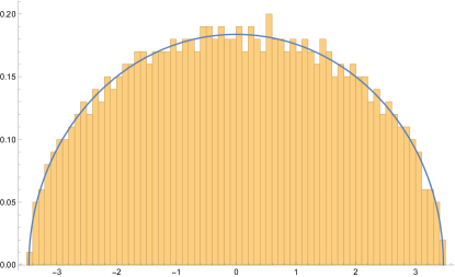
Figure 1. Density of $a+i(ab-ba)$ in the case $a$ semicircle and $b$ Bernoulli together with matrix approximation.

7.4. An example with three variables

Next we consider the example of product $XZYZX$. The linearization matrix for $(1-z^{5}XZYZX)$ is given by

$$\begin{bmatrix}0&X&0&0&0\\ 0&0&Z&0&0\\ 0&0&0&Y&0\\ 0&0&0&0&Z\\ X&0&0&0&0\end{bmatrix}$$

In order to state an explicit result let us assume that $a,b,c$ are free $a,b$ have distribution $1/2\left(\delta_{-1}+\delta_{1}\right)$ and $c$ has distribution $1/2\left(\delta_{0}+\delta_{2}\right)$. The distribution of $acbca$ is the same as free multiplicative convolution of $c$ and $b$, however the conditional expectation on $a,b$ is a non-trivial problem. We omit the lengthy calculation wich results in the expression

$$\mathbb{E}_{a,b}\left[(1-z^{5}acbca)^{-1}\right]\\ =1-a\left(\left(2z^{5}\left(8z^{10}+\gamma\right)-\left(b\left(\gamma-4\right)z^{5}+4z^{10}+2\right)^{-1}\left(-8z^{10}+\gamma\right)\right)^{-1}\right.\\ \left.\left(b\left(\gamma-4\right)z^{5}+4z^{10}+2\right)\left(\left(-8z^{10}+\gamma\right)a+4az^{10}\right)+a\right)$$

where $\gamma=\sqrt{1-16z^{10}}+1$ for the conditional expectation.

7.5. A rational example

Non–commutative rational functions have linearizations just like polynomials, (see, e.g., [16] for excellent discussion about relations between linearizations and questions in free probability) and consequently our method is not restricted to polynomials but also allows to compute conditional expectations and distributions of non–commutative rational functions in free random variables. Let us illustrate this with the concrete example of a rational function $r(a,b)=a(I-a-b)^{-1}a$ which will show that nevertheless certain technical issues arise. First we must put conditions on the distributions of $a$ and $b$ in order for $I-a-b$ to be invertible. Next we compute the conditional expectation of $(1-zr(a,b))^{-1}$ onto $a$ and $b$ and then integrate the latter in order to determine the distribution of $a(I-a-b)^{-1}a$. Using the method described in Section B we obtain the linearization

$$\left(1-zX(1-X-Y)^{-1}X\right)^{-1}=u^{t}(I_{2}-L)^{-1}v$$

where $L=C_{X}X+C_{Y}Y$ with

$$C_{X}=\begin{bmatrix}0&z\\ 1&1\end{bmatrix}\quad C_{Y}=\begin{bmatrix}0&0\\ 0&1\end{bmatrix}$$

and $u=v=(1,0)^{t}$.

Let us record some observations here. In order to be able to use iteration from Lemma 6.13 we need to start with correct constant terms $F_{X}=\beta_{1}(X)I$ and $F_{Y}=\beta_{1}(Y)I$, however there is a catch: The constant term in $F_{X}(z)=\beta^{\delta}_{X}(X(1-L)^{-1})$ is not equal to $\beta_{1}(X)$, as there are more entries which do not depend on $z$. Therefore in order to be able to distinguish the correct solution, which comes from Lemma 6.13 we introduce an extra parameter $s\in{\mathbb{C}}$ and we consider $F_{X}(s,z)=\beta^{\delta}_{X}(X(1-sL)^{-1})$, Then our iteration gives the unique solution to the system of equations for matrices $F_{X},F_{Y}$ whose entries are power series in $s$. When we want to evaluate our conditional expectation in $X=a$ and $Y=b$, of some free variables $a,b\in\mathcal{M}$, we have to make sure that for $\mu$ being their joint distribution functional $\beta^{\delta}_{X}\left(X(1-sL)^{-1}\right)$ is analytic at $s=1$. The following rough estimate will ensure this.

Denote by $W$ the set of monomials with coefficient $1$ in ${\mathbb{C}}\langle X,Y\rangle$, i.e., $W=\{X,Y,XY,\ldots\}$. For $w=Z_{1}\cdots Z_{n}\in W$ we denote $C_{w}=C_{Z_{1}}\cdots C_{Z_{n}}$. We will also use notation $|w|$ for the number of letters in $w$ and $|w|_{X},|w|_{Y}$ for the number of appearances of $X$ and $Y$ respectively in $w$, of course $|w|=|w|_{X}+|w|_{Y}$. We have

$$\beta^{\delta}_{X}\left(X(1-sL)^{-1}\right)=\sum_{w\in W}s^{|w|}\beta^{\delta}_{X}(Xw)C_{w}.$$

A standard estimate for Boolean cumulant gives $|\beta^{\delta}_{X}(Xw)|\leq 2^{|w|+1}||a||^{|w|_{x}+1}||b||^{|w|_{y}}$. Moreover it is easy to verify that $||C_{X}||^{2}\leq 2+|z|^{2}$ and $||C_{Y}||=1$. Thus we have

$$|\beta^{\delta}_{X}\left(X(1-sL)^{-1}\right)| \leq\sum_{w\in W}s^{|w|}|\beta^{\delta}_{X}(Xw)|\cdot||C_{w}||$$

$$\leq\sum_{w\in W}s^{|w|}|2^{|w|+1}||a||^{|w|_{x}+1}||b||^{|w|_{Y}}|||C_{X}||^{|w|_{X}+1}\cdot||C_{Y}||^{|w|_{Y}}$$

$$=2||a||\left(1-2s(||a||\cdot||C_{X}||+||b||\cdot||C_{Y}||)\right)^{-1}.$$

The last equality holds whenever $2s(||a||\cdot||C_{X}||+||b||\cdot||C_{Y}||<1$ and a sufficient condition for this inequality is $2s(||a||\sqrt{2+|z|^{2}}+||b||)<1$. Since we need to evaluate $\beta^{\delta}_{X}\left(X(1-sL)^{-1}\right)$ at $s=1$, our method applies for $||a||,||b||$ and $z$ such that $2(||a||\sqrt{2+|z|^{2}}+||b||)<1$.

We will apply this to $a,b$ having Bernoulli distributions $\tfrac{1}{2}\left(\delta_{-\alpha}+\delta_{-\alpha}\right)$, where in order to have a non-empty range of $z$ we need to assume $\alpha<\tfrac{\sqrt{2}-1}{2}$. So let us consider the example $\alpha=1/8$.

Before evaluation in $X=a$ and $Y=b$, taking $s=1$ we obtain

$$\operatorname{\mathbb{E}}_{X}\left[\left(1-zX(1-X-Y)^{-1}X\right)^{-1}\right]=\frac{1-fy_{22}-X}{1-fy_{22}-X-Xz(fy_{21}+X)}$$

Solving the system of equations for $F_{X}$ and $F_{Y}$, and next evaluating at the resulting expression in $X=a$, $Y=b$ as described above we get

$$\operatorname{\mathbb{E}}_{a}\left[\left(1-za(1-a-b)^{-1}a\right)^{-1}\right]=\frac{1-2a+\alpha^{2}z+\sqrt{\left(\alpha^{2}z-1\right)^{2}-4\alpha^{2}}}{1-2a(az+1)+\sqrt{\alpha^{4}z^{2}-2\alpha^{2}(z+2)+1}+\alpha^{2}z}.$$

Integrating with respect to the distribution of $a$ we get the moment transform

$$M_{a(1-a-b)^{-1}a}(z)=1+\frac{\alpha^{2}z}{\sqrt{\left(\alpha^{2}z-1\right)^{2}-4\alpha^{2}}}.$$

Taking $\alpha=1/8$ we can calculate the density and compare it with the matrix approximation shown in Figure 2.

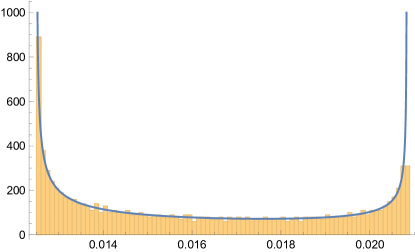
Figure 2. Density of $a(1-a-b)^{-1}a$ for $a,b$ with distribution $0.5(\delta_{-1/8}+\delta_{1/8}).$

together with matrix approximation.

Appendix A An algebraic approach to Boolean cumulants

In this first appendix we present purely algebraic proofs of basic facts about Boolean cumulants and implement a formal calculus on the double tensor product.

A.1. Algebraic proofs of Lemma 2.6 and Corollary 2.7

Proof of Lemma 2.6.

Induction on $n$. We compute $\varphi(a_{1}a_{2}\cdots a_{n})$ in two ways. First consider $a_{p}a_{p+1}$ as one factor and apply recurrence (2.2), splitting the sum into two at the entry $a_{p}a_{p+1}$.

(A.1) $$\varphi(a_{1}a_{2}\dotsm(a_{p}a_{p+1})a_{p+2}\cdots a_{n})\\ \begin{aligned} &=\begin{multlined}\sum_{k=1}^{p-1}\beta_{k}(a_{1},a_{2},\dots,a_{k})\,\varphi(a_{k+1}a_{k+2}\cdots a_{n})\\ +\sum_{k=p+1}^{n-1}\beta_{k-1}(a_{1},a_{2},\dots,a_{p}a_{p+1},a_{p+2},\dots,a_{k})\,\varphi(a_{k+1}a_{k+2}\cdots a_{n})\\ +\beta_{n-1}(a_{1},a_{2},\dots,a_{p}a_{p+1},a_{p+2},\dots,a_{n})\end{multlined}\sum_{k=1}^{p-1}\beta_{k}(a_{1},a_{2},\dots,a_{k})\,\varphi(a_{k+1}a_{k+2}\cdots a_{n})\\ +\sum_{k=p+1}^{n-1}\beta_{k-1}(a_{1},a_{2},\dots,a_{p}a_{p+1},a_{p+2},\dots,a_{k})\,\varphi(a_{k+1}a_{k+2}\cdots a_{n})\\ +\beta_{n-1}(a_{1},a_{2},\dots,a_{p}a_{p+1},a_{p+2},\dots,a_{n})\end{aligned}$$

The left hand side is unchanged if we consider $a_{p}$ and $a_{p+1}$ as separate factors. We apply recurrence (2.2), (artificially) splitting the sum at the entry $a_{p}$.

(A.2) $$\varphi(a_{1}a_{2}\dotsm a_{p}a_{p+1}a_{p+2}\cdots a_{n})\\ \begin{aligned} &=\begin{multlined}\sum_{k=1}^{p-1}\beta_{k}(a_{1},a_{2},\dots,a_{k})\,\varphi(a_{k+1}a_{k+2}\cdots a_{n})+\beta_{p}(a_{1},a_{2},\dots,a_{p})\,\varphi(a_{p+1}a_{p+2}\cdots a_{n})\\ +\sum_{k=p+1}^{n-1}\beta_{k}(a_{1},a_{2},\dots,a_{k})\,\varphi(a_{k+1}a_{k+2}\cdots a_{n})+\beta_{n}(a_{1},a_{2},\dots,a_{n})\end{multlined}\sum_{k=1}^{p-1}\beta_{k}(a_{1},a_{2},\dots,a_{k})\,\varphi(a_{k+1}a_{k+2}\cdots a_{n})+\beta_{p}(a_{1},a_{2},\dots,a_{p})\,\varphi(a_{p+1}a_{p+2}\cdots a_{n})\\ +\sum_{k=p+1}^{n-1}\beta_{k}(a_{1},a_{2},\dots,a_{k})\,\varphi(a_{k+1}a_{k+2}\cdots a_{n})+\beta_{n}(a_{1},a_{2},\dots,a_{n})\end{aligned}$$

The first part is the same in both expressions. By induction hypothesis, the second part of (A.1) can be replaced by

$$\sum_{k=p+1}^{n-1}\beta_{k-1}(a_{1},a_{2},\dots,a_{p}a_{p+1},a_{p+2},\dots,a_{k})\,\varphi(a_{k+1}a_{k+2}\cdots a_{n})\\ =\sum_{k=p+1}^{n-1}(\beta_{p}(a_{1},a_{2},\dots,a_{p})\beta_{k-p}(a_{p+1},a_{p+2},\dots,a_{k})+\beta_{k}(a_{1},a_{2},\dots,a_{k}))\,\varphi(a_{k+1}a_{k+2}\cdots a_{n}).$$

On the other hand, applying recurrence (2.2) to the second part of (A.2) we obtain

$$\beta_{p}(a_{1},a_{2},\dots,a_{p})\,\varphi(a_{p+1}a_{p+2}\cdots a_{n})\\ =\beta_{p}(a_{1},a_{2},\dots,a_{p})\sum_{k=p+1}^{n-1}\beta_{k-p}(a_{p+1},a_{p+2},\dots,a_{k})\,\varphi(a_{k+1}a_{k+2}\cdots a_{n})\\ +\beta_{p}(a_{1},a_{2},\dots,a_{p})\beta_{n-p}(a_{p+1},a_{p+2},\dots,a_{n})$$

Finally canceling equal terms from (A.1) and (A.2) we arrive at (2.8). ∎

Proof of Corollary 2.7.

By induction on the number $r$ of multiplication signs. For $r=0$ there is nothing to prove; for $r=1$ this is Lemma 2.6.

Assume that the formula holds up to $r-1$ multiplication signs and consider a Boolean cumulant of the form (2.9) with $r$ multiplication signs, i.e., $r=n-m-1$. Now apply (2.8) to remove the first multiplication

$$\beta_{m+1}(a_{1}a_{2}\cdots a_{d_{1}},a_{d_{1}+1}a_{d_{1}+2}\cdots a_{d_{2}},\ldots,a_{d_{m}+1}a_{d_{m}+2}\cdots a_{n})\\ =\beta_{1}(a_{1})\beta_{m+1}(a_{2}\cdots a_{d_{1}},a_{d_{1}+1}a_{d_{1}+2}\cdots a_{d_{2}},\ldots,a_{d_{m}+1}a_{d_{m}+2}\cdots a_{n})\\ +\beta_{m+2}(a_{1},a_{2}\cdots a_{d_{1}},a_{d_{1}+1}a_{d_{1}+2}\cdots a_{d_{2}},\ldots,a_{d_{m}+1}a_{d_{m}+2}\cdots a_{n}).$$

In both terms there are now $r-1$ multiplications and the induction hypothesis can be applied to obtain (2.9). ∎

A.2. Boolean cumulants via tensor algebras

For a vector space $V$ denote by $\operatorname{\mathcal{T}}(V)=\bigoplus_{n\geq 0}V^{\otimes n}$ its tensor algebra and $\operatorname{\overline{\mathcal{T}}}(V)=\bigoplus_{n>0}V^{\otimes n}$ its augmentation ideal, i.e., $\operatorname{\overline{\mathcal{T}}}(V)=\ker\epsilon$, where $\epsilon$ is the projection onto ${\mathbb{C}}=V^{\otimes 0}$ called the counit. In order to distinguish different levels in the hierarchy of tensors we will denote the multiplication in $\operatorname{\mathcal{T}}(V)$ by the symbol and thus elementary tensors are written $a_{1}\oocirc a_{2}\oocirc\dotsm\oocirc a_{n}$. The “outer” tensor on the double tensor algebra $\operatorname{\mathcal{T}}(\operatorname{\overline{\mathcal{T}}}(V))$ is denoted by the usual symbol $\otimes$, i.e., any element of $\operatorname{\mathcal{T}}(\operatorname{\overline{\mathcal{T}}}(V))$ is a sum of simple tensors of the form

$$(a_{1}\oocirc a_{2}\oocirc\dotsm\oocirc a_{k})\otimes(b_{1}\oocirc b_{2}\oocirc\dotsm\oocirc b_{l})\otimes\dotsm\otimes(c_{1}\oocirc c_{2}\oocirc\dotsm\oocirc c_{m}).$$

The tensor algebra has the following fundamental extension property [26, Prop. 1.1.2]:

Lemma A.1.

Let $V$ be a vector space and $M$ a $\operatorname{\mathcal{T}}(V)$-bimodule. Then any linear map $f\mathrel{\mathop{\mathchar 58\relax}}V\to M$ can be extended to a derivation $\operatorname{\mathcal{T}}(f)\mathrel{\mathop{\mathchar 58\relax}}\operatorname{\mathcal{T}}(V)\to M$ by setting

$$\operatorname{\mathcal{T}}(f)(v_{1}\oocirc v_{2}\oocirc\dotsm\oocirc v_{n})=\sum_{k=1}^{n}v_{1}\oocirc v_{2}\oocirc\dotsm\oocirc v_{k-1}\oocirc f(v_{k})\oocirc v_{k+1}\oocirc v_{k+2}\oocirc\dotsm\oocirc v_{n}$$

In the following the underlying vector space will always be an algebra $V=\mathcal{A}$, whose multiplication will be denoted as usual by $ab$ or $a\cdot b$.

For example, let $\mathcal{A}$ be the free algebra and $\operatorname{\bar{\Delta}_{d}}\mathrel{\mathop{\mathchar 58\relax}}\mathcal{A}\to\mathcal{A}\otimes\mathcal{A}\subseteq\operatorname{\overline{\mathcal{T}}}(\mathcal{A})\otimes\operatorname{\overline{\mathcal{T}}}(\mathcal{A})$ the reduced deconcatenation coproduct

$$\operatorname{\bar{\Delta}_{d}}(a_{1}a_{2}\dotsm a_{n})=\sum_{k=1}^{n-1}a_{1}a_{2}\dotsm a_{k}\otimes a_{k+1}\dotsm a_{n};$$

let further

$$\operatorname{\tilde{\Delta}_{d}}(a_{1}a_{2}\dotsm a_{n})=a_{1}\oocirc a_{2}\oocirc\dotsm\oocirc a_{n}\in\operatorname{\mathcal{T}}(\mathcal{A})$$

the full deconcatenation, i.e., $\operatorname{\tilde{\Delta}_{d}}(w_{1}w_{2})=\operatorname{\tilde{\Delta}_{d}}(w_{1}\oocirc w_{2})$. Then the derivation from Lemma A.1 is

$$\operatorname{\mathcal{T}}(\operatorname{\bar{\Delta}_{d}})(w_{1}\oocirc w_{2}\oocirc\dotsm\oocirc w_{n})=\sum_{k=1}^{n-1}((w_{1}\oocirc w_{2}\oocirc\dotsm\oocirc w_{k-1})\otimes 1)\oocirc\operatorname{\bar{\Delta}_{d}}(w_{k})\oocirc(1\otimes(w_{k+1}\oocirc\dotsm\oocirc w_{n}))$$

We will denote this derivation by $\operatorname{\bar{\Delta}_{d}}$ as well.

The moment and cumulant functionals are defined on $\operatorname{\overline{\mathcal{T}}}(\mathcal{A})$ via

$$\varphi(w_{1}\oocirc w_{2}\oocirc\dotsm\oocirc w_{n}) =\varphi(w_{1}w_{2}\dotsm w_{n})$$

$$\beta(w_{1}\oocirc w_{2}\oocirc\dotsm\oocirc w_{n}) =\beta_{n}(w_{1},w_{2},\dots,w_{n})$$

and the recurrence (2.2) can be reformulated with the second level deconcatenation operator $\operatorname{\bar{\Delta}_{d}}\mathrel{\mathop{\mathchar 58\relax}}\operatorname{\overline{\mathcal{T}}}(A)\to\operatorname{\overline{\mathcal{T}}}(A)\otimes\operatorname{\overline{\mathcal{T}}}(A)$ defined by

$$\operatorname{\bar{\Delta}_{d}}(w_{1}\oocirc w_{2}\oocirc\dotsm\oocirc w_{n})=\sum_{k=1}^{n-1}w_{1}\oocirc w_{2}\oocirc\dotsm\oocirc w_{k}\otimes w_{k+1}\oocirc w_{k+2}\oocirc\dotsm\oocirc w_{n}$$

as follows:

$$\varphi(w_{1}\oocirc w_{2}\oocirc\dotsm\oocirc w_{n})=\beta(w_{1}\oocirc w_{2}\oocirc\dotsm\oocirc w_{n})+(\beta\otimes\varphi)\operatorname{\bar{\Delta}_{d}}(w_{1}\oocirc w_{2}\oocirc\dotsm\oocirc w_{n})$$

On the other hand, if we define the full Boolean cumulant $\beta^{\delta}(w)=\beta(\operatorname{\tilde{\Delta}_{d}}(w))$, i.e.

$$\beta^{\delta}(a_{1}a_{2}\dotsm a_{n})=\beta(a_{1}\oocirc a_{2}\oocirc\dotsm\oocirc a_{n})=\beta_{n}(a_{1},a_{2},\dots,a_{n})$$

and extend it to $\operatorname{\overline{\mathcal{T}}}(\mathcal{A})$ via

$$\beta^{\delta}(w_{1}\oocirc w_{2}\oocirc\dotsm\oocirc w_{n}) =\beta^{\delta}(w_{1}w_{2}\dotsm w_{n})$$

$$=\beta(\operatorname{\tilde{\Delta}_{d}}(w_{1})\oocirc\operatorname{\tilde{\Delta}_{d}}(w_{2})\oocirc\dotsm\oocirc\operatorname{\tilde{\Delta}_{d}}(w_{n}))$$

then the full Boolean cumulants satisfy the corresponding recurrence

$$\varphi(w)=\beta^{\delta}(w)+(\beta^{\delta}\otimes\varphi)\operatorname{\bar{\Delta}_{d}}(w)$$

which we can generalize to $\operatorname{\overline{\mathcal{T}}}(\mathcal{A})$. In order to formulate it, we introduce some further notation.

Definition A.2.

An interval partition is a partition whose blocks are intervals. The interval partitions $\operatorname{\mathrm{Int}}(\{1,2,\dots,n\})$ are thus in bijection with compositions $\operatorname{\mathcal{C}}(n)=\{(k_{1},k_{2},\dots,k_{m})\mid k_{1}+k_{2}+\dotsm k_{m}=n\}$. The bijection maps an interval partition $\pi\in\operatorname{\mathrm{Int}}(n)$ to the sequence of block lengths (in their natural order). We denote this bijection by $C\mathrel{\mathop{\mathchar 58\relax}}\operatorname{\mathrm{Int}}(n)\to\operatorname{\mathcal{C}}(n)$. A composition $\lambda=(k_{1},k_{2},\dots,k_{m})\in\operatorname{\mathcal{C}}(n)$ is uniquely determined by its partial sums, called descents

$$\operatorname{\mathcal{D}}(\lambda)=\{k_{1},k_{1}+k_{2},\dots,k_{1}+k_{2}+\dotsm+k_{m-1}\}\subseteq\{1,2,\dots,n-1\}$$

and thus the compositions of order $n$ are in bijection with the Boolean lattice of order $n-1$, The descents of an interval partition are the descents of the corresponding composition $\operatorname{\mathcal{D}}(\pi)=\operatorname{\mathcal{D}}(C(\pi))$. This bijection is a poset anti-isomorphism and $\pi\leq\rho$ if and only if $\operatorname{\mathcal{D}}(\rho)\supseteq\operatorname{\mathcal{D}}(\pi)$. In particular, $\operatorname{\mathcal{D}}(\pi\vee\rho)=\operatorname{\mathcal{D}}(\pi)\cap\operatorname{\mathcal{D}}(\rho)$.

Proposition A.3.

$$\beta(w_{1}\oocirc w_{2}\oocirc\dotsm\oocirc w_{n})=\beta^{\delta}(w_{1}\oocirc w_{2}\oocirc\dotsm\oocirc w_{n})+(\beta^{\delta}\otimes\beta)\circ\operatorname{\bar{\Delta}_{d}}(w_{1}\oocirc w_{2}\oocirc\dotsm\oocirc w_{n})$$

Proof.

Let $k_{i}=\ell(w_{i})$ be the lengths of the words and $\rho=\{I_{1},I_{2},\dots,I_{m}\}\in\operatorname{\mathrm{Int}}(n)$ the induced interval partition, i.e., $\mathinner{\!\left\lvert I_{j}\right\rvert}=k_{j}$ and $C(\rho)=(k_{1},k_{2},\dots,k_{m})$ with descent set $\operatorname{\mathcal{D}}(\rho)=\{r_{1},r_{2},\dots,r_{m-1}\}$ where $r_{0}=d_{0}(\rho)=0$, $r_{1}=d_{1}(\rho)=k_{1}$, $r_{2}=d_{2}(\rho)=k_{1}+k_{2}$, etc. Then if $w_{i}=a_{r_{i-1}+1}a_{r_{i-1}+2}\dotsm a_{r_{i}}$ the product formula (2.7) can be rewritten in terms of descents as

$$\beta_{m}(a_{1}a_{2}\cdots a_{r_{1}},a_{r_{1}+1}\dotsm a_{r_{2}},\ldots,a_{r_{m-1}+1}\cdots a_{n})\\ \begin{aligned} &=\sum_{\begin{subarray}{c}\pi\in\operatorname{\mathrm{Int}}(n)\\ \operatorname{\mathcal{D}}(\pi)\cap\operatorname{\mathcal{D}}(\rho)=\emptyset\end{subarray}}\beta_{\pi}(a_{1},\ldots,a_{n})\\ &=\beta_{n}(a_{1},a_{2},\dots,a_{n})+\sum_{s=1}^{m}\sum_{\begin{subarray}{c}\pi\in\operatorname{\mathrm{Int}}(n)\setminus\{1_{n}\}\\ \operatorname{\mathcal{D}}(\pi)\cap\operatorname{\mathcal{D}}(\rho)=\emptyset\\ d_{1}(\pi)\in I_{s}\end{subarray}}\beta_{\pi}(a_{1},\ldots,a_{n})\end{aligned}$$

where we split off the term corresponding to $\pi=1_{n}$ (i.e., $\operatorname{\mathcal{D}}(\pi)=\emptyset$) and regroup the remaining terms according to the location of the first descent $d_{1}(\pi)$. Fix $1\leq s\leq m$ and assume that $d=d_{1}(\pi)\in I_{s}$. Then the first block of $\pi$ is $B_{1}=\{1,2,\dots,d_{1}\}$ and $\pi=\{B_{1}\}\cup\pi^{\prime}$ with $\pi^{\prime}=\pi|_{[d+1,n]}\in\operatorname{\mathrm{Int}}[d+1,n]$ and $\operatorname{\mathcal{D}}(\pi^{\prime})\cap\operatorname{\mathcal{D}}(\rho^{\prime})=\emptyset$ where $\rho^{\prime}=\rho|_{[d+1,n]}$. Now by assumption $r_{s-1}<d<r_{s}$ and thus

$$\sum_{\begin{subarray}{c}\pi\in\operatorname{\mathrm{Int}}(n)\setminus\{1_{n}\}\\ \operatorname{\mathcal{D}}(\pi)\cap\operatorname{\mathcal{D}}(\rho)=\emptyset\\ d_{1}(\pi)\in I_{s}\end{subarray}}\beta_{\pi}(a_{1},\ldots,a_{n})\\ \begin{aligned} &=\sum_{d=r_{s-1}+1}^{r_{s}-1}\beta_{d}(a_{1},a_{2},\dots,a_{d})\sum_{\begin{subarray}{c}\pi^{\prime}\in\operatorname{\mathrm{Int}}([d+1,n])\\ \operatorname{\mathcal{D}}(\pi^{\prime})\cap\operatorname{\mathcal{D}}(\rho^{\prime})=\emptyset\end{subarray}}\beta_{\pi^{\prime}}(a_{d+1},a_{d+2},\ldots,a_{n})\\ &=\sum_{d=r_{s-1}+1}^{r_{s}-1}\beta_{d}(a_{1},a_{2},\dots,a_{d})\,\beta_{m-s+1}(a_{d+1}a_{d+2}\dotsm a_{r_{s}},w_{s+1},w_{s+2},\dots,w_{n})\\ &=(\beta^{\delta}\otimes\beta)((w_{1}\oocirc w_{2}\oocirc\dotsm\oocirc w_{s-1}\otimes 1)(\operatorname{\bar{\Delta}_{d}}w_{s})(1\otimes(w_{s+1}\oocirc w_{s+2}\oocirc\dotsm\oocirc w_{m})))\end{aligned}$$

∎

Remark A.4.

Although freeness implies property $(CAC)$ (Lemma 3.5) and thus $\beta^{\delta}(w_{1}\oocirc w_{2}\oocirc\dotsm\oocirc w_{n})=0$ if $w_{1}$ begins with $X$ and $w_{n}$ ends in $Y$, it is important to keep in mind that this is not necessarily true for $\beta{}(w_{1}\oocirc w_{2}\oocirc\dotsm\oocirc w_{n})$.

Example A.5 (Cumulants of products).

Let us apply Proposition A.3 to

$$\Psi=\sum_{n=0}^{\infty}(XY)^{\oocirc n}z^{2n}$$

to compute the cumulant generating function

$$B(z)=\beta(\Psi)=\sum_{n=0}^{\infty}\beta_{n}(XY)z^{2n}.$$

From this we can then obtain the moment generating function

$$M(z)=\frac{1}{1-B(z)}.$$

Applying the Leibniz rule to the identity $\Psi\oocirc(1-z^{2}XY)=1$ we obtain (2.17)

$$\operatorname{\bar{\Delta}_{d}}(\Psi)=(\Psi\oocirc X)\otimes(Y\oocirc\Psi)z^{2}.$$

Now by Proposition A.3 we have

$$\beta(\Psi) =\beta^{\delta}(\Psi)+\beta^{\delta}(\Psi\oocirc X)\beta(Y\oocirc\Psi)z^{2}$$

and similarly

$$\operatorname{\bar{\Delta}_{d}}(Y\oocirc\Psi) =(Y\otimes 1)\oocirc\operatorname{\bar{\Delta}_{d}}(\Psi)$$

$$=(Y\oocirc\Psi\oocirc X)\otimes(Y\oocirc\Psi)z^{2}$$

$$\beta(Y\oocirc\Psi) =\beta^{\delta}(Y\oocirc\Psi)+\beta^{\delta}(Y\oocirc\Psi\oocirc X)\beta(Y\oocirc\Psi)z^{2}.$$

Consequently,

$$\beta(Y\oocirc\Psi) =\frac{\beta^{\delta}(Y\oocirc\Psi)}{1-\beta^{\delta}(y\oocirc\Psi\oocirc X)z^{2}}$$

$$\beta(\Psi) =\beta^{\delta}(\Psi)+\frac{\beta^{\delta}(\Psi\oocirc X)\,\beta^{\delta}(Y\oocirc\Psi)z^{2}}{1-\beta^{\delta}(Y\oocirc\Psi\oocirc X)z^{2}}$$

where

$$\beta^{\delta}(\Psi\oocirc X) =\sum_{n=0}^{\infty}\beta_{2n+1}(X,Y,X,Y,\dots,X)z^{2n}$$

$$\beta^{\delta}(Y\oocirc\Psi) =\sum_{n=0}^{\infty}\beta_{2n+1}(Y,X,Y,X,\dots,Y)z^{2n}$$

If we assume $x$ and $y$ free then we infer from the resolvent identity

$$\Psi=1+z^{2}XY\Psi$$

that $\beta^{\delta}(\Psi)=1$ and $\beta^{\delta}(Y\oocirc\Psi\oocirc X)=0$ and thus

$$\beta(\Psi)-1=\beta^{\delta}(\Psi\oocirc X)\,\beta^{\delta}(Y\oocirc\Psi)$$

Thus

$$B(z)=\beta(\Psi)=1+z\beta^{\delta}_{X}(\Psi X)\beta^{\delta}_{Y}(Y\Psi)$$

and finally

$$zB(z)=z+\omega_{1}(z)\,\omega_{2}(z)$$

which reproduces [3, Theorem 3.2 (3)] and [11, (10)].

Appendix B Rational series and linearizations

The non–commutative free field and in particular non–commutative rational functions have seen many applications in free probability recently [16]. The main tool for their study are linearizations. For technical reasons we restrict our study to regular rational functions, i.e., rational functions which can be represented as formal power series. These form a subalgebra of ${\mathbb{C}}\langle\!\langle{\mathcal{X}}\rangle\!\rangle$ and can be characterized in several ways [6].

Definition B.1.

For a series $S\in{\mathbb{C}}\langle\!\langle{\mathcal{X}}\rangle\!\rangle$ we denote the extraction of coefficients by $\langle S,w\rangle$, i.e.,

$$S=\sum_{w\in{\mathcal{X}}^{*}}\langle S,w\rangle\,w.$$

A series $S\in{\mathbb{C}}\langle\!\langle{\mathcal{X}}\rangle\!\rangle$ is called proper if it has no constant term, i.e., $\langle S,1\rangle=0$. Proper series have a quasi-inverse

$$S^{+}=\sum_{k=1}^{\infty}S^{k}\in{\mathbb{C}}\langle\!\langle{\mathcal{X}}\rangle\!\rangle.$$

$Q=S^{+}$ is the unique solution of the equation

$$Q=S+QS.$$

The algebra of rational series is the smallest subalgebra of ${\mathbb{C}}\langle\!\langle{\mathcal{X}}\rangle\!\rangle$ which contains all quasi-inverses of its proper elements. This implies that for any element $S$ without constant term the element $1-S$ is invertible and its inverse is given by the geometric series

$$(1-S)^{-1}=\sum_{k=0}^{\infty}S^{k}\in{\mathbb{C}}\langle\!\langle{\mathcal{X}}\rangle\!\rangle$$

and therefore rational.

A series $S\in{\mathbb{C}}\langle\!\langle{\mathcal{X}}\rangle\!\rangle$ is called recognizable if there exists a matrix representation of the free monoid, i.e., a multiplicative map $\rho\mathrel{\mathop{\mathchar 58\relax}}{\mathcal{X}}^{*}\to M_{n}({\mathbb{C}})$, and vectors $u,v\in{\mathbb{C}}^{n}$ such that the coefficients of $S$ are given by

$$\langle S,w\rangle=u^{t}\rho(w)v.$$

Here the representation $\rho$ is uniquely determined by the matrices $M_{x}=\rho(x)$ for $x\in{\mathcal{X}}$. Indeed, $\rho(x_{1}x_{2}\dotsm x_{k})=M_{x_{1}}M_{x_{2}}\dotsm M_{x_{k}}$ and thus a recognizable series has a linearization

$$S=u^{t}\Bigl{(}\sum_{w\in{\mathcal{X}}^{*}}\rho(w)\,w\Bigr{)}v=u^{t}\Bigl{(}1-\sum_{x\in{\mathcal{X}}}M_{x}x\Bigr{)}^{-1}v.$$

Conversely, any series which is given by a linearization is recognizable.

Definition B.2.

For a letter $x\in{\mathcal{X}}$ denote by $L_{x}$ the left annihilation operator on ${\mathbb{C}}\langle\!\langle{\mathcal{X}}\rangle\!\rangle$, i.e., for a word $w\in{\mathcal{X}}^{*}$ set

$$L_{x}w=\begin{cases}w^{\prime}&\text{if $w=xw^{\prime}$}\\ 0&\text{otherwise}\end{cases}$$

and extend this operator linearly to ${\mathbb{C}}\langle\!\langle{\mathcal{X}}\rangle\!\rangle$. For a word $w=x_{1}x_{2}\dotsm x_{n}\in{\mathcal{X}}^{*}$ we denote by $L_{w}=L_{x_{n}}L_{x_{n-1}}\dotsm L_{x_{1}}$ the composition of the annihilation operators.

A subspace $U\subseteq{\mathbb{C}}\langle\!\langle{\mathcal{X}}\rangle\!\rangle$ is called stable if it is invariant under $L_{x}$ for all $x\in{\mathcal{X}}$.

Remark B.3.

With this notation the coefficients of a series are given by

(B.1) $$\langle S,w\rangle=\langle L_{w}S,1\rangle$$

One of the main results of the theory of rational series is the following

Theorem B.4 ([6]).

For a series $S\in{\mathbb{C}}\langle\!\langle{\mathcal{X}}\rangle\!\rangle$ the following are equivalent,

1. $S$ is rational.

2. $S$ is recognizable.

3. $S$ has a linearization.

4. There is a finite dimensional stable subspace of ${\mathbb{C}}\langle\!\langle{\mathcal{X}}\rangle\!\rangle$ containing $S$.

The last statement gives rise to an algorithm key to compute linearizations of rational series.

Algorithm B.5.

Assume our series $S$ is contained in a finite dimensional stable subspace spanned by a basis $(S_{1},S_{2},\dots,S_{N})\subseteq{\mathbb{C}}\langle\!\langle{\mathcal{X}}\rangle\!\rangle$, say $S=\sum u_{i}S_{i}$.

1. Since the subspace is stable, for any $X\in{\mathcal{X}}$ we can express

   $$L_{x}S_{i}=\sum\alpha_{ij}(x)S_{j}.$$

2. Collect these coefficients in a matrix $A_{x}=\left[\alpha_{ij}(x)\right]$.

3. Then for a word $w\in{\mathcal{X}}^{*}$ after iteration we obtain

   $$L_{w}S_{i}=\sum_{j}(M_{w})_{ij}S_{j}.$$

4. From (B.1) we infer $\langle S_{i},w\rangle=\langle L_{w}S,1\rangle=(M_{w}v)_{i}$.

5. Finally $\langle S,w\rangle=u^{t}M_{w}v$ for every $w\in\mathcal{X}^{*}$, i.e.,

   $$S=u^{t}\Bigl{(}I_{N}-\sum_{x\in\mathcal{X}}M_{x}x\Bigr{)}^{-1}v.$$

To illustrate this let us start with polynomials which are clearly rational. Let $w\in{\mathcal{X}}^{*}$ be a word. A word $w^{\prime\prime}\in{\mathcal{X}}^{*}$ is a right suffix of $w$ if there exists a word $w^{\prime}\in{\mathcal{X}}^{*}$ such that $w=w^{\prime}w^{\prime\prime}$. Equivalently, $w^{\prime\prime}$ can be obtained from $w$ by applying the left annihilation operator $L_{w^{\prime}}$.

Let now $P\in{\mathbb{C}}\langle{\mathcal{X}}\rangle$ be a polynomial. If we successively apply annihilation operators $L_{X}$, $X\in{\mathcal{X}}$ we obtain elements contained in the span of all right suffixes of the monomials occurring in $P$ (including the empty word $1$). Clearly the span of $P$ and all its right suffixes is stable and thus can be used to obtain a linearization for $P$.

From this basis we can immediately construct a basis of a stable subspace containing $\Psi=(1-z^{m}P)^{-1}$ and construct a linearization of the latter, where $m=\deg(P)$, i.e., the length of the longest monomial in $P$. Indeed let $\{S_{1}=P,S_{2},\dots,S_{r}=1\}$ be a basis consisting of $P$ and the right suffixes of $P$ spanning a stable invariant subspace for $P$. Now we use the resolvent identity

$$\Psi=(1-z^{m}P)^{-1}=1+z^{m}P\Psi$$

to obtain $L_{x}\Psi=z^{m}(L_{x}P)\Psi$ and thus $\{\Psi,z^{m_{2}}S_{2}\Psi,\dots,z^{m_{r-1}}S_{r-1}\Psi\}$ spans a stable subspace containing $\Psi$, where $m_{i}=\deg S_{i}$. Moreover $\langle S_{i}\Psi,1\rangle=0$ for $i=2,\dots,r-1$ and thus we can set $u=v=e_{1}$. The inclusion of the factor $z^{m_{i}}$ ensures that our linearization has the form $\Psi=u^{t}(I-zL)^{-1}v$, where the entries of $L$ are polynomials in $z$ and thus has a formal power series expansion around zero, which is essential in the Section 6.

Example B.6.

Consider $P(X,Y)=X+XYX$, then we are looking for a linearization of $\Psi=(1-z^{3}P)^{-1}$. We have $\Psi=1+z^{3}P\Psi$ and thus we have

$$S_{1} =\Psi,L_{X}\Psi=z^{3}\Psi+z^{3}YX\Psi=z^{3}S_{1}+zS_{2},$$

where $S_{2}=z^{2}YX\Psi$. Of course $L_{Y}S_{1}=0$. Next $L_{X}S_{2}=0$ and $L_{Y}S_{2}=z^{2}X\Psi=zS_{3}$. Finally $L_{X}S_{3}=z\Psi=zS_{1}$ and $L_{Y}S_{3}=0$. Hence we obtain $\Psi=u^{t}(1-zL)^{-1}v$ with

$$zL=\begin{bmatrix}z^{3}&z&0\\ 0&0&0\\ z&0&0\end{bmatrix}X+\begin{bmatrix}0&0&0\\ 0&0&z\\ 0&0&0\end{bmatrix}Y.$$

Remark B.7.

Another way to obtain a linearization of $\Psi=(1-z^{m}P)^{-1}$ for a polynomial P is to directly follow the multiplication structure. Let us describe this with an example, occasionally we will use this linearization instead of the one described above.

Consider the non–commutative polynomial $XYX+YXY$ and the corresponding polynomial with numbered variables$X_{1}Y_{1}X_{2}+Y_{2}X_{3}Y_{3}$. When we look at powers of this polynomial, we see that:

• $X_{1}$ is always followed by $Y_{1}$,

• $X_{2}$ is followed by $X_{1}$ or $Y_{2}$,

• $Y_{1}$ is followed by $X_{1}$ or $Y_{2}$,

• $Y_{2}$ is always followed by $X_{2}$.

This can be represented graphically as an automaton, see Figure 3.

Figure 3. Multiplication for $X_{1}Y_{1}X_{2}+Y_{2}X_{3}Y_{3}$.

Let us name all variables in the considered polynomial $Z_{1},Z_{2},\ldots,Z_{n}$, where $n$ is the total number of variables in the polynomial. The polynomial $X_{1}Y_{1}X_{2}+Y_{2}X_{3}Y_{3}$ we have $Z_{1}Z_{2}Z_{3}+Z_{4}Z_{5}Z_{6}$, we will consider a square matrix in which each row and column corresponds to one of the variables, more precisely we set $L_{i,j}=Z_{j}$ if $Z_{j}$ follows $Z_{i}$, otherwise we set $L_{i,j}=0$. We obtain the following linearization matrix (we show the labels of rows and columns)

$$L=\,\blockarray{ccccccc}&X_{1}X_{2}X_{3}Y_{1}Y_{2}Y_{3}\\ \block{l[cccccc]}X_{1}\,000Y_{1}00\\ X_{2}\,X_{1}000Y_{2}0\\ X_{3}\,00000Y_{3}\\ Y_{1}\,0X_{2}0000\\ Y_{2}\,00X_{3}000\\ Y_{3}\,X_{1}000Y_{2}0\\$$

In order to get a linearization of $(1-z^{3}(X_{1}Y_{1}X_{2}+Y_{2}X_{3}Y_{3}))^{-1}$ we look at $(1-zL)^{-1}$, it is clear that every term in expansion of $(1-z^{3}(X_{1}Y_{1}X_{2}+Y_{2}X_{3}Y_{3}))^{-1}$ starts with $X_{1}$ or $Y_{2}$, hence $u^{t}=(0,1,0,0,0,0)$ or equivalently $u^{t}=(0,0,0,0,0,1)$. On the other hand each term in $(1-z^{3}(X_{1}Y_{1}X_{2}+Y_{2}X_{3}Y_{3})^{-1}$ ends in $X_{2}$ or $Y_{3}$, hence we have to terminate with the second or sixth column of $L$, thus $v^{t}=(0,1,0,0,0,1)$. Clearly we have the equality of formal power series

$$(1-z^{3}(X_{1}Y_{1}X_{2}+Y_{2}X_{3}Y_{3}))^{-1}=u^{t}(1-zL)^{-1}v.$$

References

- [1] D. Avitzour. Free products of -algebras. Trans. Amer. Math. Soc., 271(2):423–435, 1982.
- [2] K. I. Beidar, W. S. Martindale, III, and A. V. Mikhalev. Rings with generalized identities, volume 196 of Monographs and Textbooks in Pure and Applied Mathematics. Marcel Dekker, Inc., New York, 1996.
- [3] S. T. Belinschi and H. Bercovici. A new approach to subordination results in free probability. J. Anal. Math., 101:357–365, 2007.
- [4] S. T. Belinschi, T. Mai, and R. Speicher. Analytic subordination theory of operator-valued free additive convolution and the solution of a general random matrix problem. J. Reine Angew. Math., 732:21–53, 2017.
- [5] S. T. Belinschi and A. Nica. -series and a Boolean Bercovici-Pata bijection for bounded -tuples. Adv. Math., 217(1):1–41, 2008.
- [6] J. Berstel and C. Reutenauer. Noncommutative rational series with applications, volume 137 of Encyclopedia of Mathematics and its Applications. Cambridge University Press, Cambridge, 2011.
- [7] P. Biane. Processes with free increments. Math. Z., 227(1):143–174, 1998.
- [8] A. Bose, A. Dey, and W. Ejsmont. Characterization of non-commutative free Gaussian variables. ALEA Lat. Am. J. Probab. Math. Stat., 15(2):1241–1255, 2018.
- [9] N. Bourbaki. Éléments de mathématique. Algèbre. Chapitres 1 à 3. Hermann, Paris, 1970.
- [10] G. Cébron. Free convolution operators and free Hall transform. J. Funct. Anal., 265(11):2645–2708, 2013.
- [11] G. P. Chistyakov and F. Götze. The arithmetic of distributions in free probability theory. Cent. Eur. J. Math., 9(5):997–1050, 2011.
- [12] P. Doubilet, G.-C. Rota, and R. Stanley. On the foundations of combinatorial theory. VI. The idea of generating function. pages 267–318, 1972.
- [13] K. Ebrahimi-Fard and F. Patras. Cumulants, free cumulants and half-shuffles. Proc. A., 471(2176):20140843, 18, 2015.
- [14] M. Fevrier, M. Mastnak, A. Nica, and K. Szpojankowski. Using Boolean cumulants to study multiplication and anticommutators of free random variables. Trans. Amer. Math. Soc., 373:7167–7205, 2020.
- [15] U. Haagerup and F. Larsen. Brown’s spectral distribution measure for -diagonal elements in finite von Neumann algebras. J. Funct. Anal., 176(2):331–367, 2000.
- [16] J. W. Helton, T. Mai, and R. Speicher. Applications of realizations (aka linearizations) to free probability. J. Funct. Anal., 274(1):1–79, 2018.
- [17] T. W. Hungerford. The free product of algebras. Illinois J. Math., 12:312–324, 1968.
- [18] D. Jekel and W. Liu. An operad of non-commutative independences defined by trees, 2020.
- [19] S. A. Joni and G.-C. Rota. Coalgebras and bialgebras in combinatorics. In Umbral calculus and Hopf algebras (Norman, Okla., 1978),, Contemp. Math., 6,, pages 1–47,. ,, 1982.
- [20] B. Krawczyk and R. Speicher. Combinatorics of free cumulants. J. Combin. Theory Ser. A, 90:267–292, 2000.
- [21] F. Lehner. Free cumulants and enumeration of connected partitions. European J. Combin., 23(8):1025–1031, 2002.
- [22] F. Lehner. Cumulants in noncommutative probability theory. I. Noncommutative exchangeability systems. Math. Z., 248(1):67–100, 2004. arXiv:math/0210441.
- [23] F. Lehner and K. Szpojankowski. Boolean cumulants and subordination in free probability. Random Matrices Theory Appl., 10(4):Paper No. 2150036, 46, 2021.
- [24] V. P. Leonov and A. N. Shiryaev. On a method of calculation of semi-invariants. Theor. Prob. Appl., 4:319–328, 1959.
- [25] J.-L. Loday and M. Ronco. On the structure of cofree Hopf algebras. J. Reine Angew. Math., 592:123–155, 2006.
- [26] J.-L. Loday and B. Vallette. Algebraic operads, volume 346 of Grundlehren der mathematischen Wissenschaften [Fundamental Principles of Mathematical Sciences]. Springer, Heidelberg, 2012.
- [27] T. Mai, R. Speicher, and S. Yin. The free field: zero divisors, atiyah property and realizations via unbounded operators, 2018.
- [28] J. A. Mingo and R. Speicher. Free probability and random matrices, volume 35 of Fields Institute Monographs. Springer, New York; Fields Institute for Research in Mathematical Sciences, Toronto, ON, 2017.
- [29] N. Muraki. The five independences as quasi-universal products. Infin. Dimens. Anal. Quantum Probab. Relat. Top., 5(1):113–134, 2002.
- [30] A. Nica and R. Speicher. Commutators of free random variables. Duke Math. J., 92(3):553–592, 1998.
- [31] A. Nica and R. Speicher. Lectures on the combinatorics of free probability, volume 335 of London Mathematical Society Lecture Note Series. Cambridge University Press, Cambridge, 2006.
- [32] D. Perales. On the anti-commutator of two free random variables, 2021. arXiv:2101.09444.
- [33] M. Popa. A new proof for the multiplicative property of the Boolean cumulants with applications to the operator-valued case. Colloq. Math., 117(1):81–93, 2009.
- [34] T. P. Speed. Cumulants and partition lattices. Austral. J. Statist., 25:378–388, 1983.
- [35] R. Speicher. Multiplicative functions on the lattice of noncrossing partitions and free convolution. Math. Ann., 298(4):611–628, 1994.
- [36] R. Speicher and R. Woroudi. Boolean convolution. In Free probability theory (Waterloo, ON, 1995), volume 12 of Fields Inst. Commun., pages 267–279. Amer. Math. Soc., Providence, RI, 1997.
- [37] K. Szpojankowski and J. Wesołowski. Dual Lukacs regressions for non-commutative variables. J. Funct. Anal., 266(1):36–54, 2014.
- [38] K. Szpojankowski and J. Wesołowski. Conditional expectations through Boolean cumulants and subordination – towards a better understanding of the lukacs property in free probability. ALEA, Lat. Am. J. Probab. Math. Stat, 17:253–272, 2020.
- [39] M. Takesaki. Theory of operator algebras I. Springer-Verlag, New York-Heidelberg,,, 1979.
- [40] R. H. Terwiel. Projection operator method applied to stochastic linear differential equations. Physica, 74:248–265, 1974.
- [41] V. Vasilchuk. On the asymptotic distribution of the commutator and anticommutator of random matrices. J. Math. Phys., 44(4):1882–1908, 2003.
- [42] D. Voiculescu. Symmetries of some reduced free product -algebras. In Operator algebras and their connections with topology and ergodic theory (Bucsteni, 1983), volume 1132 of Lecture Notes in Math., pages 556–588. Springer, Berlin, 1985.
- [43] D. Voiculescu. The analogues of entropy and of Fisher’s information measure in free probability theory. I. Comm. Math. Phys., 155(1):71–92, 1993.
- [44] D. Voiculescu. The analogues of entropy and of Fisher’s information measure in free probability theory. V. Noncommutative Hilbert transforms. Invent. Math., 132(1):189–227, 1998.
- [45] D. Voiculescu. The analogues of entropy and of Fisher’s information measure in free probability theory. VI. Liberation and mutual free information. Adv. Math., 146(2):101–166, 1999.
- [46] D. V. Voiculescu, K. J. Dykema, and A. Nica. Free random variables, volume 1 of CRM Monograph Series. American Mathematical Society, Providence, RI, 1992.
- [47] W. von Waldenfels. An approach to the theory of pressure broadening of spectral lines. In Probability and information theory, II, pages 19–69. Lecture Notes in Math., Vol. 296. 1973.
- [48] W. Woess. Nearest neighbour random walks on free products of discrete groups. Boll. Un. Mat. Ital. B (6), 5(3):961–982, 1986.