Community Detection with the Map Equation and Infomap:
Theory and Applications

Abstract

Real-world networks have a complex topology comprising many elements often structured into communities. Revealing these communities helps researchers uncover the organizational and functional structure of the system that the network represents. However, detecting community structures in complex networks requires selecting a community detection method among a multitude of alternatives with different network representations, community interpretations, and underlying mechanisms. This review and tutorial focuses on a popular community detection method called the map equation and its search algorithm Infomap. The map equation framework for community detection describes communities by analyzing dynamic processes on the network. Thanks to its flexibility, the map equation provides extensions that can incorporate various assumptions about network structure and dynamics. To help decide if the map equation is a suitable community detection method for a given complex system and problem at hand – and which variant to choose – we review the map equation’s theoretical framework and guide users in applying the map equation to various research problems.

I Introduction

Networks help researchers analyze complex systems by representing their intricate interactions. To simplify networks with numerous nodes and links and uncover their essential structure and dynamics, researchers have developed an array of methods to detect communities, also called modules [1, 2]. These methods vary in goals, assumptions, and interpretations, ranging from generative models representing network formation processes to flow-based approaches capturing processes on the network [3]. When choosing a method for a specific problem, users must consider their objectives, the system under study, and the available data [4]. The multitude of methods and settings can be daunting. Users often struggle to select the most suitable approach and configuration, leading to suboptimal results.

Two questions stand out when describing network communities: How did the network form? How does the network’s structure affect processes that take place on the network? While these questions are often intertwined, and community detection methods handle assumptions about the network’s formation, structure, and dynamic processes differently, we can discern two major approaches. Different generative methods address the first question, such as community embedding models [5], community-affiliation graph models [6], and stochastic block models with Bayesian inference techniques [7]. These methods assume that a latent community structure determines the link distribution. Finding an optimal partition representing the underlying structure involves applying statistical inference to fit a generative model to the network data. Addressing the second question requires shifting focus to the processes on the network that uncover how nodes share similar dynamical roles.

We refer to processes on networks as network flows. Network flows are vital for our understanding of system-wide behavior in complex systems. They transform networks from combinatorial constructs of nodes and links into integrated representations of complex systems where distant parts can influence each other. Specifically, network flows capture the interconnected dynamics of complex systems, such as when element A interacts with element B and element B interacts with element C, elements A and C indirectly affect each other.

Sometimes, these flows are observable, such as passenger flows between airports in air traffic networks. Other times, we must model the flows. For example, when we want to comprehend genetic pathways but have access only to the gene network, we can derive flows from the interactions between pairs of genes. Since network structure constrains processes on it, studying modeled flows can also reveal meaningful structures in networks without explicit flows.

Flow-based modules coarse-grain the dynamics taking place on the network. Groups of nodes where the network flows stay relatively long provide an intuitive notion of flow-based modules. In air traffic networks, flow-based modules comprise sets of airports which contain many itineraries. In gene networks with unknown genetic pathways, functional modules trap modeled network flows representing the biological processes. In networks without explicit network flows, including synthetic benchmark networks with planted community structure of a generative model, flow-based methods have nevertheless proven effective in identifying these topological communities [8, 9, 10]. Because studying flow-based communities provides essential insights about the systems they represent, reliably identifying them is critical.

While there are several flow-based community detection methods [11, 12, 13, 14], we focus on the map equation and its search algorithm Infomap [15, 16]. The map equation captures modular regularities by compressing the description of flows, capitalizing on the minimum description length principle. Applied to modular compression of network flows, the minimum description length principle states that finding the partition that enables the greatest compression of the network flows is equivalent to identifying the modules that best capture the regularities of those flows. Given a partition, the map equation calculates the lower bound for the per-step description length of a random walk on the given network. Thanks to the map equation’s foundation in information theory and stochastic processes, it has proven efficient and accurate across various disciplines [8, 9, 10]. Its flexibility to incorporate more details into the flow model, such as network dynamics with memory and noisy network data, enables more accurate descriptions of modular regularities.

Unlike previous tutorials that focus on specific applications [17, 18], this review provides a comprehensive overview and covers recent advancements. We take the user perspective to guide users to employ different map equation variants for efficient community detection. Throughout the review, we point the reader to companion Jupyter notebooks with code examples related to the respective section, collected in a GitHub repository at https://github.com/mapequation/infomap-tutorial-notebooks and marked with  in the text.

II Mapping Network Flows

Mapping network flows with the map equation framework comprises three steps: network representation, flow modeling, and flow mapping (Fig. 1). Each step is adaptable and can be customized to effectively identify flow-based communities in a wide range of scenarios.

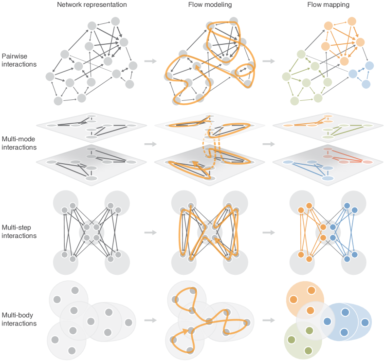
Figure 1: Modeling and mapping flow with the map equation framework. Given a complex system, the researcher first needs to choose an appropriate network representation (left column), such as a weighted and directed network to capture pairwise interactions, a multilayer network to capture multi-mode interactions, a memory network with state nodes to capture multi-step interactions, or a hypergraph to capture multi-body interactions. Then, one chooses a random walk model as a proxy for real-world flow (middle column). Finally, minimizing the map equation captures flow modules that trap a random walker for a long time before exiting (right column). Because real-world flow is intimately related to the system function, flow modules reveal the systems’ functional components.

II.1 Network representation

Complex systems comprise numerous diverse components that interact in intricate ways, making it impossible to comprehend the system’s functioning through mere observation. Network representations seek to schematize the increasingly accessible relational data by abstracting away all but the essential: nodes and links in their most basic form. The effectiveness of a network representation relies on its ability to explain the complex system through subsequent analysis, including flow-based community detection.

The map equation framework can use a variety of network representations to reliably identify flow-based communities in complex systems (Fig. 1). In the simplest case, we construct a network with binary links that indicate whether two elements interact. With more information about interactions, we can consider richer network representations: Directed and weighted networks to characterize the orientation and strength of interactions. Multilayer or multiplex networks when the problem requires distinguishing different interaction types or interactions that change over time. For capturing multi-body interactions, hypergraphs offer a suitable representation.

The research question guides how to best model the characteristics of a real-world complex system. Can a binary network capture the observed data sufficiently well, or is a weighted directed network required? Because adding weights and directions improves the model accuracy at a minimal computational cost in the map equation framework, when available we incorporate them with few exceptions. Will capturing salient temporal features require a multi-step or multi-mode representation? Are multi-body interactions indispensable for explaining system dynamics? These types of questions often require testing various network representations, comparing how they influence the flow model and the communities.

Because any network representation schematizes the raw interaction data, selecting the most suitable network representation involves a delicate balance between simplicity and accuracy: More intricate network representations prioritize accuracy at the cost of sacrificing conceptual simplicity and computational efficiency.

II.2 Flow modeling

Unless the network flows are explicit, we build a flow model on top of the network representation (Fig. 1). Modeling network flows as Markovian diffusion processes with random walks uses all the information in the network representation with minimal assumptions and can efficiently reveal flow-based communities. Higher-order generalizations of Markov processes enable incorporating the effects of multi-mode, multi-step, or multi-body interactions.

We first consider pairwise interactions and memoryless diffusion dynamics of a random walk on a network $G=\left(V,E\right)$ with nodes $V$, edges $E$, and $N=\left|V\right|$. In this setting, the network constrains the random walker’s trajectory. The transition probability $p_{uv}$ that a random walker at node $u$ visits node $v$ in the next step is proportional to the link weight $w_{uv}$ between $u$ and $v$,

$$p_{uv}=\frac{w_{uv}}{\sum_{v}w_{uv}},$$ (1)

and the stationary node visit rates are given by the recursive system of equations

$$p_{v}=\sum_{u}p_{u}p_{uv}.$$ (2)

In undirected networks, the stationary distribution of node visit rates is proportional to node strength $s$,

$$p_{v}=\frac{s_{v}}{\sum_{u}s_{u}},$$ (3)

where $s_{v}=\sum_{u}w_{uv}=\sum_{u}w_{vu}$ is node $v$’s strength. That is, the probability that the random walker visits a node is high if the node has high strength.

However, directed networks can have dangling nodes with no outgoing links or unreachable regions with no incoming links, so the node visit rates depend on where the random walker starts. In directed networks, random walks are ergodic so that Eq. 2 converges to a unique solution only if the network is strongly connected and the random walk is aperiodic. Empirical networks often do not have these properties. To overcome this issue and ensure a stationary solution in directed networks, we use teleportation and allow the random walker to teleport to a random node independent of the current node at a low rate $\tau$. Now, stationary node visit rates can be obtained by solving equations

$$p_{v}^{*}=(1-\tau)\sum_{u}p_{u}^{*}p_{uv}+\tau\varepsilon_{v}$$ (4)

with the power iteration method [19]. In Eq. 4, the parameter $\varepsilon_{v}$ represents the probability that the random walker teleports to the node $v$. This probability is uniform in the standard teleportation scheme, that is, $\varepsilon_{v}=\frac{1}{N}$ for all $v$ [20].

The drawback of this teleportation strategy is that the stationary solution $p_{v}^{*}$ depends on the choice of $\tau$. We can apply unrecorded link teleportation, so-called smart teleportation [21] for more robust results. Instead of assuming a constant probability $\varepsilon_{v}$ where a random walker teleports to any node irrespective of the network topology, link teleportation selects a link as a teleportation target at random and proportional to its weight. This leads to a teleportation parameter $\varepsilon_{v}$ proportional to a node’s incoming strength

$$\varepsilon_{v}=\frac{s_{v}^{\text{in}}}{\sum_{u}s_{u}^{\text{in}}},$$ (5)

where $s_{v}^{\text{in}}=\sum_{u}w_{uv}$ denotes the in-strength of node $v$. Link teleportation reduces the dependence on the parameter $\tau$, however, encoding teleportation steps would affect the detected community structure as this corresponds to introducing artificial links between source and target nodes. Therefore, we do not record teleportation and only record steps along existing links. This amounts to performing an extra step without teleportation on a stationary solution for recorded teleportation

$$p_{v}^{\text{unrec}}=\sum_{u}p_{u}^{*}p_{uv}.$$ (6)

For any given network representation, all these flow models are unbiased such that a random walker follows links proportional to their weights. Unbiased random walks are default flow models in the map equation framework. Some applications may benefit from a more complex flow model. For example, a biased flow model where the random walker is guided by node attributes, preferring to visit nodes with similar attributes, can more accurately model real flow statistics with desirable effects on the flow mapping.

II.3 Flow mapping

In networks with a modular structure where nodes are more strongly connected inside communities than between communities, as in the top row of Fig. 1, the random walker remains inside a community for a considerable time before exiting.

To capture these patterns, we capitalize on the correspondence between detecting regularities in data and compressing the data, formalized by the minimum description length principle. Grounded in information theory, the minimum description length principle posits that the best explanation for a data sequence is the one that provides the shortest description of that data [22]. Applying the minimum description length principle involves finding the model that can explain the data with the shortest possible code, trading off between model complexity and model fit.

To identify flow modules in the network, we aim to compress a modular description of a random walk on the network. A schematic network with four modules illustrates (Fig. 2): Placing all nodes in a single module minimizes the model complexity with a costly description of the random walker’s position among all nodes in the network. The model maximally underfits the data. A two-module solution increases the model complexity, requiring specifying movements also between modules. But communicating the random walker’s position given the module information is cheaper with fewer nodes to discern. The shortest possible description length decreases with three and four modules because the cost for model complexity increases slower than the description of the random walker’s position given the module information.

Increasing the module complexity beyond four modules leads to overfitting and higher description length. The shortest cost for specifying the position in smaller modules cannot compensate for more complex models. The model with one module for each node has the highest model complexity, maximally overfitting the data.

\begin{overpic}[width=411.93767pt]{figures/complexity-v5.pdf} \put(-2.0,18.0){\rotatebox{90.0}{{Codelength}}} \put(43.0,-2.0){{Model complexity}} \end{overpic}

Figure 2: Schematic solution landscape of varying model complexity. The leftmost one-level solution has the lowest model complexity. The rightmost singleton solution has the highest model complexity. Colors indicate module assignments, and the numbers below solutions approximate the codelengths. The solution with the lowest codelength balances model complexity and modular regularities.

III The Map Equation

To employ the minimum description length principle, we conceptually encode the random walker’s trajectory with codewords assigned to nodes. The code’s average per-step description length – we call it codelength for short – measures how well the code exploits regularities in the walker’s trajectory. In practice, however, we only consider the modular compression, that is, the codelength, but not the code itself.

Grouping nodes into modules enables reusing codewords across modules with one designated codebook per module for a shorter overall codelength. However, this requires introducing an index-level codebook as well as module-specific module-exit codewords for describing transitions between modules, increasing the overall codelength. Finding modules that describe the random walk’s regularities well and minimize the codelength means balancing between choosing small modules for efficiently describing intra-module steps and choosing modules such that there are only few links between modules for minimizing the rate at which the random walker takes inter-module steps.

Per Shannon’s source coding theorem [23], the codelength’s lower limit when not partitioning nodes into modules is the entropy over the nodes’ stationary visit rates. Applied to a network’s modular structure, the codelenght’s lower limit is the sum of the module and index-level codebooks’ entropies, weighted by the rate at which they are used.

III.1 The two-level map equation 

For a partition $\mathsf{M}$ of the nodes $u\in V$ into modules $\mathsf{m}\in\mathsf{M}$, we construct $\left|\mathsf{M}\right|$ module codebooks. Each node $u$ has a module-dependent codeword, meaning that the same codeword can be reused for nodes in other modules. For a uniquely decodable code, an additional index codebook encodes transitions into modules. The index codewords derive from the frequencies of module entries. The probability $q_{\mathsf{m}\curvearrowleft}$ that a random walker enters module $\mathsf{m}$ is

$$q_{\mathsf{m}\curvearrowleft}=\sum_{u\notin\mathsf{m},v\in\mathsf{m}}p_{u}p_{uv}.$$ (7)

Besides codewords for communicating which node a random walker visits, each module codebook requires a designated exit codeword for communicating when a random walker leaves the module. The probability $q_{\mathsf{m}\curvearrowright}$ of leaving module $\mathsf{m}$ is

$$q_{\mathsf{m}\curvearrowright}=\sum_{u\in\mathsf{m},v\notin\mathsf{m}}p_{u}p_{uv}.$$ (8)

To define the map equation, we apply Shannon’s source coding theorem to the index codebook and each module codebook. The codelength for describing movements within module $\mathsf{m}$ is

$$H(P_{\mathsf{m}})=-\frac{q_{\mathsf{m}\curvearrowright}}{p_{\mathsf{m}}^{\circlearrowright}}\log_{2}\frac{q_{\mathsf{m}\curvearrowright}}{p_{\mathsf{m}}^{\circlearrowright}}-\sum_{u\in\mathsf{m}}\frac{p_{u}}{p_{\mathsf{m}}^{\circlearrowright}}\log_{2}\frac{p_{u}}{p_{\mathsf{m}}^{\circlearrowright}},$$ (9)

where $p_{\mathsf{m}}^{\circlearrowright}=q_{\mathsf{m}\curvearrowright}+\sum_{u\in\mathsf{m}}p_{u}$ is the total use rate of module $\mathsf{m}$’s codebook. Similarly, for the index codebook, the codelength for describing random walker transitions between modules is

$$H(Q)=-\sum_{\mathsf{m}\in\mathsf{M}}\frac{q_{\mathsf{m}\curvearrowleft}}{q_{\curvearrowleft}}\log_{2}\frac{q_{\mathsf{m}\curvearrowleft}}{q_{\curvearrowleft}},$$ (10)

where $q_{\curvearrowleft}=\sum_{\mathsf{m}\in\mathsf{M}}q_{\mathsf{m}\curvearrowleft}$.

The sum of codelengths for all codebooks weighted by their use rate gives the map equation

$$L\left(\mathsf{M}\right)=q_{\curvearrowleft}H(Q)+\sum_{\mathsf{m}\in\mathsf{M}}p_{\mathsf{m}}^{\circlearrowright}H(P_{\mathsf{m}}).$$ (11)

With an increasing number of modules, the codelength of the module codebooks decreases while the codelength of the index codebook increases. The network partition that best captures the modular network flows maximally compresses the description length defined by the map equation – minimizing the map equation over all possible partitions gives the optimal partition.

III.2 The multilevel map equation

Complex systems often have a hierarchical – multilevel – organization consisting of nested modules at different levels (Fig. 3). We generalize the map equation to describe multilevel structures by applying it to each module $\mathsf{m}\in\mathsf{M}$ recursively [24, 18],

$$L(\mathsf{M})=q_{\curvearrowleft}H(Q)+\sum_{\mathsf{m}\in\mathsf{M}}L(\mathsf{m}).$$ (12)

\begin{overpic}[width=303.53267pt]{figures/nine-triangles-desaturated.pdf} \put(48.7,76.0){{\small{\color[rgb]{0.62109375,0.8046875,0.56640625}1}}} \put(35.0,52.8){{\small{\color[rgb]{0.37109375,0.671875,0.56640625}2}}} \put(62.1,52.8){{\small{\color[rgb]{0.12109375,0.51171875,0.55859375}3}}} \put(21.8,29.0){{\small{\color[rgb]{0.94140625,0.66796875,0.48046875}1}}} \put(8.7,5.0){{\small{\color[rgb]{0.9140625,0.48046875,0.3828125}2}}} \put(35.0,5.0){{\small{\color[rgb]{0.84765625,0.3046875,0.375}3}}} \put(75.4,29.0){{\small{\color[rgb]{0.6484375,0.80859375,0.8359375}1}}} \put(62.1,5.0){{\small{\color[rgb]{0.44140625,0.6171875,0.73046875}2}}} \put(88.5,5.0){{\small{\color[rgb]{0.30859375,0.37890625,0.5625}3}}} \put(48.7,60.0){{\color[rgb]{0.37109375,0.671875,0.56640625}I}} \put(21.0,14.0){{\color[rgb]{0.9140625,0.48046875,0.3828125}II}} \put(74.0,14.0){{\color[rgb]{0.44140625,0.6171875,0.73046875}III}} \end{overpic}

Figure 3: Schematic triangle network with a multilevel partition. Each small triangle (1, 2, 3) is a sub-module, organized in groups of three triangles in each top-level super-module (I, II, III).

Each module $\mathsf{m}$ contains either (i) a set of submodules or (ii) a set of nodes:

1. For a module $\mathsf{m}$ with submodules $\mathsf{m}^{\prime}\in\mathsf{m}$, the contribution to the overall codelength is

   $$L\left(\mathsf{m}\right)=q_{\mathsf{m}}^{\circlearrowright}H\left(Q_{\mathsf{m}}\right)+\sum_{\mathsf{m}^{\prime}\in\mathsf{m}}L\left(\mathsf{m}^{\prime}\right),$$ (13)

   that is, we treat each module $\mathsf{m}$ with submodules the same way as the top-level module $\mathsf{M}$, with one addition: we need to consider module exits from $\mathsf{m}$, thus defining its codebook usage rate

   $$q_{\mathsf{m}}^{\circlearrowright}=q_{\mathsf{m}\curvearrowright}+\sum_{\mathsf{m}^{\prime}\in\mathsf{m}}q_{\mathsf{m}^{\prime}\curvearrowleft}$$ (14)

   and

   $$\begin{split}H\left(Q_{\mathsf{m}}\right)=&-\frac{q_{\mathsf{m}\curvearrowright}}{q_{\mathsf{m}}^{\circlearrowright}}\log_{2}\frac{q_{\mathsf{m}\curvearrowright}}{q_{\mathsf{m}}^{\circlearrowright}}\\ &-\sum_{\mathsf{m}^{\prime}\in\mathsf{m}}\frac{q_{\mathsf{m}^{\prime}\curvearrowleft}}{q_{\mathsf{m}}^{\circlearrowright}}\log_{2}\frac{q_{\mathsf{m}^{\prime}\curvearrowleft}}{q_{\mathsf{m}}^{\circlearrowright}}.\end{split}$$ (15)

2. The codelength contribution of a module $\mathsf{m}$ that contains nodes but no further submodules is

   $$L\left(\mathsf{m}\right)=p_{\mathsf{m}}^{\circlearrowright}H\left(P_{\mathsf{m}}\right),$$ (16)

   where

   $$p_{\mathsf{m}}^{\circlearrowright}=q_{\mathsf{m}\curvearrowright}+\sum_{u\in\mathsf{m}}p_{u}$$ (17)

   and

   $$\begin{split}H(P_{\mathsf{m}})=&-\frac{q_{\mathsf{m}\curvearrowright}}{p_{\mathsf{m}}^{\circlearrowright}}\log_{2}\frac{q_{\mathsf{m}\curvearrowright}}{p_{\mathsf{m}}^{\circlearrowright}}\\ &-\sum_{u\in\mathsf{m}}\frac{p_{u}}{p_{\mathsf{m}}^{\circlearrowright}}\log_{2}\frac{p_{u}}{p_{\mathsf{m}}^{\circlearrowright}}.\end{split}$$ (18)

III.3 Challenges and remedies

\begin{overpic}[width=195.12767pt]{figures/field-of-view-limit-4.pdf} \put(0.0,95.0){a} \end{overpic}

\begin{overpic}[width=195.12767pt]{figures/ER-4.pdf} \put(0.0,95.0){b} \end{overpic}

Figure 4: Field-of-view limitations. Over-partitioning can occur in networks with (a) constrained structure, or (b) random structure. Node colors show module assignments.

Resolution limit.

Finding modules in large networks can be affected by a resolution limit that prevents detecting small modules when large modules are present. Small but functionally meaningful modules may be merged into larger ones.

For the map equation, there is an analytical estimate that relates the number of links between modules to the map equation’s resolution limit,

$$\frac{4^{l_{\mathsf{m}}}}{l_{\mathsf{m}}+1}\lesssim C$$ (19)

where $l_{\mathsf{m}}$ is the number of internal links in module $\mathsf{m}$, and $C$ is the cut size, that is, the number of links between modules [25]. However, compared to other widely-used community-detection methods, such as Modularity, where the resolution limit depends on the total number of links in the network [26], or the stochastic block model, where it depends on the total number of nodes [27], the map equation is less affected by resolution limit.

Field-of-view limitations.

Dual to the resolution limit, which can prevent detecting modules below an effective size, methods can have an upper limit in the effective size they can detect, a so-called field-of-view limit. While the map equation is less susceptible to the resolution limit than other community detection methods, the field-of-view limit can affect its performance in some networks.

The map equation’s flow-based approach implicitly assumes that modules are assortative structures where nodes with similar functions are densely connected. However, this assumption may not be valid in networks with constrained structures. For example, geographically embedded networks such as power grids or transportation networks typically contain sparse regions. The map equation tends to over-partition these regions into smaller communities [13, 28]. We illustrate a realization of this problem in Fig. 4a.

Over-partitioning can also occur in random networks created without an explicit modular structure. The map equation aims to describe the network’s structure concisely but without assuming any generative process. Consequently, the map equation identifies modular structure in random networks whose density is below a certain threshold, simply because such networks contain subgroups of nodes with low external link density [8] (Fig. 4b).

Markov time scaling.

By integrating Markov time scaling with the map equation to adjust its resolution, we can overcome the field-of-view limitations [29]. The standard map equation encodes the random walker’s position in the network after every transition; thus, the default Markov time is $t=1$. However, we can generalize the map equation to Markov times other than one by scaling the transition rates in Eq. 1 with the Markov time $t$

$$p_{uv}\left(t\right)=tp_{uv},$$ (20)

and if $t<1$, we additionally account for

$$p_{uu}\left(t\right)=\left(1-t\right)+tp_{uu}.$$ (21)

The Markov time controls how many steps a random walker can take before we encode its position. For $t<1$, the random walker visits the same node several times because it moves slower, resulting in smaller modules. For $t>1$, the walker moves faster and can take more than one step before encoding its position such that not every node along the trajectory is encoded, favoring larger modules.

Variable Markov time scaling.

Variable Markov time [30] relaxes the constraints of a global Markov time parameter: choosing between detecting large-scale structures above the field-of-view limit or highlighting small dense structures. The basic idea is to adjust the Markov time dynamically based on the random walker’s current neighborhood in the network, allowing it to move faster in sparse areas and slower in dense areas, reducing the effects of both the field-of-view limit and the resolution limit simultaneously. Adjusting the random walker’s Markov time dynamically enables capturing a broader range of modular flow patterns within a single map.

To scale the Markov time dynamically, we adjust the flow between nodes with a node-local Markov time $t_{u}$ that is inversely proportional to the flow of node $u$. As a baseline, we use the densest part of the network and keep the minimum Markov time at 1 to avoid the resolution limit. We define the variable Markov time $t_{u}$ for node $u$ as the ratio between the maximum flow over all nodes, $p_{\text{max}}$, and the local flow $p_{u}$,

$$t_{u}=\frac{p_{\text{max}}\,k_{\text{tot}}}{\min(1,p_{u}k_{\text{tot}})},$$ (22)

where $k_{\text{tot}}=\sum_{u}k_{u}$ is the total node degree over all nodes in the network. However, in real-world networks where most nodes typically have few links and a few nodes have many links, this definition of variable Markov time is sensitive to the degree of the strongest node. We can address this issue by taking the logarithm with base 2 of $p_{\text{max}}$ and $p_{u}$ instead to avoid small Markov times, resulting in a variable Markov time where the random walker moves with a constant entropy rate,

$$t_{u}=\frac{\log_{2}\left(p_{\text{max}}\,k_{\text{tot}}\right)}{\min\left(1,\log_{2}\left(p_{u}\,k_{\text{tot}}\right)\right)}.$$ (23)

For directed links, we scale the flow with the Markov time of the source nodes. To keep the minimum Markov time at $1$ for undirected links, we scale the flow with the minimum Markov time $t_{uv}=\min(t_{u},t_{v})$ between nodes $u$ and $v$. Typically, networks with less skewed degree distribution can benefit from using Eq. 22 to avoid the field-of-view limit.

\begin{overpic}[width=433.62pt]{figures/algorithm-v2.pdf} \put(21.0,96.0){a} \put(41.0,96.0){b} \put(61.0,96.0){c} \put(21.0,73.0){d} \put(41.0,73.0){e} \put(61.0,73.0){f} \put(0.5,47.0){g} \put(21.0,47.0){h} \put(41.0,47.0){i} \put(61.0,47.0){j} \put(0.5,21.2){k} \put(21.0,21.2){l} \put(41.0,21.2){m} \put(61.0,21.2){n} \end{overpic}

Figure 5: Schematic search algorithm for two-level partitions. Infomap utilizes a greedy stochastic search algorithm to optimize the map equation by minimizing codelength, allowing the discovery of modular regularities. The algorithm comprises multiple strategies to avoid local minima, starting with node assignments to modules (a) and iteratively moving nodes to neighboring or new modules if it reduces the codelength (b–f). Furthermore, the algorithm incorporates fine-tuning (g–j) and coarse-tuning (k–n) steps to improve module assignments at various levels of granularity.

IV Infomap

Infomap is a greedy stochastic search algorithm designed to minimize the map equation and detect two-level and multilevel flow communities in networks [24, 17]. Since community detection is an NP-hard combinatorial optimization problem, Infomap cannot guarantee to find the map equation’s global minimum; it uses iterative and recursive optimization heuristics to avoid local minima and is known to achieve good results in practice [8, 9, 10]. The Infomap search algorithm is inspired by the Louvain algorithm for modularity maximization [31] but uses additional fine-tuning and coarse-tuning steps, similar to how the Leiden algorithm later refined Louvain [32]. When expressed in differentiable tensor form with soft cluster assignments, the map equation can also be optimized with graph neural networks [33]. Infomap is available as an open-source software package [16].

Infomap runs in two phases: the first phase creates a two-level partition, and the second phase creates a multilevel partition. Depending on the use case, Infomap can stop either after the two-level phase and output a two-level partition or after the multilevel phase for a multilevel partition if it improves the two-level solution.

IV.1 The two-level phase 

The two-level phase consists of two stages:

In stage 1, first, Infomap assigns each node to its own module, creating a trivial partition with high codelength as a starting point (Fig. 5a). Such a partition of singletons places all links between modules – assuming the network has no self-loops – and forces the random walker to switch modules with every step, inefficiently compressing the random walker’s trajectory. Second, Infomap updates the partition iteratively and considers moving nodes in random order to either of their neighboring modules or a new singleton module (Fig. 5b). To avoid re-checking nodes with stable module assignments, Infomap initially marks all nodes as candidates for moving. Then, as long as there are candidates left, Infomap randomly chooses a candidate and tries to move it to reduce the codelength by some adjustable minimum amount. If there are several possible moves for a node, Infomap chooses the one that reduces the codelength the most. When Infomap moves a node, it marks that node and all its neighbors as candidates for moving. A node that has no improving move is unmarked. When no candidate nodes are left, Infomap stops moving individual nodes (Fig. 5c). Third, Infomap repeats the second step, now moving the identified modules: nodes that belong to the same module are moved into or out of other modules together as a group. This step repeats with larger and larger modules as long as the codelength decreases (Fig. 5d–f). We call stage 1 Infomap’s core algorithm.

In stage 2, Infomap tunes the partition to avoid local minima by alternating between fine-tuning and coarse-tuning steps. Fine-tuning and coarse-tuning follow the same principle and use the core algorithm, but they consider different objects to move. For fine-tuning, Infomap uses the core algorithm to move individual nodes to improve the codelength (Fig. 5g–j). For coarse-tuning, Infomap partitions all modules individually into sub-modules using the core algorithm and then moves these sub-modules to reduce the codelength (Fig. 5k–n). Infomap fine- and coarse-tunes at least once and stops when it cannot improve the codelength by some minimum amount: either by an absolute value or a relative value determined from the codelength of the one-level partition, both of which can be adjusted.

IV.2 The multilevel phase

The multilevel phase aims to reduce the codelength by adding further index levels to a two-level partition. It contains two stages.

In stage 1, Infomap compresses inter-module transitions by first aggregating the network at the module level. This creates a network where nodes represent the previous modules, and inter-module links are merged. Second, Infomap uses the two-level algorithm to partition the aggregated network. The resulting two-level partition comprises a three-level partition when interpreted in the context of the network before aggregation. Infomap repeats stage 1 as long as aggregating and partitioning the network and adding one more index level per iteration yields a non-trivial solution.

In stage 2, Infomap partitions the modules at the highest level of the multi-level partition recursively. Since the lower levels in the partition were designed from a perspective that did not consider the higher levels, they may be suboptimal and suffer from resolution issues. Moreover, the resulting partition is balanced, and all modules have the same depth, which is generally not the case in real-world networks. To overcome this, Infomap keeps the modules at the highest level but forgets their submodules to re-partition each module independently, using the full algorithm, that is, the two-level phase followed by the multi-level phase.

\begin{overpic}[width=433.62pt]{figures/solution_landscape_jazz_d=0.02_a=0.9.pdf} \put(77.0,28.0){\footnotesize{Cluster size}} \put(60.0,6.0){\footnotesize{{Cluster id (cluster size)}}} \put(60.0,2.0){\footnotesize{Codelength (bits)}} \end{overpic}

Figure 6: The solution landscape of the jazz network. Visualization of clusters of partitions and the codelength of the best partition in each cluster. Cluster 1 has two partitions and the shortest codelength. Clusters 2–4 have a slightly higher codelength and comprise 17 partitions. Differences between partitions of similar quality can reveal important aspects of the underlying data.

IV.3 Solution landscape 

Even though Infomap is designed to avoid converging to a local minimum, the non-convex properties of the map equation can be a problem in practice. Moreover, local minima can have a codelength close to the global minimum, which can be an inherent property of the studied system, or be caused by noisy data or sensitivity to model parameters.

To study the map equation’s solution landscape, we visualize the detected minima [34]. We run Infomap repeatedly and with different seeds to generate different partitions which we cluster to identify the partition clusters in the map equation’s solution landscape. We consider the solution landscape complete when new partitions fall within already identified partition clusters with a high probability. Reaching a complete landscape also answers how many times we need to run Infomap to find all relevant solutions. To measure distances between partitions, we use a Jaccard-based metric that allows using two-level or multilevel partitions. By varying the cluster distance threshold we can explore the solution landscape at different scales.

Figure 6 shows a two-dimensional embedding of the jazz network’s [35] solution landscape, created with UMAP [36]. The jazz network’s solution landscape has several local minima with codelengths close to the global minimum. If these alternative partitions differ in any aspect important to the researcher – compared to each other or the global minimum – they can reveal important aspects of the underlying data. In contrast, the solution landscape of the Zachary karate club network [37] has only one partition, that is, Infomap always converges to the same solution.

V The map equation for higher-order networks

Higher-order network models can provide a more accurate representation of complex systems by capturing dynamics beyond pairwise interactions [38, 39]. These networks have found applications in various fields where conventional network models may fall short. For example, conventional networks may struggle to represent protein–protein interactions, where three or more proteins can form complexes. Similarly, they may not adequately capture the dynamics of social networks, where the information flow depends on its source.

To address these limitations, the higher-order map equation framework introduces so-called state nodes to represent higher-order dependencies and generalizes Markovian dynamics from first to higher order. State nodes can reflect various aspects of the system, such as different layers in multilayer networks or previously visited physical nodes in memory networks. Physical nodes correspond to regular nodes in first-order networks and represent the interacting entities.

We use the map equation to partition nodes into communities that minimize the description of random walker movements between state nodes. This generalization does not impact the index codebook but necessitates modifications to the module codebooks. When multiple state nodes of the same physical node are assigned to the same module, they share the same codeword to ensure they represent the same object. At the same time, state nodes of the same physical node assigned to different modules allow identifying overlapping modules.

We discuss various higher-order models focusing on memory networks, multilayer networks, temporal networks, and hypergraphs. While the map equation directly supports multilayer and memory networks, temporal networks and hypergraphs require additional modeling choices. We build on the memory and multilayer map equation and incorporate additional constraints into the random-walk model to capture the intricacies of temporal and multi-body interactions.

V.1 Memory networks 

\begin{overpic}[width=130.08731pt]{figures/memory-a-2.pdf} \put(0.0,108.0){a} \end{overpic}

\begin{overpic}[width=130.08731pt]{figures/memory-b-2.pdf} \put(0.0,108.0){b} \end{overpic}

\begin{overpic}[width=130.08731pt]{figures/memory-c-2.pdf} \put(0.0,108.0){c} \end{overpic}

Figure 7: Two-step paths represented as a memory network. Two-step paths (a) are realized as a first-order network in (b) and a second-order memory network using state nodes in (c). Each state node represents the memory of the previous step: The path $\mathsf{A-C-D}$ is represented by the state node $\mathsf{A}$ in physical node $\mathsf{C}$ connected to the state node $\mathsf{C}$ in $\mathsf{D}$. With more pathway data, each physical node may comprise multiple state nodes. The memory network can be partitioned into overlapping modules by assigning the state nodes belonging to the same physical node to different modules.

In a $k$-th order memory network, the random walker’s next step depends on the $k-1$ previously visited nodes

$$P_{uv}=P(v|u,u_{-1},\dots,u_{-k+1}),$$ (24)

where $u$ is the current node, $u_{-1}$ the previous node, and $u_{-k}$ the node visited $k$ steps ago. Modeling with memory networks enables representing flow phenomena such as high return probabilities. Memory networks have been used successfully in various domains, including modeling citation pathways through multidisciplinary journals and traffic flow through transit airports [40, 41].

We illustrate the approach using flows from two domains through a central node $\mathsf{C}$ (Fig. 7a). Conventional first-order networks cannot model the flow dependency on its origin, resulting in undesired mixing (Fig. 7b). In contrast, a second-order memory network overcomes this limitation and encodes the history of previously visited physical nodes in state nodes: Here, the state node $\mathsf{A}$ in physical node $\mathsf{C}$ represents the transition from $\mathsf{A}$ to $\mathsf{C}$ (Fig. 7c). Using state nodes allows us to separate between flows that mix in physical node $\mathsf{C}$ and identify two overlapping modules.

\begin{overpic}[width=433.62pt]{figures/multilayer-models-alt.pdf} \put(0.0,20.0){a} \put(34.0,20.0){b} \put(68.0,20.0){c} \put(98.7,12.0){$r$} \end{overpic}

Figure 8: Multilayer network models with (a) explicit multilayer links, (b) intra- and inter-layer links, and (c) intra-layer links and inter-layer relax rate.

Memory networks from first-order data.

To obtain a stationary flow distribution for state nodes in a memory network, we require sequence data; ideally, empirical multi-step data. However, in cases where such data are unavailable, we can model higher-order data on top of first-order networks to reveal overlapping modules. This approach offers a valuable alternative for identifying patterns in complex systems with higher-order dependencies, even in the absence of empirical multi-step data.

For example, we can use the second-order random walk model known as node2vec [42] to create state nodes. In this model, the return parameter $p$ controls the probability of flows returning to where they came from, while the in-out parameter $q$ controls the probability of flows staying in the vicinity or moving further away from where they came from. By tuning $p$ and $q$, flows can be directed to stay more local to where they came from, reinforcing triangles [43]. To avoid the curse of dimensionality when representing every possible second-order pathway as state nodes, a sparse, variable-order memory network can be employed where the number of state nodes for each physical node is determined using an information-loss criterion [43].

V.2 Multilayer networks 

Real-world systems are often characterized by flows that can be stratified across different layers. For example, individuals may use different modes of transport to commute between cities or communicate with each other using various messaging or social media platforms. To model such multilayer flows, we utilize multilayer networks where each physical node can exist in many layers with different link structures. A group of nodes with similar connectivity patterns across different layers should be assigned to the same community. However, if the connectivity patterns of a physical node vary across the layers, it should be assigned to multiple communities.

The map equation interprets a multilayer network with $l$ layers as an $l$-th-order memory network where state nodes assigned to a physical node correspond to different layers [44]. When connecting multilayer state nodes, we distinguish two types of links: intra-layer links, which connect nodes within the same layer, and inter-layer links, which connect nodes across different layers. Depending on the input data, there are three ways to define inter-layer links.

Explicit multilayer links.

If the data provide explicit information about the link weight $w_{u^{A}v^{B}}$ between node $u$ in layer $A$ and node $v$ in layer $B$ (Fig. 8a), we can directly obtain a stationary flow distribution for the state nodes. The transition probability between any two state nodes $u^{A}$ and $v^{B}$ is

$$p_{u^{A}v^{B}}=\frac{w_{u^{A}v^{B}}}{\sum_{v^{B}}w_{u^{A}v^{B}}}.$$ (25)

Intra- and inter-layer links.

In some cases, the data does not provide explicit multilayer links between all pairs of state nodes. Instead, it may provide explicit links within layers, and inter-layer link weights $\upsilon_{u^{A}u^{B}}$, which describe the coupling between physical node $u$ in layers $A$ and $B$ when $A\neq B$ (Fig. 8b). In this model, the random walker moves between layers proportional to inter-layer link weight, but we do not encode this movement. The map equation expands the inter-layer links to multilayer links, and the transition probability is

$$p_{u^{A}v^{B}}=\frac{\upsilon_{u^{A}u^{B}}}{\sum_{B}\upsilon_{u^{A}u^{B}}}\frac{w_{u^{B}v^{B}}}{\sum_{v}w_{u^{B}v^{B}}},$$ (26)

where $\upsilon_{u^{A}u^{A}}=\sum_{v}w_{u^{A}v^{A}}$.

Intra-layer links and inter-layer relax-rate.

In most cases, empirical inter-layer links are not provided. To relax the layer constraints and allow the random walker to move without inter-layer links, the map equation introduces a relax rate parameter $r$ (Fig. 8c). In this model, the random walker follows intra-layer links with a probability $1-r$ and moves between layers with a probability $r$. The transition probabilities become

$$p_{u^{A}v^{B}}=\left(1-r\right)\delta_{AB}\frac{w_{u^{A}v^{B}}}{\sum_{v^{B}}w_{u^{A}v^{B}}}+r\frac{w_{u^{A}v^{B}}}{\sum_{A}\sum_{v^{B}}w_{u^{A}v^{B}}},$$ (27)

where $\delta$ is the Kronecker delta.

V.3 Modeling temporal data 

\begin{overpic}[width=433.62pt]{figures/temporal-network.pdf} \put(0.0,52.0){a} \put(35.0,52.0){b} \put(69.0,52.0){c} \end{overpic}

Figure 9: Standard network models destroy temporal information. (a) Drawing interactions along a time axis shows that the orange random walker moves back in time, thus breaking causality. The blue random walker guided by state nodes obeys causality. (b) Conventional first-order network models allow the orange random-walker step because they do not model temporal dependencies. (c) Memory networks constrain temporal flows according to available data.

Memory and multilayer networks offer two alternatives to capture higher-order dependencies in temporal network data. Memory networks capture causal paths that standard networks wash out [45]. For example, $\mathsf{A}$ can only causally influence $\mathsf{C}$ through $\mathsf{B}$ if $\mathsf{A}$ influences $\mathsf{B}$ before $\mathsf{B}$ influences $\mathsf{C}$, but conventional first-order networks discard temporal ordering and distort essential flow dynamics critical for unveiling system functions (Fig. 9). In contrast, state nodes in memory networks preserve temporal ordering.

When dealing with network snapshots across different time intervals rather than pathway data, we model the data with a temporal multilayer network. Such a model allows us to represent the network’s evolution over time by organizing snapshots into distinct layers and enables analyzing, for example, temporal communities in ecological systems and fossil record data [46, 47]. In these systems, inter-layer links are typically absent; instead, a relaxation rate models random-walker transitions between layers. To control temporal ordering in multilayer networks explicitly, the map equation can apply layer constraints to restrict the random walker to jump only to layers within a specific temporal distance [48].

Furthermore, an adapted version of the map equation captures intermittent communities that emerge and dissolve repeatedly and independently from other communities in the network [48]. Because the multilayer map equation couples entire layers, it cannot accurately capture flow persistence within groups of nodes whose existence is time-dependent, making it difficult to identify intermittent communities. To address this scenario, we use node-level layer coupling: Node-level layer coupling estimates the coupling strength $\upsilon_{u^{A}u^{B}}$ between node $u$ in layers $A$ and $B$ based on how similar $u$’s connectivity patterns are in these two layers, quantified using the Jensen-Shannon divergence (JSD):

$$\upsilon_{u^{A}u^{B}}=1-JSD(p_{u^{A}},p_{u^{B}}),$$ (28)

where $p_{u^{A}}=(p_{u^{A}v_{1}^{A}},\dots,p_{u^{A}v_{N}^{A}})$ represents the intra-layer probabilities that a random walker steps from node $u$ in layer $A$ to other nodes $v$ in layer $A$.

V.4 Modeling multi-body interactions 

We can identify modules in hypergraphs by representing random walks on hypergraphs as walks on conventional or multilayer networks. However, different systems and research questions necessitate different random-walk and hypergraph models. Hyperedges can have weights, and nodes can have hyperedge-dependent weights [49]. Random walks can be lazy, allowing multiple consecutive visits to the same node, or non-lazy, forcing it to move on [50]. Additionally, these random-walk models can be represented using various network types, such as bipartite, unipartite, or multilayer networks. What network representation to choose depends on the research question, as each has different advantages.

We model flows on hypergraphs with random walks, using hypergraphs with nodes $V$, hyperedges $E$ with weights $\omega$, and hyperedge-dependent node weights $\gamma$. Each hyperedge $e$ has a weight $\omega(e)$. Each node $u$ has a weight $\gamma_{e}(u)$ for each hyperedge $e$ incident to $u$.We denote node $u$’s total incident hyperedge weight $d(u)=\sum_{e\in E(u)}\omega(e)$ and hyperedge $e$’s total node weight $\delta(e)=\sum_{u\in e}\gamma_{e}(u)$. With these weights, a lazy random walker moves from node $u$ to $v$ in three stages (Fig. 10)[49],

1. Picking hyperedge $e$ among node $u$’s hyperedges $E(u)$ with probability $\frac{\omega(e)}{d(u)}$.

2. Picking one of the hyperedge $e$’s nodes $v$ with probability $\frac{\gamma_{e}(v)}{\delta(e)}$.

3. Moving to node $v$.

Variations include non-lazy walks, which never visit the same node twice in a row, with a modified second stage

1. Picking one of hyperedge $e$’s nodes $v\neq u$ with probability $\frac{\gamma_{e}(v)}{\delta(e)-\gamma_{e}(u)}$,

\begin{overpic}[width=433.62pt]{figures/mappinghypergraphs-alt.pdf} \put(0.0,78.0){a} \put(45.0,78.0){b} \put(0.0,38.0){c} \put(45.0,38.0){d} \end{overpic}

Figure 10: Schematic hypergraph represented with three types of networks. (a) The schematic hypergraph with weighted hyperedges and hyperedge-dependent node weights. White circles labeled from $a$ to $j$ represent nodes, and large circles represent hyperedges incident to the nodes in each circle. Thin hyperedge borders for weight 1, medium for weight 2, and thick borders for weight 3. No node borders for node weight 1, thick borders for aggregated weights larger than 1. A random walk depicted with an arrow on the schematic hypergraph represented on: (b) a bipartite network where the unlabelled nodes represent the hyperedges, (c) a unipartite network, and (d) a multilayer network with grey circles defining each layer. Node colors indicate optimized module assignments and the links’ thicknesses are proportional to the random walk’s transition rates.

Bipartite.

Bipartite networks offer the most direct representation of the basic three-stage random-walk process. We represent the hyperedges with hyperedge nodes, and the three stages become a two-step walk between the nodes at the bottom and the hyperedge nodes at the top in Fig. 10b. First, a step from a node $u$ to a hyperedge node $e$,

$$P_{ue}=\frac{\omega(e)}{d(u)},$$ (29)

and then a step from the hyperedge node to a node $v$,

$$P_{ev}=\frac{\gamma_{e}(v)}{\delta(e)}.$$ (30)

For non-lazy walks, we let each incoming link to a hyperedge node connect to a state node with out-links to all of the hyperedge’s nodes except the incoming link’s source node.

Unipartite.

To represent the random walk on a unipartite network, we project the three-stage random-walk process down to a one-step process between the nodes and describe it with the transition rate matrix

$$P_{uv}=\sum_{e\in E(u,v)}P_{ue}P_{ev}=\sum_{e\in E(u,v)}\frac{\omega(e)}{d(u)}\frac{\gamma_{e}(v)}{\delta(e)},$$ (31)

where $E(u,v)$ is the set of hyperedges incident to both nodes $u$ and $v$. Each hyperedge forms a fully connected group of nodes (Fig. 10c). Unipartite networks for non-lazy walks have no self-links. The unipartite representation forms a weighted one-mode projection of the bipartite representation and requires more links with its fully connected groups of nodes.

Multilayer.

To represent the random walk on a multilayer network, we project the three-stage random-walk process down to a one-step process on state nodes in separate layers. Each hyperedge $e$ with weight $\omega(e)$ forms a layer $A$ with weight $\omega(A)$. A state node $u^{A}$ represents $u$ in each layer $A\in{E}(u)$ that contains the node. All state nodes in the same layer form a fully connected set (Fig. 10d). The transition rate between state node $u^{A}$ in layer $A$ and state node $v^{B}$ in layer $B$ is

$$P_{uv}^{AB}=\frac{\omega(B)}{d(u)}\frac{\gamma_{B}(v)}{\delta(B)}\text{ for }B\in E(u,v).$$ (32)

With one state node per hyperedge layer that contains the node, the multilayer representation requires the most nodes and links to describe the walk. Variations include walks that are biased to similar hyperedges [51].

These network representations and random-walk models have different advantages [51, 52]. The bipartite network representation enables the most efficient community detection in terms of computation time because it uses the fewest links and often results in shallower solutions. Multilayer network representations reinforce flows within similar layers, giving the deepest modular structures with the most overlap. However, this increase in detected modules comes at a high computational cost, as combining fully connected layers with other layers requires more nodes and links than the bipartite network representation. If the research question does not call for hyperedge assignments or overlapping modules, the unipartite network representation offers a trade-off with intermediate compactness, speed, and the ability to reveal modular regularities. Among random-walk models, lazy walks typically give more modules in deeper nested structures, while non-lazy walks result in higher modular overlap.

VI Networks with node attributes

Nodes in real-world networks are often labeled with additional information, such as a person’s age, an animal’s species, an object’s shape, or, more generally, as belonging to a certain category. We can characterize the dynamic process that operates on such an annotated network better by incorporating node-type information in the flow modeling or flow mapping step.

VI.1 Bipartite networks 

Bipartite networks have two different node types, left nodes $V_{L}$ and right nodes $V_{R}$, and their links only connect nodes with different types. Consequently, random walks on bipartite networks alternate between left and right nodes. While the map equation and Infomap can handle bipartite networks without including this information, it enables describing the random walk more efficiently by using pairs of codebooks for left-to-right and right-to-left transitions. To keep track of which codebook to use, we need to remember the random walker’s current node type. Using such pairs of notebooks reduces the codelength because each codebook only needs to assign codewords to half of the nodes on average. The bipartite map equation directly reflects this idea [53],

$$L_{B}\left(\mathsf{M}\right) =q_{\curvearrowleft}^{R}H\left(Q^{R}\right)+\sum_{\mathsf{m}\in\mathsf{M}}p_{\mathsf{m}}^{R\circlearrowright}H\left(P_{\mathsf{m}}^{R}\right)$$

$$+q_{\curvearrowleft}^{L}H\left(Q^{L}\right)+\sum_{\mathsf{m}\in\mathsf{M}}p_{\mathsf{m}}^{L\circlearrowright}H\left(P_{\mathsf{m}}^{L}\right).$$ (33)

Here, $Q^{R}$ and $Q^{L}$ are the left-to-right and right-to-left module entry rates, respectively; $P_{\mathsf{m}}^{R}$ and $P_{\mathsf{m}}^{L}$ are the sets of right and left node visit rates in module $\mathsf{m}$, including the left-to-right and right-to-left module exit rates, respectively; and $q_{\curvearrowleft}^{R}$ and $q_{\curvearrowleft}^{L}$ are the rates at which the left-to-right and right-to-left index level codebooks are used, respectively.

To control at which rate the bipartite node types are used, we introduce a node-type forgetting parameter $\alpha$. Assuming that we misremember node types with probability $\alpha$, the available amount of information about node types is $I=1-H\left(\alpha,1-\alpha\right)\leavevmode\nobreak\ \text{bits}$. Because of this uncertainty about node types, we interpret node visit rates as pairs of left and right flow, leading to mixed visit rates $p_{\alpha,u}=\left(\left(1-\alpha\right)p_{u},\alpha p_{u}\right)$ for left nodes $u\in V_{L}$, and $p_{\alpha,v}=\left(\alpha p_{v},\left(1-\alpha\right)p_{v}\right)$ for right nodes $v\in V_{R}$. We define the bipartite map equation with varying node-type memory for two-level partitions $\mathsf{M}$ [53],

$$L_{\alpha}\left(\mathsf{M}\right)=q_{\alpha,\curvearrowleft}H\left(Q_{\alpha}\right)+\sum_{\mathsf{m}\in\mathsf{M}}p_{\alpha,\mathsf{m}}^{\circlearrowright}H\left(P_{\alpha,\mathsf{m}}\right),$$ (34)

where $q_{\alpha,\curvearrowleft}$ is the mixed rate at which the index codebook is used, $Q_{\alpha}$ is the set of mixed module entry rates, and $p_{\alpha,\mathsf{m}}^{\circlearrowright}$ is the mixed rate at which module $\mathsf{m}$’s codebook is used. As before, we can generalize Eq. 34 to multilevel partitions through recursion.

We recover the standard map equation (Eq. 11) for $\alpha=\frac{1}{2}$, and the bipartite map equation (Eq. 33) for $\alpha\in\left\{0,1\right\}$, where setting $\alpha=1$ flips the node types. By using node-type information at rates between $I=0\leavevmode\nobreak\ \text{bits}$ and $I=1\leavevmode\nobreak\ \text{bit}$, we change the map equation’s resolution and detect communities at different scales.

VI.2 Networks with metadata 

To combine additional metadata with the network structure, we can modify the flow mapping step by extending the map equation with an additional metadata codebook [54] or the flow modeling step by choosing which random-walker steps to encode depending on the metadata [55]. Alternatively, we can use metadata as a part of an empirical prior for a Bayesian estimate of the random walker’s transition rates [56] (see SectionVII).

For simplicity, we assume unipartite networks and categorical metadata labels and denote node $u$’s label by $\ell_{u}$. Further, let $\mathcal{L}$ be the set of possible metadata labels.

The content map equation.

In addition to communicating the random walker’s current node, the content map equation requires encoding the current node’s metadata label [54]. Given a partition $\mathsf{M}$, the metadata label $\ell$ appears with frequency

$$r_{\mathsf{m},\ell}=\sum_{u\in\mathsf{m},\ell_{u}=\ell}p_{u}$$ (35)

within module $\mathsf{m}\in\mathsf{M}$. The total metadata weight of module $\mathsf{m}$ is

$$r_{\mathsf{m}}^{\circlearrowright}=\sum_{\ell\in\mathcal{L}}r_{\mathsf{m},\ell}=\sum_{u\in\mathsf{m}}p_{u}.$$ (36)

The entropy for encoding the metadata labels for the nodes along the random walker’s trajectory in module $\mathsf{m}$ is

$$H\left(R_{\mathsf{m}}\right)=-\sum_{\ell\in\mathcal{L}}\frac{r_{\mathsf{m},\ell}}{r_{\mathsf{m}}^{\circlearrowright}}\log_{2}\frac{r_{\mathsf{m},\ell}}{r_{\mathsf{m}}^{\circlearrowright}},$$ (37)

where $R_{\mathsf{m}}$ is the set of metadata frequencies in module $\mathsf{m}$. Combining Eq. 37 with Eq. 11 gives the so-called content map equation,

$$L\left(\mathsf{M}\right)=q_{\curvearrowleft}H\left(Q\right)+\sum_{\mathsf{m}\in\mathsf{M}}p_{\mathsf{m}}^{\circlearrowright}H\left(P_{\mathsf{m}}\right)+\eta\sum_{\mathsf{m}\in\mathsf{M}}r_{\mathsf{m}}^{\circlearrowright}H\left(R_{\mathsf{m}}\right),$$ (38)

where $\eta$ is a parameter to control the metadata entropy’s weight.

The content map equation encourages modules with small numbers of metadata categories since this corresponds to low metadata entropy. It typically splits structural modules into sub-modules based on their metadata labels but does not merge nodes with the same metadata label from different structural modules [55].

Metadata-dependent encoding of random walks.

\begin{overpic}[width=433.62pt]{figures/metadata-walk.pdf} \put(0.0,64.0){a} \put(38.0,64.0){b} \put(77.0,64.0){c} \end{overpic}

Figure 11: Random walks with metadata-dependent encoding probabilities. In this schematic example with a single, long random walk, we encode the random walker’s next step if the target node’s metadata are the same as for the previously encoded node. When the metadata differ, encoding with a probability between $\frac{1}{3}$ and $1$ gives the solution in (a), between $0.1$ and $\frac{1}{3}$ the solution in (b), and less than $0.1$ the solution in (c). Node shapes represent metadata, and node colors optimal partitions. The random walks are colored by the currently encoded module and labeled with circles when they encode a transition and dotted lines when they skip nodes. The alphabetic codes represent the walks with this metadata-dependent encoding scheme.

To map nonlocal relationships between metadata and network structure, we use a metadata-dependent encoding of random walks [55]. For a random walker starting at node $u$ and stepping to node $v$, we encode the step with probability $\epsilon\left(\ell_{u},\ell_{v}\right)$, which depends on the metadata labels at the start node $u$ and the currently visited node $v$, or the random walker continues without encoding to another node, say $v^{\prime}$. We encode the step to $v^{\prime}$ with probability $\epsilon\left(\ell_{u},\ell_{v^{\prime}}\right)$, or the random walker continues in the same fashion until we eventually encode the step from the start node $u$ to the currently visited node. After encoding, the random walker restarts at a random node $u^{\prime}$ chosen proportionally to the node’s visit rate.

Varying the coding this way, we derive a metadata-dependent encoding graph from a given network: The nodes are the same as in the original network, and the links derive from the coding behavior, which can connect disconnected nodes in the original network. The link weights correspond to the fractions of time that we encode each respective link, such that the weight of link $\left(u,v\right)$ is the number of times that we encode a step to $v$ after restarting at $u$, divided by the total number of encoded steps. Effectively, this yields a metadata-dependent transition matrix and metadata-dependent visit rates, which we use to detect modules with Infomap. Unlike the content map equation, modeling metadata-dependent flow enables grouping nodes that belong to different structural modules in the original network.

\begin{overpic}[width=433.62pt]{figures/illustration-regularization-5.pdf} \put(0.0,27.0){a} \put(35.5,27.0){b} \put(72.0,27.0){c} \end{overpic}

Figure 12: Community detection in an undirected weighted network with complete and missing link observations. (a) The map equation identifies two modules in a complete network with accurate network flows. (b) Missing link observations introduce inaccuracies leading to overfitting. (c) The map equation with regularized network flows recovers the complete network’s community structure. Colors represent community assignments. The width of the lighter lines represents teleportation weight, and the size of the lighter node centers indicates teleportation probability. Figure adapted from Ref. [56].

The encoding probability function determines what specific patterns the metadata-dependent encoding graph captures (Fig. 11). For example, $\epsilon\left(\ell_{u},\ell_{v}\right)=1$ forces the walker to encode every step regardless of metadata labels, equivalent to the standard map equation. Setting $\epsilon\left(\ell_{u},\ell_{v}\right)=\delta_{\ell_{u},\ell_{v}}$, where $\delta$ is the Kronecker delta, encodes only on nodes with the same metadata labels, splitting the network into modules purely based on metadata while ignoring link patterns. For binary metadata labels, a versatile choice is

$$\epsilon\left(\ell_{u},\ell_{v}\right)=p\delta_{\ell_{u},\ell_{v}}+\frac{p}{c}\left(1-\delta_{\ell_{u},\ell_{v}}\right),$$ (39)

where $p\in\left[0,1\right]$ and $c\in\left[p,\infty\right]$. Setting $c>1$ gives assortative, and setting $p<c<1$ gives disassortative modules. For $c=1$, the expression simplifies to $\epsilon\left(\ell_{u},\ell_{v}\right)=p$ without metadata dependence. The metadata-dependent encoding probability function can also take real-valued or vectorial metadata labels [55].

Metadata-dependent random walk encoding can capture nonlocal interactions, include different metadata types, and model different metadata roles. This flexibility comes at a cost, requiring generating a metadata-dependent transition graph. The content map equation is less flexible but does not require generating a transition matrix and is implemented in Infomap.

VII Networks with incomplete data 

In the previous sections, we discussed how to take advantage of the available data and identify flow models that best describe modular regularities. Once we have chosen a flow model, the standard map equation estimates stationary flow distribution based on what it sees in the data. However, data can be noisy with incomplete link measurements, leading to inaccurate estimates of the actual stationary flow distribution in the system. Consequently, when missing observations distort the balance between module and index-level codebooks, the map equation can overfit to the noise and highlight spurious communities [57, 58, 56]. We can extend the map equation to deal with incomplete data by applying a Bayesian method to regularize the random walker’s transition rates (Fig. 12) [56].

VII.1 Bayesian estimate of transition rates

We assume that a random walker steps from node $u$ to nodes $v$ proportional to $\tilde{p}_{u}=(\tilde{p}_{uv_{1}},\dots,\tilde{p}_{uv_{N}})$. The link weights $(w_{uv_{1}},\dots,w_{uv_{N}})$ represent a sample of the hidden distribution $\tilde{p}_{u}$. We assume non-negative integer weights for simplicity, but the method also works for non-negative real weights. If we interpret the transition probability $p_{uv}$ given by Eq. 1 as a maximum likelihood estimate of $\tilde{p}_{uv}$, $p_{uv}$ can deviate significantly from $\tilde{p}_{uv}$ in the case of noisy data. To reduce the effects of statistical fluctuations, we estimate the average posterior transition rates

$$\hat{p}_{uv}\left(w\right)=\int\tilde{p}_{uv}P(\tilde{p}_{u}|w_{uv_{1}},\dots,w_{uv_{N}})d\tilde{p}_{u},$$ (40)

where $P(\tilde{p}_{u}|w_{uv_{1}},\dots,w_{uv_{N}})$ is a posterior over the unknown distribution $\tilde{p}_{u}$ given by Bayes’ rule. As prior distribution $P(\tilde{p}_{u})$, we choose the Dirichlet distribution, which is the conjugate prior of the multinomial distribution and enables analytical calculations:

$$P(\tilde{p}_{u}|\gamma_{u})=\frac{\Gamma(\gamma_{uv_{1}}+\dots+\gamma_{uv_{N}})}{\Gamma(\gamma_{uv_{1}})\ldots\Gamma(\gamma_{uv_{N}})}\prod_{v\in V}\tilde{p}_{uv}^{\gamma_{uv}-1}.$$ (41)

$\Gamma(x)$ is the gamma function, and $\gamma_{uv_{1}},\ldots,\gamma_{uv_{N}}$ are parameters of the distribution that reflect our prior assumption about links before we observe the network data. After integrating Eq. 40, we obtain

$$\hat{p}_{uv}=(1-\alpha_{u})\frac{w_{uv}}{\sum_{v}w_{uv}}+\alpha_{u}\frac{\gamma_{uv}}{\sum_{v}\gamma_{uv}},$$ (42)

where

$$\alpha_{u}=\frac{\sum_{v\in V}\gamma_{uv}}{\sum_{v\in V}w_{uv}+\gamma_{uv}}.$$ (43)

We interpret $\alpha_{u}$ as the random walker’s node-dependent teleportation probability. That is, Eq. 42 is a weighted average of the maximum likelihood estimator of the random walker’s transition rate and the transition rate determined from the prior distribution. When at node $u$, the random walker follows an observed link with probability $1-\alpha_{u}$ or teleports and follows a link in the fully connected prior network with probability $\alpha_{u}$. If node $u$ has many observed out-links, the random walker is more likely to follow observed links than teleporting. Conversely, if $u$ only has a small number of observed out-links, the random walker is more likely to teleport than to follow an observed link. How well this approach performs depends on the number of link observations and the choice of prior parameters $\gamma_{uv}.$

VII.2 Prior parameter

When selecting prior parameters $\gamma$, we aim to prevent the map equation from overfitting in undersampled networks while still allowing it to detect well-supported communities. We treat link probabilities and link weights as decoupled and write

$$\gamma_{uv}=\lambda_{uv}c_{uv},$$ (44)

where $\lambda_{uv}$ is a connectivity parameter that denotes the prior probability that nodes $u$ and $v$ are connected, and the weight parameter $c_{uv}$ determines prior link weights.

Prior link weights.

We use the so-called continuous configuration model [59] to obtain an empirical estimate for the prior link weights,

$$c_{uv}=\frac{\sum_{n\in V}k_{n}^{\text{in}}+k_{n}^{\text{out}}}{\sum_{n\in V}s_{n}^{\text{in}}+s_{n}^{\text{out}}}\frac{s_{u}^{\text{out}}s_{v}^{\text{in}}}{k_{u}^{\text{out}}k_{v}^{\text{in}}},$$ (45)

where $k_{u}^{\text{in}}$ and $k_{u}^{\text{out}}$ denote observed in- and out-degrees, and $s_{u}^{\text{in}}=\sum_{v}w_{vu}$ and $s_{u}^{\text{out}}=\sum_{v}w_{uv}$ denote in- and out-strengths for node $u$. The continuous configuration model preserves the expected weights of in- and out-links. For unweighted networks, where $s_{u}=k_{u}$, it assigns weights $c_{uv}=1$ to all links.

General connectivity parameter.

To reduce the bias induced by incomplete observations, we assume an uninformative connectivity corresponding to a network without modular structure, where nodes $u$ and $v$ are connected with uniform probability. If no information about node attributes is provided, we use

$$\lambda_{uv}=\lambda=\frac{\ln N}{N}.$$ (46)

This value for $\lambda$ is the theoretical threshold at which Erdős-Rényi random networks become almost surely connected. When $\lambda<\frac{\ln N}{N}$, the prior network has disconnected components and can fail to reduce overfitting, while $\lambda>\frac{\ln N}{N}$ can be too strong and wash out modular regularities [58, 56].

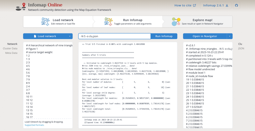
Figure 13: Screenshot of Infomap Online. Infomap Online is a client-side web application that enables users to run Infomap in the web browser. We achieve this by compiling Infomap from C++ to JavaScript and provide a graphical user interface for all input and output parameters. Infomap Online is available at https://www.mapequation.org/infomap/.

Bipartite connectivity parameter.

If the given network has a bipartite structure with $N_{L}$ left nodes and $N_{R}$ right nodes, we adjust the connectivity parameter accordingly: we use the smallest $\lambda^{\text{bi}}$ at which a random bipartite network is almost surely connected [60]

$$\lambda^{\text{bi}}=\frac{\ln\left(N_{L}+N_{R}\right)}{\min\left(N_{L},N_{R}\right)}.$$ (47)

We also adapt the definition of prior link weights to reflect that links in bipartite networks must connect different-type nodes,

$$\gamma_{uv}^{\text{bi}}=\left(1-\delta_{\tau_{u}\tau_{v}}\right)\lambda^{\text{bi}}c_{uv},$$ (48)

where $\tau_{u}$ and $\tau_{v}$ are the types of nodes $u$ and $v$, that is, left or right.

Metadata connectivity parameter.

Nodes annotated with metadata allow further fine-tuning the connectivity parameter. We expect the $N_{\ell}$ nodes with the same metadata label $\ell$ to be connected with higher probability. With metadata labels $\ell_{u}$ and $\ell_{v}$ for nodes $u$ and $v$, we adjust the prior connectivity to

$$\lambda_{uv}^{\text{meta}}=\lambda+\delta_{\ell_{u}\ell_{v}}\lambda_{\ell_{u}},$$ (49)

where $\delta$ is the Kronecker delta, and $\lambda_{\ell_{u}}=\frac{\ln N_{\ell_{u}}}{N_{\ell_{u}}}$.

VIII Software and visualization

Infomap is the search algorithm and a key component of the map equation framework. But to understand the organization of large complex networks, we require both efficient algorithms and powerful visualizations. We have developed several visualization tools with different purposes and made them available as web applications for anyone to use. The first step of community detection with the map equation framework is to install or get access to Infomap.

VIII.1 Infomap

Infomap is the name of the search algorithm that optimizes the map equation. Its core is written in C++ and requires a compiler with C++-14 support.

Python package .

To support the many researchers that use Python for their community detection pipelines, we made Infomap available as a Python package, also called infomap [61]. This package is a small wrapper around the core C++ version of Infomap with additional helper functions and integrates with other popular packages, such as networkx and pandas. A basic version of the package is also included in the popular community detection library CDLib [62].

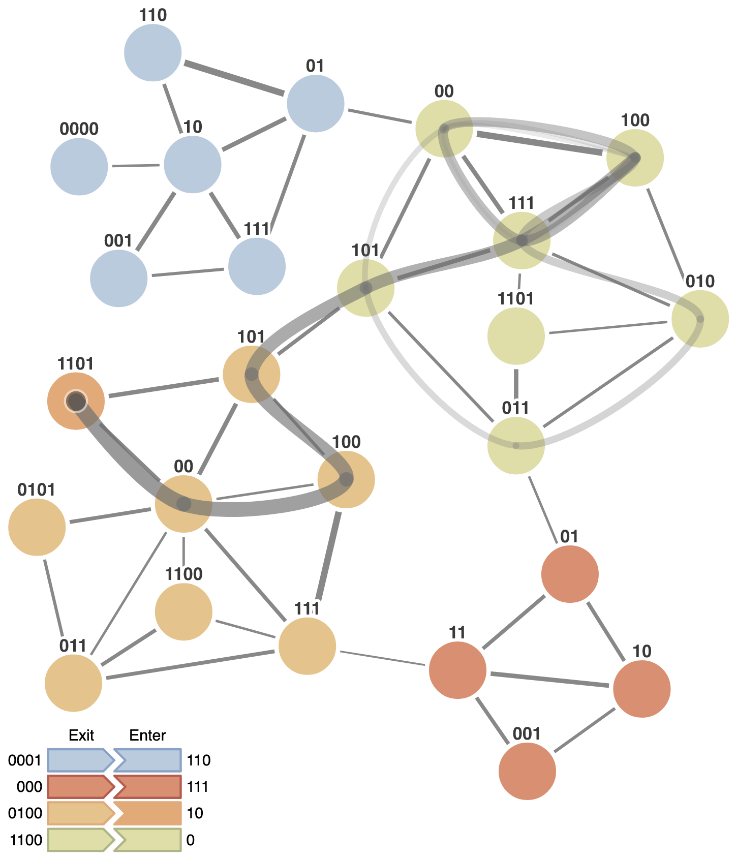
Figure 14: Modular description of a random walk on a network. Each module has its own codebook comprised of node and exit codewords. A global index codebook is comprised of enter codewords for all modules. Each codeword is selected using the Huffman code algorithm on the possible transitions in each codebook.

Infomap Online .

While the most computationally efficient community detection pipeline is to run the stand-alone C++ or Python versions of Infomap, we have embedded a JavaScript version of Infomap into a web application we call Infomap Online (Fig. 13) [63]. This embedded Infomap version supports the same network inputs as C++ Infomap. Infomap Online also serves as interactive documentation for Infomap with examples and simple network visualizations.

VIII.2 Map equation demo 

\begin{overpic}[width=433.62pt]{figures/navigator-schematic.pdf} \put(9.0,2.5){$p_{\mathsf{A}\curvearrowright}$} \put(47.0,2.5){$p_{\mathsf{A}\curvearrowright}p_{\mathsf{AB}}$} \put(86.0,2.5){$p_{\mathsf{B}}^{\circlearrowright}$} \put(47.0,28.0){$p_{\mathsf{B}\curvearrowright}p_{\mathsf{BA}}$} \end{overpic}

Figure 15: Schematic representation of two connected modules. Modules are represented by circles with areas proportional to the contained flow $p_{\mathsf{m}\circlearrowright}$ and border thickness proportional to the exiting flow $p_{\mathsf{m}\curvearrowright}$. Links with thickness and lightness proportional to – and length inversely proportional to – the aggregated flow volume between modules $p_{m\curvearrowright}p_{mn}$.

While the map equation does not depend on explicitly deriving codewords or simulating random walks, visualizing the modular description of a random walk can highlight the mechanics of the map equation. To do this, we have developed a web-based demo application [64]. In this application, we show how modular Huffman codes [65] enable re-using codewords in different modules by encoding module transitions with exit and enter codewords. This enables a shorter expected codelength for partitions where the random walker spends a relatively long time inside modules compared to exiting and entering other modules. In Fig. 14, we show a realization of a random walk starting in the green – top right – module and transitioning to the orange – bottom left – module. Every module transition is encoded using a module-specific exit codeword followed by an enter codeword from the index codebook.

VIII.3 Infomap Network Navigator 

Understanding real-world systems relies on effectively mapping complex networks. To comprehend and navigate the intricate multilevel communities within these networks, it is crucial to employ powerful visualizations that can transform textual representations into visually intuitive maps. To address this need, we have developed an interactive web application called Infomap Network Navigator [66, 67]. This tool allows users to visualize and explore multilevel maps of both conventional and higher-order networks in a manner similar to using mapping software such as Google Maps.

We visualize multilevel communities using top-level modules represented by circles. The circle areas indicate the contained flow volume, while the border thickness represents the exiting flow volume (Fig. 15). Modules are connected by aggregated links, with their thickness and color lightness reflecting the flow between them. Additionally, we adjust the link lengths inversely proportional to the inter-module flow, emphasizing varying connection strengths. Figure 16 illustrates using the Infomap Network Navigator to highlight multilevel citation flow patterns in science.

At the top level, the application visualizes research fields like the life sciences, physical sciences, and social sciences. By zooming in using the mouse wheel or trackpad, more detailed information becomes visible. For example, within the life sciences, the application reveals further divisions into research areas such as molecular biology and medicine.

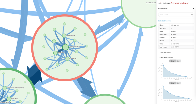
Figure 16: Screenshot of Infomap Network Navigator. The Network Navigator is a web application that generates an interactive zoomable map for networks clustered with Infomap. The citation flow patterns in science are organized in a multilevel partition. Zooming in reveals sub-modules within the life sciences, such as molecular biology and medicine. Modules are represented as in Fig. 15. The Infomap Network Navigator is available at https://www.mapequation.org/navigator/.

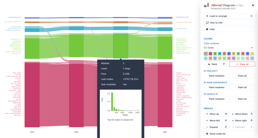
Figure 17: Screenshot of the Alluvial Diagram Generator. Alluvial diagrams visualize how the modular organization of networks changes. Each vertical stack represents the network’s organization, here for journal citation data from different time points. The Alluvial Diagram Generator is available at https://www.mapequation.org/alluvial/.

\begin{overpic}[width=411.93767pt]{figures/modular_schematic.pdf} \put(0.0,69.0){a} \put(63.0,69.0){b} \put(30.0,64.0){{\color[rgb]{0.3828125,0.578125,0.765625}{A}}} \put(27.0,6.0){{\color[rgb]{0.92578125,0.65234375,0.4375}{B}}} \put(6.5,60.0){\footnotesize{\color[rgb]{0.3828125,0.578125,0.765625}I}} \put(54.0,49.0){\footnotesize{\color[rgb]{0.3828125,0.578125,0.765625}II}} \put(1.8,16.6){\footnotesize{\color[rgb]{0.92578125,0.65234375,0.4375}IV}} \put(48.0,16.0){\footnotesize{\color[rgb]{0.92578125,0.65234375,0.4375}III}} \put(63.0,1.0){\footnotesize{Two-level}} \put(86.0,1.0){\footnotesize{Multilevel}} \put(63.1,48.0){\footnotesize{\color[rgb]{0.3828125,0.578125,0.765625}{A}}} \put(63.1,18.0){\footnotesize{\color[rgb]{0.92578125,0.65234375,0.4375}{B}}} \put(99.0,56.0){\footnotesize{\color[rgb]{0.3828125,0.578125,0.765625}I}} \put(99.0,42.0){\footnotesize{\color[rgb]{0.3828125,0.578125,0.765625}II}} \put(99.0,27.0){\footnotesize{\color[rgb]{0.92578125,0.65234375,0.4375}III}} \put(99.0,15.0){\footnotesize{\color[rgb]{0.92578125,0.65234375,0.4375}IV}} \end{overpic}

Figure 18: Schematic alluvial diagram of multilevel network structure. (a) A weighted network with a multilevel modular structure. The two blue and orange top-level modules (A–B) are further divided into two sub-modules each (I–IV), indicated by color lightness. (b) An alluvial diagram representation of the top-level and multilevel modules in (a) using the same colors. Columns of blocks represent modules with heights proportional to the contained flow volume. The leftmost column is an ordinary two-level alluvial diagram representation. The multilevel representation to the right shows multiple levels, with the background showing the top-level organization. Streamfields connect modules in the left and right columns that share nodes.

VIII.4 Alluvial Diagram Generator 

Complex systems, such as social or biological systems, are dynamic. This results in changing interaction patterns over time. Understanding this change is essential to gain insights into the organization and evolution of complex systems.

Various summary statistics can quantify these structural changes, such as variation of information or normalized mutual information, which compute a distance or similarity between two partitions [68, 69, 70, 71]. While these metrics have their use cases, they do not capture essential information about how the networks change.

\begin{overpic}[width=433.62pt]{figures/bioregions-schematics-wrap.pdf} \put(0.0,72.0){a} \put(35.5,72.0){b} \put(79.0,72.0){c} \put(79.0,32.0){d} \put(35.0,32.0){e} \put(0.0,32.0){f} \end{overpic}

Figure 19: Infomap Bioregions. Schematic illustration of bioregional mapping from species distribution data to bioregions. Network-based methods identify bioregions from species distribution data (a) by binning species observations into spatial grid cells (b). Grid cells and species form nodes in a bipartite network where a links indicate species occurrence in grid cells (c). Infomap detects communities (d). In bipartite networks, communities contain grid cells and species; the grid cells assigned to the same community form a bioregion (e). In the interactive Infomap Bioregions tool, available at https://www.mapequation.org/bioregions/, bioregional maps can be exported to various formats (f).

Powerful visualization tools are necessary to effectively visualize and understand how and where these changes occur. Alluvial diagrams visually represent the changing organization of networks by embedding each network’s modules as vertically stacked blocks (Fig. 17) [72, 73]. The height of these blocks is proportional to the flow volume of the nodes they contain. By positioning different networks adjacent to one another and connecting modules with shared nodes using streamfields – the middle part of Fig. 18b – the diagrams highlight the changing organization. To incorporate multilevel solutions in alluvial diagrams, we display hierarchically nested sub-modules above their corresponding super-modules. We illustrate this in the right stack in Fig. 18b.

We developed an alluvial diagram generator as a web application [74] operating within the user’s web browser, ensuring that data is not uploaded or shared with any server. This is crucial for researchers working with sensitive data, as it eliminates the risk of unintentional data sharing with external parties.

IX Applications

The map equation’s coding principles form a sound foundation for community-aware and compression-based node centrality and similarity scores. As an efficient information-theoretic community-detection algorithm, Infomap enables robust relational data applications, including data-driven bioregionalization based on species distributions in biodiversity research and network inference from correlational data in systems biology.

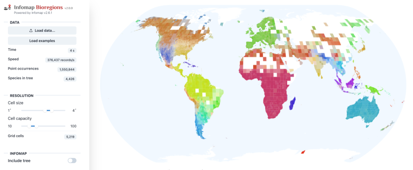
Figure 20: Screenshot of Infomap Bioregions. Infomap Bioregions is a web application for interactive exploration of species distribution data and bioregional patterns. The map shows mammal occurrence distributions where white areas have too few data points to derive statistics. Infomap Bioregions is available at https://www.mapequation.org/bioregions.

IX.1 Map equation centrality 

Node centrality measures characterize how important or influential each node in a network is and often take a local or global perspective, relating node importance, for example, to node degree or the number of shortest paths passing through a node. We can also interpret node flow – the random walker’s stationary visit rates – as a global node importance measure. So-called community-aware centrality measures take a node’s community membership and link patterns to other nodes within and outside their community into account.

To derive a community-aware centrality score from the map equation, we take inspiration from the so-called Vickrey-Clarke-Groves (VCG) principle that provides a way to set item prices in multi-item auctions [75]. The VCG price that a bidder $b$ has to pay for an item $i$ is the collective marginal harm $b$ causes to other bidders who, because of $b$’s existence, receive another item $j\neq i$ which they value lower than $i$. Importantly, $b$’s price for $i$ does not depend on $b$’s wealth because it is “the difference between the optimal valuation achievable by allocating everyone except person $b$ to all the positions and the optimal valuation obtainable by allocating everyone except person $b$ to all positions other than i” [76].

Applying the VCG mechanism to the map equation’s coding principles, and given a partition $\mathsf{M}$, we calculate node $u$’s importance as the codelength difference between assigning codewords to all nodes but never using $u$’s codeword and assigning codewords to all nodes except for $u$, and define map equation centrality [77],

$$\lambda\left(\mathsf{M},u\right)=-\left(p_{\mathsf{m_{u}}}^{\circlearrowright}-p_{u}\right)\log_{2}\frac{p_{\mathsf{m}_{u}}^{\circlearrowright}-p_{u}}{p_{\mathsf{m}_{u}}^{\circlearrowright}},$$ (50)

where $p_{\mathsf{m}_{u}}$ is the module to which $u$ is assigned. In case of the one-level partition $\mathsf{M}_{1}$, map equation centrality simplifies to

$$\lambda\left(\mathsf{M}_{1},u\right)=-\left(1-p_{u}\right)\log_{2}\left(1-p_{u}\right).$$ (51)

Map equation centrality quantifies by how many bits, in total, the codewords for the remaining nodes could be shortened if node $u$ were not present. Because of the map equation’s modular codebook structure, node $u$’s presence, or absence, only affects the codewords for the nodes within $u$’s module. Therefore, $u$’s importance is fully determined by its codeword usage rate and its module’s codebook usage rate.

\begin{overpic}[width=433.62pt]{figures/ModSel_MapEqRev-v2.pdf} \put(0.0,24.0){a} \put(25.0,24.0){b} \put(50.0,24.0){c} \put(75.0,24.0){d} \end{overpic}

Figure 21: Model selection. Module-based regularization finds the best balance between over- and underfitting modular structure to correlational data. The best model is found by measuring the relative codelength savings in the training network with the modules from the test network (Eq. 52) as the regularization parameter $\lambda$ varies (a). Weak regularization leads to conserving many links and underfitting modular structure (b). The maximum codelength savings give the best representation of modular structure in the data (c), enabling the researcher to learn more about the underlying system. Excessive regularization removes many links and overfits modular structure to the data (d). Common regularization methods, using heuristics or maximizing the likelihood of the model, are prone to underfit modular structure, in this way obscuring potentially important insights.

IX.2 Map equation similarity 

Node similarity measures quantify how similar or dissimilar two nodes are and find applications in link-prediction and representation-learning tasks. From a compression perspective, we can quantify how similar node $v$ is to node $u$ by relating it to the required number of bits for encoding a random-walker step from $u$ to $v$. However, while the network constrains what steps a random walker can take, a coding scheme is more flexible: Once we have inferred the community structure of a network and assigned codewords to modules and nodes, we can use the coding scheme to describe transitions between any pair of nodes, whether they are connected or not. Map equation similarity – mapsim for short – takes this approach and derives node similarities from the random walker’s transition rates between nodes and modules [78].

To calculate the similarity $\operatorname{mapsim}\left(u,v,\mathsf{M}\right)$ of node $v$ to node $u$, given a partition $\mathsf{M}$, we find the smallest module $\mathsf{m}\in\mathsf{M}$ that contains both $u$ and $v$. Then, we calculate the rate $r_{u,\mathsf{m}}$ at which a random walker who is at $u$ transitions up to the root level of $\mathsf{m}$, and the rate $r_{\mathsf{m},v}$ at which a random walker who is at the index level of $\mathsf{m}$ transitions to and visits node $v$. By multiplying those two rates, we obtain the rate at which the random walker transitions from $u$ to $v$, $\operatorname{mapsim}\left(u,v,\mathsf{M}\right)=r_{u,\mathsf{m}}r_{\mathsf{m},v}$. We can interpret $\operatorname{mapsim}\left(u,v,\mathsf{M}\right)$ as the distance from $u$ to $v$, in bits, by setting $d_{uv}=\log_{2}\operatorname{mapsim}\left(u,v,\mathsf{M}\right)$.

IX.3 Infomap Bioregions 

In biodiversity research, categorizing ecosystems and identifying the areas most critical for conservation depends on high-quality data-derived biogeographical regions, or simply bioregions. Bioregions reveal how species are grouped at large spatial scales and serve as essential units for understanding historical biogeography, ecology, and evolution.

Network-based methods uncover bioregions from species distribution data by first binning all species into spatial grid cells. All species and grid cells together form a bipartite network where a link indicates the presence of a species in a particular grid cell. Figure 19 shows a schematic illustration of bioregional mapping of species distribution data using Infomap Bioregions [79] and Fig. 20 shows a screenshot of Infomap Bioregions. For example, conservation biologists have used the tool to delineate bioregions in one of our planet’s most biodiverse hotspots, the tropical Andes, to understand the spatial and temporal evolution of the biota [80]. In another study, researchers applied our method to about 25,000 vascular plant species in tropical Africa to determine whether different forms of plant growth display similar diversity patterns [81].

IX.4 Model selection with correlational data 

Correlational data is observed and analyzed in various fields across the sciences. For example, gene co-expression data and species co-occurrence data all have features observed through repeated sampling. This type of data is often represented as correlation networks, where the observed features are the nodes and their respective correlations are the links. These networks can inform the researchers about genes sharing a similar function or about species preferring similar conditions, but they are in general dense and need to be regularized and sparsified to allow for further analysis (Fig. 21). This is a model selection problem where a regularization parameter has to be tuned, and we have suggested a principled way of basing this model selection on modular structure in the underlying data [82], contrasting commonly used methods that rely on ad-hoc heuristics or on conserving relations in the data rather than structure. This should be more intuitive to researchers since they often study modular structure, that is communities, clusters, or groups, in subsequent analyses. Our module-based regularization extends to Gaussian graphical models, where we suggested a module-based graphical lasso to infer a sparse precision matrix from correlational data, with improved performance when the data are noisy [83].

When regularizing the correlation network the code length $L^{\lambda}\left(\mathsf{M}\right)$, with a partition $\mathsf{M}$ of the network, will depend on the regularization parameter $\lambda$, as indicated by the superscript. For model selection through cross-validation, we split the data into a training and a test set and infer the corresponding training and test networks with a specific value of $\lambda$. The model selection criterion we use is to maximize the modular structure in the training network also found in the test network, such that the fraction

$$\frac{L^{\lambda,\mathrm{test}}(\mathsf{1})-L^{\lambda,\mathrm{test}}(\mathsf{M}^{\mathrm{train}})}{L^{\lambda,\mathrm{test}}(\mathsf{1})}$$ (52)

is maximized. This fraction is the relative codelength savings in the test network when we use the modules found in the training network, with $L(\mathsf{1})$ denoting the one-level, uncompressed, codelength, with all nodes in the same module. The best $\lambda$ is thus the value that corresponds to the maximum of this fraction. If we were to fit a polynomial to data and select the degree through cross-validation, the degree expresses the model complexity and is analogous to the modular structure here. Figure 21 shows an example where module-based regularization is applied.

X Conclusion

Simplifying the dynamic processes on networks to uncover how complex systems work remains a challenging problem with many applications. To help researchers take full advantage of the map equation framework and its community-detection algorithm Infomap, we explain the information-theoretical principles of the map equation and summarize its many generalizations to various network representations, flow models, and modular descriptions. As network science advances, flow-based community detection methods will remain essential for unraveling the complexities of networked systems and their inner workings. We hope our review can inspire further generalizations of the map equation to simplify and highlight important dynamic structures in innovative network models.

X.1 Data and code availability

Software is available at https://mapequation.org. Infomap is available at https://mapequation.org/infomap and its source code at https://github.com/mapequation/infomap. Data and notebooks are available at https://github.com/mapequation/infomap-tutorial-notebooks.

X.2 Author contributions

All authors wrote and edited the manuscript.

X.3 Competing interests

The authors declare that they have no competing interests.

- [1] Santo Fortunato. Community detection in graphs. Physics Reports, 486(3):75–174, 2010.
- [2] Santo Fortunato and Darko Hric. Community detection in networks: A user guide. Physics Reports, 659:1–44, 2016.
- [3] Michael T. Schaub, Jean-Charles Delvenne, Martin Rosvall, and Renaud Lambiotte. The many facets of community detection in complex networks. Applied network science, 2(1):1–13, 2017.
- [4] Leto Peel, Daniel B. Larremore, and Aaron Clauset. The ground truth about metadata and community detection in networks. Science advances, 3(5):e1602548, 2017.
- [5] Fan-Yun Sun, Meng Qu, Jordan Hoffmann, Chin-Wei Huang, and Jian Tang. vgraph: A generative model for joint community detection and node representation learning. Advances in Neural Information Processing Systems, 32, 2019.
- [6] Jaewon Yang and Jure Leskovec. Overlapping communities explain core-periphery organization of networks. Proceedings of the IEEE, 102(12):1892–1902, 2014.
- [7] Tiago P. Peixoto. Bayesian Stochastic Blockmodeling, chapter 11, pages 289–332. John Wiley & Sons, Ltd, 2019.
- [8] Andrea Lancichinetti and Santo Fortunato. Community detection algorithms: A comparative analysis. Physical Review E, 80:056117, Nov 2009.
- [9] Rodrigo Aldecoa and Ignacio Marín. Exploring the limits of community detection strategies in complex networks. Scientific Reports, 3:2216, 2013.
- [10] Lovro Šubelj, Nees Jan van Eck, and Ludo Waltman. Clustering scientific publications based on citation relations: A systematic comparison of different methods. PLoS One, 11(4):1–23, 2016.
- [11] Pascal Pons and Matthieu Latapy. Computing Communities in Large Networks Using Random Walks. Journal of Graph Algorithms and Applications, 10:191–218, 2006.
- [12] Jean-Charles Delvenne, Sophia N. Yaliraki, and Mauricio Barahona. Stability of graph communities across time scales. Proceedings of the National Academy of Sciences, 107:12755–12760, 2010.
- [13] Michael T. Schaub, Jean-Charles Delvenne, Sophia N. Yaliraki, and Mauricio Barahona. Markov dynamics as a zooming lens for multiscale community detection: Non clique-like communities and the field-of-view limit. PLoS One, 7(2):1–11, 2012.
- [14] Renaud Lambiotte, Jean-Charles Delvenne, and Mauricio Barahona. Random Walks, Markov Processes and the Multiscale Modular Organization of Complex Networks. IEEE Transactions on Network Science and Engineering, 1:76–90, 2014.
- [15] Martin Rosvall and Carl T. Bergstrom. Maps of random walks on complex networks reveal community structure. Proceedings of the National Academy of Sciences, 105(4):1118–1123, 2008.
- [16] Daniel Edler, Anton Holmgren, and Martin Rosvall. The MapEquation software package. https://mapequation.org, 2022.
- [17] Ludvig Bohlin, Daniel Edler, Andrea Lancichinetti, and Martin Rosvall. Community detection and visualization of networks with the map equation framework. In Measuring scholarly impact, pages 3–34. Springer, 2014.
- [18] Daniel Edler, Ludvig Bohlin, and Martin Rosvall. Mapping Higher-Order Network Flows in Memory and Multilayer Networks with Infomap. Algorithms, 10:112, 2017.
- [19] Gene H. Golub and Charles F. Van Loan. Matrix computations. 3rd edn the johns hopkins university press. Baltimore, MD, 2008.
- [20] David F. Gleich. Pagerank beyond the web. SIAM Review, 57(3):321–363, 2015.
- [21] Renaud Lambiotte and Martin Rosvall. Ranking and clustering of nodes in networks with smart teleportation. Physical Review E, 85:056107, May 2012.
- [22] Jorma Rissanen. Modeling by shortest data description. Automatica, 14(5):465–471, 1978.
- [23] Claude E. Shannon. A mathematical theory of communication. Bell System Technical Journal, 27:379–423, 1948.
- [24] Martin Rosvall and Carl T. Bergstrom. Multilevel Compression of Random Walks on Networks Reveals Hierarchical Organization in Large Integrated Systems. PLoS One, 6:e18209, 2011.
- [25] Tatsuro Kawamoto and Martin Rosvall. Estimating the resolution limit of the map equation in community detection. Physical Review E, 91:012809, 2015.
- [26] Santo Fortunato and Marc Barthélemy. Resolution limit in community detection. Proceedings of the National Academy of Sciences, 104(1):36–41, 2007.
- [27] Tiago P. Peixoto. Parsimonious module inference in large networks. Physical Review Letters, 110:148701, 2013.
- [28] Michael T. Schaub, Renaud Lambiotte, and Mauricio Barahona. Encoding dynamics for multiscale community detection: Markov time sweeping for the map equation. Physical Review E, 86:026112, 2012.
- [29] Masoumeh Kheirkhahzadeh, Andrea Lancichinetti, and Martin Rosvall. Efficient community detection of network flows for varying markov times and bipartite networks. Physical Review E, 93:032309, 2016.
- [30] Daniel Edler, Jelena Smiljanić, Anton Holmgren, Alexandre Antonelli, and Martin Rosvall. Variable markov dynamics as a multifocal lens to map multiscale complex networks. arXiv: 2211.04287, 2022.
- [31] Vincent D. Blondel, Jean-Loup Guillaume, Renaud Lambiotte, and Etienne Lefebvre. Fast unfolding of communities in large networks. Journal of Statistical Mechanics: Theory and Experiment, 2008(10):P10008, 2008.
- [32] Vincent A. Traag, Ludo Waltman, and Nees Jan van Eck. From Louvain to Leiden: guaranteeing well-connected communities. Scientific Reports, 9(1):5233, 2019.
- [33] Christopher Blöcker, Chester Tan, and Ingo Scholtes. The map equation goes neural, 2023.
- [34] Joaquín Calatayud, Rubén Bernardo-Madrid, Magnus Neuman, Alexis Rojas, and Martin Rosvall. Exploring the solution landscape enables more reliable network community detection. Physical Review E, 100:052308, 2019.
- [35] Pablo M. Gleiser and Leon Danon. Community structure in jazz. Advances in Complex Systems, 06(04):565–573, 2003.
- [36] Leland McInnes, John Healy, Nathaniel Saul, and Lukas Großberger. Umap: Uniform manifold approximation and projection. Journal of Open Source Software, 3(29):861, 2018.
- [37] Wayne W. Zachary. An information flow model for conflict and fission in small groups. Journal of Anthropological Research, 33(4):452–473, 1977.
- [38] Federico Battiston, Giulia Cencetti, Iacopo Iacopini, Vito Latora, Maxime Lucas, Alice Patania, Jean-Gabriel Young, and Giovanni Petri. Networks beyond pairwise interactions: Structure and dynamics. Physics Reports, 874:1–92, 2020.
- [39] Leo Torres, Ann S. Blevins, Danielle Bassett, and Tina Eliassi-Rad. The Why, How, and When of Representations for Complex Systems. SIAM Review, 63(3):435–485, 2021.
- [40] Martin Rosvall, Alcides V. Esquivel, Andrea Lancichinetti, Jevin D. West, and Renaud Lambiotte. Memory in network flows and its effects on spreading dynamics and community detection. Nature Communications, 5(1):4630, 2014.
- [41] Christian Persson, Ludvig Bohlin, Daniel Edler, and Martin Rosvall. Maps of sparse markov chains efficiently reveal community structure in network flows with memory. arXiv: 1606.08328, 2016.
- [42] Aditya Grover and Jure Leskovec. node2vec: Scalable Feature Learning for Networks. In Proceedings of the 22nd ACM SIGKDD International Conference on Knowledge Discovery and Data Mining, KDD ’16, pages 855–864. Association for Computing Machinery, 2016.
- [43] Anton Holmgren, Christopher Blöcker, and Martin Rosvall. Mapping biased higher-order walks reveals overlapping communities. arXiv: 2304.05775, 2023.
- [44] Manlio De Domenico, Andrea Lancichinetti, Alex Arenas, and Martin Rosvall. Identifying Modular Flows on Multilayer Networks Reveals Highly Overlapping Organization in Interconnected Systems. Physical Review X, 5(1):011027, 2015.
- [45] Renaud Lambiotte, Martin Rosvall, and Ingo Scholtes. From networks to optimal higher-order models of complex systems. Nature physics, 15(4):313–320, 2019.
- [46] Carmel Farage, Daniel Edler, Anna Eklöf, Martin Rosvall, and Shai Pilosof. Identifying flow modules in ecological networks using Infomap. Methods in Ecology and Evolution, 12(5):778–786, 2021.
- [47] Alexis Rojas, Joaquin Calatayud, Michał Kowalewski, Magnus Neuman, and Martin Rosvall. A multiscale view of the phanerozoic fossil record reveals the three major biotic transitions. Communications Biology, 4(1):309, 2021.
- [48] Ulf Aslak, Martin Rosvall, and Sune Lehmann. Constrained information flows in temporal networks reveal intermittent communities. Physical Review E, 97:062312, 2018.
- [49] Uthsav Chitra and Benjamin Raphael. Random Walks on Hypergraphs with Edge-Dependent Vertex Weights. In Proceedings of the 36th International Conference on Machine Learning, pages 1172–1181. PMLR, 2019.
- [50] Timoteo Carletti, Federico Battiston, Giulia Cencetti, and Duccio Fanelli. Random walks on hypergraphs. Physical Review E, 101(2):022308, 2020.
- [51] Anton Eriksson, Daniel Edler, Alexis Rojas, Manlio de Domenico, and Martin Rosvall. How choosing random-walk model and network representation matters for flow-based community detection in hypergraphs. Communications Physics, 4(1):1–12, 2021.
- [52] Anton Eriksson, Timoteo Carletti, Renaud Lambiotte, Alexis Rojas, and Martin Rosvall. Flow-Based Community Detection in Hypergraphs. In Higher-Order Systems, Understanding Complex Systems, pages 141–161. Springer International Publishing, 2022.
- [53] Christopher Blöcker and Martin Rosvall. Mapping flows on bipartite networks. Physical Review E, 102:052305, 2020.
- [54] Scott Emmons and Peter J. Mucha. Map equation with metadata: Varying the role of attributes in community detection. Physical Review E, 100:022301, 2019.
- [55] Aleix Bassolas, Anton Holmgren, Antoine Marot, Martin Rosvall, and Vincenzo Nicosia. Mapping nonlocal relationships between metadata and network structure with metadata-dependent encoding of random walks. Science Advances, 8(43):eabn7558, 2022.
- [56] Jelena Smiljanić, Christopher Blöcker, Daniel Edler, and Martin Rosvall. Mapping flows on weighted and directed networks with incomplete observations. Journal of Complex Networks, 9(6), 2021.
- [57] Amir Ghasemian, Homa Hosseinmardi, and Aaron Clauset. Evaluating overfit and underfit in models of network community structure. IEEE Transactions on Knowledge and Data Engineering, page 1–1, 2019.
- [58] Jelena Smiljanić, Daniel Edler, and Martin Rosvall. Mapping flows on sparse networks with missing links. Physical Review E, 102:012302, 2020.
- [59] John Palowitch, Shankar Bhamidi, and Andrew B. Nobel. Significance-based community detection in weighted networks. Journal of Machine Learning Research, 18(188):1–48, 2018.
- [60] A. I. Saltykov. The number of components in a random bipartite graph. Discrete Mathematics and Applications, 5(6):515–524, 1995.
- [61] Daniel Edler, Anton Holmgren, and Martin Rosvall. The Infomap Python package. https://mapequation.github.io/infomap/python/, 2020.
- [62] Giulio Rossetti, Letizia Milli, and Rémy Cazabet. Cdlib: a python library to extract, compare and evaluate communities from complex networks. Applied Network Science, 4(1):1–26, 2019.
- [63] Anton Holmgren, Daniel Edler, and Martin Rosvall. Infomap Online. https://mapequation.org/infomap, 2022.
- [64] Anton Holmgren, Daniel Edler, and Martin Rosvall. The Map Equation Demo. https://mapequation.org/demo, 2022.
- [65] David A. Huffman. A Method for the Construction of Minimum-Redundancy Codes. Proceedings of the IRE, 40(9):1098–1101, 1952.
- [66] Anton Holmgren, Daniel Edler, and Martin Rosvall. Infomap Network Navigator. https://mapequation.org/navigator, 2018.
- [67] Anton Eriksson. Interactive visualization of community structure in complex networks. Master’s thesis, Department of Physics, Umeå University, 2018. diva2:1215352.
- [68] Andrea Lancichinetti, Santo Fortunato, and János Kertész. Detecting the overlapping and hierarchical community structure in complex networks. New Journal of Physics, 11(3):033015, 2009.
- [69] Benjamin H. Good, Yves-Alexandre de Montjoye, and Aaron Clauset. Performance of modularity maximization in practical contexts. Physical Review E, 81(4):046106, 2010.
- [70] Alcides Viamontes Esquivel and Martin Rosvall. Comparing network covers using mutual information. arXiv: 1202.0425, 2012.
- [71] Mark E. J. Newman, George T. Cantwell, and Jean-Gabriel Young. Improved mutual information measure for clustering, classification, and community detection. Physical Review E, 101(4):042304, 2020.
- [72] Martin Rosvall and Carl T. Bergstrom. Mapping Change in Large Networks. PLoS One, 5(1):e8694, 2010.
- [73] Anton Holmgren, Daniel Edler, and Martin Rosvall. Mapping change in higher-order networks with multilevel and overlapping communities. Applied Network Science, 8(1):42, 2023.
- [74] Anton Holmgren, Daniel Edler, and Martin Rosvall. The MapEquation Alluvial Diagram Generator. https://mapequation.org/alluvial, 2022.
- [75] William Vickrey. Counterspeculation, auctions, and competitive sealed tenders. The Journal of finance, 16(1):8–37, 1961.
- [76] Herman B. Leonard. Elicitation of honest preferences for the assignment of individuals to positions. Journal of political Economy, 91(3):461–479, 1983.
- [77] Christopher Blöcker, Juan Carlos Nieves, and Martin Rosvall. Map equation centrality: community-aware centrality based on the map equation. Applied Network Science, 7(1):56, 2022.
- [78] Christopher Blöcker, Jelena Smiljanić, Ingo Scholtes, and Martin Rosvall. Similarity-based link prediction from modular compression of network flows. In The First Learning on Graphs Conference, 2022.
- [79] Daniel Edler, Thaís Guedes, Alexander Zizka, Martin Rosvall, and Alexandre Antonelli. Infomap Bioregions: Interactive Mapping of Biogeographical Regions from Species Distributions. Systematic Biology, 66(2):197–204, 2017.
- [80] Nicolas A. Hazzi, Juan Sebastián Moreno, Carolina Ortiz-Movliav, and Rubén Darío Palacio. Biogeographic regions and events of isolation and diversification of the endemic biota of the tropical andes. Proceedings of the National Academy of Sciences, 115(31):7985–7990, 2018.
- [81] Vincent Droissart, Gilles Dauby, Olivier J. Hardy, Vincent Deblauwe, David J. Harris, Steven Janssens, Barbara A. Mackinder, Anne Blach-Overgaard, Bonaventure Sonké, Marc SM Sosef, et al. Beyond trees: Biogeographical regionalization of tropical Africa. Journal of Biogeography, 45(5):1153–1167, 2018.
- [82] Magnus Neuman, Viktor Jonsson, Joaquín Calatayud, and Martin Rosvall. Cross-validation of correlation networks using modular structure. Applied Network Science, 7(1):75, 2022.
- [83] Magnus Neuman, Joaquín Calatayud, Viktor Tasselius, and Martin Rosvall. Module-based regularization improves gaussian graphical models when observing noisy data. arXiv:2303.16796, 2023.