Impact of HPO on AutoML Forecasting Ensembles

Abstract

A forecasting ensemble consisting of a diverse range of estimators for both local and global univariate forecasting, in particular MQ-CNN [1], DeepAR [2], Prophet [3], NPTS, ARIMA and ETS [4], can be used to make forecasts for a variety of problems. This paper delves into the aspect of adding different hyperparameter optimization strategies to the deep learning models in such a setup (DeepAR and MQ-CNN), exploring the trade-off between added training cost and the increase in accuracy for different configurations. It shows that in such a setup, adding hyperparameter optimization can lead to performance improvements, with the final setup having a 9.9 % percent accuracy improvement with respect to the avg-wQL over the baseline ensemble without Hyperparameter Optimisation (HPO), accompanied by a 65.8 % increase in end-to-end ensemble latency. This improvement is based on an empirical analysis of combining the ensemble pipeline with different tuning strategies, namely Bayesian Optimisation and Hyperband and different configurations of those strategies. In the final configuration, the proposed combination of ensemble learning and HPO outperforms the state of the art commercial AutoML forecasting solution, Amazon Forecast, with a 3.5 % lower error and 16.0 % lower end-to-end ensemble latency.

Keywords AutoML  $\cdot$ Forecasting  $\cdot$ Ensemble Learning  $\cdot$ Hyperparameter Tuning

1 Introduction

1.1 Motivation

There is a wide range of possible applications for forecasting algorithms, making it hard to find a single model that performs well on all of them. Due to this uncertainty over which models will perform best, it is common place in the forecasting space that domain experts and data scientists have to experiment with several methods before they find one that works acceptably well on a particular problem. This exploration process can be time and resource consuming and is not always practical, due to the plethora of unsolved forecasting problems as well as the scarcity of domain experts and data scientists.

In recent years, Automated Machine Learning (AutoML) has become more popular, allowing non-technical users to solve machine learning problems without in depth knowledge about the underlying methodology, filling in for the lack of available data scientists through automation [5]. In forecasting there are several approaches to AutoML, one of them being the established method of using ensemble learning and aggregation of forecasts [6]. This has seen a recent increase in attention, with the top performing models in the M4 Competition [7] being of this nature [8].
Ensembling, can be conceptualised as the automation of the previously manual step of exploring the performance of various algorithms on a given problem and selecting the best one or a combination of models. This, however, does not address another important aspect of data science which is the selection of good hyperparameters, leading to better performance of a model trained using a particular algorithm. The combination of ensemble learning and hyperparameter tuning in an AutoML forecasting setup will be discussed in this paper.

Specifically, the paper concerns itself with the question whether hyperparameter optimisation adds accuracy improvements to a forecast ensemble (as described in section 5) and if the corresponding latency increase is justifiable from a business perspective. It further delves into the evaluation of different tuning strategies, such as Bayesian Optimisation and Hyperband, in different variations to find an optimal configuration.

To provide the necessary background for answering the scientific question, the paper will first outline the methods used as part of the research underlying this paper, focusing on the forecasting algorithms that are part of the ensemble, the different hyperparameter tuning strategies that were tested and finally, the ensemble strategy employed. The experiments that are part of this paper, combine the described methods into an end-to-end AutoML pipeline for forecasting, that can be parameterised to run the necessary configurations for different experiments. This setup is outlined in subsection 5.2. To ensure more rigorous results, all experiments were repeated on four different datasets, namely Covid Death [9], Solar [10], Electricity [11] and Kaggle retail [12], the properties of which and why they were chosen is outlined in section 4.
Chapter 5 is the core of this paper, both analysing and evaluating experiments and their findings. It first explores the accuracy and latency effect of adding hyperparameter optimisation to individual, deep-learning-based algorithms, which is discussed in subsection 5.1. With the knowledge gained from these first exploratory steps, subsection 5.3 will detail how the changes in performance of these individual algorithms translates to the effects on the output of the ensemble. A direct comparison between the two different tuning strategies, Hyperband and Bayesian Optimisation, is part of subsection 5.5 and a more detailed analysis of the winning strategy (Hyperband) is part of subsection 5.6, which will compare different variations of set strategy as part of the ensemble.

1.2 Background

This section contains a general introduction to forecasting and provides an overview of related work on the subject of AutoML ensemble forecasting.

At the root of every forecasting problem lies the intent to gather intelligence about the occurrence of a future event. In the context of time series forecasting, this means generating a prediction about the behaviour of events in the future, building on the premise that one can use past information to make inferences about the future. Machine Learning and Statistics make use of (learned) models to find patterns in time series data and use them to generate a forecast about the future.
Forecasting problems can be differentiated as univariate and multivariate. In the former, the model used considers the past observations of a single time series to build a forecast for it. Whereas in multivariate forecasting, the model uses past observations of multiple time series to forecast those same time series [13].
Furthermore, forecasting problems can be divided into local and global ones. Where the previous distinction between univariate and multivariate aimed at differentiating based on the number of time series utilised at inference time, the difference between local and global problems is determined during model formation. The parameters $\mathbf{\theta}$ of a local model are estimated on the target time series, meaning the time series one wants to forecast. This approach works well if a sufficient number of past observations in the target time series exists, to train the model. If this is not the case, it makes sense to consider the assumption that similar or related time series could improve performance. This is then called a global model, for which the parameters $\theta$ are estimated on a body of related time series (as well as the target time series) [14].
The two aforementioned categorisations aim at distinguishing based on the variables used. To introduce the aspect of certainty into the resulting forecast, one has to differentiate between point-forecasts and probabilistic models. A point forecast outputs a single value estimate for each predicted time step, according to a given metric. Whilst this makes it easier to interpret the forecast, it fails to give a sense of certainty about the prediction. Probabilistic forecasting models yield a probability distribution for each time step which provides a quantifiable way of measuring the uncertainty of the model output. These different classes of forecasting problems can be combined, leading to the categorisation in Table 1.

Forecast Type	Model Type	Formulation
Point	Local univariate	$\hat{\mathbf{z}}_{i,t+1:t+1}=\Psi(\mathbf{z}_{i,1:t},\mathbf{X}_{i,1:t+1})$
	Global univariate	$\hat{\mathbf{z}}_{i,t+1:t+1}=\Psi(\mathbf{z}_{i,1:t},\mathbf{X}_{i,1:t+1},\Phi)$
	Local Multivariate	$\hat{\mathbf{Z}}_{i,t+1:t+1}=\Psi(\mathbf{Z}_{i,1:t},\mathbf{X}_{i,1:t+1})$
	Global Multivariate	$\hat{\mathbf{Z}}_{i,t+1:t+1}=\Psi(\mathbf{Z}_{i,1:t},\mathbf{X}_{i,1:t+1},\Phi)$
Probabilistic	Local univariate	$P(\mathbf{z}_{i,t+1:t+1}|\mathbf{z}_{i,1:t},\mathbf{X}_{i,1:t+1};\theta_{i})$, $\theta_{i}=\Psi(\mathbf{z}_{i,1:t},\mathbf{X}_{i,1:t+1})$
	Global univariate	$P(\mathbf{z}_{i,t+1:t+1}|\mathbf{z}_{1:t},\mathbf{X}_{1:t+1};\theta_{i})$, $\theta_{i}=\Psi(\mathbf{z}_{i,1:t},\mathbf{X}_{i,1:t+1},\Phi)$
	Local Multivariate	$P(\mathbf{z}_{i,t+1:t+1}|\mathbf{Z}_{1:t},\mathbf{X}_{1:t+1};\theta_{i})$, $\theta_{i}=\Psi(\mathbf{z}_{i,1:t},\mathbf{X}_{i,1:t+1})$
	Global Multivariate	$P(\mathbf{Z}_{t+1:t+1}|\mathbf{Z}_{1:t},\mathbf{X}_{1:t+1};\theta)$, $\theta=\Psi(\mathbf{Z}_{1:t},\mathbf{X}_{1:t+1},\Phi)$

Let $\mathbf{Z}$ be a set of $n$ univariate time series, where $\mathbf{z}_{i,1:T_{i}}$ is the $i$th series, with observations $z_{i,1}$ to $z_{i,T_{i}}$. $\mathbf{Z}_{t_{1}:t_{2}}$ are the values of all $n$ time series for the time slice $[t_{1},t_{2}]$. The associated set of exogenous covariate vectors is denoted by $\mathbf{X}$. These can include related both dynamic and static features. $\Psi$ maps input features to a probabilistic model, parameterised by $\theta$. The parameters learned from the set of input time series are described by $\Phi$.

Table 1: Forecast Categorisation Overview based on [15]

Ensemble learning can then be used to combine multiple forecasting algorithms to make a single prediction. Ideally, this should be done with a set of algorithms that have diverse strengths (and weaknesses), following the notion that a good ensemble strategy can determine weak spots of one algorithm and cover for them with the strengths of another one. This is not possible when very similar algorithms are chosen, which all have the same strengths and weaknesses.
This paper uses an ensemble based on both local and global, statistical and deep-learning-based models and proposes adding hyperparameter optimisation to the latter ones to improve ensemble accuracy. To the best of my knowledge, this is the first work proposing the specific combination of ensemble learning and forecasting described in section 5.

However, similar work has already been conducted as part of several papers, such as [16][17] and [18]. The former suggest a novel approach for the joint optimisation of neural architecture and hyperparameters of the entire data processing pipeline. In particular, they propose the use of Bayesian Optimisation to jointly optimize different deep-learning-based architectures as well as other pipeline configuration hyperparameters. This technique allowed them to beat multiple well-known traditional statistical models and modern deep-learning models. Their ensemble does, however, only include a set of deep-learning-based models, disregarding possible advantages of traditional statistical forecasting models like Autoregressive Integrated Moving Average (ARIMA) or Exponential Smoothing Algorithm (ETS). Furthermore, they only compare the accuracy of the resulting model, disregarding the practical importance of latency. This may be relevant from a business perspective, since a large search space, as suggested by [16] leads to high latency.
A different approach for AutoML forecasting is suggested by [17], who propose utilising hierarchy-guided model selection, addressing the problem of over fitting, in the context of time series cross validation (sequentially splitting a time series into training and validation partitions). To be precise, they leverage the hierarchical nature which often occurs in time series, by tuning hyperparameters for low level models at a higher level in the data hierarchy. A comprehensive example of this could be the problem of forecasting demand for deserts in the cafeteria of the Cooperative State University Baden-Wuerttemberg Mannheim, with sparse time series (items) for each individual type of desert on a daily basis. In the setting proposed by [17], hyperparameters for models on the desert type basis (lowest level of the data hierarchy) would be tuned on an aggregation of these time series (e.g. by aggregating to a weekly frequency, aggregating to overall desert demand on a daily basis, or a combination of the two), allowing for more general hyperparameters and a potentially better prediction.
Yet another variation is proposed by [18]. They formulate the problem of selecting a good forecasting method as a meta-learning problem, with the goal of selecting a single best model in a way that minimizes the extensive evaluation effort associated with training a multitude of models as done in HPO. As the approach used by [18] is different from the techniques used in this paper, their methods will not be further discussed here.

1.3 Contributions

This Paper proposes the use of HPO in an elaborate AutoML ensemble as outlined in section 5. It provides a detailed empirical analysis and evaluation of the impact of different tuning strategies and configurations on the ensemble pipeline. The experiments conducted as part of this research led to the following primary contributions:

• The paper shows that the Hyperband tuning strategy is generally preferable over Bayesian Optimisation in a AutoML forecast ensemble such as the one used in this paper, with Hyperband on average leading to both a 3.1 % lower error and a 32.7 % lower HPO latency compared to Bayesian Optimisation. A detailed explanation of the experiment design and results can be found in subsection 5.5.

• Results from the experiments in subsection 5.6 show that optimising the configuration of the Hyperband hyperparameter tuning strategy can lead to further improvements in accuracy up to 9.9 % over the baseline without HPO. The paper points out that this improvement in accuracy is associated with a trade-off between error and latency. It provides an analysis of different variations of such a trade-off, pointing out good configurations for a bias toward low latency as well as low error.

• Lastly, the paper suggests a way of finding the optimal strategy and configuration for any given bias between latency and error in subsection 5.6. It proposes tools for both a visual (Figure 16) and an analytical method (Equation 17) of determining such a configuration for a AutoML forecast ensemble.

• Using the optimal strategy and configurations (with the trade-off biased toward accuracy, rather than latency), namely Hyperband with a total number of 30 training jobs for tuning, the AutoML forecast ensemble pipeline outperforms the state of the art commercial AutoML forecasting solution Amazon forecast [19], with a 3.5 % lower error and 16.0 % lower latency.

The paper also includes a comprehensive introduction to forecasting, detailing basic terminology. It further introduces all components of the custom AutoML forecast ensemble used. This includes the forecasting algorithms, an introduction to HPO with a focus on Bayesian Optimisation and Hyperband, as well as an overview of how ensemble learning can be used in the context of forecasting. The paper also outlines the workings of the custom forecast ensemble used in section 5.

2 Methodology

2.1 Forecasting Algorithms

The empirical analysis in this paper is based on six forecasting methods. In particular ARIMA [20], ETS [4], Non-Parametric Time Series Algorithm (NPTS) [21], Prophet [3], Multi-Horizon Quantile Convolutional Neural Network (MQ-CNN) [1] and Autoregressive Recurrent Networks (DeepAR) [2]. This chapter will outline the way these algorithms work, assuming existing knowledge of the fundamental principles of machine learning.

ARIMA is a generalisation of the statistical forecasting model Autoregressive Moving Average (ARMA), which itself is comprised of an autoregressive and a moving average model. Statistical autoregressive (AR) models are based on the assumption that future values can be modeled as a linear combination of past values of the same time series (from Ancient Greek autós means self). As such, an autoregressor is a point local univariate model which depends on the time series $z$ being stationary. This means that $E(\mathbf{z})$ and $Var(\mathbf{z})$ are constant and $\mathbf{z}$ has no seasonality (predictable, periodic behaviour over time). The autoregressor with order $p$, $AR(p)$ is given by Equation 1.

$$\hat{z}_{t+1}=\theta_{0}+\theta_{1}z_{t}+\theta_{2}z_{t-1}+...+\theta_{p}z_{t-p+1}$$ (1)

The order $p$ determines the number of lags (previous time steps taken into account) and the parameter vector $\bm{\theta}$ can be derived from the Partial Autocorrelation Function (PACF) which determines the correlation of $z_{t+1}$ with $z_{t-r}\forall r\in[0,p]$, adjusted for all time steps between $t+1$ and $t-r$ ($z_{t:t-r+1}$). This means that one only cares about the direct effect of $z_{t-r}$ on $z_{t+1}$.
The second part of the ARMA is a moving average model which is also a point local univariate model. It assumes stationary as well and is a function of the constant mean $\mu$ of $\mathbf{z}$ and the error of past observations. The estimator for a moving average model of order $q$ is given by Equation 2.

$$\hat{z}_{t+1}=\mu+\theta_{0}\epsilon_{t}+\theta_{1}\epsilon_{t-1}+...+\theta_{q}\epsilon_{t-q}$$ (2)

With $\epsilon_{i}$ being the error between the estimate $\hat{z}_{i}$ of a past observation and its actual value $\hat{z}_{i}$, $q$ determining the number of past observations taken into account ($\epsilon_{t:t-q}$), and $\bm{\theta}$ being the associated weight vector. The intuition behind the moving average is that if the scalar product of $\bm{\theta}$ and $\bm{\epsilon}$, given by $\bm{\theta}\cdot\bm{\epsilon}$ is positive, this means that the values for the past $q$ time steps $t$ were to low, and so the prediction is increased above the mean, by $\bm{\theta}\cdot\bm{\epsilon}$.
The ARMA model is a linear combination of an autoregressive and a moving average model. As such, it also requires stationarity. The formula for an ARMA model with arguments p and q, ARMA(p,q) is given by Equation 3.

$$\hat{z}_{t+1}=\theta_{0}+\theta_{1}z_{t}+...+\theta_{p}z_{t-p+1}+\mu+\theta_{p+1}\epsilon_{t}+...+\theta_{p+q+1}\epsilon_{t-q}$$ (3)

One of the disadvantages of ARMA is that it requires a constant mean. ARIMA is a generalization of ARMA that also supports time series with a trend ($E(\mathbf{z})\not=\mu$). This is achieved by including a transform from a time series $\mathbf{z}$ with a trend, to a stationary time series $\mathbf{\tilde{z}}$. This transform is called integration, hence the ’I’ in ARIMA. One order of this integration is computed by $\tilde{z}^{(1)}_{t}=z_{t+1}-z_{t}$. To achieve the general case, a third argument, $d$ is introduced, which determines the order of the transform. This is best understood by considering a concrete example: If the order $d$ equals 2, then the transform is applied again to $\tilde{z}^{(1)}_{t}$ yielding $\tilde{z}^{(2)}_{t}$. For the order $d$ this is repeated recursively, resulting in $\tilde{z}^{(d)}_{t}$, which is stationary. ARMA is applied to $\tilde{z}^{(d)}_{t}$ and the reverse of the transform is then computed for the resulting prediction, using $\hat{z}_{t+1}=\sum^{k-l}_{i=0}(z^{(d)}_{t-i})+z_{t}$. For further details about the ARIMA model, refer to [20].

ETS as introduced in [4] is a local univariate time series forecasting method which is based on the notion that a future time step can be estimated as a weighted sum of past observations using smoothing. This requires the time series $\mathbf{z}$ to be stationary. In opposition to regression where one uses all past values at once to fit a model, smoothing recursively computes intermediate predictions, using Equation 4. In ETS this leads to geometrically decreasing weights, assigning lesser importance to older observations, as described in Equation 4.

$$\hat{z}_{t+1}=\hat{z}_{t}+\theta(z_{t}-\hat{z}_{t})$$ (4)

With $\hat{z}_{1}=z_{0}$ and $\theta\in[0,1]$. For $\theta\rightarrow 0$ the model puts a high emphasis on historical values, in particular $\hat{z}_{t+1}=z_{0}|\theta=0$ and for $\theta\rightarrow 1$ the model puts a higher emphasis on recent observation, with the extreme of $\hat{z}_{t+1}=z_{t}|\theta=1$. As discussed by [22], there also exist variation of ETS which adjust for trend and seasonality.

NPTS: Standard parametric methods estimate the parameters of a specified distribution, for example using Maximum Likelihood Estimation (MLE) [23]. These methods may not be efficient and/or consistent when the underlying parametric model does not match the distribution of the data. Contrastingly, non-parametric methods in forecasting have the aim of estimating quantities future time steps such as moments or density directly from past observations without fitting the parameters of a fixed distribution [21]. NPTS method used predicts a probability distribution for future time steps, for each time series individually, making it a probabilistic local univariate model. The statistical estimation is based on a sample taken from past observations, which can be done with different linear and non-linear methods, the former can be expressed using a kernel function and will be the focus of this section. One can further distinguish non-parametric methods for forecasting into autoregressive problems and regression with correlated errors. The former refers to the prediction of a future time step $z_{t+1}$ based on past observations of $\mathbf{z}$ and the latter to predicting $z_{t+1}$ based on observations of the exogenous variable $\mathbf{x}$. The autoregressive estimation of the first and second moment is given by Formula 5.

$$\hat{\mu}_{\mathbf{z},t+1}=E(\mathbf{z}_{t+1}|\mathbf{z}_{1:t}),\;\;\;\hat{\sigma}^{2}_{\mathbf{z},t+1}=Var(\mathbf{z}_{t+1}|\mathbf{z}_{1:t})$$ (5)

The experiments described in section 5 use a kernel with exponential weight decay. This means that observations closer to the current time step are sampled with a higher probability than those further in the past. The kernel $K$ is given by $K(u)=\alpha\cdot e^{-\lambda\cdot|u|}$, where $\alpha$ is the scaling factor, controlling that $\int K(u)\,du=1$ and $\lambda$ being the influencing the rate of weight decay. The explicit density estimator for this case is given by Equation 6.

$$\hat{f}(z_{t+1}|{t+1})=\frac{1}{th}\sum_{i=1}^{t}K\left(\frac{y_{t+1}-y_{i}}{h}\right)$$ (6)

With $t$ being the number of historical observations in the time series and $h$ the bandwidth parameter which controls the width of the kernel window.

Prophet: The prophet model, as introduced by [3] is a probabilistic univariate curve fitting model, that aims at providing a flexible and interpretable basis for forecasting. Prophet consists of three major components: the trend function $g(t)$ representing non-periodic changes over time, seasonality $s(t)$ modeling periodic behaviour of different frequencies, and holidays $h(t)$ for irregularly occurring events.
The trend component $g(t)$ contains two variations: a saturating growth model, and a piecewise linear model. The latter is used for modeling and forecasting saturated growth as it typically occurs for a population in natural ecosystems. A simple form of $g(t)$ as a logistic growth model is given by $g(t)=\frac{C}{1+\exp(-k\cdot(t-m))}$, with $C$ being the carrying capacity (meaning the value toward which the growth converges), $k$ being the growth rate and $m$ the offset parameter. To make this approximation adaptable to a changing carrying capacity and alternating growth rate, [3] suggest making both of them a function of time leading to Equation 7.

$$g(t)=\frac{C(t)}{1+\exp(-(k+\mathbf{a}(t)^{T}\bm{\delta})\cdot(t-(m+\mathbf{a}(t)^{T}\bm{\gamma})))}$$ (7)

Here $C(t)$ denotes the carrying capacity dependent on time and $\bm{\delta}\in\mathbb{R}^{S}$ being a vector of $S$ growth rate adjustments. These changepoints are incrementally activated by computing the scalar of $\bm{\delta}$ and $\mathbf{a}(t)\in\{0,1\}^{S}$, with $\mathbf{a}_{j}(t)=1$ if $t\leq s_{j}$. The changepoints $s_{j}$ can be either manually or automatically selected. Furthermore, the offset $m$ must be adjusted to control for the changing growth rate. This is done by replacing $m$ with $m+\mathbf{a}(t)^{T}\bm{\gamma}$, where $\bm{\gamma}$ is given by Equation 8.

$$\gamma_{j}=\Big{(}s_{j}-m-\sum_{l<j}\gamma_{l}\Big{)}\Big{(}1-\frac{k+\sum_{l<j}\delta_{l}}{k+\sum_{l\leq j}\delta_{l}}\Big{)}$$ (8)

The piecewise linear model can be generally used to represent growth where it is not saturated. It can be conceptualised as breaking a non-linear problem down into multiple stages, so that each can be linearly modeled. These stages are separated by breakpoints which are represented using the growth rate adjustment vector $\mathbf{a}_{j}(t)$. This leads to $g(t)=(k+\mathbf{a}(t)^{T}\bm{\delta})t+(m+\mathbf{a}(t)^{T}\bm{\gamma})$, where $\gamma_{j}=s_{j}\delta$, yields a continuous function. For both trend models, the existence of future changepoints can be simulated based on information from past changepoints.

The seasonality in Prophet, which models periodically reoccurring patterns in the time series with different frequencies, is realized using a standard Fourier series [24]. The concept of which is, to use the sum of trigonometric functions to approximate a well-behaved function. Hence, the seasonal component $s(t)$ is given by $\sum_{n=1}^{N}(a_{n}cos(\frac{2\pi nt}{P})+b_{n}cos(\frac{2\pi nt}{P}))$ and parameterized by $\bm{\theta}=\{a_{1},b_{1},...,a_{N},b_{N}\}$.

Holidays and irregularly occurring events $i$ are modeled using a vector of indicator functions $Z(t)$ (one for each Holiday) that returns $1$ if $t$ is an element of the set of past and future dates of the event $D_{i}$ ($Z(t)=[\mathbf{1}_{t\in D_{1}},..,\mathbf{1}_{t\in D_{L}}]$). The vector $\bm{\kappa}$ contains the the changes to the forecast for the respective holidays, with $\kappa_{i}$ being the forecast shift for event $i$, such that $h(t)=Z(t)\bm{\kappa}$.
The final forecast is then computed as the sum of trend, seasonality and events, as in Equation 9, using posterior sampling making the forecast probabilistic.

$$\hat{z}(t+1)=g(t+1)+s(t+1)+h(t+1)$$ (9)

MQ-CNN as introduced by [1], is a probabilistic forecasting model which is trained on a set of time series to predict a single target time series, making it a global univariate model. Furthermore, it is a Sequence to Sequence (Seq2Seq) model based on a Convolutional Neural Network (CNN) encoder and a Multi Layer Perceptron (MLP) decoder, yielding Multi-horizon Quantile forecasts. These concepts are detailed in the following.
A Seq2Seq model is a model which takes a sequence such as natural language or a time series as an input to compute an outputs sequence. Some of the previously outlined models, namely ARIMA, ETS and NPTS interactively forecast a single next value $z_{t+1}$. They do this recursively until a forecast with the length $K$ of the desired forecasting horizon is generated, which leads to the accumulation errors from previous single steps. However, in Muli-horizon forecasting, the model directly predicts multiple steps $(z_{t+1},...,z_{t+k})$. As suggested by [25] this leads to avoidance of error accumulation whilst retaining efficiency through sharing parameters, making it preferable over single step forecasting.
Like NPTS, Quantile regression is a non-parametric method for capturing the distribution of a time series. It estimates the conditional quantiles of the target $P(z_{t+k}<z^{(q)}_{t+k}|z_{1:t})$, leading to a robust, accurate forecast with sharp prediction intervals [26]. This type of forecast, produces an output matrix $\hat{\mathbf{Z}}=[\hat{z}^{(q)}_{t+k}]_{k,q}\in\mathbb{R}^{Q\times K}$ ($Q$ being the number of predicted quantiles and $K$ the number of horizons/predicted time steps). The respective model is trained using a quantile loss function, such as the total quantile loss, given by $\sum_{t}\sum_{q}\sum_{k}L_{q}(z_{t+k},\hat{z}^{(q)}_{t+k})$.

The primary focus of [26] is a Multi-horizon Quantile Recurrent Forecaster (MQ-RNN). However the paper also suggests that the MQ-framework works with any neural network that has a sequential or temporal structure and is compatible with forking-sequences, such as WaveNet [27]. In the experiments described in this paper, WaveNet, which is a hierarchical causal convolutional network, is used as the encoder, hence MQ-CNN. This encoder outputs hidden states $h_{t}$ for all past observations, which then serve as input for the forked (two branch) MLP decoder. The decoder consists of a global branch $m_{G}(\cdot)$ and a local branch $m_{L}(\cdot)$. The former takes the aforementioned hidden states and future inputs from exogenous covariate vectors $\mathbf{x}^{(f)}_{t:,i}\in\mathbf{X}$ (which is here comprised of past $\mathbf{x}^{(h)}_{:t,i}$, future $\mathbf{x}^{(f)}_{t:,i}$ and static $\mathbf{x}^{(s)}_{i}$ covariate features) to compute a series of horizon-specific contexts $c_{t+1},...,c_{t+K}$ as well as a horizon-agnostic context $c_{a}$, as formalized in Equation 10 (a).

$$(a)\;m_{G}(h_{t},x^{(f)}_{t:})=(c_{t+1},...,c_{t+K},c_{a});\;\;(b)\;m_{L}(c_{t+k},c_{a},x^{(f)}_{t+k})=(\hat{z}^{(q_{1})}_{t+k},...,\hat{z}^{(q_{Q})}_{t+k})$$ (10)

The local MLP is then applied for each time step that is predicted, yielding the final forecast. It computes the output quantiles for each time step based on the corresponding future input and the two contexts from the global MLP as formalized in Equation 10 (b).

DeepAR [2] is a deep-learning-based autoregressive probabilistic global univariate forecasting model, which is based on a Long Short-Term Memory (LSTM) model. A LSTM [28][29] is a modification of a standard Recurrent Neural Network (RNN) that deals with the vanishing or exploding gradient problem (information from some hidden state $h_{n}$ has a exploding or vanishing effect on a later hidden state $h_{n+m}$, depending on the weights of the network, making it difficult for the network to detect the relevant signal). It does this by introducing the cell state, which has the purpose of capturing useful long-term information, and three gates: the forget-gate, the input-gate and the output-gate, which each represent an attention mechanism (here weight matrix) that determines relevant information. The forget gate calculates a weight matrix $f_{t}$ with the relevance of information from the previous cell state $c_{t-1}$. The input gate calculates a similar weight matrix for the preliminary current cell state $\tilde{c}_{t}$. The current cell state $c_{t}$ is then computed as $f_{t}\odot c_{t-1}+i_{t}\odot\tilde{c}_{t}$ (with $\odot$ denoting element-wise matrix multiplication), essentially making $c_{t}$ a combination of previous and current relevant information. The output gate $o_{t}$ is computed to determine what information of $c_{t}$ is relevant to the current hidden state $h_{t}$, which is then calculated as a function of $o_{t}$ and $c_{t}$. The computation in a single LSTM cell can be visualized as in Figure 1.

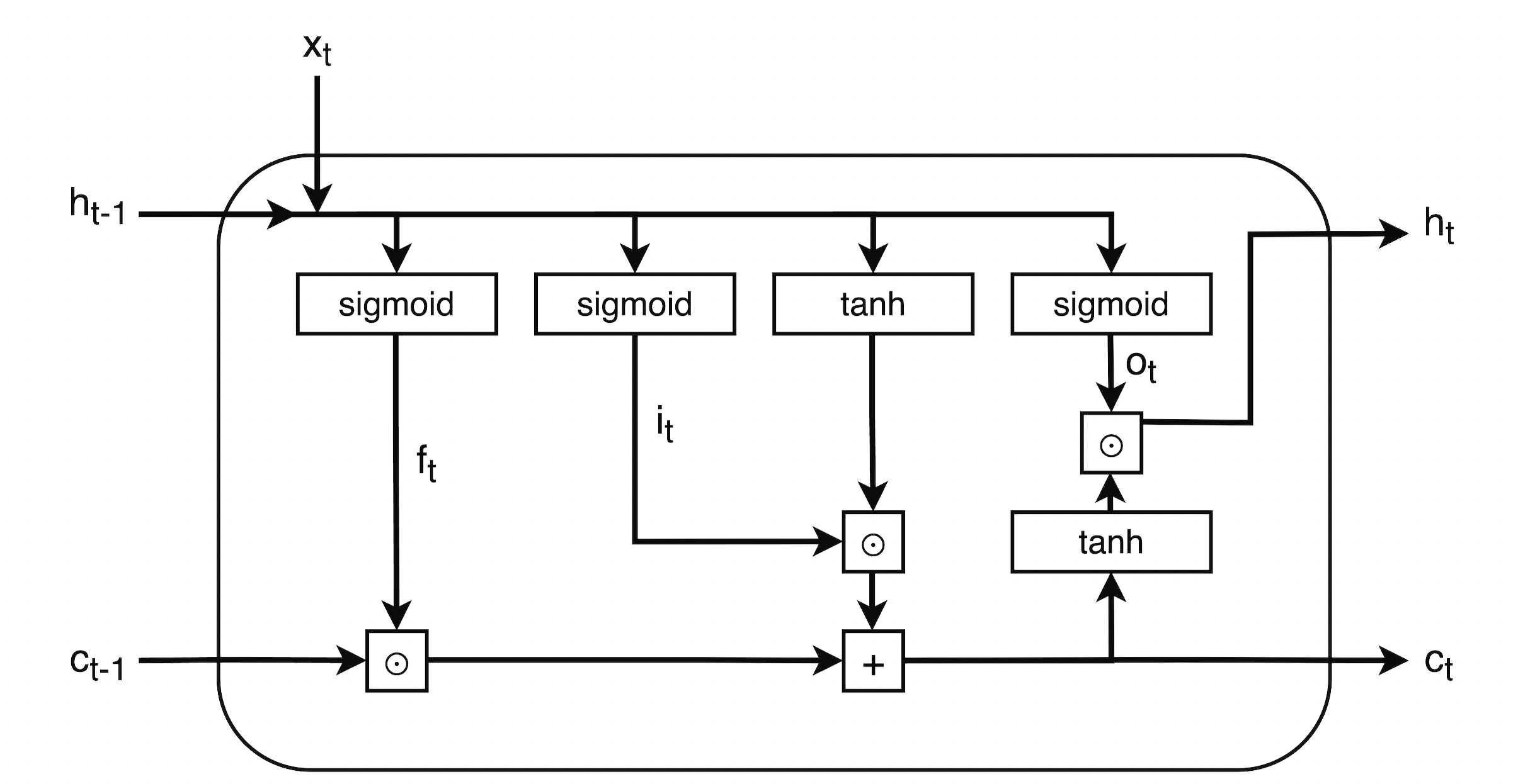
Figure 1: Computation in a single LSTM cell

DeepAR uses such an LSTM for both the conditioning (encoder) range, in which the model recursively takes in observations from past time steps, and in the prediction (decoder) range, where the model continues to unroll predicting the distribution of future time steps as given by

$$P(\mathbf{z}_{i,t+1:t+K}|\mathbf{z}_{1:t},\mathbf{x}_{1:t+1})$$ (11)

According to [2] DeepAR performs particularly well when provided with large amounts of related and covariate time series, it offers the advantages of minimal manual intervention by experts, due to the fact that seasonal behaviors and dependencies on given covariates across time series are automatically modelled. It further provides the ability to compute forecasts for time series with few or no past observations, as long as they are related to the time series the model was trained on.

2.2 Algorithm Evaluation

In the empirical evaluation described in section 5 the aforementioned algorithms and the resulting ensemble are evaluated using a set of metrics, namely: Mean Absolute Percentage Error (MAPE), Mean Absolute Scaled Error (MASE), Weighted Absolute Percentage Error (WAPE) and wQL. In the following section, these metrics are described in more detail.
MAPE is an average over the absolute percentage error between predicted and true values for each time step. It is particularly useful if the time series has a high variance, with outliers having a higher impact. MAPE can be computed as shown in Equation 12, with $n$ being the number of time steps, $z_{t}$ the observed value at time step $t$ and $\hat{z}_{t}$ being the forecasted value at $t$.

$$MAPE=\frac{1}{n}\sum^{n}_{t=1}|\frac{z_{t}-\hat{z}_{t}}{z_{t}}|$$ (12)

MASE is a scaled version of the Mean Absolute Error (MAE). The scaling factor is the MAE of the naive forecast method, which in the non-seasonal case, simply predicts the previous time step $\hat{z}_{t}=z_{t-1}$ and in the seasonal case predicts the time step from one season ago, $\hat{z}_{t}=z_{t-m}$ where $m$ is the seasonality value computed over the training set of length $d$. This makes MASE well suited for periodic time series. The seasonal metric can be computed as in Equation 13, for the non-seasonal version, simply set $m=1$.

$$MASE=\frac{1}{n}\sum^{n}_{t=1}\left(\frac{|z_{t}-\hat{z}_{t}|}{\frac{1}{d-m}\sum^{d}_{j=m+1}|z_{j}-z_{j-m}|}\right)$$ (13)

WAPE represents the general deviation of forecasted values from true values, calculated as the error of the sum of all forecasted values divided by the sum of all actual values, as in Equation 14. It may be advantageous to use WAPE when there are missing values or near zero time steps.

$$WAPE=\frac{\sum^{n}_{t=1}|z_{t}-\hat{z}_{t}|}{\sum^{n}_{t=1}|z_{t}|}$$ (14)

wQL is used to determine the model performance for particular quantiles. This can be utilised for making better predictions on a particular quantile, which could be used to avoid under or over predicting. This case may be useful when one is forecasting customer demand for a product and would rather have too much stock than run out and have to turn away customers, making a model that avoids under predicting favorable.
In this paper I consider the Average Weighted Quantile Loss (avg-wQL), the 0.1-quantile- (wQL-10), 0.5-quantile- (wQL-50) and the 0.9-quantile- (wQL-90). The latter three are computed using Equation 15, with the predicted $\tau$-quantile at time step $t$ being $q^{(\tau)}_{t}$ and $\tau\in{0.1,0.5,0.9}$ (or in the general case $\tau\in(0,1)$).

$$wQL(\tau)=2\frac{\sum^{n}_{t=1}(\tau\max(z_{t}-q^{(\tau)}_{t},0)+(1-\tau)\max(q^{(\tau)}_{t}-z_{t},0))}{\sum^{n}_{t=1}|z_{t}|}$$ (15)

For any time step, only one of the two $\max(\cdot)$ terms in the numerator of Equation 15 is unequal to zero. If the estimator under predicts the left side, weighted by $\tau$ is "active" and when over-predicting the right side, weighted by $1-\tau$ is "active". For $\tau>0.5$ under predictions are stronger penalized than over predictions and for $\tau<0.5$ it is the other way around. If $\tau=0.5$ then $wQL(0.5)=WAPE$. The avg-wQL is defined in Equation 16, where the sum over $num\_quantiles$ takes the values of the desired quantiles. It approximates the Continuous Ranked Probability Score (CRPS), which is a strictly proper scoring rule.

$$avg\_wQL=\frac{\sum_{m=1}^{num\_quantiles}wQL(m)}{m},$$ (16)

2.3 Hyperparameter Optimisation

The experiments conducted as part of this paper compare different HPO strategies. This section will provide a brief introduction to HPO and explore the used optimisation algorithms, namely: Bayesian Optimisation [30] and successive halving techniques, in particular Hyperband [31].
The aim of a (parametric) machine learning algorithm is to estimate the parameters that best fit the problem at hand. The machine learning algorithm that is used to learn the parameters is itself parameterised by so-called hyperparameter (e.g. learning rate or number of hidden layers in the case of a neural-network-based model). These hyperparameters are used to determine different aspects of the final model, such as its architecture and the manner in which the model is trained. Finding the hyperparameters that lead to the optimal solution of the machine learning problem is called hyperparameter tuning. This process can be performed manually, which may require detailed understanding of the model and experience with similar problems. Hyperparameter optimisation techniques have the objective of automating this process of finding the best hyperparameters. Here the user has to specify a search space, meaning ranges or options for possible hyperparameters which the HPO strategy then automatically explores. A simple example of such a tuning technique is Random Search (RS) which assumes a probability distribution (e.g.uniform) over the search space and then samples random configurations, training and evaluating a model for each. This is similar to Grid Search Grid Search (GS), which exhaustively searches for the optimal hyperparameter combination, as RS also treats each configuration independently and simply selects the best one after the strategy is done sampling. In practice, these simple techniques can lead to high tuning latency, due to the potentially expansive search space resulting from even a few tuned hyperparameters. The techniques used in the experiment section of this paper are more sophisticated in that they exploit information from well performing configurations (Bayesian), or stop pursuing configurations which seem to perform poorly (Hyperband) and by doing so save computational resources or speed up latency.

Hyperband is a HPO technique that formulates the problem of finding optimal hyperparameters as a pure-exploration nonstochastic infinite-armed bandit problem where a predefined resource is allocated to randomly sampled configurations [31]. As such, it is based on successive halving [32], which is a technique that allows speeding up the evaluation of randomly sampled configurations, by early stopping those that perform badly. This is done by dividing the available computational budget $B$ across a fixed number $n$ of configurations. After a set measurement (e.g. number of epochs, time, etc.) the algorithms are evaluated and the worst performing halve is terminated. The freed up budget is added to the remaining training jobs, effectively doubling it. This is repeated until only a single, winning hyperparameter configuration is left [33]. Given the budget $B$ and the variable number of configuration samples $n$, successive halving allocates $B/n$ resources to each configuration. This leaves $n$ as a parameter to be set by the user, which is where Hyperband comes into play. It does a RS over the hyperparameter search space for $n$ configurations, allocating a minimum resource amount $r$ to all configurations, before some are terminated (with large $n$ corresponding to smaller $r$ and hence earlier stopping). It is refereed to as nonstochastic due to the procedural way in which resources are allocated. The way Hyperband works is formalised in Algorithm 1,

Algorithm 1 Hyperband algorithm for hyperparameter optimization [31]

1:$R,\eta\;(default\;\eta=3)$

2:$s_{max}=\lfloor\log_{\eta}(R)\rfloor,\;B=(s_{max}+1)R$

3:for $s\in\{s_{max},s_{max}-1,...,0\}$ do

4:     $n=\lceil\frac{B}{R}\frac{\eta^{s}}{(s+1)}\rceil,\;\;r=R\eta^{-s}$

5:     // begin successive halving with (n,r) inner loop

6:     $T=$ get_hyperparameter_configuration$(n)$

7:     for $i\in\{0,...,s\}$ do

8:         $n_{i}=\lfloor n\eta^{-i}\rfloor$

9:         $r_{i}=r\eta^{i}$

10:         $L=\{$run_then_return_val_loss$(t,r_{i}):t\in T\}$

11:         $T=\{$top_k$(T,L,\lfloor n_{i}/\eta\rfloor)$

12:     end for

13:end for

14:return configuration with the smallest loss seen so far.

which consists of an outer and an inner loop. The former (lines 1-2) selects different values for $n$ and $r$ and the latter (lines 4-10) then performs an execution of successive halving with the selected $n$ and $r$, referred to as bracket. The Hyperband algorithm takes two parameters: the maximum amount of available resources $R$ and $\eta$ which controls the share of configurations terminated in each round.
The algorithm further builds on get_hyperparameter_configuration$(n)$ to return a set of Independent and Identically Distributed (IID) sampled configurations from the distribution defined over the search space (here uniform), run_then_return_val_loss$(t,r_{i})$ to run the respective machine learning algorithm with hyperparameter configuration $t$ on the allocated amount of resources $r$, returning their losses and top_k$(T,L,\lfloor n_{i}/\eta\rfloor)$ to return the k best configurations given a set of configurations $T$ and their losses $L$.

Bayesian Optimisation is a HPO technique which assumes a black-box function $f$ describing the algorithm performance dependent on the hyperparameter configuration $\mathbf{x}$ element of the search space $X$. This function $f$ is unknown but can be sampled by running and evaluating particular hyperparameter configurations.
The idea of Bayesian Optimisation is to start from a prior assumption about the objective function $f$ and continually refine it via Bayesian posterior updating based on information from sampled and evaluated configurations. It always selects the next sample configuration based on the current assumption about the objective function, exploiting information gained from previously evaluated configurations. Once that maximum number of iterations has been reached, the strategy returns its best estimate of the optimal configuration.
The initial objective function can be estimated from a set of sample configurations for which the algorithm in question is run and evaluated. The estimation of $f$ is based on data points resulting from the first evaluated configurations and can be fitted using a Gaussian process regressor. Such a regressor is defined through the mean and standard deviation of a set of multiple different regressors, indicating both the expected value and associated uncertainty for each configuration. Using the current estimate of $f$, the acquisition function $\alpha(\mathbf{x})$ can then be calculated. The goal of Bayesian Optimisation is to optimize this acquisition function and then select its $arg\max$ as the next sample configuration, formalizing the trade-off between exploration and exploitation. Sampling and estimation of $f$ and calculation of the acquisition is repeated for a fixed number of iterations $N$ as described in algorithm 2.

Algorithm 2 Bayesian optimization [30]

1:for $n\in\{1,2,...,N\}$ do

2:     $\mathbf{x}_{n+1}={arg\,max}_{\mathbf{x}}\alpha(\mathbf{x};D_{n})$ $\triangleright$ select new configuration by optimizing the acquisition function

3:     $y_{n+1}=$ run_algorithm$(\mathbf{x}_{x+1})$

4:     $D_{n+1}=\{D_{n},(\mathbf{x}_{x+1},y_{n+1})\}$ $\triangleright$ augment available data

5:     $T=$ get_hyperparameter_configuration$(n)$

6:     update statistical model

7:end for

8:return configuration with the smallest loss seen so far.

As a result of this approach, the Bayesian optimisation strategy uses available information $D_{n}$ to select the next sample. This differentiates it from the previously discussed strategies, which select new configurations independently through random sampling.
A simple visual example with $\mathbf{x},y\in\mathbb{R}^{1}$ and $N=4$ can be found in Figure 2. For further details on Bayesian optimisation refer to [30] and [33].

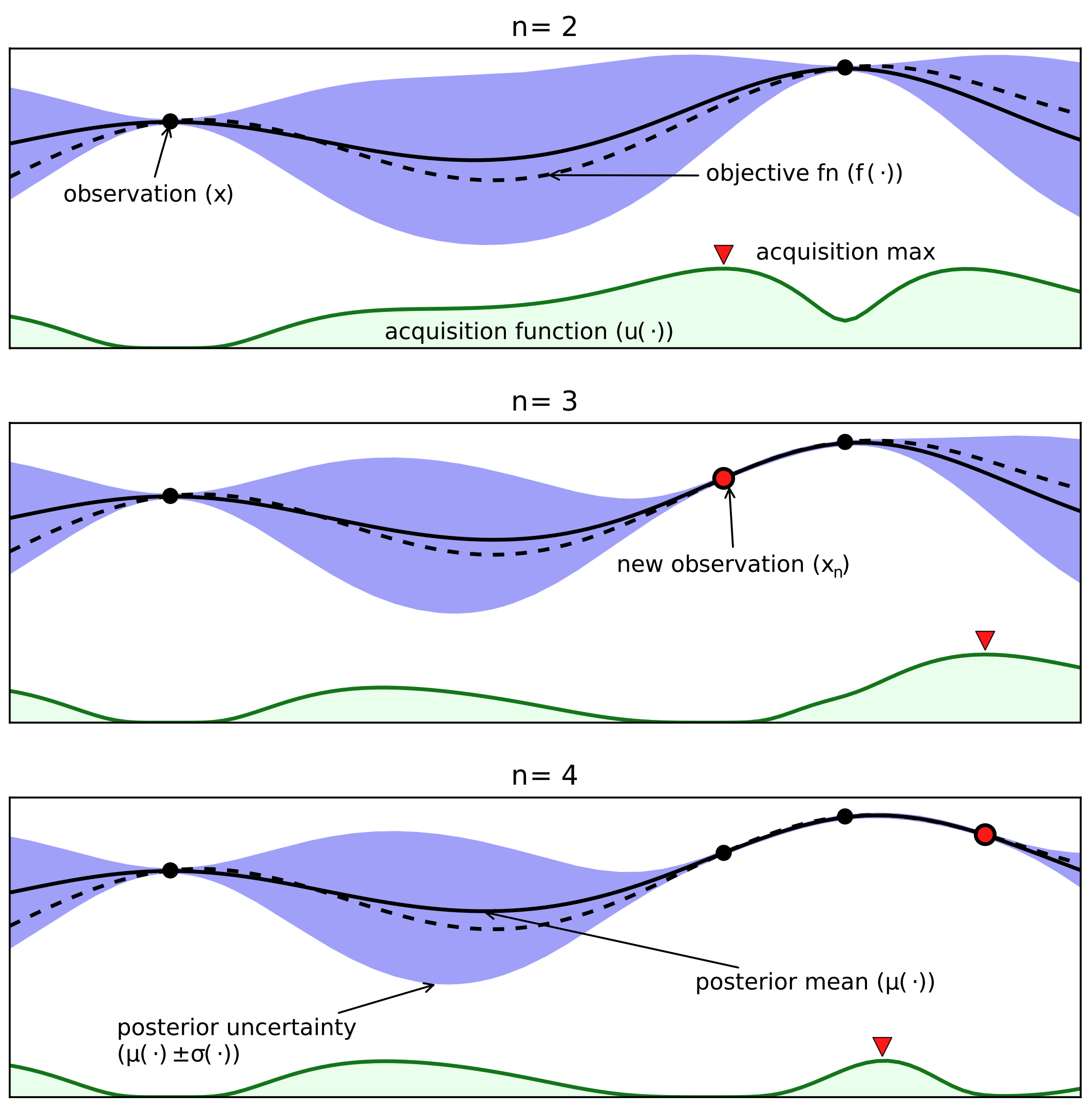
Figure 2: Bayesian Optimisation Visualisation from [30]

Three iterations of Bayesian Optimisation (iterations 2-4), with the dashed line representing the objective function and the solid line representing the probabilistic surrogate model.

3 Forecasting Ensemble

In forecasting, an ensemble can be used to combine a variety of different data sources and algorithm types to provide a more accurate and robust forecast. This chapter will provide a brief introduction to ensemble strategies, in particular those used in forecasting. It will further detail the ensemble method used for the general purpose forecasting setup at the core of this paper.
In general, the goal of ensemble learning is to use a combination of different algorithms and data augmentation to obtain multiple diverse models. These are then combined through aggregation, averaging or voting strategies, with the goal of getting a more robust and accurate prediction [34]. In the forecasting space, ensemble learning first originated in weather forecasting [35], where it has led to improvements in both accuracy and robustness of forecasts. Recently, ensemble forecasting has seen an increase in attention, with the top performing models in the M4 Competition [7] being ensembles.
When considering a set of forecasting algorithms all trained on the same data, one strategy for generating a good forecast of the resulting models is to simply use the model that performs best on the test data. Even though this approach may be intuitive and simple, it is naive in that it could make the resulting forecast overconfident if the test time series is not representative of the future. A more robust strategy could be to calculate an average over predicted values for each time step and use the resulting time series as the final prediction. To avoid having poorly performing algorithms decrease the ensemble performance, one can furthermore extend this strategy by only considering the $k$ best algorithms in the average. This can be done both on a global and a local level. In the former case, one would consider the performance across all items for selecting the $k$ best algorithms and would then use them to make inference for all of the items (time series). In the latter (local) case, one would evaluate the performance of all algorithms for each item individually and then select the $k$ best ones at an algorithm level. This can lead to different algorithms being selected for different items in the same dataset.
The forecast ensemble setup used in this paper uses a combination of local and global strategies to compute the ensemble. This leads to a three dimensional method, with a local, a global and a combination parameter. The local parameter is used to set a threshold for how well an algorithm needs to perform compared to the best performing one, on the item level, to be considered in the local ensemble. The global parameter follows the same concept but is used to compare models across all items. The combination parameter, is then used to set a threshold on a per item basis, for which strategy to use: global or local. The idea of this ensemble family (set of ensemble strategies parameterised by local, global and combination parameter) is to find a good trade of between the advantage of the local strategy, namely item level specificity and the robustness of the global strategy. Finding optimal values for these three parameters, respectively, finding a concrete ensemble strategy, is framed as another optimisation problem on a second test window. Since the precise mechanics of the ensemble family used are not subject of the empirical investigation of this paper, I will not delve into more detail here and further assume the strategy as a given.

4 Datasets

To ensure rigorous and verifiable results, all experiments included in this paper were conducted on a list of public open source datasets. This list includes the following four datasets: Covid Death [9], Solar [10], Electricity [11] and Kaggle retail [12]. These data sets were chosen due to their diverse characteristics, in terms of number of observations, number of items and frequency, and common use in the forecasting literature.

Covid Death: This is a dataset provided by the Center for Systems Science and Engineering at Johns Hopkins University [9]. The dataset is made up of 230 items (time series) with 212 time steps each. It was also used for benchmarks in [8][9] and contains reported coronavirus disease 2019 deaths on a daily basis, as visualized in Figure 3. The data is at the province level in China; at the city level in the USA, Australia, and Canada; and at the country level, otherwise. In the experiments, 30 days were forecasted for items in this dataset.

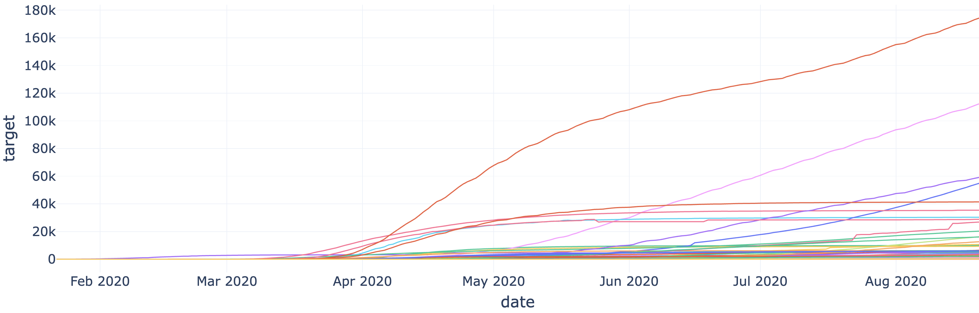
Figure 3: Covid death dataset overview

Solar: The Solar dataset [10], provided by the National Renewable Energy Laboratory of the U.S. Department of Energy, provides data on the energy production of photovoltaic power stations on an hourly basis, as visualized in Figure 4. It contains 137 items, with 7033 time steps each. In the experiments, 168 hours (7 days) were forecasted for items in this dataset.

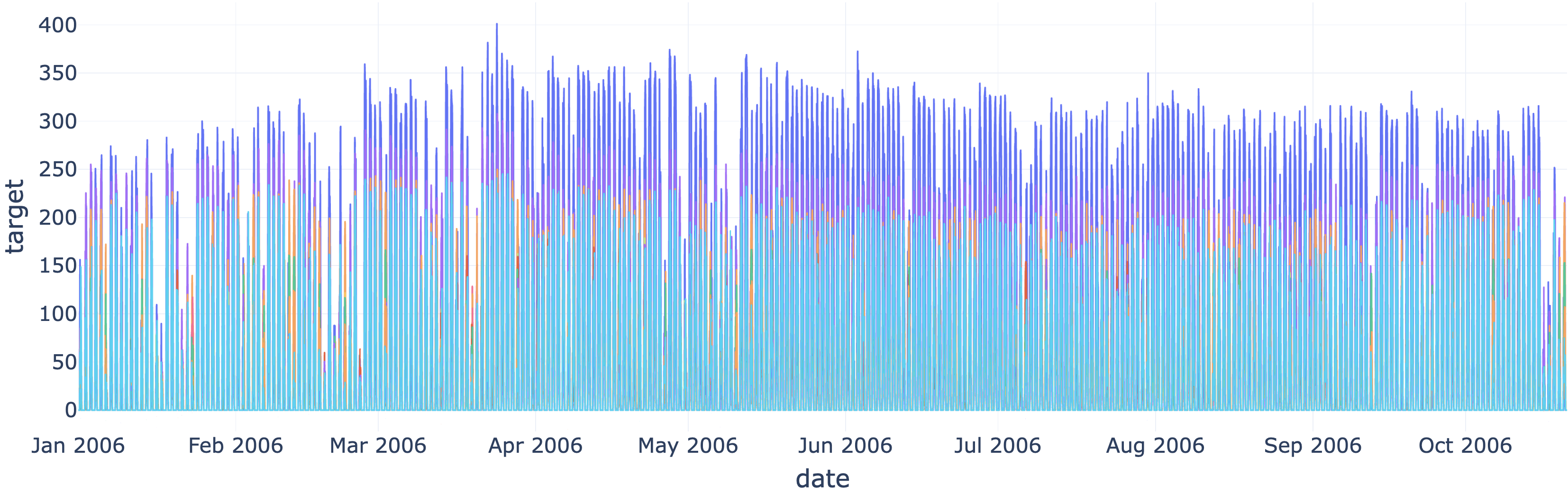
Figure 4: Solar dataset overview

Electricity: This dataset [11], as also referenced by [2][36][37], contains energy consumption of 370 different clients (370 items) with 4032 observations each in hourly frequency, with no missing values, as visualized in Figure 5. In the experiments, 168 hours (7 days) were forecasted for items in this dataset.

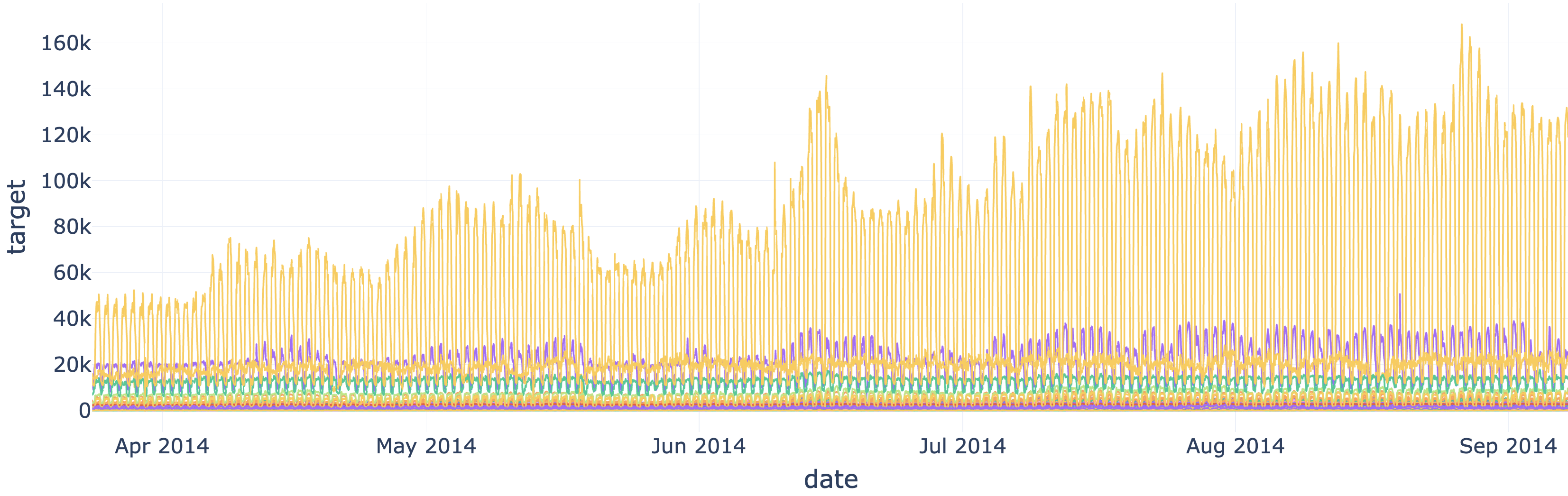
Figure 5: Electricity dataset overview

Kaggle retail: The Kaggle retail dataset [12], as used in the experiments, contains data on the number of sales of different product families at a daily frequency, as visualized in Figure 6. It includes 54 different items with 1684 time steps each and is used with a forecasting horizon of 14 days in the experiments.

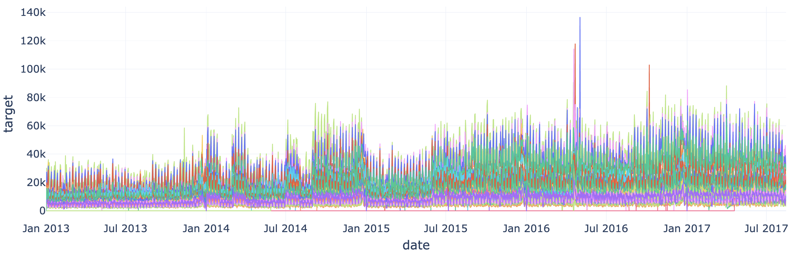
Figure 6: Kaggle retail dataset overview

5 Experiments

This chapter contains the design and evaluation of results for all experiments conducted as part of this paper. Due to the relatively low number of repetitions for each experiment with different random seeds, the use of p-values may be misleading and is therefore avoided throughout the chapter. It instead uses mean values and standard deviations for the comparison of results.

5.1 Impact on Individual Algorithms

The scientific question of this paper is based on the premise that HPO provides accuracy improvements to single algorithms. This makes it then further reasonable to explore how this improvement affects the accuracy of a forecasting ensemble. In the following, this paper shows that the aforementioned premise is true for the deep learning algorithms in question. To be precise, this section explores the setup and results of experiments which quantify the accuracy and cost changes from adding HPO to individual algorithms, namely DeepAR and MQ-CNN. The setup compares the results of two different machine learning pipelines: pipeline_1 and pipeline_2. In machine learning, a pipeline is used to automate workflows, including data preprocessing and transformation as well as model training and inference.

In this case, the first pipeline is setup to do data processing, converting the data into long format and splitting it into training and testing partitions, it then trains a single model on the train set $\mathbf{z}_{1:t-k}$, with $t$ being the total number of observations and $k$ being the length of the forecasting horizon. Finally, the pipeline does a single backtest to calculate the relevant performance metrics. Backtesting refers to the concept of evaluating the performance of a forecasting model based on historical data. Here the model trained on $\mathbf{z}_{1:t-k}$ does inference for $t-k+1:t$ and is then evaluated on the test set $z_{t-k+1:t}$.
The second pipeline is structured similarly in that it does data processing in the same way, leading to an identical data foundation. However, with different data partitions. This is because pipeline_2 was not setup to train a single model, but instead to train multiple models using HPO on a train set $\mathbf{z}_{1:t-2k}$. The HPO strategy then does backtests for each trained model on the test set $\mathbf{z}_{t-2k+1:t-k}$ to determine the best performing one. The resulting, winning hyperparameter configuration is used to train a single model on $\mathbf{z}_{1:t-k}$, which is evaluated on the validation set $z_{t-k+1:t}$, making it comparable to the model resulting from pipeline_1.

The HPO strategy used in this set of experiments is Bayesian Optimisation as described in subsection 2.3. It was not chosen based on any empirical data, which follows in subsection 5.2 on the ensemble experiments, but rather due to it being one of the most popular HPO strategies, as suggested by [38]. This is valid, since the premise of this section is not to provide an optimal strategy, but to show that HPO does add a performance improvement to the selected individual algorithm, for which, any HPO technique that shows this, suffices. In the tuning workflow of pipeline_2, Bayesian Optimisation is run with 15 total iterations (max_training_jobs $=15$), 5 of which are running in parallel at a time (max_parallel_jobs $=5$), leading to only 3 sequential steps. This configuration was not chosen based on empirical evaluations, but rather on internal experience and intuitive heuristics. However, an in depth analysis of optimal configurations is part of subsection 5.2.
The hyperparameters that are tuned vary by model. ForDeepAR, HPO tunes the learning rate as a continuous hyperparameter parameter and context length as a discrete (integer) parameter. The hyperparameter tuned for MQ-CNN is context length. The range of context length is dynamically set based on the given forecast horizon of the time series data used.
To ensure robustness, pipeline_1 and pipeline_2 were tested on both DeepAR and MQ-CNN. Each algorithm was run on all datasets (covid_death, solar, electricity and kaggle_retail). The metrics MAPE, MASE, WAPE, wQL-90, wQL-50, wQL-10 and avg-wQL were computed for each of the resulting $2*2*4=16$ experiments. To simplify the following comparison, the experiments are only compared based on their avg-wQL. This choice is based on the fact that every metric used except MASE correlates above 0.98 with the avg-wQL, using the standard pearson correlation coefficient, making it a a representative selection, as detailed in B.
The comparison is further simplified by computing the mean avg-wQL across all datasets for both MQ-CNN and DeepAR. This leads to a direct comparison between accuracy with and without HPO for each algorithm as shown in Figure 7. The raw results from the experiments can be found in appendix Appendix A.

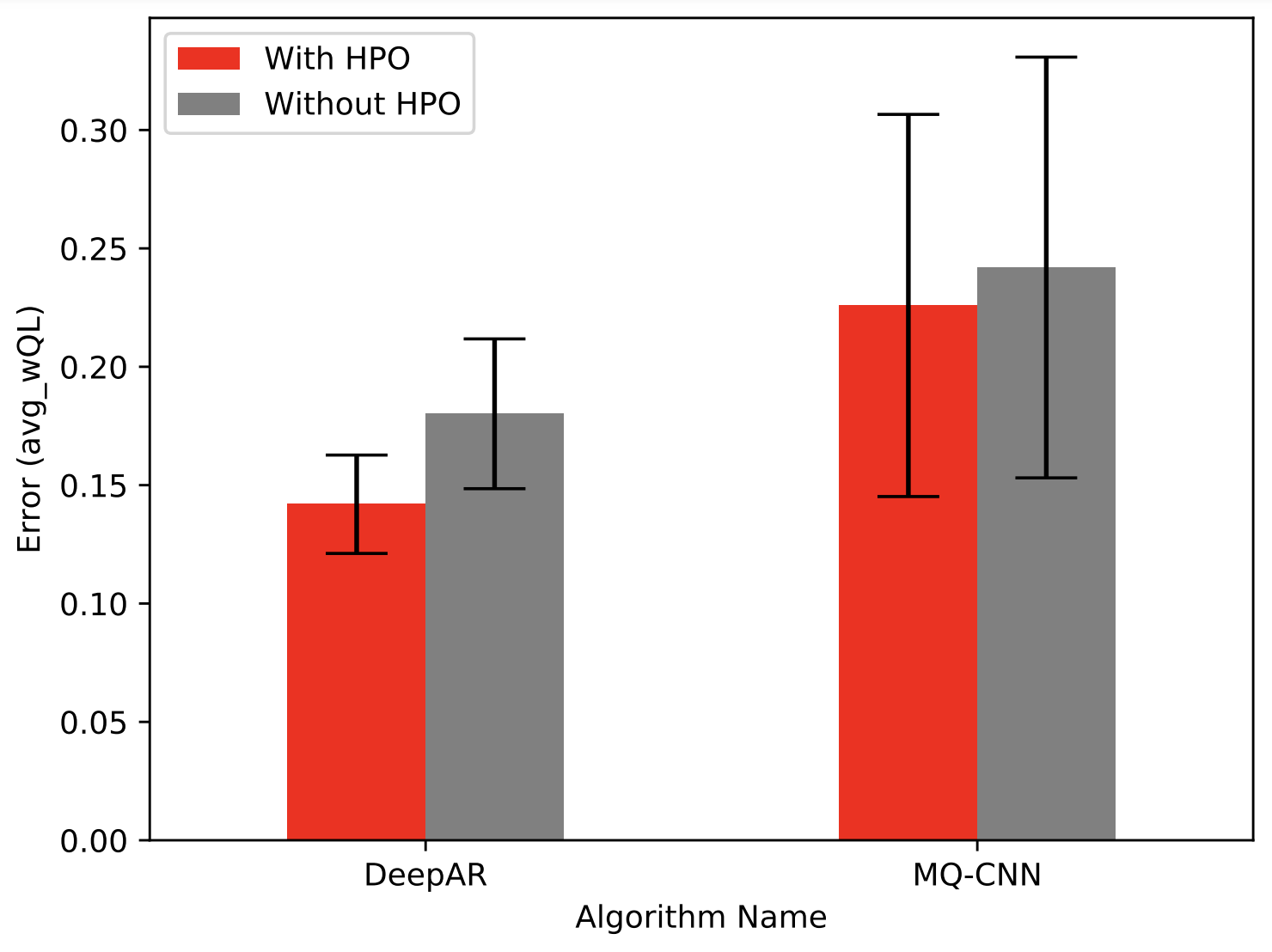
Figure 7: Individual Algorithm Accuracy With and Without HPO

With 4 observations per experiment, a mean model accuracy with HPO of 0.1419 (variance of 0.0208) and a mean accuracy without HPO of 0.1801 (variance of 0.0316), adding HPO reduces the mean avg-wQL for DeepAR by 21.2 %. For the experiments with and without HPO based on MQ-CNN, adding HPO leads to a reduction in error (avg-wQL) of 6.6 %.
These experiments show that HPO improves the accuracy for both DeepAR and MQ-CNN. This shall serve as indication evidence that HPO can have a positive impact on algorithm performance, and therefore may also improve the performance of a AutoML forecast ensemble as further discussed in subsection 5.2.

Next to the impact of HPO on model accuracy, the second interesting aspect is that of training latency. Intuitively the additional models trained as part of hyperparameter tuning are expected to affect the latency and training cost. Even though most literature in the machine learning community only considers accuracy, latency may greatly affect the busyness aspect of an AutoML forecasting platform similar to the one described in subsection 5.2.
Hence, it makes sense to also consider latency and cost effects of added HPO. The former refers to the duration of a workflow (pipeline) or sub-workflow such as the training of a single model (wall time) and the latter refers to the amount of compute resources consumed as part of a workflow (pipeline) or sub-workflow (instance run time). The two may not always correlate due to the varying amount of parallelization utilised in HPO. For example, when running two workflows, both using random search, one with max_training_jobs $=15$ and max_parallel_jobs $=1$ and the second with max_training_jobs $=15$ and max_parallel_jobs $=15$. They will both have the same HPO cost since the number of models trained is 15 in both cases, leading to an identical consumption of resources for HPO. The HPO latency, however, will differ between the two runs. For the first one with max_parallel_jobs $=1$, all models are trained sequentially, leading to the latency being computed as the sum of all individual model training latency. The tuning job with max_parallel_jobs $=15$ will train all models in parallel, leading to the overall latency being computed as the latency of the model with the longest training duration. Assuming all models train for the same duration, this leads to the former being 15 times slower in terms of latency than the latter.
Since the experiments outlined in this section all use the same degree of parallelization, latency and training cost can be used interchangeably for comparisons. For better interpretability, the following comparison will be made using latency in seconds.

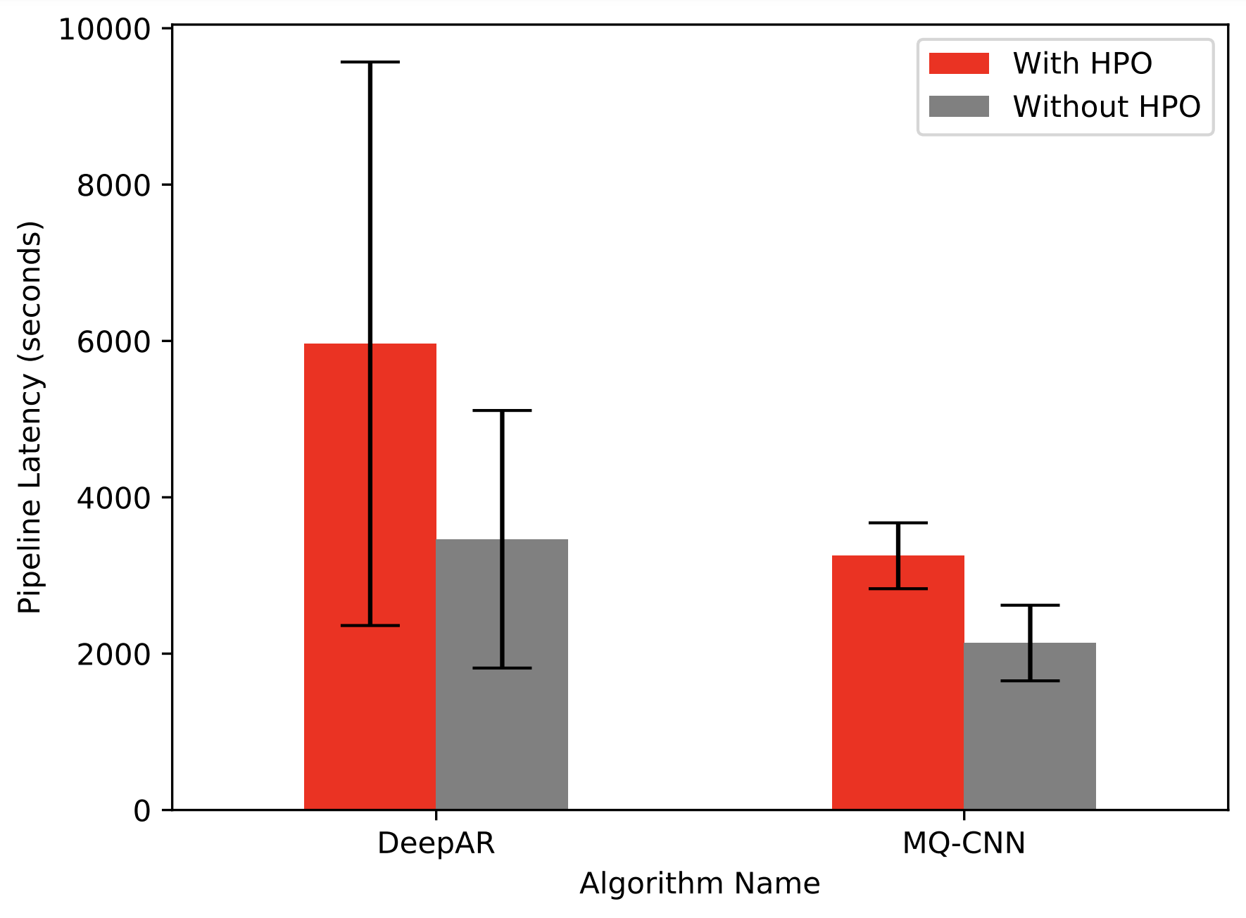
Figure 8: Individual Algorithm Latency With and Without HPO

The values plotted in Figure 8 are mean end-to-end pipeline latency with and without HPO for both DeepAR and MQ-CNN. The error bars indicate the standard deviation of latency across datasets. One can recognize the following trends in the plot: Firstly, DeepAR is on average 72 % slower than MQ-CNN (with HPO it is 83.4 % slower and without HPO it is 62.1 % slower). Secondly, HPO adds an increase of 52.3 % to the end-to-end pipeline latency, for MQ-CNN, whereas the increase in latency for DeepAR when adding HPO is 72.2 %, resulting in an average increase of 62.2 %. This shows that the accuracy improvement of HPO is accompanied by a considerable increase in training latency, indicating the necessity for a trade-off between the two. This is further discussed in following sections.

5.2 Forecast Ensemble

This section addresses the core scientific question of this paper by delving into the cost and accuracy effects of various HPO strategies on the performance of a general AutoML forecast ensemble. In particular, this section contains an evaluation of experiments comparing the effect of adding HPO to DeepAR and MQ-CNN on the performance (accuracy and latency) of an ensemble containing ARIMA, ETS, NPTS, Prophet, MQ-CNN and DeepAR. This paper compares different HPO strategies, namely Bayesian and Hyperband (subsection 5.5) and different variations of these strategies, namely various different numbers of max_training_jobs. This parameter refers to the maximum number of models trained as part of HPO before the best configuration is determined. The parameter max_parallel_jobs refers to the number of models that are trained in parallel as part of hyperparameter tuning. It was not extensively explored and is therefore not the subject of further discussions. In the following experiments max_parallel_jobs kept at a constant rate of 5.

Similarly to the individual algorithm experiments outlined in subsection 5.1, the forecast ensemble setup was implemented as an end-to-end machine learning pipeline. It consists of 4 steps: (1) data preparation, (2) hyperparameter tuning, (3) ensemble selection (4) final model training. Data preparation and processing are identical to that of pipeline_2 in subsection 5.1, leading to a training dataset $\mathbf{z}_{1:t-2k}$, a test dataset $\mathbf{z}_{t-2k+1:t-k}$ and a validation dataset $\mathbf{z}_{t-k+1:t}$, which are disjoined.
The second step of the pipeline, hyperparameter tuning and model training, is executed in parallel for each algorithm. In the case of the non-deep-learning-based algorithms, that is ARIMA, ETS, NPTS and Prophet, model training is conducted on the training partition using default hyperparameters that have been empirically shown to perform well across datasets, leading to one trained model for each. Depending on the parametrisation of the pipeline, HPO may be performed for the deep-learning-based models. If hyperparameters are not to be tuned using HPO, then this step follows the same procedure for both DeepAR and MQ-CNN as for the non-deep-learning-based models. If hyperparameters are to be tuned, the step has the following outline: First, the training dataset $\mathbf{z}_{1:t-2k}$ with length $l$ is further split into a training partition for tuning $\mathbf{z}_{1:l-k}$ and a validation partition for tuning $\mathbf{z}_{l-k+1:l}$. Using a given Hyperparameter tuning strategy, max_training_jobs models are trained on the training partition for tuning and evaluated on the validation partition for tuning. The best performing algorithm configuration is then used to train a final model on the entire training dataset $\mathbf{z}_{1:t-2k}$. This results in one model being trained for each algorithm.
In the next step, the ensemble of these algorithms is generated (as outlined in section 3). Ensemble selection uses the models trained on $\mathbf{z}_{1:t-2k}$ to make inference on $t-2k+1:t-k$. These predictions, together with the true values in the test partition $\mathbf{z}_{t-2k+1:t-k}$ are then used to parameterise the ensemble family, resulting in the concrete configuration of the ensemble strategy used for forecasting.
The parameters of the ensemble strategy are determined by HPO, in particular using the global optimization strategy Basin-Hopping [39]. With the resulting ensembles being evaluated on the validation set $\mathbf{z}_{t-k+1:t}$. The winning ensemble parameters (local, global and combination parameters) are then used to determine the concrete ensemble to be used based on another set of models (one for each algorithm) trained on training and test sets $\mathbf{z}_{1:t-k}$ and evaluated on validation. This means, that in this last step, we choose a specific combination of models for each item, resulting in the final ensemble. This ensemble is then evaluated on the validation partition to compute the metrics also used for all the following comparisons in this chapter. The risk of overconfident predictions which is associated with this way of evaluating the ensemble, is recognised, but was not accounted for due to time constraints.

The previous steps lead to the forecast ensemble pipeline having the following parameters and input variables: the dataset used for training, a binary which determines if hyperparameters are to be tuned or if default ones should be used, and in the former case, additional parameters for the maximum number of models trained by HPO, the maximum number of models trained in parallel and the HPO strategy. After initial exploration, all other parameters where regarded as static, logically set, or are learned by the pipeline and shall not be a further subject of this paper.

All experiments, testing a particular configuration of pipeline parameters were repeated with three different random seeds for each of the four datasets, yielding a total of 12 runs per experiment, to ensure more rigorous results.

5.3 Impact of Default HPO on the Ensemble

Before delving into the empirical evaluation of different HPO strategies and their configurations in the following subsections, this one will look at a comparison between the effects of HPO on individual algorithms as outlined in subsection 5.1 and its effects on the final forecast ensemble.
To make the magnitude of the effect on the ensemble comparable to the effect on individual algorithms, this subsection is going to look at experiments conducted with the HPO strategy being Bayesian, the number of models trained for tuning max_training_jobs $=15$ and max_parallel_jobs $=5$, as was done in the experiment including individual algorithms outlined in subsection 5.1. When considering the effect of adding HPO to DeepAR and MQ-CNN in the ensemble, as shown in 9(b), it is apparent that differences are more marginal compared to those observed for the individual algorithms.

Figure 9: Ensemble Performance With and Without HPO

(a) Accuracy

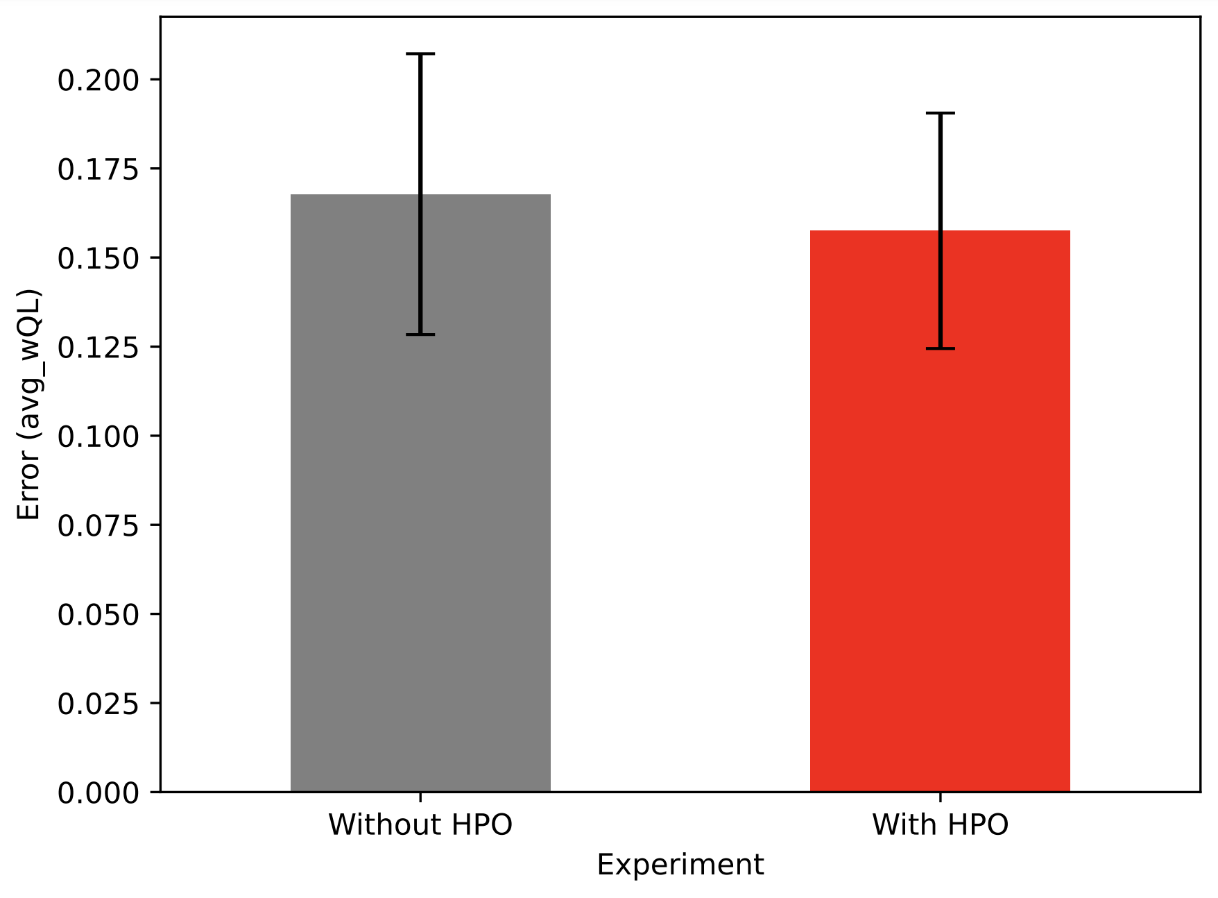
(b) Pipeline Latency

This is both true for the difference in error, with HPO leading to a 6.1 % decrease, visible in 9(a) and the difference in end-to-end pipeline latency, with a 14.0 % increase caused by adding HPO. The former can be partly explained by the added improvement of other algorithms included in the ensemble (ARIMA, ETS, NPTS, Prophet). For example, if results from these other algorithms improve the forecast, then this diminishes the positive accuracy effect on the final forecast of adding HPO to DeepAR and MQ-CNN. The latter difference can be explained by overall higher latency of the pipeline compared to the one used for the individual algorithms, caused by extra steps such as ensembling. These extra steps increase the overall pipeline latency and therefore reduce the relative increase in latency caused by HPO.
The differences in effect size of adding HPO to the deep-learning-based algorithms is visualized in Figure 10, which compares the resulting accuracy change for individual algorithms as well as the ensemble.

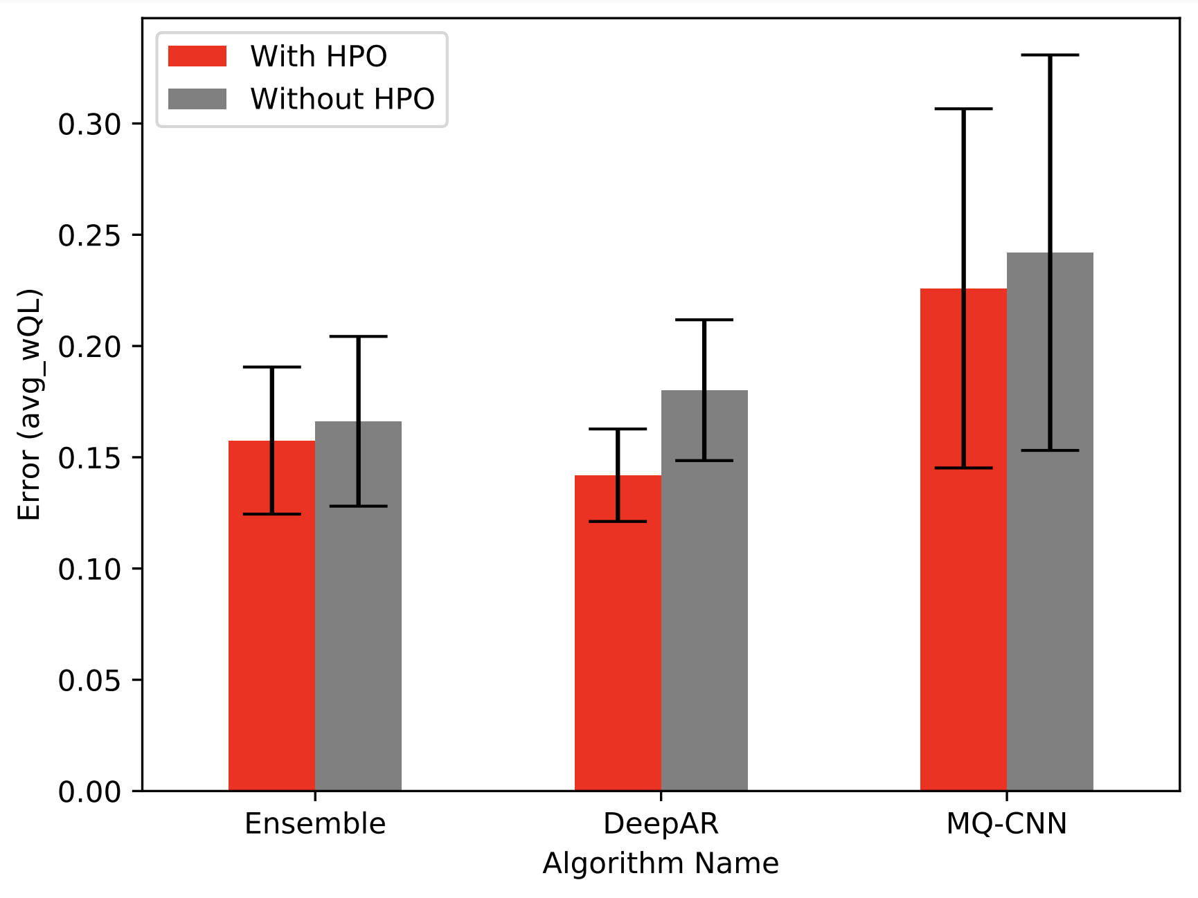
Figure 10: Individual Algorithm vs. Ensemble

This comparison shows that the ensemble pipeline without HPO leads to 19.5 % more accurate results on average, than both DeepAR (8.4 % higher error) and MQ-CNN (45.6 % higher error) individually without HPO (grey bars), demonstrating the positive effect of ensemble learning on forecast accuracy. When comparing the effect size of adding HPO to the individual algorithms and the ensemble, it is noticeable that this effect is smaller for the ensemble due to the aforementioned reasons. To be precise, for DeepAR, HPO improves accuracy by 21.2 % and for MQ-CNN 6.6 %, leading to an average improvement for the individual deep-learning based algorithms of 13.9 %. Whereas the accuracy improvement of adding HPO to the deep-learning algorithms on the final ensemble is only 5.2 % using Bayesian Optimisation with 15 models trained for tuning, five of which in parallel. It is further noteworthy that DeepAR with HPO has the overall lowest accuracy in this comparison. The reason for this is not clear. However, it would make sense to assume that the trade-off between rigorous results and high test performance in ensemble strategy selection, could be the cause.
These results indicate that using the ensemble pipeline provides better results than the individual algorithms without HPO and further that adding HPO to the ensemble pipeline can further improve its performance.

5.4 Experiment Configuration Overview

To show that the positive impact on the ensemble performance of adding HPO to the deep-learning-based algorithms can be further increased, other optimisation strategies as well as configurations of those where tested. The following subsection provides an overview of the conducted experiments. This includes experiments with Bayesian Optimisation and Hyperband as well as permutation of these strategies with different numbers of max_training_jobs. As mentioned before, each concrete configuration is repeated 12 times (on 4 different datasets, with 3 different random seeds each).
An overview of all experiments conducted can be seen in Figure 11, with the x-axis being the mean latency HPO of a given configuration and the y-axis being the mean avg-wQL. This figure is to be read such that one is ideally looking for a configuration on the bottom left with low latency and low avg-wQL. Throughout this paper, configurations without HPO are grey, those with Hyperband are orange and the Bayesian Optimisation ones red. Note that the figure is not comparing the overall pipeline latency here, but rather the latency of hyperparameter tuning, since the latency of components other than HPO is assumed to stay relatively constant.
The evaluation of results is detailed in the following sections. Looking only at HPO makes the effects of different configurations more pronounced and therefore easier to evaluate. To make the direct comparison of different numbers of max_training_jobs easier, the number of max_parallel_jobs is kept at a constant of 5. A table with the results of all experiments can be found in Appendix C.

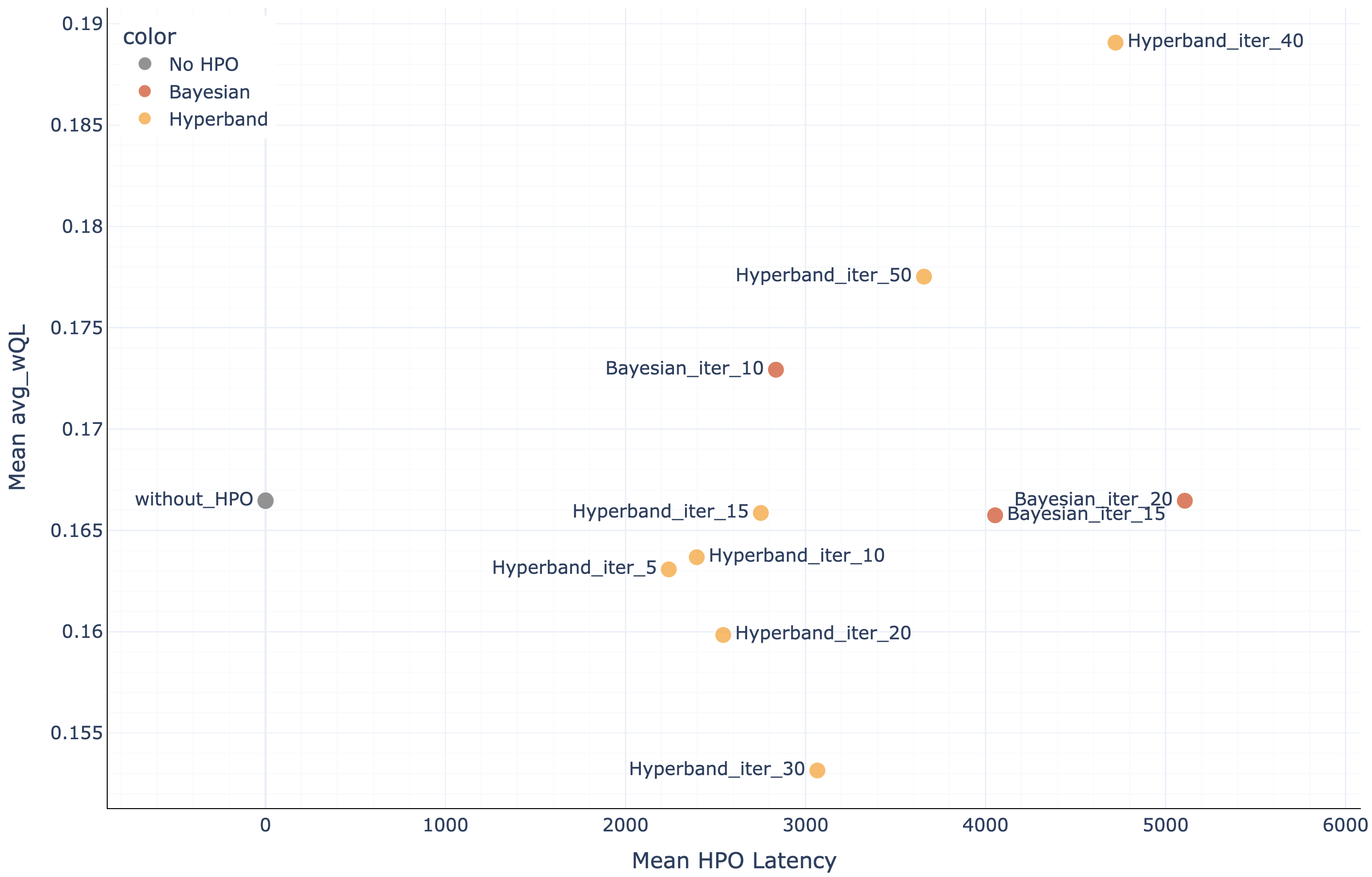
Figure 11: Experiment Overview

As the experiments are mainly differentiated by two characteristics, namely tuning strategy and number of training jobs max_training_jobs, it makes sense to analyse the results along these two dimensions. This is advantageous as it breaks the problem of determining an optimal configuration down into two simpler problems: (1) find an optimal strategy and (2) find an optimal setting of max_training_jobs for that strategy. In an ideal case, optimal refers to a strategy that is both faster and more accurate than any other reasonable configuration. Such an optimum could not be found as part of this paper and is unlikely to exist because model accuracy positively depends on training time for low latencies (ambivalent for higher latencies as they may increase model variance). This paper instead aims at finding a reasonable trade-off between accuracy and latency, as defined in subsection 5.6. A comparison between Hyperband and Bayesian optimisation is conducted in the following subsection 5.5 and an extension of this comparison, by varying the number of max_training_jobs, is described in subsection 5.6.

5.5 Hyperband vs. Bayesian Optimisation

This subsection compares the performance of the ensemble pipeline with HPO, either using Hyperband or Bayesian Optimisation as a tuning strategy. There are several approaches in which one can execute this comparison, such as comparing a single sample configuration, as was done in the individual algorithm evaluation in subsection 5.1 and in subsection 5.3 on the impact of default HPO on the ensemble. This approach may have been valid there, as these comparisons have the sole purpose of showing that an effect exists for which any configuration that does this suffices. This section, however, aims at answering the question of a generally better strategy in the context of the AutoML forecast ensemble, requiring a more representative approach. This is achieved by comparing the two strategies for multiple configurations respectively.

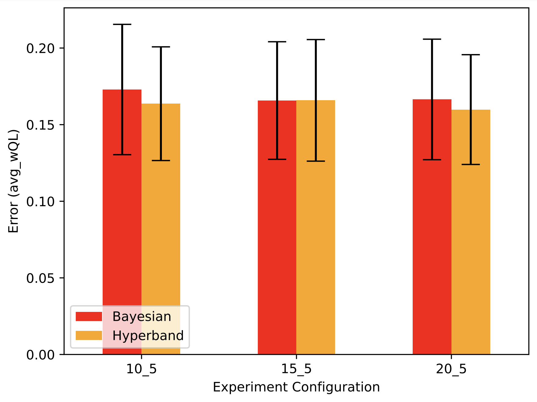
Figure 12: Experiment Overview Accuracy

The error comparison of the final ensemble with the two strategies couldn’t show that there is a substantial difference between Hyperband and Bayesian Optimization. This was determined by comparing both strategies for 3 different configurations of max_training_jobs and max_parallel_jobs. To be precise, Hyperband 10;5 is compared to Bayesian 10;5, Hyperband 15;5 is compared to Bayesian 15;5 and Hyperband 20;5 is compared to Bayesian 20;5, with the first number always referring to the number of max_training_jobs and the second number denoting the number of max_parallel_jobs. This comparison is shown in Figure 12.

The difference between Hyperband and Bayesian is minor for all variations of max_training_jobs and max_parallel_jobs tested (10;5, 15;5 and 20;5). This does not mean that HPO with Bayesian Optimisation has the same effect on the accuracy of the individually tuned algorithms as HPO with Hyperband, but rather indicates that no large effect on the accuracy of the final ensemble can be detected. This may be due to the relatively small number of 4 repetitions with different random seeds for each experiment. Hence, no optimization strategy can be regarded as much better based on its accuracy. One could, however, interpret the fact that the mean error of Hyperband is on average 3.1 % lower than that resulting from Bayesian Optimisation, as an indicator that the former may be better.

When comparing the ensemble performance based on latency, Hyperband outperforms Bayesian Optimisation. The design of the latency comparison is structured the same as the accuracy comparison, with, Bayesian max_training_jobs_i; max_parallel_jobs_i being compared to Hyperband max_training_jobs_i; max_parallel_jobs_i as shown in Figure 13.

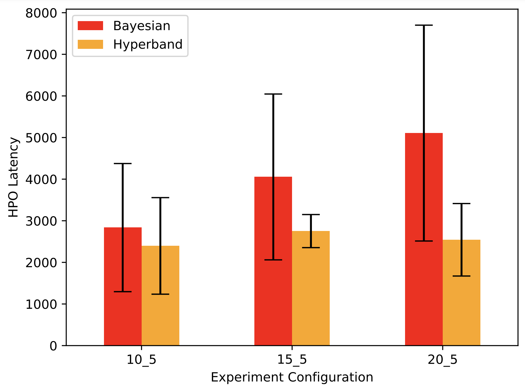
Figure 13: Experiment Overview Latency

The comparison shows that for Hyperband, the mean latency of Hyperband is consistently lower than that of Bayesian Optimisation. It is further noticeable that Hyperband latency doesn’t increase much with higher numbers of models trained for tuning. For 15 trained models, the HPO latency of Hyperband is only 14.9 % higher than the latency for 10 models. Going from 15 to 20, the latency even decreases again by 7.6 % (which is expected to be due to random variation and not to be an effect of the increased number of models), overall, leading to a standard deviation between latencies of different configurations of 146.1 seconds, whereas the standard deviation latencies for Bayesian optimisation is higher with 928.0 seconds. Here we see a clear increase in latency with higher numbers of trained models for tuning (42.9 % from 10 to 15 trained models and another 26.0 % from 15 to 20 trained models). This makes Hyperband favorable over Bayesian optimisation in terms of latency as it is on average 32.6 % faster.
Overall, this makes Hyperband more suitable for use in the AutoML forecast ensemble, indicating both slightly better accuracy results as well as a lower latency. This is the reason why the focus of further experiments that are part of subsection 5.6 is on Hyperband.

5.6 Tuning Strategy Variations

This section will explore AutoML forecast ensemble pipeline results with different variations of resource allocations for HPO, focusing on the Hyperband optimisation strategy. As suggested by [40], Hyperband can be parallelized in a way that doesn’t change training cost but reduces latency (if max_training_jobs remains constant at 5 and only max_parallel_jobs is increased). Such variations of max_parallel_jobs are not assumed to affect the accuracy of the final ensemble. Therefore, this analysis will only consider the total number of jobs, for the sake of simplicity. Trade-offs between latency and cost (meaning max_training_jobs and max_parallel_jobs) can be arbitrarily chosen for particular usecases.

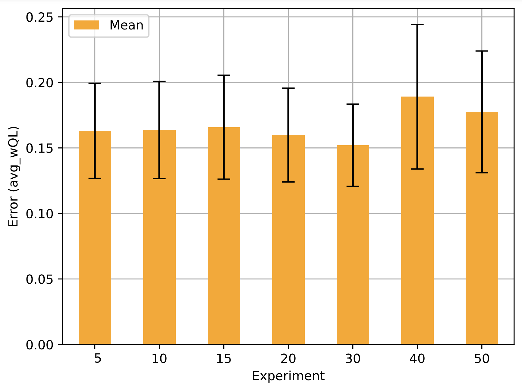
Figure 14: Hyperband Metric Overview

The variations in accuracy resulting from different numbers of max_training_jobs, are shown in Figure 14. These differences are measured as differences in the mean of the distributions of all experiments performed with a particular configuration (in the plot this distribution is indicated by its mean and standard deviation). The bars are each labeled with two numbers separated by an underscore. The x-axis refers to the number max_training_jobs. The number of max_parallel_jobs is kept at a constant rate of 5.

In the above plot one can see that for max_training_jobs $\in\{5,10,15\}$ the avg-wQL stays relatively constant. For a higher number of iterations, e.g. max_training_jobs $\in\{20,30\}$, it then decreases, improving model performance, until then increasing again for max_training_jobs $\in\{40,50\}$, potentially due to hyperparameter over-fitting. Meaning that the hyperparameters selected perform very well during training, but don’t generalize well to the validation partition for tuning, leading to a higher error. The configuration with the lowest mean error across all experiments and repetitions is that with 30 trained models. It is 4.9 % better than the second best configuration with 20 models trained for tuning and 19.6 % better than the worst configuration test with 40 models trained.

When considering the latency differences of the Hyperband configurations, one can observe an increase with higher numbers of trained models. This behaviour is expected, as with a constant number of max_parallel_jobs an increased number of max_training_jobs leads to more sequential training jobs, which increases latency. This trend is not monotonic, which could be partly attributed to the randomness in the dynamic early stopping behaviour of Hyperband. An example of this would be that a tuning job which is supposed to try 20 different configurations, stops 15 of them very early, because they are not promising. A tuning job with 10 configurations may only terminate 5 early, because they are not promising. This leaves both variations with 5 models left to train, minimizing the latency difference between them, or possibly even reverting it.
Figure 15(a) shows the mean latency across datasets for different numbers of models trained per tuning job, with the error bars indicating the standard deviation (of the different means across runs for each dataset, with variation within repetitions of a single dataset being disregarded). This loss of information is remedied in 15(b), which shows a more granular latency comparison at a per dataset level.

Figure 15: Hyperband Latency Overview

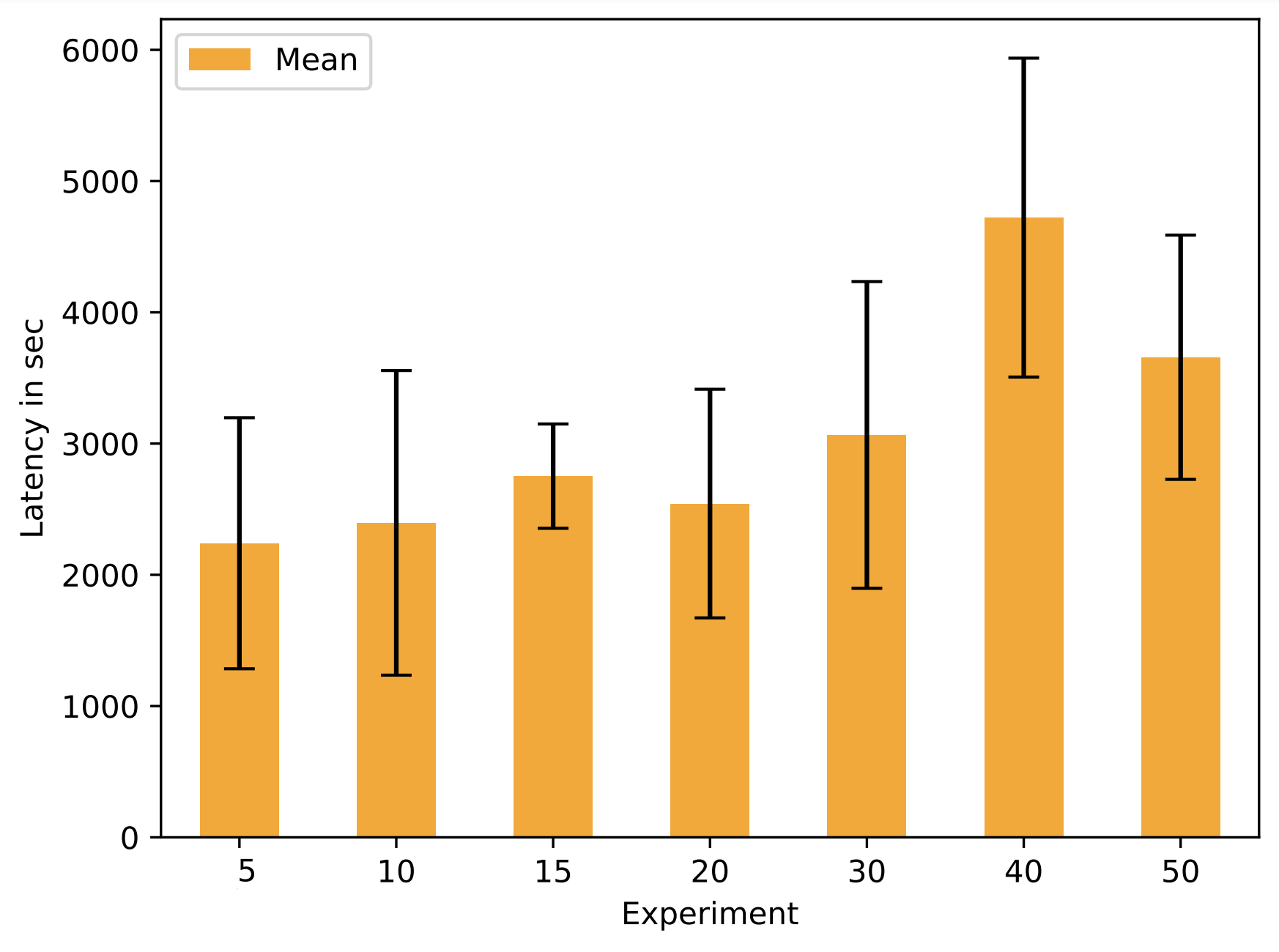
(a) Average Across Datasets

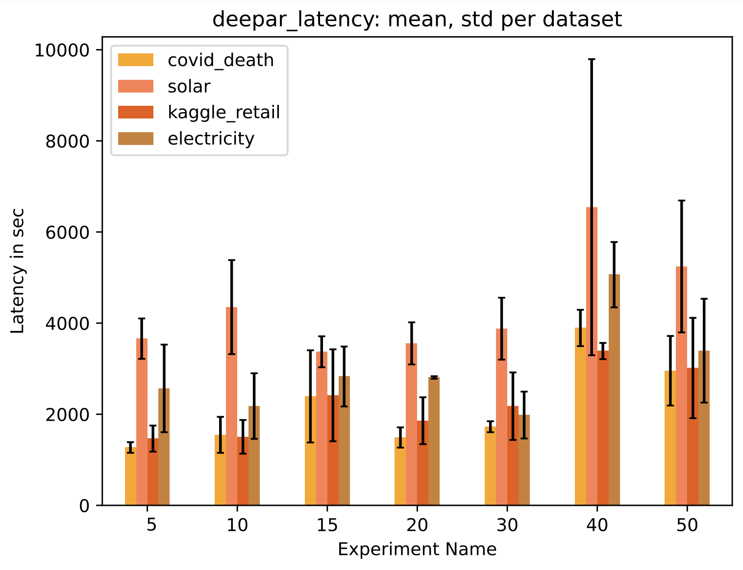
(b) Per Dataset Latency

The latency comparison on the dataset level, also reflects the qualities of the different datasets, namely number of items and number of time steps. The solar dataset monotonically has the highest mean latency for all of the evaluated configurations, which can be presumably attributed to it also having the highest number of time steps (that is, 7033). This hints at the fact that the number of time steps is more indicative of tuning (and therefore also training) latency than number of items, or number of data points ($n\_items*n\_time\_steps$), since solar is not first in either of those. This is supported by the fact that the electricity dataset, which has the highest number of data points (1491840, which is 54.8% more than the solar dataset with 963521) and the second highest number of time steps (4032), has the second highest latency for all configurations except one. This difference in tuning latency is not as pronounced for the smaller datasets, covid death (with 48760 time steps) and kaggle retail (with 90936 time steps), as these two are comparable in latency for most datasets, with one or the other being faster at times.

As can be expected, the smallest number of total models trained during tuning also has the smallest latency. As the optimal configuration in terms of latency (5;5) does not coincide with the optimal configuration for accuracy (30;5). This means a trade-off has to be made. This trade of can be conceptualised as a discrete linear optimisation problem Equation 17, where $latency(\cdot)$ and $error(\cdot)$ return the normalised latency and error respectively and $\theta_{0}\in[0,1]$ being a weight that determines how much latency and error should each affect the outcome.

$$\min(\theta_{0}*latency(conf_{i})+(1-\theta_{0})*error(conf_{i}))$$ (17)

These weights should be set depending on the business use case at hand. For example, if latency is not important at all, $\theta_{0}$ is set to $0$, leading to Hyperband with max_training_jobs $=30$. If one primarily cares about latency and error is only of secondary importance, then one can set $\theta_{0}=1$, leading to Hyperband with max_training_jobs $=5$ being optimal. It is important to note, that even though latency and error are normalized, $\theta$ is not necessarily a linear indicator. Meaning that a $\theta$ does not directly mean we equally care about latency and error, since a non-symmetric distribution in either may skew results.

An analysis of Equation 17 shows that for $\theta_{0}\leq 0.1798$ the configuration Hyperband with max_training_jobs being 30 is optimal, for $\theta_{0}>0.1798$ the configuration Hyperband with max_training_jobs being 5 is optimal. This relationship is visualized in Figure 16, which shows the value of Equation 17 for the continuous variable $theta$ (y-axis) and the discrete variable $conf_{i}\in\{5,10,15,20,30,40,50\}$ (x-axis), which indicates the max_training_jobs. The color associated with a given tuple of tuning configuration and theta shows the cost of Equation 17, with lighter colors indicating a lower cost (better configuration).

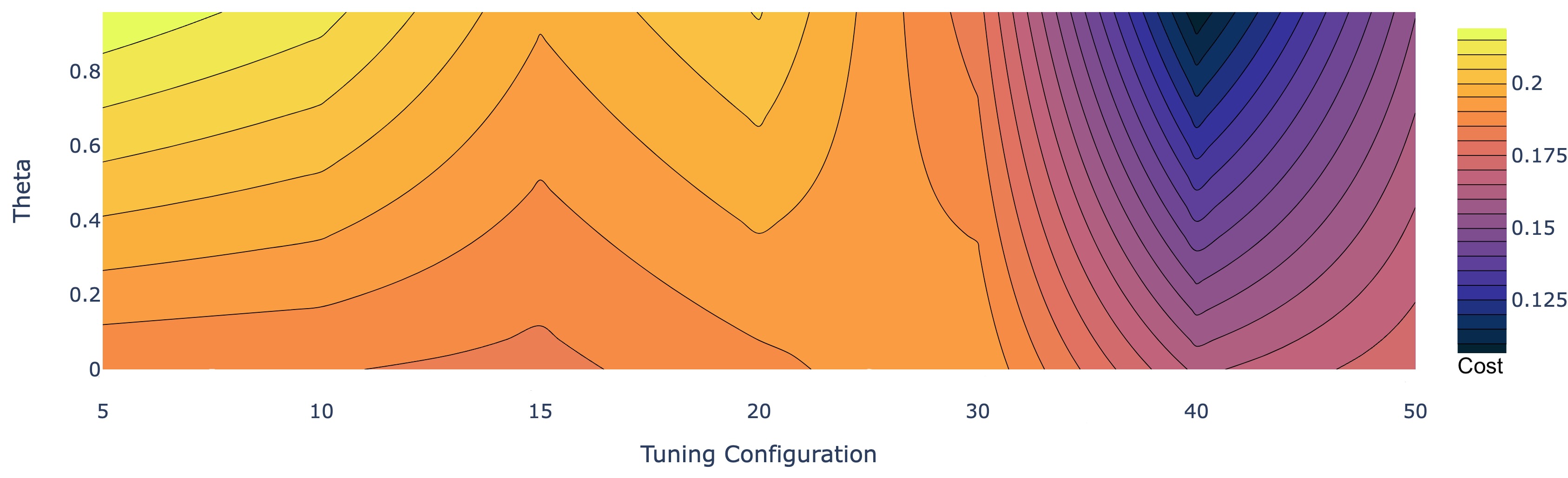
Figure 16: Accuracy vs. Latency Trade-Off

The figure is to be read horizontally with the optimal configuration being that where the cost is lowest (where the color is lightest). In the figure, the number of max_training_jobs $=30$ is best for all $\theta$ below $~{}2.8$. This is due to the low frequency of the contour lines, which was chosen to increase readability. With a higher frequency, one could better approximate the true cutoff point visually (this was not done because it makes it harder to differentiate the colors used and therefore also to read the figure). The plot instead has the purpose of roughly estimating a good configuration and to provide an intuitive understanding of the relationship between tuning configuration and theta. A table with the normalized accuracy and latency results as well as an overview of the convex combination of the two can be found in Appendix D.

The result of this evaluation of Hyperband is also reflected when comparing all experiments, visualized in Figure 11. It shows the mean HPO latency (x-axis) and mean error (y-axis) of all configurations that were evaluated, with an ideal configuration being at the origin, with no latency and no error. Since this can be regarded as impossible, we are instead looking for a configuration that approximates this ideal, meaning a configuration that is as close as possible to the bottom left.
With the overall lowest (best) mean avg-wQL, Hyperband with 30 maximum training jobs can be seen on the bottom center. The overall winner when it comes to latency is the configuration not using hyperparameter tuning (without_HPO), which can be found at the middle left. Viable Trade-offs between these two extremes are Hyperband with 5 or 20 max_training_jobs.
The accuracy biased trade-off, namely Hyperband with 30 max_training_jobs, is competitive with state of the art commercial AutoML forecasting solutions. The custom ensemble pipeline used for experiments in this paper beats Amazon Forecast [19] on the four datasets, with the error (avg-wQL) on average being 3.5 % lower and the end-to-end latency being 16.0 % lower.

6 Conclusion

The rising demand for AutoML in the forecasting space makes the optimisation of general purpose forecasting ensembles important. This paper explores the impact of adding hyperparameter tuning to the deep learning algorithms of such an AutoML forecast ensemble, on its performance. It includes an empirical evaluation of the trade-off between different accuracy and latency associated with different tuning strategies and configurations of those.

A direct comparison between the ensemble performance with and without HPO shows that there are effects on both error and latency, with HPO lowering the former by 6.1 % and increasing the latter by 14.0 % (subsection 5.3). These changes are the result of an arbitrarily chosen tuning strategy and configuration, merely indicating that hyperparameter tuning can have a positive effect on ensemble accuracy.
Further investigations into different hyperparameter tuning strategies show that Hyperband and Bayesian Optimisation have similar pipeline accuracy, with the former having an insignificantly (3.1 %) lower mean error. Further, the paper shows that Hyperband is on average 32.7 % faster than Bayesian Optimisation, making it overall favorable for use in the AutoML forecast ensemble. The analysis and evaluation of different Hyperband configurations suggests that multiple optimal configurations exist, depending on the trade-off between accuracy and latency. With Figure 16 and Equation 17, the paper provides a comprehensive tool for choosing an optimal configuration for a particular use-case. For the forecasting ensemble setup used in the experiments (subsection 5.2), Hyperband with 5 or 30 trained models for tuning are the best configurations of the forecast ensemble with HPO, though a high priority on low latency makes the pipeline setup without HPO optimal.
The experiments done show that Hyperband with 5 models trained during tuning, leads to a 2.8 % decrease in error and a 56.6 % increase in pipeline latency over not using HPO, whereas Hyperband with 30 models trained during tuning, leads to a 9.9 % decrease in error and a 65.8 % increase in latency over not using HPO. As noted in Appendix C, results for end-to-end pipeline latency may be sewed by outliers making the comparison, in the experiment section, based on HPO latency more reliable.

Statistical significance tests were run for all comparisons made as part of this paper, leading to some of the results being insignificant. This is expected to be primarily due to a low sample size of only 3 repetitions with different random seeds per dataset (12 per configuration tested), making p-values unreliable, even when using non-parametric significance test such as the Wilcoxon Rank Sum test. Instead, the paper uses mean value and standard deviation to compare different experiments.

The suggested best configuration (with a bias toward low error) resulting form this comparison, namely Hyperband with 30 models trained for tuning, beats the state of the art commercial AutoML forecasting solution Amazon forecast [19], with a 3.5 % lower error and 16.0 % lower latency.
There is still room for improvement, leading to a variety of possible next steps. Firstly, it would make sense to increase the number of repetitions (random seeds) per configuration (e.g. up to 30) to make results more robust and to justify the use of significance tests. Furthermore, it would be recommendable to apply the same experimental design and evaluation methods to a broader range of configurations, possibly also exploring parallelization factor max_parallel_jobs.

Appendix A Individual Algorithm Raw Results

Algorithm	Tuning	Dataset	avg_wQL	Latency
CNN-QR	hpo	covid_death	0.032450	2631.378
CNN-QR	hpo	solar	0.716921	3395.957
CNN-QR	hpo	electricity	0.074463	3799.176
CNN-QR	hpo	kaggle_retail	0.079736	3181.538
CNN-QR	default	covid_death	0.051333	1370.223
CNN-QR	default	solar	0.757817	2685.213
CNN-QR	default	electricity	0.073002	2354.030
CNN-QR	default	kaggle_retail	0.085578	2133.942
Deep_AR_Plus	hpo	covid_death	0.057069	3310.533
Deep_AR_Plus	hpo	solar	0.391554	12168.680
Deep_AR_Plus	hpo	electricity	0.055844	4427.973
Deep_AR_Plus	hpo	kaggle_retail	0.063246	3948.480
Deep_AR_Plus	default	covid_death	0.108800	1939.446
Deep_AR_Plus	default	solar	0.486347	6179.651
Deep_AR_Plus	default	electricity	0.055448	3337.324
Deep_AR_Plus	default	kaggle_retail	0.069957	2396.073

Table 2: Individual Algorithm Raw Results

Appendix B Individual Algorithm Metric Correlation

To determine a representative metric for the experiments, that were part of the individual algorithm comparison with and without HPO, it makes sense to use a metric which is the most representative of different aspects of the forecasting model. Assuming that these aspects are reflected in the metrics computed for each experiment, namely MAPE, MASE, WAPE, wQL-90, wQL-50, wQL-10 and avg-wQL, this means it is coherent to find a metric which correlates highly with all other metrics. To achieve this I constructed a data frame with the respective metrics resulting form all 16 experiment part of subsection 5.1. In the following I computed the standard pearson correlation coefficient, given by Equation 18, between the observations of these different metrics.

$$\rho_{X,Y}=\frac{cov(X,Y)}{\sigma X\sigma Y}$$ (18)

This measures linear correlation between pairs of metrics. When done for all pairs of metrics this results in a two dimensional matrix as given by Table 3. Note that the table also nicely shows that wQL-50 and median based WAPE are identical. The mean for each column in this table, can be interpreted as the representativity of the respective metric. This measure it highest (best) for the wQL-90 with a mean correlation of 0.828 and second highest for avg-wQL with a mean correlation of 0.823. The mean correlation for all other metrics can be derived form the bottom row of Table 3.

	MAPE	MASE	WAPE	wQL-90	wQL-50	wQL-10	avg-wQL
MAPE	1.000	-0.223	0.992	0.978	0.993	0.950	0.981
MASE	-0.223	1.000	-0.200	-0.123	-0.199	-0.200	-0.192
WAPE	0.992	-0.200	1.000	0.994	1.000	0.971	0.995
wQL-90	0.978	-0.123	0.994	1.000	0.994	0.964	0.990
wQL-50	0.993	-0.199	1.000	0.994	1.000	0.968	0.994
wQL-10	0.950	-0.200	0.971	0.964	0.968	1.000	0.989
avg-wQL	0.981	-0.192	0.995	0.990	0.994	0.989	1.000
mean-$\rho$	0.810	-0.020	0.822	0.828	0.821	0.806	0.823

Table 3: Individual Algorithm Metric Correlation

The choice of avg-wQL as the comparison metric results form its high mean correlation and the fact that is approximates a strictly proper scoring rule as outlined in subsection 2.1, making it both representative of the other metrics and ensuring that the forecaster is making a careful and honest prediction.

Appendix C Forecast Ensemble Raw Results

This section contains the raw results of all experiments conducted as part of this paper. The Table contains the name of the experiment, made up of the strategy name and the number of models trained during tuning (if HPO was used). Each such configuration was evaluated with three different random seeds indicated by the Version field for the four different datasets. The error column refers to the avg-wQL of the experiment and the Pipeline and HPO columns refer to the respective latency. It is important that values for Pipeline latency may contain outliers that were caused by resource allocation limits. These were only discovered in later analysis, which is the reason why HPO Latency was used for most of the comparisons.

Experiment	Dataset	Version	Error	Pipeline	HPO
Bayesian_iter_10	covid_death	a	0.0263	4223.7	1780.6
Bayesian_iter_10	covid_death	b	0.0269	3927.1	1237.6
Bayesian_iter_10	covid_death	c	0.0277	5661.5	1280.
Bayesian_iter_10	electricity	a	0.0581	6344.7	3339.5
Bayesian_iter_10	electricity	b	0.0551	6183.9	3427.7
Bayesian_iter_10	electricity	c	0.0588	8166.3	4548.7
Bayesian_iter_10	kaggle_retail	a	0.078	3767.4	1474.7
Bayesian_iter_10	kaggle_retail	b	0.0806	3561.2	1178.5
Bayesian_iter_10	kaggle_retail	c	0.0789	5645.6	1280.0
Bayesian_iter_10	solar	a	0.5004	9772.5	4624.0
Bayesian_iter_10	solar	b	0.5425	10263.8	5429.7
Bayesian_iter_10	solar	c	0.5419	9640.4	4580.4
Bayesian_iter_15	covid_death	a	0.0269	4624.4	1973.3
Bayesian_iter_15	covid_death	b	0.027	5541.7	2855.4
Bayesian_iter_15	covid_death	c	0.0266	4317.0	1830.
Bayesian_iter_15	electricity	a	0.0586	8697.3	5322.2
Bayesian_iter_15	electricity	b	0.0589	33789.0	4640.4
Bayesian_iter_15	electricity	c	0.0598	8103.5	4982.7
Bayesian_iter_15	kaggle_retail	a	0.0807	4393.6	2130.7
Bayesian_iter_15	kaggle_retail	b	0.0679	4032.1	1384.7
Bayesian_iter_15	kaggle_retail	c	0.0767	4746.6	2376.
Bayesian_iter_15	solar	a	0.4125	10204.3	5767.9
Bayesian_iter_15	solar	b	0.4968	33781.5	5100.8
Bayesian_iter_15	solar	c	0.4976	12231.3	7029.0
Bayesian_iter_20	covid_death	a	0.027	4343.5	1979.9
Bayesian_iter_20	covid_death	b	0.027	4825.9	1967.3
Bayesian_iter_20	covid_death	c	0.0269	7010.5	4343.1
Bayesian_iter_20	electricity	a	0.0593	9853.5	6420.2
Bayesian_iter_20	electricity	b	0.0592	8178.6	5257.1
Bayesian_iter_20	electricity	c	0.058	8682.1	5845.7
Bayesian_iter_20	kaggle_retail	a	0.0736	4354.5	2018.6
Bayesian_iter_20	kaggle_retail	b	0.0769	4648.1	2082.4
Bayesian_iter_20	kaggle_retail	c	0.071	6467.9	4248.1
Bayesian_iter_20	solar	a	0.5514	17979.9	9654.2
Bayesian_iter_20	solar	b	0.4412	14776.0	7107.7
Bayesian_iter_20	solar	c	0.5262	16592.3	10359.2

Table 4: Raw Ensemble Results 1

Experiment	Dataset	Version	Error	Pipeline	HPO
Hyperband_iter_10	covid_death	a	0.0267	3587.4	1140.
Hyperband_iter_10	covid_death	b	0.0275	3798.3	1420.1
Hyperband_iter_10	covid_death	c	0.0257	11357.2	2082.7
Hyperband_iter_10	electricity	a	0.0611	4258.5	1293.
Hyperband_iter_10	electricity	b	0.059	5704.7	2751.3
Hyperband_iter_10	electricity	c	0.0597	12019.9	2623.4
Hyperband_iter_10	kaggle_retail	a	0.0725	3246.2	1182.4
Hyperband_iter_10	kaggle_retail	b	0.0816	3540.2	1382.7
Hyperband_iter_10	kaggle_retail	c	0.0673	10332.5	2034.3
Hyperband_iter_10	solar	a	0.5467	9983.5	3516.9
Hyperband_iter_10	solar	b	0.4766	7990.5	3731.4
Hyperband_iter_10	solar	c	0.4596	18505.6	5805.6
Hyperband_iter_15	covid_death	a	0.027	6341.1	3796.7
Hyperband_iter_15	covid_death	b	0.027	4346.5	1925.0
Hyperband_iter_15	covid_death	c	0.027	4205.1	1454.4
Hyperband_iter_15	electricity	a	0.0601	7147.0	3748.
Hyperband_iter_15	electricity	b	0.0602	6197.5	3194.6
Hyperband_iter_15	electricity	c	0.0596	6087.5	2223.2
Hyperband_iter_15	kaggle_retail	a	0.0805	6133.3	3754.1
Hyperband_iter_15	kaggle_retail	b	0.0696	4443.8	2183.6
Hyperband_iter_15	kaggle_retail	c	0.0596	3648.4	1311.3
Hyperband_iter_15	solar	a	0.4914	7422.6	3776.
Hyperband_iter_15	solar	b	0.4506	8389.0	3391.0
Hyperband_iter_15	solar	c	0.5778	7546.2	2945.7
Hyperband_iter_20	covid_death	a	0.0267	3560.1	1320.4
Hyperband_iter_20	covid_death	b	0.0262	4117.6	1601.5
Hyperband_iter_20	covid_death	c	0.0269	4222.5	1698.8
Hyperband_iter_20	electricity	a	0.0605	6008.4	2774.5
Hyperband_iter_20	electricity	b	0.0587	6475.5	2841.5
Hyperband_iter_20	electricity	c	0.0606	8050.1	5114.0
Hyperband_iter_20	kaggle_retail	a	0.0665	4553.6	2178.5
Hyperband_iter_20	kaggle_retail	b	0.07	3337.0	1240.4
Hyperband_iter_20	kaggle_retail	c	0.0783	4494.1	2271.0
Hyperband_iter_20	solar	a	0.4208	9092.8	3919.0
Hyperband_iter_20	solar	b	0.5746	7143.6	2902.2
Hyperband_iter_20	solar	c	0.4481	8658.0	3843.2
Hyperband_iter_30	covid_death	a	0.0271	4438.9	1725.3
Hyperband_iter_30	covid_death	b	0.027	4435.8	1578.7
Hyperband_iter_30	covid_death	c	0.0264	4592.4	1874.2
Hyperband_iter_30	electricity	a	0.0601	5846.7	2486.6
Hyperband_iter_30	electricity	b	0.0568	6756.8	2951.3
Hyperband_iter_30	electricity	c	0.0534	5846.8	2831.2
Hyperband_iter_30	kaggle_retail	a	0.0686	5500.8	3045.
Hyperband_iter_30	kaggle_retail	b	0.0804	3564.8	1494.3
Hyperband_iter_30	kaggle_retail	c	0.074	4451.8	2328.0
Hyperband_iter_30	solar	a	0.3527	9879.0	4627.8
Hyperband_iter_30	solar	b	0.4613	8103.9	2982.2
Hyperband_iter_30	solar	c	0.537	7696.9	4023.

Table 5: Raw Ensemble Results 2

Experiment	Dataset	Version	Error	Pipeline	HPO
Hyperband_iter_40	covid_death	a	0.0269	48021.3	4363.9
Hyperband_iter_40	covid_death	b	0.0271	45606.7	3552.7
Hyperband_iter_40	covid_death	c	0.0266	46251.1	3927.3
Hyperband_iter_40	electricity	a	0.0587	48263.1	4545.0
Hyperband_iter_40	electricity	b	0.06	49197.5	6076.
Hyperband_iter_40	electricity	c	0.0594	47365.9	4641.6
Hyperband_iter_40	kaggle_retail	a	0.0753	46228.8	3639.4
Hyperband_iter_40	kaggle_retail	b	0.0777	41334.7	3372.4
Hyperband_iter_40	kaggle_retail	c	0.0788	41088.4	3290.2
Hyperband_iter_40	solar	a	0.6258	48382.6	5897.5
Hyperband_iter_40	solar	b	0.6215	45575.8	3031.
Hyperband_iter_40	solar	c	0.5309	51554.3	10807.2
Hyperband_iter_50	covid_death	a	0.0266	6004.1	2824.0
Hyperband_iter_50	covid_death	b	0.027	4712.3	2091.5
Hyperband_iter_50	covid_death	c	0.0271	9410.8	3973.9
Hyperband_iter_50	electricity	a	0.0598	6351.7	2749.5
Hyperband_iter_50	electricity	b	0.0548	6533.3	2438.3
Hyperband_iter_50	electricity	c	0.0594	10278.8	5287.
Hyperband_iter_50	kaggle_retail	a	0.0733	5308.2	2757.6
Hyperband_iter_50	kaggle_retail	b	0.0758	4187.5	1815.2
Hyperband_iter_50	kaggle_retail	c	0.0808	6925.2	4538.6
Hyperband_iter_50	solar	a	0.5677	8146.5	3263.7
Hyperband_iter_50	solar	b	0.5725	33422.1	5781.8
Hyperband_iter_50	solar	c	0.5055	11485.9	6683.
Hyperband_iter_5	covid_death	a	0.027	5893.6	1387.5
Hyperband_iter_5	covid_death	b	0.0296	5731.7	1313.4
Hyperband_iter_5	covid_death	c	0.0267	3502.4	1110.6
Hyperband_iter_5	electricity	a	0.0583	6933.8	1980.9
Hyperband_iter_5	electricity	b	0.0581	7050.5	3923.0
Hyperband_iter_5	electricity	c	0.0602	5363.3	1797.7
Hyperband_iter_5	kaggle_retail	a	0.0735	5764.4	1724.4
Hyperband_iter_5	kaggle_retail	b	0.08	5629.7	1605.7
Hyperband_iter_5	kaggle_retail	c	0.0769	3546.9	1066.8
Hyperband_iter_5	solar	a	0.4212	8402.2	4062.4
Hyperband_iter_5	solar	b	0.5323	8090.0	3872.7
Hyperband_iter_5	solar	c	0.5132	9347.4	3041.
without_HPO	covid_death	a	0.0271	2640.4	0.
without_HPO	covid_death	b	0.0266	2957.5	0.
without_HPO	covid_death	c	0.0261	2534.0	0.
without_HPO	electricity	a	0.0608	3997.0	0.
without_HPO	electricity	b	0.0599	3731.3	0.
without_HPO	electricity	c	0.0551	3674.3	0.
without_HPO	kaggle_retail	a	0.0775	3376.9	0.
without_HPO	kaggle_retail	b	0.0737	2521.1	0.
without_HPO	kaggle_retail	c	0.0773	2284.0	0.
without_HPO	solar	a	0.4803	5744.8	0.
without_HPO	solar	b	0.5289	5193.8	0.
without_HPO	solar	c	0.52	5719.0	0.

Table 6: Raw Ensemble Results 3

Appendix D Accuracy vs. Latency Trade-Off

To evaluate different trade-offs between accuracy (or error) and latency (or cost), both are normalized, meaning that the sum of all observations per variable is equal to 1. This is done by dividing each value by the sum of all values, for all Hyperband configuration tests. The result is given by Table 7.

Configuration	Error	Latency
5	0.139120	0.104813
10	0.139633	0.112077
15	0.141495	0.128731
20	0.136359	0.118955
30	0.130653	0.143418
40	0.161295	0.220888
50	0.151445	0.171117
sum	1	1

Table 7: Normalized Error and Latency

The following Table 8 shows the cost associated with different convex combinations of normalized error and latency from Table 7 for Hyperband with the maximum number of training jobs max_training_jobs $\in\{5,10,15,20,30,40,50\}$ for different $\theta$. The configuration with the lowest cost per row is bold, to increase readability. In the continuous case, if $\theta_{0}\leq 0.1798$ the configuration Hyperband with max_training_jobs 30 is optimal and for $\theta_{0}>0.1798$ the configuration Hyperband with max_training_jobs 5 is optimal.

Table 8: Cost of Convex Accuracy & Latency Combination

	Number of Trained Models per Tuning Job
$\theta$	5	10	15	20	30	40	50
0.0	0.13912	0.13963	0.14149	0.13636	0.13065	0.1613	0.15145
0.04	0.13775	0.13853	0.14098	0.13566	0.13116	0.16368	0.15223
0.08	0.13638	0.13743	0.14047	0.13497	0.13167	0.16606	0.15302
0.12	0.135	0.13633	0.13996	0.13427	0.13218	0.16845	0.15381
0.16	0.13363	0.13522	0.13945	0.13357	0.1327	0.17083	0.15459
0.2	0.13226	0.13412	0.13894	0.13288	0.13321	0.17321	0.15538
0.24	0.13089	0.13302	0.13843	0.13218	0.13372	0.1756	0.15617
0.28	0.12951	0.13192	0.13792	0.13149	0.13423	0.17798	0.15695
0.32	0.12814	0.13081	0.13741	0.13079	0.13474	0.18037	0.15774
0.36	0.12677	0.12971	0.1369	0.13009	0.13525	0.18275	0.15853
0.4	0.1254	0.12861	0.13639	0.1294	0.13576	0.18513	0.15931
0.44	0.12402	0.12751	0.13588	0.1287	0.13627	0.18752	0.1601
0.48	0.12265	0.12641	0.13537	0.12801	0.13678	0.1899	0.16089
0.52	0.12128	0.1253	0.13486	0.12731	0.13729	0.19228	0.16167
0.56	0.11991	0.1242	0.13435	0.12661	0.1378	0.19467	0.16246
0.6	0.11854	0.1231	0.13384	0.12592	0.13831	0.19705	0.16325
0.64	0.11716	0.122	0.13333	0.12522	0.13882	0.19943	0.16404
0.68	0.11579	0.12089	0.13282	0.12452	0.13933	0.20182	0.16482
0.72	0.11442	0.11979	0.1323	0.12383	0.13984	0.2042	0.16561

Table 9: Cost of Convex Accuracy & Latency Combination

	Number of Trained Models per Tuning Job
$\theta$	5	10	15	20	30	40	50
0.76	0.11305	0.11869	0.13179	0.12313	0.14035	0.20659	0.1664
0.8	0.11167	0.11759	0.13128	0.12244	0.14087	0.20897	0.16718
0.84	0.1103	0.11649	0.13077	0.12174	0.14138	0.21135	0.16797
0.88	0.10893	0.11538	0.13026	0.12104	0.14189	0.21374	0.16876
0.92	0.10756	0.11428	0.12975	0.12035	0.1424	0.21612	0.16954
0.96	0.10619	0.11318	0.12924	0.11965	0.14291	0.2185	0.17033
1.0	0.10481	0.11208	0.12873	0.11896	0.14342	0.22089	0.17112
1.04	0.10344	0.11098	0.12822	0.11826	0.14393	0.22327	0.1719
1.08	0.10207	0.10987	0.12771	0.11756	0.14444	0.22566	0.17269
1.12	0.1007	0.10877	0.1272	0.11687	0.14495	0.22804	0.17348
1.16	0.09932	0.10767	0.12669	0.11617	0.14546	0.23042	0.17426
1.2	0.09795	0.10657	0.12618	0.11547	0.14597	0.23281	0.17505
1.24	0.09658	0.10546	0.12567	0.11478	0.14648	0.23519	0.17584
1.28	0.09521	0.10436	0.12516	0.11408	0.14699	0.23757	0.17662
1.32	0.09384	0.10326	0.12465	0.11339	0.1475	0.23996	0.17741
1.36	0.09246	0.10216	0.12414	0.11269	0.14801	0.24234	0.1782
1.4	0.09109	0.10106	0.12363	0.11199	0.14852	0.24473	0.17899
1.44	0.08972	0.09995	0.12311	0.1113	0.14903	0.24711	0.17977
1.48	0.08835	0.09885	0.1226	0.1106	0.14955	0.24949	0.18056
1.52	0.08697	0.09775	0.12209	0.10991	0.15006	0.25188	0.18135
1.56	0.0856	0.09665	0.12158	0.10921	0.15057	0.25426	0.18213

References

- [1] Ruofeng Wen, Kari Torkkola, Balakrishnan Narayanaswamy, and Dhruv Madeka. A Multi-Horizon Quantile Recurrent Forecaster, 2018.
- [2] David Salinas, Valentin Flunkert, Jan Gasthaus, and Tim Januschowski. DeepAR: Probabilistic forecasting with autoregressive recurrent networks. International Journal of Forecasting, 36(3):1181–1191, 2020.
- [3] Sean J Taylor and Benjamin Letham. Forecasting at scale. The American Statistician, 72:37–45, 2017.
- [4] Robert G. Brown, Richard F. Meyer, and D. A. D’Esopo. The Fundamental Theorem of Exponential Smoothing. Operations Research, 9(5):673–687, 1961.
- [5] Shubhra Kanti Karmaker (“Santu”), Md. Mahadi Hassan, Micah J. Smith, Lei Xu, Chengxiang Zhai, and Kalyan Veeramachaneni. AutoML to Date and Beyond: Challenges and Opportunities. ACM Computing Surveys, 54(8):175:1–175:36, 2021.
- [6] Miguel B. Araújo and Mark New. Ensemble forecasting of species distributions. Trends in Ecology & Evolution, 22(1):42–47, 2007.
- [7] Spyros Makridakis, Evangelos Spiliotis, and Vassilios Assimakopoulos. The M4 Competition: 100,000 time series and 61 forecasting methods. International Journal of Forecasting, 36(1):54–74, 2020.
- [8] Fotios Petropoulos, Daniele Apiletti, Vassilios Assimakopoulos, Mohamed Zied Babai, Devon K. Barrow, Souhaib Ben Taieb, Christoph Bergmeir, Ricardo J. Bessa, Jakub Bijak, John E. Boylan, Jethro Browell, Claudio Carnevale, Jennifer L. Castle, Pasquale Cirillo, Michael P. Clements, Clara Cordeiro, Fernando Luiz Cyrino Oliveira, Shari De Baets, Alexander Dokumentov, Joanne Ellison, Piotr Fiszeder, Philip Hans Franses, David T. Frazier, Michael Gilliland, M. Sinan Gönül, Paul Goodwin, Luigi Grossi, Yael Grushka-Cockayne, Mariangela Guidolin, Massimo Guidolin, Ulrich Gunter, Xiaojia Guo, Renato Guseo, Nigel Harvey, David F. Hendry, Ross Hollyman, Tim Januschowski, Jooyoung Jeon, Victor Richmond R. Jose, Yanfei Kang, Anne B. Koehler, Stephan Kolassa, Nikolaos Kourentzes, Sonia Leva, Feng Li, Konstantia Litsiou, Spyros Makridakis, Gael M. Martin, Andrew B. Martinez, Sheik Meeran, Theodore Modis, Konstantinos Nikolopoulos, Dilek Önkal, Alessia Paccagnini, Anastasios Panagiotelis, Ioannis Panapakidis, Jose M. Pavía, Manuela Pedio, Diego J. Pedregal, Pierre Pinson, Patrícia Ramos, David E. Rapach, J. James Reade, Bahman Rostami-Tabar, Michał Rubaszek, Georgios Sermpinis, Han Lin Shang, Evangelos Spiliotis, Aris A. Syntetos, Priyanga Dilini Talagala, Thiyanga S. Talagala, Len Tashman, Dimitrios Thomakos, Thordis Thorarinsdottir, Ezio Todini, Juan Ramón Trapero Arenas, Xiaoqian Wang, Robert L. Winkler, Alisa Yusupova, and Florian Ziel. Forecasting: theory and practice. International Journal of Forecasting, 38(3):705–871, 2022.
- [9] Ensheng Dong, Hongru Du, and Lauren Gardner. An interactive web-based dashboard to track COVID-19 in real time. The Lancet Infectious Diseases, 20(5):533–534, 2020.
- [10] Yingchen Zhang. Solar Power Data for Integration Studies, 2006.
- [11] Artur Trindade. ElectricityLoadDiagrams20112014, 2015.
- [12] Alexis Cook and Holbrook Ryan. Store Sales - Time Series Forecasting. Kaggle., 2021.
- [13] Tim Januschowski, Jan Gasthaus, Yuyang Wang, David Salinas, Valentin Flunkert, Michael Bohlke-Schneider, and Laurent Callot. Criteria for Classifying Forecasting Methods, December 2022. arXiv:2212.03523 [cs, stat].
- [14] Pablo Montero-Manso and Rob J. Hyndman. Principles and Algorithms for Forecasting Groups of Time Series: Locality and Globality, March 2021. arXiv:2008.00444 [cs, stat].
- [15] Konstantinos Benidis, Syama Sundar Rangapuram, Valentin Flunkert, Yuyang Wang, Danielle Maddix, Caner Turkmen, Jan Gasthaus, Michael Bohlke-Schneider, David Salinas, Lorenzo Stella, François-Xavier Aubet, Laurent Callot, and Tim Januschowski. Deep Learning for Time Series Forecasting: Tutorial and Literature Survey. ACM Computing Surveys, 55(6):1–36, July 2023.
- [16] Difan Deng, Florian Karl, Frank Hutter, Bernd Bischl, and Marius Lindauer. Efficient Automated Deep Learning for Time Series Forecasting, July 2022. arXiv:2205.05511 [cs].
- [17] Arindam Jati, Vijay Ekambaram, Shaonli Pal, Brian Quanz, Wesley M. Gifford, Pavithra Harsha, Stuart Siegel, Sumanta Mukherjee, and Chandra Narayanaswami. Hierarchy-guided Model Selection for Time Series Forecasting, November 2022. arXiv:2211.15092 [cs].
- [18] Mustafa Abdallah, Ryan Rossi, Kanak Mahadik, Sungchul Kim, Handong Zhao, and Saurabh Bagchi. AutoForecast: Automatic Time-Series Forecasting Model Selection. In Proceedings of the 31st ACM International Conference on Information & Knowledge Management, pages 5–14, Atlanta GA USA, October 2022. ACM.
- [19] Time Series Forecasting Service – Amazon Forecast – Amazon Web Services.
- [20] Robert H. Shumway and David S. Stoffer. ARIMA Models. In Robert H. Shumway and David S. Stoffer, editors, Time Series Analysis and Its Applications: With R Examples, Springer Texts in Statistics, pages 75–163. Springer International Publishing, Cham, 2017.
- [21] Wolfgang Härdle and Oliver Linton. Chapter 38 Applied nonparametric methods. In Handbook of Econometrics, volume 4, pages 2295–2339. Elsevier, January 1994.
- [22] Everette S. Gardner Jr. Exponential smoothing: The state of the art. Journal of Forecasting, 4(1):1–28, 1985.
- [23] L. Le Cam. Maximum Likelihood: An Introduction. International Statistical Review / Revue Internationale de Statistique, 58(2):153–171, 1990. Publisher: [Wiley, International Statistical Institute (ISI)].
- [24] Andrew Harvey and Neil Shephard. Structural Time Series Models. Handbook of Statistics, 11:261–302, 1993.
- [25] Souhaib Ben Taieb and Amir F. Atiya. A Bias and Variance Analysis for Multistep-Ahead Time Series Forecasting. IEEE Transactions on Neural Networks and Learning Systems, 27(1):62–76, January 2016. Conference Name: IEEE Transactions on Neural Networks and Learning Systems.
- [26] James W Taylor. A Quantile Regression Neural Network Approach to Estimating the Conditional Density of Multiperiod Returns. 1999.
- [27] Aaron van den Oord, Sander Dieleman, Heiga Zen, Karen Simonyan, Oriol Vinyals, Alex Graves, Nal Kalchbrenner, Andrew Senior, and Koray Kavukcuoglu. WaveNet: A Generative Model for Raw Audio, September 2016. arXiv:1609.03499 [cs].
- [28] Sepp Hochreiter and Jürgen Schmidhuber. Long Short-Term Memory. Neural Computation, 9(8):1735–1780, November 1997. Conference Name: Neural Computation.
- [29] Ian Goodfellow, Yoshua Bengio, and Aaron Courville. Deep Learning. MIT Press, November 2016. Google-Books-ID: omivDQAAQBAJ.
- [30] Bobak Shahriari, Kevin Swersky, Ziyu Wang, Ryan P. Adams, and Nando de Freitas. Taking the Human Out of the Loop: A Review of Bayesian Optimization. Proceedings of the IEEE, 104(1):148–175, January 2016. Conference Name: Proceedings of the IEEE.
- [31] Lisha Li, Kevin Jamieson, Giulia DeSalvo, Afshin Rostamizadeh, and Ameet Talwalkar. Hyperband: A Novel Bandit-Based Approach to Hyperparameter Optimization, 2018.
- [32] Kevin Jamieson and Ameet Talwalkar. Non-stochastic Best Arm Identification and Hyperparameter Optimization. In Proceedings of the 19th International Conference on Artificial Intelligence and Statistics, pages 240–248. PMLR, May 2016.
- [33] Frank Hutter, Lars Kotthoff, and Joaquin Vanschoren, editors. Automated Machine Learning: Methods, Systems, Challenges. The Springer Series on Challenges in Machine Learning. Springer International Publishing, Cham, 2019.
- [34] Xibin Dong, Zhiwen Yu, Wenming Cao, Yifan Shi, and Qianli Ma. A survey on ensemble learning. Frontiers of Computer Science, 14(2):241–258, 2020.
- [35] Hao Wu and David Levinson. The ensemble approach to forecasting: A review and synthesis. Transportation Research Part C: Emerging Technologies, 132:103357, November 2021.
- [36] Hsiang-Fu Yu, Nikhil Rao, and Inderjit S Dhillon. Temporal Regularized Matrix Factorization for High-dimensional Time Series Prediction. In Advances in Neural Information Processing Systems, volume 29. Curran Associates, Inc., 2016.
- [37] Syama Sundar Rangapuram, Matthias W Seeger, Jan Gasthaus, Lorenzo Stella, Yuyang Wang, and Tim Januschowski. Deep State Space Models for Time Series Forecasting. In Advances in Neural Information Processing Systems, volume 31. Curran Associates, Inc., 2018.
- [38] Petar Radanliev and David De Roure. Review of the state of the art in autonomous artificial intelligence. AI and Ethics, 3(2):497–504, May 2023.
- [39] David Wales and Jonathan Doye. Global Optimization by Basin-Hopping and the Lowest Energy Structures of Lennard-Jones Clusters Containing up to 110 Atoms. The Journal of Physical Chemistry A, 101(28):5111–5116, July 1997.
- [40] Liam Li, Kevin Jamieson, Afshin Rostamizadeh, Ekaterina Gonina, Moritz Hardt, Benjamin Recht, and Ameet Talwalkar. A System for Massively Parallel Hyperparameter Tuning, March 2020.