An extended Skyrme momentum dependent potential in asymmetric nuclear matter and transport models

Abstract

Based on an extended Skyrme momentum-dependent interaction, we derive an isospin asymmetric equation of state, isospin dependent single particle potential and the Hamiltonian which can be used in the Boltzmann-Uehling-Uhlenbeck (BUU) model and the quantum molecular dynamics (QMD) model at the beam energy less than 1 GeV/u. As an example, we also present the results obtained with the extended Skyrme momentum-dependent interaction in the improved quantum molecular dynamics model (ImQMD), and the influence of the effective mass splitting on the isospin sensitive observables, i.e., the single and double neutron-to-proton ratios, are discussed again.

I Introduction

The isospin asymmetric nuclear equation of state (EOS) plays a crucial role in understanding various properties of neutron stars, including the mass-radius relationship[1, 2], tidal deformability[3], neutron star mergers[3, 4, 5] and core-collapse of supernovae[6, 7, 8]. Numerous efforts have been made to constrain the isospin asymmetric nuclear EOS, particularly the symmetry energy at densities below 3$\rho_{0}$[9, 10, 11, 12, 13, 14, 15, 16]. However, our understanding of the dependence of the neutron star EOS on temperature and constituents such as neutrons, protons and baryons, is limited when relying solely on the properties of neutron stars.

The dependence of the symmetry energy on temperature and constituents can be extracted from heavy ion collisions (HICs)[17, 18]. Up to now, some important progresses on the constraints of the density dependence of the symmetry energy via HICs have been obtained [19, 12, 20, 15, 21, 22, 23], but the discrepancy between the constraints from HICs and from the neutron stars was also observed [24]. One of the possibilities is the momentum-dependent symmetry potential. The different forms of the momentum-dependent symmetry potential can lead to the same density dependence of symmetry energy, which results in the same properties of neutron stars but different effects on the isospin sensitive observables[25, 26, 27, 28, 29, 30].

The momentum-dependent symmetry potential is calculated from the difference between the single particle potential of the neutron $V_{n}$ and the proton $V_{p}$ over the isospin asymmetry of the system $\delta$, i.e., $V_{sym}=(V_{n}-V_{p})/2\delta$[31]. In general, the single particle potential $V_{q=n,p}$ is composed of the momentum-independent potential and the momentum-dependent potential. The momentum-dependent potential used in the transport models can be generally divided into three types. The first one is the square-type[26, 27, 32, 33], which leads the single particle potential in symmetric nuclear matter as,

$$V_{q}(p)\propto\int d^{3}p^{\prime}f(\mathbf{r},\mathbf{p}^{\prime})(\mathbf{p}-\mathbf{p}^{\prime})^{2}$$ (1)

where $f(\mathbf{r},\mathbf{p}^{\prime})$ is the phase space distribution function. The isospin-dependent form is adopted in Refs. [26, 27, 32, 33, 34], and had been used to study the effective mass splitting in HICs. This form is suitable for the HICs at the beam energy approximately less than 300 MeV/u [35], since it violates the optical potential extrapolated from the nucleon-nucleus reaction data. To fix this problem, the logarithm-type and Lorentzian-type momentum-dependent potential were proposed and used in the transport models. The logarithm-type momentum-dependent single particle potential is,

$$V_{q}(p)\propto\int d^{3}p^{\prime}f(\mathbf{r},\mathbf{p}^{\prime})t_{4}\left[ln(t_{5}(\mathbf{p}-\mathbf{p}^{\prime})^{2}+1))\right]^{2},$$ (2)

and was mainly used in QMD models[36, 37, 38, 39, 28]. The isospin-dependent form was proposed and used in Ref. [28]. The third one is the Lorentzian-type, and its single particle potential is,

$$V_{q}(p)\propto\int d^{3}p^{\prime}\frac{f(\mathbf{r},\mathbf{p}^{\prime})}{1+(\mathbf{p}-\mathbf{p}^{\prime})^{2}/\mu^{2}}.$$ (3)

Its isospin dependent form was proposed in Ref. [40] and was widely used in QMD-type[41, 42, 43, 44] and BUU-type models[40, 45, 46].

Theoretically, Eq.(2) and Eq.(3) can only be calculated numerically in the framework of the QMD-type models, but it will cost huge CPU time. To use the momentum-dependent interaction (MDI) conveniently, one approximate the results from Eq.(2) and Eq.(3) by reformulating it with $|\mathbf{p}_{i}-\mathbf{p}_{j}|$[47], where the $\mathbf{p}_{i}$ and $\mathbf{p}_{j}$ are the average momentum of the $i$th and $j$th nucleons, respectively. The effect of the width of the wave packet was not explicitly involved. Therefore a precise modeling of the momentum-dependent symmetry potential is necessary for improving the reliability of transport models. An extended Skyrme MDI[48, 49] can meet this requirement, since both the single particle potential and the Hamiltonian with the Gaussian wave packet can be calculated analytically. Further, it will also be useful in the BUU-type models and a pioneer work has been done in Ref.[49] for giving the nuclear equation of state and single particle potential in nuclear matter.

This paper is organized as follows: In Sec.II, the form of the extended Skyrme MDI, the single particle potential, the equation of state and the corresponding Hamiltonian used in the ImQMD model are given. In Sec.III, we present the numerical results on the equation of state, the symmetry energy and the single-particle potential in nuclear matter obtained with the extended Skyrme interactions. Then, we used the extended Skyrme MDI in the ImQMD and the effects of effective mass splitting on the neutron to proton yield ratios are simply re-discussed. Sec.IV is the summary and outlook.

II Formulae

In the ImQMD model (-Sky version)[50], the Skyrme potential energy density without the spin-orbit term is used,

$$u_{\text{sky}}=u_{\text{loc}}+u_{\text{md}}.$$ (4)

The local potential energy density is,

$$\begin{aligned} u_{\text{loc}}&=\frac{\alpha}{2}\frac{\rho^{2}}{\rho_{0}}+\frac{\beta}{\gamma+1}\frac{\rho^{\gamma+1}}{\rho_{0}^{\gamma}}+\frac{g_{sur}}{2\rho_{0}}(\nabla\rho)^{2}\\ &\quad+\frac{g_{sur,iso}}{\rho_{0}}[\nabla(\rho_{n}-\rho_{p})]^{2}\\ &\quad+A_{\text{sym}}\frac{\rho^{2}}{\rho_{0}}\delta^{2}+B_{\text{sym}}\frac{\rho^{\gamma+1}}{\rho_{0}^{\gamma}}\delta^{2}.\end{aligned}$$ (5)

$\rho=\rho_{n}+\rho_{p}$ is the nucleon density and $\delta=(\rho_{n}-\rho_{p})/\rho$ is the isospin asymmetry. The $\alpha$ is the parameter related to the two-body term, $\beta$ and $\gamma$ are related to the three-body term, $g_{sur}$ and $g_{sur,iso}$ are related to the surface terms, $A_{\text{sym}}$ and $B_{\text{sym}}$ are the coefficients in the symmetry potential and come from the two- and three-body terms[51, 52]. The non-local potential energy density is,

$$\begin{aligned} u_{md}&=C_{0}\sum_{ij}\int\text{d}^{3}p\text{d}^{3}p^{\prime}f_{i}(\mathbf{r},\mathbf{p})f_{j}(\mathbf{r},\mathbf{p^{\prime}})(\mathbf{p}-\mathbf{p^{\prime}})^{2}\\ &\quad+D_{0}\sum_{ij\in n}\int\text{d}^{3}p\text{d}^{3}p^{\prime}f_{i}(\mathbf{r},\mathbf{p})f_{j}(\mathbf{r},\mathbf{p^{\prime}})(\mathbf{p}-\mathbf{p^{\prime}})^{2}\\ &\quad+D_{0}\sum_{ij\in p}\int\text{d}^{3}p\text{d}^{3}p^{\prime}f_{i}(\mathbf{r},\mathbf{p})f_{j}(\mathbf{r},\mathbf{p^{\prime}})(\mathbf{p}-\mathbf{p^{\prime}})^{2}.\end{aligned}$$ (6)

Here, $f_{i}(\mathbf{r},\mathbf{p})$ is the phase space density distribution of particle $i$, i.e., $f_{i}(\mathbf{r},\mathbf{p})=\frac{1}{(\pi\hbar)^{3}}e^{-\frac{(\mathbf{r}-\mathbf{r}_{i})^{2}}{2\sigma_{r}^{2}}-\frac{(\mathbf{p}-\mathbf{p}_{i})^{2}}{2\sigma_{p}^{2}}}$. The parameters in Eq.(5) and Eq.(6) can be calculated directly from the standard Skyrme interaction[52, 15], and we named it as standard Skyrme interaction or standard Skyrme-type MDI in the following discussions.

In Fig.1, we present the single particle potentials in the nuclear matter obtained with the standard Skyrme interactions. The 123 Skyrme parameter sets (gray lines) are selected according to the current knowledge on the nuclear matter parameters[15], i.e., $K_{0}=[200,280]$ MeV, $S_{0}=[25,35]$ MeV, $L=[30,120]$ MeV, $m^{*}_{s}/m=[0.6,1.0]$, $f_{I}=m/m_{s}^{*}-m/m_{v}^{*}=[-0.5,0.4]$. At the momentum less than 0.8 GeV/$c$ (the kinetic energy is less than 300 MeV), there are 25 Skyrme parameter sets (blue lines): BSk14, BSk15, BSk16, BSk17, BSk9, Gs, MSL0, Rs, Sefm081, SGII, SkM, SKMs, SV-mas08, SkRA, QMC650, QMC700, QMC750, KDE, KDE0v1, SkT7, SkT7a, SkT8, SkT8a, SkT9, SkT9a can describe the Hama data with reduced $\chi^{2}$ is less than 0.7. Most of them have $m_{n}^{*}>m_{p}^{*}$ except for BSk9, KDE, KDE0v1. These single particle potentials go infinity as the relative momentum increasing, which violates the experimental data of optical potential (solid points)[53]. This condition limits the utility of the standard Skyrme potential energy density in the HICs at the beam energy below 300 MeV/u. Further, the research of the scientific collaboration named UNEDF-SciDAC[54, 55] has shown that there is no more room to improve the standard Skyrme functional to describe the nuclear and neutron stars by simply acting on the optimization procedure.

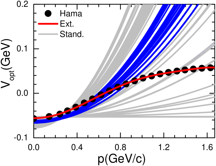
Figure 1: Single particle potential obtained from the standard Skyrme MDI (gray lines and blue lines) and the extended Skyrme MDI (red line). The points are the data of single particle potential obtained from Hama’s data [53].

To overcome the above deficiency of the standard Skyrme interaction, an extended Skyrme effective interaction that includes the terms in relative momenta up to sixth order was proposed in Refs. [48]. The extended Skyrme interaction was stimulated by the idea that it is possible to expand a finite range interaction in terms of a zero range like and such an expansion converges [56], and the central term can be written order by order as,

$$\begin{aligned} v_{\text{C}}&=t_{0}^{(0)}(1+x_{0}^{(0)}P_{\sigma})\delta(\mathbf{r})\\ &+\frac{1}{2}t_{1}^{(2)}(1+x_{1}^{(2)}P_{\sigma})\delta(\mathbf{r})[\mathbf{k}^{{}^{\prime}2}+\mathbf{k}^{2}]\\ &+t_{2}^{(2)}(1+x_{2}^{(2)}P_{\sigma})\delta(\mathbf{r})\mathbf{k}^{{}^{\prime}}\cdot\mathbf{k}\\ &+\frac{1}{4}t_{1}^{(4)}(1+x_{1}^{(4)}P_{\sigma})\delta(\mathbf{r})[(\mathbf{k}^{{}^{\prime}2}+\mathbf{k}^{2})^{2}+4(\mathbf{k}^{{}^{\prime}}\cdot\mathbf{k})^{2}]\\ &+t_{2}^{(4)}(1+x_{2}^{(4)}P_{\sigma})\delta(\mathbf{r})(\mathbf{k}^{{}^{\prime}}\cdot\mathbf{k})(\mathbf{k}^{{}^{\prime}2}+\mathbf{k}^{2})\\ &+\frac{t_{1}^{(6)}}{2}(1+x_{1}^{(6)}P_{\sigma})\delta(\mathbf{r})(\mathbf{k}^{{}^{\prime}2}+\mathbf{k}^{2})\\ &\quad[(\mathbf{k}^{{}^{\prime}2}+\mathbf{k}^{2})^{2}+12(\mathbf{k}^{{}^{\prime}}\cdot\mathbf{k})^{2}]\\ &+t_{2}^{(6)}(1+x_{2}^{(6)}P_{\sigma})\delta(\mathbf{r})(\mathbf{k}^{{}^{\prime}}\cdot\mathbf{k})[3(\mathbf{k}^{{}^{\prime}2}+\mathbf{k}^{2})^{2}+4(\mathbf{k}^{{}^{\prime}}\cdot\mathbf{k})^{2}].\end{aligned}$$ (7)

The first term in Eq.(7) is the local two-body interaction, the rest terms are the non-local interaction with the power of the relative momentum up to six, i.e., $\mathbf{k}^{6}$. $P_{\sigma}$ is the spin-exchange operator and $\mathbf{k}$ in Eq.(7) denotes the operator $(\mathbf{\nabla_{1}-\nabla_{2}})/2i$ acting on the right, whereas, $\mathbf{k^{{}^{\prime}}}$ is the operator $-(\mathbf{\nabla_{1}-\nabla_{2}})/2i$ acting on the left. They are related to the relative momentum between two nucleons.

Inspired by this idea, we assume a phenomenological momentum-dependent interaction as,

$$\begin{aligned} g(\mathbf{p}-\mathbf{p^{\prime}})&=\sum_{I=0}^{N}b_{I}(\mathbf{p}-\mathbf{p}^{\prime})^{2I}\end{aligned}$$ (8)

in the transport models. The parameter $b_{I}$ is used to determine the shape of the MDI, and its dimension is GeV^2-2I for keeping the dimension of $g(\mathbf{p}-\mathbf{p^{\prime}})$ in GeV². Consequently, the energy density $u_{md}$ in Eq.(6) is replaced by,

$$\begin{aligned} u_{md}&=\tilde{C}_{0}\sum_{ij}\int\text{d}^{3}p\text{d}^{3}p^{\prime}f_{i}(\mathbf{r},\mathbf{p})f_{j}(\mathbf{r},\mathbf{p^{\prime}})g(\mathbf{p}-\mathbf{p^{\prime}})\\ &\quad+\tilde{D}_{0}\sum_{ij\in n}\int\text{d}^{3}p\text{d}^{3}p^{\prime}f_{i}(\mathbf{r},\mathbf{p})f_{j}(\mathbf{r},\mathbf{p^{\prime}})g(\mathbf{p}-\mathbf{p^{\prime}})\\ &\quad+\tilde{D}_{0}\sum_{ij\in p}\int\text{d}^{3}p\text{d}^{3}p^{\prime}f_{i}(\mathbf{r},\mathbf{p})f_{j}(\mathbf{r},\mathbf{p^{\prime}})g(\mathbf{p}-\mathbf{p^{\prime}}).\end{aligned}$$ (9)

The number of $N$, the interaction parameters $b_{I}$, $\tilde{C}_{0}$ and $\tilde{D}_{0}$ in Eq.(8) and Eq.(9) can be determined by fitting the optical potential data or calculations from microscopic model, such as Dirac-Brueckner-Hartree-Fock[57]. At the given shape of MDI, i.e., given $N$ and $b_{I}$, one can vary the isoscalar effective mass and the isovector effective mass through $\tilde{C}_{0}$ and $\tilde{D}_{0}$.

In the following part, we will present the formulas for the single particle potential and the equation of state, the nuclear matter parameters and their relations to the interaction parameters in transport models and the Hamiltonian used in the QMD-type models as well.

II.1 Single particle potential and equation of state

The single particle potential $V_{q}$ can be calculated by taking the functional derivative of the energy density with respect to the single-body phase space distribution of protons or neutrons $f_{q}(r,p)$,

$$V_{q}(\rho,\delta,p) =\frac{\delta u_{\text{loc}}}{\delta f_{q}}+\frac{\delta u_{\text{md}}}{\delta f_{q}}$$ (10)

$$=V^{\text{loc}}_{q}(\rho,\delta)+V^{\text{md}}_{q}(\rho,\delta,p),$$

where q=n or p. The $V_{q}^{loc}$ is,

$$V^{\text{loc}}_{q}(\rho,\delta) =\frac{\delta u_{\text{loc}}}{\delta f_{q}}$$ (11)

$$=\alpha\frac{\rho}{\rho_{0}}+\beta\frac{\rho^{\gamma}}{\rho_{0}^{\gamma}}+(\gamma-1)B_{\text{sym}}\frac{\rho^{\gamma}}{\rho_{0}^{\gamma}}\delta^{2}$$

$$\quad\pm 2\left(A_{\text{sym}}\frac{\rho}{\rho_{0}}+B_{\text{sym}}\left(\frac{\rho}{\rho_{0}}\right)^{\gamma}\right)\delta.$$

The sign ‘$+$’ is for neutrons, and ‘$-$’ for protons.

The $V_{q}^{md}$ is,

$$\begin{aligned} V^{\text{md}}_{q}(\rho,\delta,p)&=\frac{\delta u_{\text{md}}}{\delta f_{q}}\\ &=2\tilde{C_{0}}\int d^{3}p^{{}^{\prime}}f(\mathbf{r},\mathbf{p^{\prime}})g(\mathbf{p}-\mathbf{p^{\prime}})\\ &\quad+2\tilde{D_{0}}\int d^{3}p^{{}^{\prime}}f_{q}(\mathbf{r},\mathbf{p^{\prime}})g(\mathbf{p}-\mathbf{p^{\prime}}).\end{aligned}$$ (12)

In the cold nuclear matter,

$$f_{q}(\mathbf{r},\mathbf{p^{\prime}}) = (\frac{4\pi}{3}p^{3}_{F_{q}})^{-1}\rho_{q}\Theta(p_{F_{q}}-|p^{\prime}|)$$

$$= \frac{2}{(2\pi\hbar)^{3}}\Theta(p_{F}-|p^{\prime}|),$$

and $p_{F_{q}}=\hbar(3\pi^{2}\rho_{q})^{\frac{1}{3}}$. Thus, the corresponding $V^{md}_{q}$ can also be written in an analytical form,

$$V^{\text{md}}_{q}(\rho,\delta,p) =2\tilde{C}_{0}\Bigg{[}\sum_{I=1}^{N}b_{I}\sum_{l=0,l\in even}^{2I}\mathcal{\tilde{A}}_{Il}\sum_{q=n,p}\rho_{q}^{(2I-l+3)/3}p^{l}\Bigg{]}$$ (14)

$$\quad+2\tilde{D}_{0}\Bigg{[}\sum_{I=1}^{N}b_{I}\sum_{l=0,l\in even}^{2I}\mathcal{\tilde{A}}_{Il}\rho_{q}^{(2I-l+3)/3}p^{l}\Bigg{]},$$

and,

$$\mathcal{\tilde{A}}_{Il} =\frac{2}{(2\pi\hbar)^{3}}4\pi\Bigg{[}\left(\hbar(3\pi^{2})^{1/3}\right)^{(2I-l+3)}\tbinom{2I}{l}\frac{1}{(2I-l+3)}\Bigg{]}.$$

Here, $\tbinom{2I}{l}$ represents the number of combinations of $l$ elements selected from $2I$ elements. One should note that the summation of $b_{I}$ in Eq.(14) starts from $b_{1}$. The value of $b_{0}$ will be related to the strength of the local potential when we use the extended Skyrme energy density functional.

Further, the single particle potential $V_{q}$ as in Eq.(10) can be expanded as a power series of isospin asymmetry $\delta$, by using the $\rho_{q}=\frac{\rho}{2}(1+\tau_{q}\delta)$, with $\tau_{q}=1$ or $-1$ for neutrons and protons. The so-called Lane potential[31] means one neglects the higher-order terms ($\delta^{2}$, $\delta^{3}$, $\cdots$), i.e.,

$$V_{q}=V_{0}\pm V_{asy}\delta+\cdots.$$ (15)

The $V_{0}$ is,

$$\begin{aligned} V_{0}&=\alpha\frac{\rho}{\rho_{0}}+\beta\frac{\rho^{\gamma}}{\rho_{0}^{\gamma}}+4(\tilde{C}_{0}+\frac{\tilde{D}_{0}}{2})\\ &\quad\times\Bigg{[}\sum_{I=1}^{N}b_{I}\sum_{l=0,l\in even}^{2I}\mathcal{\tilde{A}}_{Il}\times(\frac{\rho}{2})^{(2I-l+3)/3}\times p^{l}\Bigg{]}.\\ \end{aligned}$$ (16)

$V_{asy}$ is,

$$V_{asy} =2A_{\text{sym}}\frac{\rho}{\rho_{0}}+2B_{\text{sym}}\left(\frac{\rho}{\rho_{0}}\right)^{\gamma}$$ (17)

$$\quad+2\tilde{D}_{0}\Bigg{[}\sum_{I=1}^{N}b_{I}\sum_{l=0,l\in even}^{2I}\mathcal{\tilde{A}}_{Il}\frac{2I-l+3}{3}$$

$$\quad\quad\quad(\frac{\rho}{2})^{(2I-l+3)/3}p^{l}\Bigg{]}.$$

The first and second terms in Eq.(17) are the momentum-independent parts of the symmetry potential, and the last term is the momentum-dependent part of the symmetry potential.

The isospin asymmetric equation of state for cold nuclear matter reads,

$$E/A(\rho,\delta) =\frac{3\hbar^{2}}{10m}\left(\frac{3\pi^{2}}{2}\rho\right)^{2/3}+\frac{\alpha}{2}\frac{\rho}{\rho_{0}}+\frac{\beta}{\gamma+1}\frac{\rho^{\gamma}}{\rho^{\gamma}_{0}}$$ (18)

$$\quad+(\tilde{C}_{0}+\frac{\tilde{D}_{0}}{2})\sum_{I=1}^{N}\tilde{g}_{md}^{(I)}\times\rho^{2I/3+1}$$

$$\quad+S(\rho)\delta^{2}+\cdots$$

The coefficient of $\tilde{g}_{md}^{(I)}$ is,

$$\tilde{g}_{md}^{(I)} =\frac{4b_{I}}{2^{(2I+6)/3}}\sum_{l=0,l\in even}^{2I}\mathcal{G}_{Il},$$ (19)

with the $\mathcal{G}_{Il}$,

$$\mathcal{G}_{Il} =\left(\frac{2}{(2\pi\hbar)^{3}}\right)^{2}(4\pi)^{2}\Bigg{[}\left(\hbar(3\pi^{2})^{1/3}\right)^{(2I+6)}$$

$$\quad\tbinom{2I}{l}\frac{1}{(l+3)}\frac{1}{(2I-l+3)}\Bigg{]},$$

which has a constant value at given $I$ and $l$ and is independent of $b_{I}$.

The density dependence of the symmetry energy $S(\rho)$ becomes,

$$S(\rho) =\frac{\hbar^{2}}{6m}\left(\frac{3\pi^{2}\rho}{2}\right)^{2/3}+A_{\text{sym}}\frac{\rho}{\rho_{0}}+B_{\text{sym}}\left(\frac{\rho}{\rho_{0}}\right)^{\gamma}$$ (20)

$$\quad+\sum_{I=1}^{N}\tilde{C}_{sym}^{(I)}\rho^{2I/3+1}.$$

Here, the $\tilde{C}_{sym}^{(I)}$ is taken as

$$\tilde{C}_{sym}^{(I)} =2\tilde{C}_{0}\Bigg{[}\frac{b_{I}}{2^{(2I+6)/3}}\sum_{l=0,l\in even}^{2I}\mathcal{G}_{Il}$$ (21)

$$\quad\Big{(}\frac{l+3}{3}\frac{l}{3}+\frac{2I-l+3}{3}\frac{2I-l}{3}\Big{)}\Bigg{]}$$

$$\quad+\tilde{D}_{0}\Bigg{[}\frac{b_{I}}{2^{(2I+6)/3}}\frac{2I+6}{3}\frac{2I+3}{3}\sum_{l=0,l\in even}^{2I}\mathcal{G}_{Il}\Bigg{]}.$$

which is the I-th coefficient of the extended Skyrme-type MDI term in the symmetry energy.

The derivations of the energy density and the single particle potential can be found in Appendix A and Appendix B.

II.2 Nuclear matter parameters and its relation to the interaction parameters

The parameters used in the extended Skyrme interaction as in Eq.(18), i.e. $\alpha$, $\beta$, $\gamma$, $A_{sym}$, $B_{sym}$, $\tilde{C}_{0}$, and $\tilde{D}_{0}$, can be obtained from the nuclear matter parameters by the same standard protocol as in the standard Skyrme interaction[15]. They are realized by solving the seven equations for the determination of the saturation density $\rho_{0}$, the energy per nucleon at saturation density $E_{0}$, the incompressibility $K_{0}$, the isoscalar effective mass $m_{s}^{*}$, the isovector effective mass $m_{v}^{*}$, the symmetry energy coefficient $S(\rho_{0})$ and the slope of the symmetry energy $L$.

The first equation is related to the value of the saturation density $\rho_{0}$ which is obtained by seeking the root of the following equation,

$$P =\rho_{0}^{2}\frac{d}{d\rho}\frac{E}{A}(\rho_{0},\delta=0)=0,$$ (22)

i.e.,

$$\frac{2}{5}\epsilon_{F}^{0}\rho_{0}+\frac{\alpha}{2}\rho_{0}+\frac{\beta}{\gamma+1}\gamma\rho_{0}$$ (23)

$$\quad\quad+(\tilde{C}_{0}+\frac{\tilde{D}_{0}}{2})\sum_{I=1}^{N}\tilde{g}_{md}^{(I)}\left(\frac{2I}{3}+1\right)\rho_{0}^{2I/3+2}=0,$$

here, $\epsilon_{F}^{0}=\frac{\hbar^{2}}{2m}\left(\frac{3\pi^{2}\rho_{0}}{2}\right)^{2/3}$.

The second equation is the binding energy $E_{0}$. It reads,

$$E_{0} =E/A(\rho_{0})$$ (24)

$$=\frac{3}{5}\epsilon_{F}^{0}+\frac{\alpha}{2}+\frac{\beta}{\gamma+1}+(\tilde{C}_{0}+\frac{\tilde{D}_{0}}{2})\sum_{I=1}^{N}\tilde{g}_{md}^{(I)}\rho_{0}^{2I/3+1}.$$

The third equation is the incompressibility $K_{0}$, i.e.,

$$K_{0} =9\rho_{0}^{2}\frac{\partial^{2}E/A}{\partial\rho^{2}}|_{\rho_{0}}$$ (25)

$$=\frac{-6}{5}\epsilon_{F}^{0}+9\frac{\beta}{\gamma+1}\gamma(\gamma-1)$$

$$\quad+6(\tilde{C}_{0}+\frac{\tilde{D}_{0}}{2})\sum_{I=1}^{N}\tilde{g}_{md}^{(I)}\left(\frac{2I}{3}+1\right)I\rho_{0}^{2I/3+1}.$$

The fourth and fifth equations are related to the neutron/proton effective mass or the isoscalar and isovector effective mass. The neutron/proton effective mass is obtained from the neutron/proton potential according to,

$$\frac{m}{m_{q}^{*}}=1+\frac{m}{p}\frac{\partial V_{q}}{\partial p},\quad q=n,p.$$ (26)

The neutron/proton effective mass will be,

$$\frac{m}{m_{q}^{*}} =1+2\tilde{C}_{0}m\Bigg{[}\sum_{I=1}^{N}b_{I}\sum_{l=0,l\in even}^{2I}\mathcal{\tilde{A}}_{Il}$$ (27)

$$\quad\sum_{q}\rho_{q}^{(2I-l+3)/3}l\times p^{l-2}\Bigg{]}$$

$$\quad+2\tilde{D}_{0}m\Bigg{[}\sum_{I=1}^{N}b_{I}\sum_{l=0,l\in even}^{2I}\mathcal{\tilde{A}}_{Il}$$

$$\quad\quad\rho_{q}^{(2I-l+3)/3}l\times p^{l-2}\Bigg{]}.$$

Then, we can find the relationship between $\Delta m_{np}^{*}=(m_{n}^{*}-m_{p}^{*})/m$ and $V_{asy}$ as

$$\Delta m_{np}^{*}\approx-(\frac{m^{*}}{m})^{2}4m\delta\frac{\partial V_{asy}}{\partial p^{2}},$$ (28)

The derivation can be found in AppendixC. It means that the strength of the effective mass splitting $\Delta m_{np}^{*}$ depends on the momentum-dependent part of the symmetry potential when the $m^{*}/m$ is fixed.

The isoscalar effective mass $m_{s}^{*}$ can be obtained at $\rho_{q}=\rho/2$ from Eq. (27), and the isovector effective mass $m_{v}^{*}$ can be obtained at $\rho_{q}=0$ which represents the neutron(proton) effective mass in pure proton(neutron) matter as in Refs. [58, 59]. They are,

$$\frac{m}{m_{s}^{*}}(\rho,p) =1+4(\tilde{C}_{0}+\frac{\tilde{D}_{0}}{2})m\Bigg{[}\sum_{I=1}^{N}b_{I}\sum_{l=0,l\in even}^{2I}\mathcal{\tilde{A}}_{Il}$$ (29)

$$\quad(\frac{\rho}{2})^{(2I-l+3)/3}l\times p^{l-2}\Bigg{]},$$

$$\frac{m}{m_{v}^{*}}(\rho,p) =1+4\tilde{C}_{0}m\Bigg{[}\sum_{I=1}^{N}b_{I}\sum_{l=0,l\in even}^{2I}\mathcal{\tilde{A}}_{Il}$$

$$\quad(\frac{\rho}{2})^{(2I-l+3)/3}l\times p^{l-2}\Bigg{]}.$$

As same as in Ref.[27], we define a quantity ${f}_{I}$,

$${f}_{I}(\rho,p) =\frac{m}{m_{s}^{*}}-\frac{m}{m_{v}^{*}}$$ (30)

$$=2\tilde{D}_{0}m\Bigg{[}\sum_{I=1}^{N}b_{I}\sum_{l=0,l\in even}^{2I}\mathcal{\tilde{A}}_{Il}$$

$$\quad(\frac{\rho}{2})^{(2I-l+3)/3}l\times p^{l-2}\Bigg{]},$$

to describe the isospin effective mass splitting, which has the opposite sign with $\Delta m_{np}^{*}$. In practical transport model calculations, $\Delta m_{np}^{*}$ depends on the power expansion of isospin asymmetry and can not be used to calculate the $\tilde{D}_{0}$ accurately. Thus, in the determination of interaction parameters in the transport models, we use the values of $m_{s}^{*}/m$ and $f_{I}$.

The sixth and seventh equations are the symmetry energy coefficient $S_{0}$,

$$S_{0} =S(\rho_{0})$$ (31)

$$=\frac{1}{3}\epsilon_{F}^{0}+A_{sym}+B_{sym}+\sum_{I=1}^{N}\tilde{C}_{sym}^{(I)}\rho_{0}^{2I/3+1},$$

and the slope of the symmetry energy $L$ is,

$$L =3\rho_{0}\frac{\partial S(\rho)}{\partial\rho}|_{\rho_{0}}$$ (32)

$$=\frac{2}{3}\epsilon_{F}^{0}+3A_{sym}+3B_{sym}\gamma$$

$$\quad+3\sum_{I=1}^{N}\tilde{C}_{sym}^{(I)}\left(\frac{2I}{3}+1\right)\rho_{0}^{2I/3+1}.$$

Given the values $S_{0}$, $L$, $K_{0}$, $E_{0}$ and $\rho_{0}$, ${f}_{I}^{0}={f}_{I}(\rho_{0},p_{F})$ and $\frac{m}{m_{s0}^{*}}=\frac{m}{m_{s}^{*}}(\rho_{0},p_{F})$, the coefficients $\alpha$, $\beta$, $\gamma$, $A_{sym}$, $B_{sym}$, $\tilde{C}_{0}$ and $\tilde{D}_{0}$ can be obtained according to the following formulas.

$$\tilde{D}_{0} ={f}_{I}^{0}/\Bigg{[}2m\sum_{I=1}^{N}b_{I}\sum_{l=0,l\in even}^{2I}\mathcal{\tilde{A}}_{Il}$$ (33)

$$\quad\quad\quad(\frac{\rho_{0}}{2})^{(2I-l+3)/3}l\times p_{F}^{l-2}\Bigg{]}.$$

$$\tilde{C}_{0} =(\frac{m}{m_{s0}^{*}}-1)/\Bigg{[}4m\sum_{I=1}^{N}b_{I}\sum_{l=0,l\in even}^{2I}$$ (34)

$$\quad\quad\mathcal{\tilde{A}}_{Il}(\frac{\rho_{0}}{2})^{(2I-l+3)/3}l\times p_{F}^{l-2}\Bigg{]}-\frac{\tilde{D}_{0}}{2}.$$

$$\gamma=\frac{K_{0}+\frac{6}{5}\epsilon_{F}^{0}-6(\tilde{C}_{0}+\frac{\tilde{D}_{0}}{2})\sum_{I=1}^{N}(\frac{2I}{3}+1)I\rho_{0}^{\frac{2I}{3}+1}\tilde{g}_{md}^{(I)}}{\frac{9}{5}\epsilon_{F}^{0}-6(\tilde{C}_{0}+\frac{\tilde{D}_{0}}{2})\sum_{I=0}^{N}I\rho_{0}^{\frac{2I}{3}+1}\tilde{g}_{md}^{(I)}-9E_{0}},$$ (35)

$$\beta=\frac{(\frac{1}{5}\epsilon_{F}^{0}-\frac{2}{3}(\tilde{C}_{0}+\frac{\tilde{D}_{0}}{2})\sum_{I=1}^{N}I\rho_{0}^{\frac{2I}{3}+1}\tilde{g}_{md}^{(I)}-E_{0})(\gamma+1)}{\gamma-1},$$

$$\alpha=2E_{0}-2(\tilde{C}_{0}+\frac{\tilde{D}_{0}}{2})\sum_{I=1}^{N}\rho_{0}^{\frac{2I}{3}+1}\tilde{g}_{md}^{(I)}-\frac{6}{5}\epsilon_{F}^{0}-\frac{2\beta}{\gamma+1},$$

$$B_{sym}=\frac{3S_{0}-L-\frac{1}{3}\epsilon_{F}^{0}+2\sum_{I=1}^{N}I\tilde{C}_{sym}^{(I)}\rho_{0}^{\frac{2I}{3}+1}}{-3(\gamma-1)},$$

$$A_{sym}=S_{0}-\frac{1}{3}\epsilon_{F}^{0}-B_{sym}-\sum_{I=1}^{N}\tilde{C}_{sym}^{(I)}\rho_{0}^{\frac{2I}{3}+1}.$$

The advantages of using nuclear matter parameters as input are as similar as in Ref. [60]. Simply, the nuclear matter parameters have a precise physical meaning. Then, it is easy to do the Bayesian analysis in transport model simulations in the nuclear matter parameter space, and the culmination of the optimization procedure provides theoretical predictions for all bulk properties with meaningful error bars.

II.3 Hamiltonian from extended Skyrme MDI in the quantum molecular dynamics type models

Here, we give an example of the Hamiltonian of the extend Skyrme MDI in the QMD-type models. The energy density of the extended Skyrme MDI can be obtained by folding the interaction with the wave function or with the phase space density as in Eq.(9).

In the framework of the ImQMD model, the result of the integration term $I_{ij}=\int\text{d}^{3}p\text{d}^{3}p^{\prime}f_{i}(\mathbf{r},\mathbf{p})f_{j}(\mathbf{r},\mathbf{p^{\prime}})g(\mathbf{p}-\mathbf{p^{\prime}})$ in Eq.(9) is,

$$I_{ij}=\int\text{d}^{3}p\text{d}^{3}p^{\prime}f_{i}(\mathbf{r},\mathbf{p})f_{j}(\mathbf{r},\mathbf{p^{\prime}})g(\mathbf{p}-\mathbf{p^{\prime}})$$ (36)

$$=\frac{1}{(2\pi\sigma_{r}^{2})^{3}}\frac{1}{(\pi\sigma_{p}^{2})^{1/2}}\exp{[-\frac{(\mathbf{r}-\mathbf{r}_{i})^{2}}{2\sigma_{r}^{2}}-\frac{(\mathbf{r}-\mathbf{r}_{j})^{2}}{2\sigma_{r}^{2}}]}$$

$$\quad\sum_{I=1}^{N}b_{I}\sum_{l=0,l\in even}^{2I+1}\tbinom{2I+1}{l}(\mathbf{p}_{i}-\mathbf{p}_{j})^{2I-l}W(l,\sigma_{p}).$$

Here, $W(l,\sigma_{p})$ are the contributions from the width of the wave packet and they are,

$$W(0,\alpha=1/4\sigma_{p}^{2}) =\frac{\sqrt{\pi}}{2\alpha^{1/2}}=\sqrt{\pi}\sigma_{p},$$ (37)

$$W(1,\alpha=1/4\sigma_{p}^{2}) =\frac{1}{2\alpha}=2\sigma_{p}^{2},$$

$$\cdots,$$

$$W(l,\alpha=1/4\sigma_{p}^{2}) =-\frac{\partial}{\partial\alpha}W(l-2,\sigma_{p}).$$

The integration of $I_{ij}$ over the coordinate space is,

$$\int I_{ij}d^{3}r=$$ (38)

$$\quad\rho_{ij}\sum_{I=1}^{N}b_{I}\sum_{l=0,l\in even}^{2I+1}\tbinom{2I+1}{l}(\mathbf{p}_{i}-\mathbf{p}_{j})^{2I-l}\frac{{W}(l,\sigma_{p})}{(\pi\sigma_{p}^{2})^{1/2}},$$

and thus the corresponding part of Hamiltonian is,

$$\begin{aligned} H&=2\tilde{C}_{0}\sum_{ij}\rho_{ij}\sum_{I=1}^{N}b_{I}\sum_{l=0,l\in even}^{2I+1}\tbinom{2I+1}{l}(\mathbf{p}_{i}-\mathbf{p}_{j})^{2I-l}\\ &\quad\quad\times\frac{{W}(l,\sigma_{p})}{(\pi\sigma_{p}^{2})^{1/2}}\\ &\quad+(\tilde{C}_{0}+\tilde{D}_{0})\sum_{ij\in q}\rho_{ij}\sum_{I=1}^{N}b_{I}\sum_{l=0,l\in even}^{2I+1}\tbinom{2I+1}{l}\\ &\quad\quad\times(\mathbf{p}_{i}-\mathbf{p}_{j})^{2I-l}\frac{{W}(l,\sigma_{p})}{(\pi\sigma_{p}^{2})^{1/2}},\\ \end{aligned}$$ (39)

here,

$$\rho_{ij}=\frac{1}{(4\pi\sigma_{r}^{2})^{3/2}}\text{exp}[-\frac{(\mathbf{r_{i}}-\mathbf{r_{j}})^{2}}{4\sigma_{r}^{2}}].$$ (40)

III Results and discussions

III.1 Determination of the expansion number $N$ and coefficient $b_{I}$

The values of $N$, $b_{I}$, $\tilde{C}_{0}$ and $\tilde{D}_{0}$ are obtained by fitting the $V_{0}$($\rho_{0}$, $p$) in Eq.(16) to Hama’s optical potential data [53], which gives the isoscalar effective mass $m_{s}^{*}/m=0.77$. One should note that the data can be well described when N$\geq$4. As an example, we present the fitting results with extended Skyrme MDI in Fig. 1 as the red line. The values of $b_{I}$, $\tilde{C}_{0}$ and $\tilde{D}_{0}$ for $N=4$, 5 and 6 are listed in Table1. Our calculations show that the results of EOS, single particle potential, and HIC observables, are independent of the $N$ we used, since they are used to fit the same data. In the following calculations, we will keep $N=4$ and the values of $b_{1}$ to $b_{4}$ are fixed. Nevertheless, the extrapolated strength of the single particle potential above 1 GeV is different for different $N$, and which should be investigated by using the HICs at high beam energies[61] and will not be discussed in this paper.

Table 1: The parameters of $b_{I}$ used in extended Skyrme MDI are in GeV^2-2I and $\tilde{C}_{0}$, $\tilde{D}_{0}$ are $\rm{fm}^{3}\rm{GeV}^{-1}$.

N	$b_{0}$	$b_{1}$	$b_{2}$	$b_{3}$	$b_{4}$	$b_{5}$	$b_{6}$	$\tilde{C}_{0}$	$\tilde{D}_{0}$
4	-1.105	3.649	-2.608	0.826	-0.093	-	-	0.182	0.00
5	-1.135	4.137	-3.821	1.837	-0.428	0.038	-	0.182	0.00
6	-1.149	4.434	-4.828	3.048	-1.070	0.193	-0.014	0.182	0.00

III.2 Single particle potential, equation of state and symmetry energy

Now, let us check the single particle potential, the symmetric equation of state and the symmetry energy obtained with the extended Skyrme MDI. For comparisons, we also plot the corresponding results obtained with the standard Skyrme MDI. In the calculations, we fix the values of $K_{0}=230$ MeV, $m_{s}^{*}/m=0.77$, $S_{0}=32$ MeV and vary the $L$ and the $f_{I}$. In Table 2, we list the corresponding interaction parameters, such as $\alpha$, $\beta$, $\gamma$, $A_{sym}$, $B_{sym}$, $\tilde{C}_{0}$ and $\tilde{D}_{0}$, that will be used in the transport models. The values in brackets from the second to the eighth rows represent the values obtained with the standard Skyrme MDI as in Ref. [15].

Table 2: The parameters used in the calculations corresponding to $K_{0}=230$ MeV, $m_{s}^{*}/m=0.77$, $S_{0}=32$ MeV, and different values of $L$ and $f_{I}$. The parameters $\alpha$, $\beta$, $A_{sym}$, $B_{sym}$ are in MeV. $\tilde{C}_{0}$ and $\tilde{D}_{0}$ are $\rm{fm}^{3}\rm{GeV}^{-1}$.

Para.	(L=46, $f_{I}$=0.3)	(L=46, $f_{I}$=-0.3)	(L=100, $f_{I}$=0.3)	(L=100, $f_{I}$=-0.3)
$\alpha$	-236.58 (-265.78)
$\beta$	163.95 (194.93)
$\gamma$	1.26 (1.22)
$A_{sym}$	83.65 (108.44)	58.57 (62.73)	14.41 (25.32)	-10.67 (-20.40)
$B_{sym}$	-79.48 (-103.69)	-30.52 (-35.38)	-10.25 (-20.34)	38.72 (47.96)
$\tilde{C}_{0}$	$-7.92\times 10^{-4}$ ($-2.08\times 10^{-3}$)	0.37 (1.00)	$-7.92\times 10^{-4}$ ($-2.08\times 10^{-3}$)	0.37 (1.00)
$\tilde{D}_{0}$	0.37 (1.00)	-0.37 (-1.00)	0.37 (1.00)	-0.37 (-1.00)

Figure LABEL:eos (a) presents the equation of state of symmetric nuclear matter with the parameters we used. The gray lines are the EOS obtained by the 123 standard Skyrme interaction sets. It shows that the extended Skyrme interaction can reasonably reproduce the EOS for symmetric nuclear matter, and avoid the defect of describing EOS by only using the Taylor expansion parameters as described in Ref.[62].

The panel (b) is the density dependence of the symmetry energy obtained with the extended Skyrme MDI (coloured lines) and the standard Skyrme MDI (gray lines). As expected, the results obtained with different $L$ exhibit different density dependence of the symmetry energy. However, the influence of different $f_{I}$ on the density dependence of the symmetry energy is weak. For the standard Skyrme MDI (gray lines), the influence of different $f_{I}$ mainly appears at the density above 1.5$\rho_{0}$. At $\rho=2\rho_{0}$, the difference between the symmetry energy obtained with two $f_{I}$ is less than 7% for $L=100$ MeV, and is less than 13% for $L=46$ MeV. For extended Skyrme MDI, the density dependence of the symmetry energy obtained with $f_{I}=0.3$ (solid lines) and $f_{I}=-0.3$ (dashed lines) are close to each other at both $L=46$ or 100 MeV at $\rho<3\rho_{0}$. The reason is that the different effective mass splitting obtained by the extended Skyrme MDI have a smaller impact on the $A_{sym}$, $B_{sym}$, and $C_{sym}^{(I)}$ terms in the density dependent of the symmetry energy compared to the standard Skyrme MDI according to the Eq.(33)-Eq.(35).

Based on the above discussions, one can expect the symmetry energy constraints from the properties of the neutron stars, such as the mass-radius relationship and the tidal deformability, can not well distinguish $f_{I}$ (or effective mass splitting $\Delta m_{np}^{*}$), because the Tolman-Oppenheimer-Volkov (TOV) equation of neutron stars only depends on the pressure vs density [63]. However, the similar density-dependent symmetry energy from different $f_{I}$ could lead to different effects on the HICs observables via the momentum dependent symmetry potential, and thus the constraints of the symmetry energy from HICs may be different from the constraints from neutron stars.

Figure LABEL:fig:VLane (a) and (b) present the neutron potential $V_{n}$ (black lines) and the proton potential $V_{p}$ (red lines) as functions of the kinetic energy $E_{k}$ in nuclear matter at $\rho=\rho_{0}$ and $\delta=0.2$. The dashed lines are obtained with the standard Skyrme MDI, and the solid lines are obtained with the extended Skyrme MDI.

As expected, the values of $V_{n}$ and $V_{p}$ obtained from the extended Skyrme MDI do not follow the straight increase as that given by the standard Skyrme interaction but bend and then become flat with an increase of $E_{k}$. When $f_{I}=0.3$ ($m_{n}^{*}<m_{p}^{*}$), the $V_{n}$ is greater than $V_{p}$. More details, the neutrons will feel a stronger repulsive force than protons at high kinetic energy where $V_{q}>0$, and the neutrons feel a weaker attractive force than protons at low kinetic energy where $V_{q}<0$. For $f_{I}=-0.3$ ($m_{n}^{*}>m_{p}^{*}$), $V_{n}$ is less than $V_{p}$ at $E_{k}>150$ MeV and a contradictory behavior is observed at $E_{k}<150$ MeV. To single out the contributions from the isoscalar single particle potential, the symmetry potentials $V_{sym}$ as functions of kinetic energy $E_{k}$ are plotted in panel (c). The convention of the line styles is as same as in panel (a) and (b). The green and blue lines represent $f_{I}=-0.3$ and $f_{I}=+0.3$, respectively. The $V_{sym}$ increases (decreases) with the kinetic energy increasing for $f_{I}=+0.3$ ($f_{I}=-0.3$). Different than the standard Skyrme MDI, the values of $V_{sym}$ obtained from the extended Skyrme MDI tend to flatten out as $E_{k}$ increases. Thus, one may expect the difference of the neutron to proton yield ratios in HICs, i.e., $Y(n)/Y(p)$, obtained from two different $f_{I}$ will become smaller for the extended Skyrme MDI than that for standard Skyrme interaction.

III.3 The effects of extended Skyrme MDI on the neutron to proton ratios

To see the influence by using the extended Skyrme MDI and the standard Skyrme MDI on the HICs observables, the central collisions of the systems $A=^{124}$Sn+¹²⁴Sn and $B=^{112}$Sn+¹¹²Sn are simulated at the beam energy of 120 MeV/u. The HIC observables, i.e., the single ratio of the coalescence invariant (CI) neutron and proton $R_{n/p}=Y_{CI}(n)/Y_{CI}(p)$ and the double ratio of the coalescence invariant (CI) neutron and proton $DR(n/p)=R_{n/p}(A)/R_{n/p}(B)$, are analyzed under different $L$ and $f_{I}$. The $Y_{CI}(n)$ and $Y_{CI}(p)$ are obtained by combining the free nucleons with those bound in light isotopes with $1<A<5$[64, 65].

In Figure LABEL:NPratio-E120, we present the $R_{n/p}$ and $DR(n/p)$ as a function of $E_{k}/A$, i.e., the kinetic energy per nucleon of emitted particles in the center of mass frame. The left and middle panels are $R_{n/p}$ for ¹¹²Sn+¹¹²Sn and ¹²⁴Sn+¹²⁴Sn, respectively. The right panels are for the $DR(n/p)$. Our calculations show that the values of $R_{n/p}$ and $DR(n/p)$ obtained with $f_{I}=0.3$ are greater than that with $f_{I}=-0.3$ at high kinetic energy region for both MDIs (shaded regions) and both $L$ (the results for $L=46$ MeV are in the upper panels and the results for $L=100$ MeV are in the bottom panels). It can be understood from the symmetry potential presented in Fig.LABEL:fig:VLane.

To understand the difference of the $R_{n/p}$ (or $DR(n/p)$) obtained with two MDIs, we also present the results obtained with standard Skyrme MDI in the dashed shaded regions. The values of $R_{n/p}$ obtained with the extended Skyrme-type MDI are almost the same as those obtained with the standard Skyrme MDI in the low kinetic energy region where the symmetry potential of the two MDI forms is basically the same. At the high kinetic energy region, the $R_{n/p}$ obtained with the extended Skyrme MDI is different than that with standard Skyrme MDI, but the difference depends on the $f_{I}$. In the case of $f_{I}=-0.3$, the $R_{n/p}$ obtained with extended Skyrme MDI are obviously larger than that with standard Skyrme MDI. But for $f_{I}=0.3$, the $R_{n/p}$ obtained with extended Skyrme MDI are close to that with standard Skyrme MDI. It seems contradictory with the symmetry potential presented in Fig.LABEL:fig:VLane, but can be understood from the reaction dynamics.

In the simulations of HICs, the maximum compressed density depends on the form of MDI as shown in Fig.LABEL:fig:Vsym-rho (a). For $f_{I}=-0.3$, our calculations show that the maximum compressed density reaches about 1.94$\rho_{0}$ for extended Skyrme MDI and reaches about 1.84$\rho_{0}$ for standard Skyrme MDI. The difference of the maximum compressed density obtained with two MDIs is less than 6%. Thus, the difference of $R_{n/p}$ obtained with two MDIs will be similar with the difference of symmetry potential at a certain density. However, for $f_{I}=0.3$, the difference of the maximum compressed density obtained with two MDIs reaches about 18%, where the maximum compressed density reaches about 1.9$\rho_{0}$ for extended Skyrme MDI and reaches about 1.56$\rho_{0}$ for standard Skyrme MDI. Consequently, the difference of $R_{n/p}$ obtained with two MDIs will not be similar with the difference of symmetry potential at a certain density. It will be like a difference of the symmetry potential at two densities for two MDIs. For example, as shown in Fig.LABEL:fig:Vsym-rho (b), the difference of the symmetry potential obtained with the extended Skyrme MDI at 1.5$\rho_{0}$ and the symmetry potential obtained with the standard Skyrme MDI at 1.0$\rho_{0}$ is small, and thus the difference of $R_{n/p}$ between two MDIs becomes smaller for $f_{I}=0.3$.

III.4 Discussions on the constraints of the effective mass splitting

Further, we also compare the calculation to the corrected data of $R_{n/p}$ and $DR(n/p)$ (green symbols) that were published in Ref. [65]. In general, the calculated $R_{n/p}$ is close to the data. The $DR_{n/p}$ obtained with $f_{I}=-0.3(\Delta m_{np}^{*}\approx 0.311\delta)$ are close to the data points for $L=46$ MeV. In the case of $L=100$ MeV, the data falls into the middle between the results obtained with $f_{I}=-0.3(\Delta m_{np}^{*}\approx 0.311\delta)$ and $f_{I}=0.3(-\Delta m_{np}^{*}\approx 0.311\delta)$. It implies that the $\Delta m_{np}^{*}$ is negatively correlated to the $L$ and which is consistent with the results obtained with Hugenholtz-Van Hove (HVH) theorem [66]. This conclusion is consistent with the previous results in Ref.[65]. However, one should note that the $DR(n/p)$ suppresses the sensitivity to effective mass splitting, and the curves of $R_{n/p}$ as a function of $E_{k}$ are different than the data for both reaction systems if we carefully check its shape. Therefore, it is important to further quantitatively analyze the shapes of $R_{n/p}$ as a function of $E_{k}$.

To probe the strength of the effective mass splitting which only depends on the momentum-dependent part of the symmetry potential (as mentioned in Eq.(28)), one has to single out the contributions from the momentum-dependent part of the symmetry potential. The slope of $\ln{R_{n/p}}$ as a function of $E_{k}/A$, i.e.,

$$S_{n/p}=\frac{\partial\ln{R_{n/p}}}{\partial E_{k}/A},$$ (41)

can be used as mentioned in Ref. [33]. According to the statistical and dynamical model [67, 68, 69, 70, 71, 72], the neutron to proton yield ratios $R_{n/p}$ can be written as,

$$R_{n/p}=\frac{\text{Y(n)}}{\text{Y(p)}} \propto\exp\left(\frac{\mu_{n}-\mu_{p}}{T}\right)=\exp\left(\frac{2V_{asy}\delta}{T}\right).$$ (42)

$T$ is the temperature of the emitting source, $\mu_{n}$ and $\mu_{p}$ are the chemical potentials of neutrons and protons, respectively. If we expand the symmetry potential with respect to $p^{2}$, i.e., $V_{asy}=V_{asy}^{0}+\frac{\partial V_{asy}}{\partial p^{2}}p^{2}+\cdots$, then $R_{n/p}$ can be written as,

$$R_{n/p} \propto\exp\Bigg{[}\frac{2(V_{asy}^{0}+\frac{\partial V_{asy}}{\partial p^{2}}p^{2}+\cdots)\delta}{T}\Bigg{]}$$ (43)

$$\approx\exp\Bigg{[}\frac{2V_{asy}^{0}\delta}{T}\Bigg{]}\exp\Bigg{[}-\frac{(\frac{m}{m^{*}})^{2}\Delta m_{np}^{*}}{T}E^{\prime}_{k}\Bigg{]}.$$

$E^{\prime}_{k}=p_{rel}^{2}/2m$ is the relative kinetic energy between colliding nucleon pairs during the collisions, which should positively correlate to the kinetic energy of emitted nucleons. If we simply assume $E^{\prime}_{k}=\lambda E_{k}/A$, then we have

$$S_{n/p}=-\frac{\lambda}{T}(\frac{m}{m^{*}})^{2}\Delta m_{np}^{*},$$ (44)

which is directly related to the $\Delta m_{np}^{*}$. If one assumes $\lambda=1$ and $T=5$ MeV, the estimated values of $S_{n/p}$ are in the range from $\pm 0.02$ for the parameters we used, i.e., $m_{s}^{*}/m=0.77$ and $f_{I}=\pm 0.3$. In the HICs, the $\lambda$ is related to the friction of the system and the value should be smaller than one. Thus, one can expect the $|S_{n/p}|<0.02$ if $T=5$ MeV.

In Figure LABEL:fig:Snp, we present the $S_{n/p}$ obtained in the simulation and data. Two kinetic regions, i.e., the kinetic energy per nucleon of the emitted particles in the range of 35MeV $\leq\Delta E_{1}\leq$ 55MeV and 55MeV $\leq\Delta E_{2}\leq$ 95MeV, are used to calculate $S_{n/p}$. The systems of ¹¹²Sn+¹¹²Sn and ¹²⁴Sn+¹²⁴Sn at the beam energy of 120 MeV/u are presented in the left and right panels, respectively. The red circles represent the results obtained with $f_{I}=0.3$, the blue circles represent the results with $f_{I}=-0.3$. The green squares are the data points of $S_{n/p}$ which are extracted from the published experimental data [65]. One can find that the calculations tend to favor different effective mass splitting at different kinetic energy regions. In quality, the calculated values of $S_{n/p}$ tend to favor $f_{I}<0$ ($m_{n}^{*}>m_{p}^{*}$) at the kinetic energy less than 55 MeV. At the kinetic energy greater than 55 MeV, the calculated values of $S_{n/p}$ tend to favor $f_{I}>0$ ($m_{n}^{*}<m_{p}^{*}$). It implies the $m_{n}^{*}>m_{p}^{*}$ at low kinetic energy and $m_{n}^{*}<m_{p}^{*}$ at high kinetic energy, which is consistent with the theoretical calculations from the relativistic Hartree-Fock calculations[73]. In quantity, the calculations can not describe the shape of $R_{n/p}$ by the parameter sets we used. The possible reasons may be a reasonable parameter set is not used or the cluster formation for light particles is not well described. To rule out the first reason, a systematic analysis of $R_{n/p}$ on the multi-dimensional parameter space is certainly needed before going to understand the cluster formation mechanism and draw a firm conclusion on the effective mass splitting.

IV SUMMARY

The main goal of this work is to obtain an extended Skyrme momentum-dependent interaction, mean field potential and Hamiltonian, which can be easily used in both the BUU and QMD-type models for simulating the heavy ion collisions at intermediate to high energies. Especially, it can treat the width of the wave packet explicitly in the QMD-type Hamiltonian, and is flexible to adjust the strength of the momentum-dependent symmetry potential to investigate the effective mass splitting in transport models. In another, the relationship between the nuclear matter parameters and the interaction parameters used in the transport models are provided, which makes the transport model investigate the nuclear matter parameter in multidimensional parameter space easily.

As an example, we apply the extended Skyrme MDI to the ImQMD model. The isospin sensitive observables, such as the single and double ratios of the coalescence neutron to proton yields ($R_{n/p}$ and $DR(n/p)$), for ^112,124Sn+^112,124Sn at the beam energy of 120 MeV/u are analyzed to understand the influence of effective mass splitting. Our calculations show that the difference of the $R_{n/p}$ ratios obtained with two different strengths of the effective mass splitting, i.e. $f_{I}=+0.3$ and $f_{I}=-0.3$, becomes weaker for the extended Skyrme MDI than that for the standard Skyrme MDI.

To probe the strength of the effective mass splitting, the slope of $\ln{R_{n/p}}$ as a function of $E_{k}/A$, i.e., $S_{n/p}=\frac{\partial\ln{R_{n/p}}}{\partial E_{k}/A}$, is proposed and used. Our calculations show that $S_{n/p}$ is directly related to the effective mass splitting $\Delta m_{np}^{*}$. By comparing $S_{n/p}$ with the experimental data, in quality, one can find that the calculations favor different effective mass splitting at different kinetic energy regions. The calculated values of $S_{n/p}$ tend to favor $m_{n}^{*}>m_{p}^{*}$ at the kinetic energy less than 55 MeV and tend to favor $m_{n}^{*}<m_{p}^{*}$ at the kinetic energy greater than 55 MeV. In quantity, the calculations can not accurately describe the shape of $R_{n/p}$ by the parameter sets we used. Thus, further analysis on the $R_{n/p}$ in multi-dimensional parameter space is certainly needed to understand the discrepancy and to reliably constrain the effective mass splitting.

Appendix A Energy density of the extended Skyrme-type momentum-dependent interaction

Extended Skyrme-type MDI energy density is:

$$\begin{aligned} u_{md}&=\tilde{C}_{0}\int\text{d}^{3}p\text{d}^{3}p^{\prime}f(\mathbf{r},\mathbf{p})f(\mathbf{r},\mathbf{p^{\prime}})g(\mathbf{p}-\mathbf{p^{\prime}})\\ &\quad+\tilde{D}_{0}\int\text{d}^{3}p\text{d}^{3}p^{\prime}f_{n}(\mathbf{r},\mathbf{p})f_{n}(\mathbf{r},\mathbf{p^{\prime}})g(\mathbf{p}-\mathbf{p^{\prime}})\\ &\quad+\tilde{D}_{0}\int\text{d}^{3}p\text{d}^{3}p^{\prime}f_{p}(\mathbf{r},\mathbf{p})f_{p}(\mathbf{r},\mathbf{p^{\prime}})g(\mathbf{p}-\mathbf{p^{\prime}}).\\ &=\tilde{C}_{0}\int\text{d}^{3}p\text{d}^{3}p^{\prime}\\ &\quad\Bigg{(}f_{n}(\mathbf{r},\mathbf{p})f_{n}(\mathbf{r},\mathbf{p^{\prime}})+f_{n}(\mathbf{r},\mathbf{p})f_{p}(\mathbf{r},\mathbf{p^{\prime}})\\ &\quad+f_{p}(\mathbf{r},\mathbf{p})f_{n}(\mathbf{r},\mathbf{p^{\prime}})+f_{p}(\mathbf{r},\mathbf{p})f_{p}(\mathbf{r},\mathbf{p^{\prime}})\Bigg{)}g(\mathbf{p}-\mathbf{p^{\prime}})\\ &\quad+\tilde{D}_{0}\int\text{d}^{3}p\text{d}^{3}p^{\prime}f_{n}(\mathbf{r},\mathbf{p})f_{n}(\mathbf{r},\mathbf{p^{\prime}})g(\mathbf{p}-\mathbf{p^{\prime}})\\ &\quad+\tilde{D}_{0}\int\text{d}^{3}p\text{d}^{3}p^{\prime}f_{p}(\mathbf{r},\mathbf{p})f_{p}(\mathbf{r},\mathbf{p^{\prime}})g(\mathbf{p}-\mathbf{p^{\prime}}).\\ \end{aligned}$$ (45)

and $g(\mathbf{p}-\mathbf{p^{\prime}})$ is taken as,

$$\begin{aligned} g(\mathbf{p}-\mathbf{p^{\prime}})&=b_{0}+b_{1}(\mathbf{p}-\mathbf{p^{\prime}})^{2}+b_{2}(\mathbf{p}-\mathbf{p^{\prime}})^{4}\\ &\quad+b_{3}(\mathbf{p}-\mathbf{p^{\prime}})^{6}+b_{4}(\mathbf{p}-\mathbf{p^{\prime}})^{8}\\ =&\sum_{I=0}^{N=4}b_{I}\Bigg{[}\sum_{l=0,\in even}^{2I}\tbinom{2I}{l}p^{l}(-p^{\prime})^{2I-l}\\ &\quad\quad-\sum_{l=1,\in odd}^{2I}\tbinom{2I}{l}p^{l-1}(-p^{\prime})^{2I-l-1}\mathbf{p}\cdot\mathbf{p}^{\prime}\Bigg{]}.\\ \end{aligned}$$ (46)

For cold uniform nuclear matter, $f_{q}=\frac{2}{(2\pi\hbar)^{3}}\Theta(p_{F_{q}}-p)$, q=n/p, and analytical expression of $u_{md}$ can be obtained.

For the $\tilde{C}_{0}$ term,

$$\tilde{C}_{0}\int\text{d}^{3}p\text{d}^{3}p^{\prime}\bigg{[}f_{n}(\mathbf{r},\mathbf{p})f_{n}(\mathbf{r},\mathbf{p^{\prime}})+f_{n}(\mathbf{r},\mathbf{p})f_{p}(\mathbf{r},\mathbf{p^{\prime}})$$ (47)

$$\quad+f_{p}(\mathbf{r},\mathbf{p})f_{n}(\mathbf{r},\mathbf{p^{\prime}})+f_{p}(\mathbf{r},\mathbf{p})f_{p}(\mathbf{r},\mathbf{p^{\prime}})\Bigg{]}g(\mathbf{p}-\mathbf{p^{\prime}})$$

$$=\tilde{C}_{0}\left(\frac{2}{(2\pi\hbar)^{3}}\right)^{2}\Bigg{(}\int_{0}^{p_{F_{n}}}\text{d}\mathbf{p}\int_{0}^{p_{F_{n}}}\text{d}\mathbf{p^{\prime}}$$

$$\quad+\int_{0}^{p_{F_{n}}}\text{d}\mathbf{p}\int_{0}^{p_{F_{p}}}\text{d}\mathbf{p^{\prime}}+\int_{0}^{p_{F_{p}}}\text{d}\mathbf{p}\int_{0}^{p_{F_{n}}}\text{d}\mathbf{p^{\prime}}$$

$$\quad+\int_{0}^{p_{F_{p}}}\text{d}\mathbf{p}\int_{0}^{p_{F_{p}}}\text{d}\mathbf{p^{\prime}}\Bigg{)}$$

$$\quad\times\sum_{I=0}^{4}b_{I}\Bigg{[}\sum_{l=0,\in even}^{2I}\tbinom{2I}{l}p^{l}(-p^{\prime})^{2I-l}$$

$$\quad\quad\quad-\sum_{l=1,\in odd}^{2I}\tbinom{2I}{l}p^{l-1}(-p^{\prime})^{2I-l-1}\mathbf{p}\cdot\mathbf{p}^{\prime}\Bigg{]}.$$

Since the terms with $l$ equal an odd number are zero, the $\tilde{C}_{0}$ term will be,

$$=\tilde{C}_{0}\left(\frac{2}{(2\pi\hbar)^{3}}\right)^{2}(4\pi)^{2}\Bigg{[}\sum_{I=0}^{N}b_{I}\sum_{l=0,l\in even}^{2I}\tbinom{2I}{l}$$ (48)

$$\quad(\int_{0}^{p_{F_{n}}}p^{2+l}\text{d}p\int_{0}^{p_{F_{n}}}p^{\prime 2+2I-l}\text{d}p^{\prime}+\int_{0}^{p_{F_{n}}}p^{2+l}\text{d}p$$

$$\quad\int_{0}^{p_{F_{p}}}p^{\prime 2+2I-l}\text{d}p^{\prime}+\int_{0}^{p_{F_{p}}}p^{2+l}\text{d}p\int_{0}^{p_{F_{n}}}p^{\prime 2+2I-l}\text{d}p^{\prime}$$

$$\quad+\int_{0}^{p_{F_{p}}}p^{2+l}\text{d}p\int_{0}^{p_{F_{p}}}p^{\prime 2+2I-l}\text{d}p^{\prime})\Bigg{]}$$

$$=\tilde{C}_{0}\left(\frac{2}{(2\pi\hbar)^{3}}\right)^{2}(4\pi)^{2}$$

$$\quad\times\Bigg{[}\sum_{I=0}^{N}b_{I}\sum_{l=0,l\in even}^{2I}\tbinom{2I}{l}\frac{1}{(l+3)}\frac{1}{(2I-l+3)}$$

$$\quad\times\bigg{(}p_{F_{n}}^{l+3}p_{F_{n}}^{2I-l+3}+p_{F_{n}}^{l+3}p_{F_{p}}^{2I-l+3}$$

$$\quad\quad\quad\quad+p_{F_{p}}^{l+3}p_{F_{n}}^{2I-l+3}+p_{F_{p}}^{l+3}p_{F_{p}}^{2I-l+3}\bigg{)}\Bigg{]}$$

$$\quad=\tilde{C}_{0}\Bigg{[}\sum_{I=0}^{N}b_{I}\sum_{l=0,l\in even}^{2I}\mathcal{G}_{Il}\sum_{q,q^{\prime}}\rho_{q}^{(l+3)/3}\rho_{q^{\prime}}^{(2I-l+3)/3}\Bigg{]}$$

Here,

$$\mathcal{G}_{Ik} =\left(\frac{2}{(2\pi\hbar)^{3}}\right)^{2}(4\pi)^{2}\Bigg{[}\left(\hbar(3\pi^{2})^{1/3}\right)^{(2I+6)}$$

$$\quad\tbinom{2I}{l}\frac{1}{(l+3)}\frac{1}{(2I-l+3)}\Bigg{]},$$

and $p_{F_{q}}=\hbar(3\pi^{2}\rho_{q})^{1/3}$.

Similarly, the $\tilde{D}_{0}$ terms,

$$\tilde{D}_{0}\int\text{d}^{3}p\text{d}^{3}p^{\prime}f_{q}(\mathbf{r},\mathbf{p})f_{q}(\mathbf{r},\mathbf{p^{\prime}})g(\mathbf{p}-\mathbf{p^{\prime}})$$ (49)

$$=\tilde{D}_{0}\left(\frac{2}{(2\pi\hbar)^{3}}\right)^{2}(4\pi)^{2}\int_{0}^{p_{F_{q}}}p^{2}\text{d}p\int_{0}^{p_{F_{q}}}p^{\prime 2}\text{d}p^{\prime}$$

$$\quad\quad\big{(}\sum_{I=0}^{N}b_{I}\sum_{l=0,l\in even}^{2I}\tbinom{2I}{l}p^{l}(-p^{\prime})^{2I-l}\big{)}$$

$$=\tilde{D}_{0}\left(\frac{2}{(2\pi\hbar)^{3}}\right)^{2}(4\pi)^{2}\Bigg{[}\sum_{I=0}^{N}b_{I}\sum_{l=0,l\in even}^{2I}\tbinom{2I}{l}$$

$$\quad\quad\frac{1}{(l+3)}\frac{1}{(2I-l+3)}p_{F_{q}}^{2I+6}\Bigg{]}$$

$$\quad=\tilde{D}_{0}\Bigg{[}\sum_{I=0}^{N}b_{I}\sum_{l=0,l\in even}^{2I}\mathcal{G}_{Il}\times\rho_{q}^{(2I+6)/3}\Bigg{]}.$$

The $u_{md}$ will be,

$$u_{md} =\tilde{C}_{0}\Bigg{[}\sum_{I=0}^{N}b_{I}\sum_{l=0,l\in even}^{2I}\mathcal{G}_{Il}\sum_{q,q^{\prime}}\rho_{q}^{(l+3)/3}\rho_{q^{\prime}}^{(2I-l+3)/3}\Bigg{]}$$ (50)

$$\quad+\tilde{D}_{0}\Bigg{[}\sum_{I=0}^{N}b_{I}\sum_{l=0,l\in even}^{2I}\mathcal{G}_{Il}\sum_{q}\rho_{q}^{(2I+6)/3}\Bigg{]}.$$

By using the relation $\rho_{q}=\frac{\rho}{2}(1+\tau_{q}\delta)$, with $\tau_{q}=1(-1)$ for neutron (proton), the above equation can be rewritten as follows,

$$u_{md} =\tilde{C}_{0}\Bigg{[}\sum_{I=0}^{N}b_{I}\sum_{l=0,l\in even}^{2I}\mathcal{G}_{Il}\times(\frac{\rho}{2})^{(2I+6)/3}$$ (51)

$$\quad\quad\quad\sum_{q,q^{\prime}}(1+\tau_{q}\delta)^{(l+3)/3}(1+\tau_{q^{\prime}}\delta)^{(2I-l+3)/3}\Bigg{]}$$

$$+\tilde{D}_{0}\Bigg{[}\sum_{I=0}^{N}b_{I}\sum_{l=0,l\in even}^{2I}\mathcal{G}_{Il}\times(\frac{\rho}{2})^{(2I+6)/3}$$

$$\quad\quad\quad\sum_{q}(1+\tau_{q}\delta)^{(2I+6)/3}\Bigg{]}$$

$$\approx\tilde{C}_{0}\Bigg{[}\sum_{I=0}^{N}b_{I}\sum_{l=0,l\in even}^{2I}\mathcal{G}_{Il}\times(\frac{\rho}{2})^{(2I+6)/3}$$

$$\quad\quad\quad\sum_{q,q^{\prime}}\left(1+\frac{l+3}{3}\tau_{q}\delta+\frac{1}{2}\frac{l+3}{3}\frac{l}{3}\delta^{2}\right)$$

$$\left(1+\frac{(2I-l+3)}{3}\tau_{q^{\prime}}\delta+\frac{1}{2}\frac{(2I-l+3)}{3}\frac{(2I-l)}{3}\delta^{2}\right)\Bigg{]}$$

$$\quad+\tilde{D}_{0}\Bigg{[}\sum_{I=0}^{N}b_{I}\sum_{l=0,l\in even}^{2I}\mathcal{G}_{Il}\times(\frac{\rho}{2})^{(2I+6)/3}$$

$$\quad\quad\sum_{q}(1+\frac{2I+6}{3}\tau_{q}\delta+\frac{1}{2}\frac{2I+6}{3}\frac{2I+3}{3}\delta^{2})\Bigg{]}$$

With the parabolic approximation, the $u_{md}$ can be rewritten as

$$u_{md}=u_{md}^{0}+u_{md}^{asy}\delta^{2}+\cdots,$$ (52)

Thus, the $u_{md}^{0}$ is,

$$u_{md}^{0}=4(\tilde{C}_{0}+\frac{\tilde{D}_{0}}{2})\Bigg{[}\sum_{I=0}^{N}b_{I}\sum_{l=0,l\in even}^{2I}\mathcal{G}_{Il}\times(\frac{\rho}{2})^{(2I+6)/3}\Bigg{]}.$$ (53)

The asymmetry term $u_{md}^{asy}$ is,

$$u_{md}^{asy}=2\tilde{C}_{0}\Bigg{[}\sum_{I=0}^{N}b_{I}\sum_{l=0,l\in even}^{2I}\mathcal{G}_{Il}\times(\frac{\rho}{2})^{(2I+6)/3}$$ (54)

$$\quad\quad\quad\quad\quad\Big{(}\frac{l+3}{3}\frac{l}{3}+\frac{2I-l+3}{3}\frac{2I-l}{3}\Big{)}\Bigg{]}$$

$$\quad+\tilde{D}_{0}\Bigg{[}\sum_{I=0}^{N}b_{I}\frac{2I+6}{3}\frac{2I+3}{3}\sum_{l=0,l\in even}^{2I}\mathcal{G}_{Il}\times(\frac{\rho}{2})^{(2I+6)/3}\Bigg{]}$$

Appendix B Single particle potential

The non-local part of single-particle potential of nucleon in cold uniform nuclear matter is:

$$\begin{aligned} V^{\text{md}}_{q}&(\rho,\delta,p)=\frac{\delta u_{\text{md}}}{\delta f_{q}}\\ &=2\tilde{C}_{0}\int d^{3}p^{{}^{\prime}}f(\mathbf{r},\mathbf{p^{\prime}})g(\mathbf{p}-\mathbf{p^{\prime}})\\ &\quad+2\tilde{D}_{0}\int_{\mathbf{p^{\prime}}<p_{F_{q}}}d^{3}p^{{}^{\prime}}f_{q}(\mathbf{r},\mathbf{p^{\prime}})g(\mathbf{p}-\mathbf{p^{\prime}})\\ &=2\tilde{C}_{0}\sum_{\tau=n,p}\int_{\mathbf{p^{\prime}}<p_{F_{\tau}}}d^{3}p^{{}^{\prime}}f_{\tau}(\mathbf{r},\mathbf{p^{\prime}})g(\mathbf{p}-\mathbf{p^{\prime}})\\ &\quad+2\tilde{D}_{0}\int_{\mathbf{p^{\prime}}<p_{F_{q}}}d^{3}p^{{}^{\prime}}f_{q}(\mathbf{r},\mathbf{p^{\prime}})g(\mathbf{p}-\mathbf{p^{\prime}})\\ \end{aligned}$$ (55)

For the $\tilde{C}_{0}$ term,

$$2\tilde{C}_{0}\int\text{d}^{3}p^{\prime}f(\mathbf{r},\mathbf{p^{\prime}})g(\mathbf{p}-\mathbf{p^{\prime}})$$ (56)

$$=2\tilde{C}_{0}\left(\frac{2}{(2\pi\hbar)^{3}}\right)4\pi\Bigg{[}\sum_{I=0}^{N}b_{I}\sum_{l=0,l\in even}^{2I}\tbinom{2I}{l}$$

$$\quad\quad\frac{1}{(2I-l+3)}(p_{F_{n}}^{2I-l+3}+p_{F_{p}}^{2I-l+3})\times p^{l}\Bigg{]}$$

$$=2\tilde{C}_{0}\Bigg{[}\sum_{I=0}^{N}b_{I}\sum_{l=0,l\in even}^{2I}\mathcal{\tilde{A}}_{Il}\sum_{q}\rho_{q}^{(2I-l+3)/3}\times p^{l}\Bigg{]}$$

here,

$$\mathcal{\tilde{A}}_{Il} =\frac{2}{(2\pi\hbar)^{3}}4\pi\Bigg{[}\left(\hbar(3\pi^{2})^{1/3}\right)^{(2I-l+3)}\tbinom{2I}{l}\frac{1}{(2I-l+3)}\Bigg{]},$$

Similarly, the $\tilde{D}_{0}$ terms,

$$2\tilde{D}_{0}\int\text{d}^{3}p^{\prime}f_{q}(\mathbf{r},\mathbf{p^{\prime}})g(\mathbf{p}-\mathbf{p^{\prime}})$$ (57)

$$=2\tilde{D}_{0}\left(\frac{2}{(2\pi\hbar)^{3}}\right)4\pi\Bigg{[}\sum_{I=0}^{N}b_{I}\sum_{l=0,l\in even}^{2I}\tbinom{2I}{l}$$

$$\quad\quad\frac{1}{(2I-l+3)}p_{F_{q}}^{2I-l+3}\times p^{l}\Bigg{]}$$

$$=2\tilde{D}_{0}\Bigg{[}\sum_{I=0}^{N}b_{I}\sum_{l=0,l\in even}^{2I}\mathcal{\tilde{A}}_{Il}\times\rho_{q}^{(2I-l+3)/3}\times p^{l}\Bigg{]}$$

The $V^{\text{md}}_{q}$ will be,

$$V^{\text{md}}_{q}(\rho,\delta,p) =2\tilde{C}_{0}\Bigg{[}\sum_{I=0}^{N}b_{I}\sum_{l=0,l\in even}^{2I}\mathcal{\tilde{A}}_{Il}\sum_{q}\rho_{q}^{(2I-l+3)/3}p^{l}\Bigg{]}$$ (58)

$$\quad+2\tilde{D}_{0}\Bigg{[}\sum_{I=0}^{N}b_{I}\sum_{l=0,l\in even}^{2I}\mathcal{\tilde{A}}_{Il}\rho_{q}^{(2I-l+3)/3}p^{l}\Bigg{]}$$

By using the relation $\rho_{q}=\frac{\rho}{2}(1+\tau_{q}\delta)$, with $\tau_{q}=1$ or $-1$ for neutron and protons, the above equation can be rewritten as follows,

$$V^{\text{md}}_{q}(\rho,\delta,p) =2\tilde{C}_{0}\Bigg{[}\sum_{I=0}^{N}b_{I}\sum_{l=0,l\in even}^{2I}\mathcal{\tilde{A}}_{Il}\times(\frac{\rho}{2})^{(2I-l+3)/3}$$ (59)

$$\quad\sum_{q}(1+\tau_{q}\delta)^{(2I-l+3)/3}\times p^{l}\Bigg{]}$$

$$\quad+2\tilde{D}_{0}\Bigg{[}\sum_{I=0}^{N}b_{I}\sum_{l=0,l\in even}^{2I}\mathcal{\tilde{A}}_{Il}\times(\frac{\rho}{2})^{(2I-l+3)/3}$$

$$\quad(1+\tau_{q}\delta)^{(2I-l+3)/3}\times p^{l}\Bigg{]}$$

$$\approx 2\tilde{C}_{0}\Bigg{[}\sum_{I=0}^{N}b_{I}\sum_{l=0,l\in even}^{2I}\mathcal{\tilde{A}}_{Il}\times(\frac{\rho}{2})^{(2I-l+3)/3}$$

$$\quad\sum_{q}(1+\frac{2I-l+3}{3}\tau_{q}\delta+\cdots)\times p^{l}\Bigg{]}$$

$$\quad+2\tilde{D}_{0}\Bigg{[}\sum_{I=0}^{N}b_{I}\sum_{l=0,l\in even}^{2I}\mathcal{\tilde{A}}_{Il}\times(\frac{\rho}{2})^{(2I-l+3)/3}$$

$$\quad(1+\frac{2I-l+3}{3}\tau_{q}\delta+\cdots)\times p^{l}\Bigg{]}$$

The $V_{md}$ can be rewritten as

$$V_{md}=V_{md}^{0}\pm V_{md}^{asy}\delta+\cdots.$$ (60)

Thus, the $V_{md}^{0}$ is,

$$V_{md}^{0} =4(\tilde{C}_{0}+\frac{\tilde{D}_{0}}{2})$$ (61)

$$\quad\quad\Bigg{[}\sum_{I=0}^{N}b_{I}\sum_{l=0,l\in even}^{2I}\mathcal{\tilde{A}}_{Il}\times(\frac{\rho}{2})^{(2I-l+3)/3}\times p^{l}\Bigg{]}$$

The asymmetry term $V_{md}^{asy}$ is

$$V_{md}^{asy} =2\tilde{D}_{0}\Bigg{[}\sum_{I=0}^{N}b_{I}\sum_{l=0,l\in even}^{2I}\mathcal{\tilde{A}}_{Il}\times(\frac{\rho}{2})^{(2I-l+3)/3}$$ (62)

$$\quad\frac{2I-l+3}{3}\times p^{l}\Bigg{]}$$

Appendix C Relation between the effective mass splitting and symmetry potential

According to Eq.(26),

$$\frac{m}{m_{n}^{*}}-\frac{m}{m_{p}^{*}} =2m\big{(}\frac{\partial V_{n}}{\partial p^{2}}-\frac{\partial V_{p}}{\partial p^{2}}\big{)}=4m\delta\frac{\partial V_{asy}}{\partial p^{2}}.$$ (63)

In addition,

$$\frac{m}{m_{n}^{*}}-\frac{m}{m_{p}^{*}}=-\frac{m(m_{n}^{*}-m_{p}^{*})}{m_{n}^{*}m_{p}^{*}}\approx-(\frac{m}{m^{*}})^{2}\Delta m_{np}^{*}.$$ (64)

The approximation comes from the $\frac{m_{q}^{*}}{m}=\frac{m^{*}}{m}\pm\frac{\delta m^{*}}{m}$, and the product of $\frac{m_{n}^{*}m_{p}^{*}}{m^{2}}=(\frac{m^{*}}{m})^{2}-(\frac{\delta m^{*}}{m})^{2}\approx(\frac{m^{*}}{m})^{2}$.

Appendix D High order expansion coefficients of nuclear matter equation of state

Table 3: The parameters $K_{0}$, $Q_{0}$, $Z_{0}$, $K_{sym}$, $Q_{sym}$, $Z_{sym}$ are in MeV.

Para.	(0.3, 46)	(-0.3,46)	(0.3, 100)	(-0.3, 100)
$K_{0}$	230 (230)
$Q_{0}$	-406.07 (-376.62)
$Z_{0}$	1651.85 (1629.82)
$K_{sym}$	-162.21 (-122.96)	-174.23 (-182.36)	41.72 (74.56)	29.70 (15.16)
$Q_{sym}$	363.94 (526.53)	422.23 (368.67)	-89.49 (63.90)	-31.20 (-93.97)
$Z_{sym}$	-2403.24(-3173.67)	-2203.28(-2033.33)	-34.78 (-702.16)	165.19(438.18)

Around the nuclear matter saturation density $\rho_{0}$, the binding energy per nucleon in symmetric nuclear matter can be expanded (e.g., up to fourth-order in density) as:

$$E/A(\rho)=E_{0}(\rho_{0})+\frac{K_{0}}{2!}x^{2}+\frac{Q_{0}}{3!}x^{3}+\frac{Z_{0}}{4!}x^{4}+O(x^{5}),$$ (65)

where $x$ is a dimensionless variable, $x=\frac{\rho-\rho_{0}}{3\rho_{0}}$.

The incompressibility $K_{0}$ is,

$$K_{0} =9\rho_{0}^{2}\frac{\partial^{2}E/A}{\partial\rho^{2}}|_{\rho_{0}}$$ (66)

$$=\frac{-6}{5}\epsilon_{F}^{0}+9\frac{\beta}{\gamma+1}\gamma(\gamma-1)$$

$$\quad+6(\tilde{C}_{0}+\frac{\tilde{D}_{0}}{2})\sum_{I=1}^{N}\tilde{g}_{md}^{(I)}\left(\frac{2I}{3}+1\right)I\rho_{0}^{2I/3+1}.$$

The skewness coefficient $Q_{0}$ is,

$$Q_{0} =27\rho_{0}^{3}\frac{\partial^{3}E/A}{\partial\rho^{3}}|_{\rho_{0}}$$ (67)

$$=\frac{24}{5}\epsilon_{F}^{0}+27\frac{\beta}{\gamma+1}\gamma(\gamma-1)(\gamma-2)$$

$$\quad+27(\tilde{C}_{0}+\frac{\tilde{D}_{0}}{2})\sum_{I=1}^{N}\tilde{g}_{md}^{(I)}\left(\frac{2I}{3}+1\right)\frac{2I}{3}\frac{2I-3}{3}\rho_{0}^{2I/3+1}.$$

The fourth derivative of the energy per nucleon $Z_{0}$ is,

$$Z_{0} =81\rho_{0}^{4}\frac{\partial^{4}E/A}{\partial\rho^{4}}|_{\rho_{0}}$$ (68)

$$=\frac{-168}{5}\epsilon_{F}^{0}+81\frac{\beta}{\gamma+1}\gamma(\gamma-1)(\gamma-2)(\gamma-3)$$

$$\quad+81(\tilde{C}_{0}+\frac{\tilde{D}_{0}}{2})\sum_{I=1}^{N}\tilde{g}_{md}^{(I)}\left(\frac{2I}{3}+1\right)$$

$$\quad\times\frac{2I}{3}\frac{2I-3}{3}\frac{2I-6}{3}\rho_{0}^{2I/3+1}.$$

Around the normal nuclear density $\rho_{0}$, the nuclear symmetry energy S($\rho$) can be similarly expanded (e.g., up to fourth order in $x$) as:

$$S(\rho)=S(\rho_{0})+Lx+\frac{K_{sym}}{2!}x^{2}+\frac{Q_{sym}}{3!}x^{3}+\frac{Z_{sym}}{4!}x^{4}+O(x^{5}).$$ (69)

The slope of the symmetry energy $L$ is,

$$L =3\rho_{0}\frac{\partial S(\rho)}{\partial\rho}|_{\rho_{0}}$$ (70)

$$=\frac{2}{3}\epsilon_{F}^{0}+3A_{sym}+3B_{sym}\gamma$$

$$\quad+3\sum_{I=1}^{N}\tilde{C}_{sym}^{(I)}\left(\frac{2I}{3}+1\right)\rho_{0}^{2I/3+1}.$$

The curvature of the symmetry energy $K_{sym}$ is,

$$K_{sym} =9\rho_{0}^{2}\frac{\partial^{2}S(\rho)}{\partial\rho^{2}}|_{\rho_{0}}$$ (71)

$$=-\frac{2}{3}\epsilon_{F}^{0}+9B_{sym}\gamma(\gamma-1)$$

$$\quad+9\sum_{I=1}^{N}\tilde{C}_{sym}^{(I)}\left(\frac{2I}{3}+1\right)\frac{2I}{3}\rho_{0}^{2I/3+1}.$$

The third derivative of the symmetry energy $Q_{sym}$ is,

$$Q_{sym} =27\rho_{0}^{3}\frac{\partial^{3}S(\rho)}{\partial\rho^{3}}|_{\rho_{0}}$$ (72)

$$=\frac{8}{3}\epsilon_{F}^{0}+27B_{sym}\gamma(\gamma-1)(\gamma-2)$$

$$\quad+27\sum_{I=1}^{N}\tilde{C}_{sym}^{(I)}\left(\frac{2I}{3}+1\right)\frac{2I}{3}\frac{2I-3}{3}\rho_{0}^{2I/3+1}.$$

The fourth derivative of the symmetry energy $Z_{sym}$ is,

$$Z_{sym} =81\rho_{0}^{4}\frac{\partial^{4}S(\rho)}{\partial\rho^{4}}|_{\rho_{0}}$$ (73)

$$=\frac{-56}{3}\epsilon_{F}^{0}+81B_{sym}\gamma(\gamma-1)(\gamma-2)(\gamma-3)$$

$$\quad+81\sum_{I=1}^{N}\tilde{C}_{sym}^{(I)}\left(\frac{2I}{3}+1\right)\frac{2I}{3}\frac{2I-3}{3}\frac{2I-6}{3}\rho_{0}^{2I/3+1}.$$

In Table3, we list the values of these higher-order expansion coefficients of the nuclear matter equation that we used in this work. The values in brackets from the second to the seventh rows represent the values obtained with the standard Skyrme MDI.

References

• Steiner et al. [2013a] A. W. Steiner, J. M. Lattimer, and E. F. Brown, The neutron star mass-radius relation and the equation of state of dense matter, The Astrophysical Journal Letters 765, L5 (2013a).
• Lattimer [2012] J. M. Lattimer, The nuclear equation of state and neutron star masses, Annual Review of Nuclear and Particle Science 62, 485 (2012).
• Abbott et al. [2017] B. P. Abbott, R. Abbott, T. D. Abbott, F. Acernese, K. Ackley, and et al. (LIGO Scientific Collaboration and Virgo Collaboration), Gw170817: Observation of gravitational waves from a binary neutron star inspiral, Phys. Rev. Lett. 119, 161101 (2017).
• Baiotti [2019] L. Baiotti, Gravitational waves from neutron star mergers and their relation to the nuclear equation of state, Progress in Particle and Nuclear Physics 109, 103714 (2019).
• Margalit and Metzger [2019] B. Margalit and B. D. Metzger, The multi-messenger matrix: The future of neutron star merger constraints on the nuclear equation of state, The Astrophysical Journal Letters 880, L15 (2019).
• LATTIMER and PRAKASH. [2004] J. M. LATTIMER and M. PRAKASH., The physics of neutron stars, Science. 304, 536 (2004).
• Yasin et al. [2020] H. Yasin, S. Schäfer, A. Arcones, and A. Schwenk, Equation of state effects in core-collapse supernovae, Phys. Rev. Lett. 124, 092701 (2020).
• Steiner et al. [2013b] A. W. Steiner, M. Hempel, and T. Fischer, Core-collapse supernova equations of state based on neutron star observations, The Astrophysical Journal 774, 17 (2013b).
• Chatziioannou [2020] K. Chatziioannou, Neutron-star tidal deformability and equation-of-state constraints, General Relativity and Gravitation 52, 109 (2020).
• Malik et al. [2018] T. Malik, N. Alam, M. Fortin, C. Providência, B. K. Agrawal, T. K. Jha, B. Kumar, and S. K. Patra, Gw170817: Constraining the nuclear matter equation of state from the neutron star tidal deformability, Phys. Rev. C 98, 035804 (2018).
• Tan et al. [2021] N. H. Tan, D. T. Khoa, and D. T. Loan, Equation of state of asymmetric nuclear matter and the tidal deformability of neutron star, The European Physical Journal A 57, 153 (2021).
• Li et al. [2021] B.-A. Li, B.-J. Cai, W.-J. Xie, and N.-B. Zhang, Progress in constraining nuclear symmetry energy using neutron star observables since gw170817, Universe 710.3390/universe7060182 (2021).
• Tsang et al. [2023] C. Y. Tsang, M. B. Tsang, W. G. Lynch, R. Kumar, and C. J. Horowitz, The nuclear equation of state from experiments and astrophysical observations, PREPRINT (Version 1) available at Research Square doi.org/10.21203/rs.3.rs-2494603/v1 (2023).
• Xie and Li [2019] W.-J. Xie and B.-A. Li, Bayesian inference of high-density nuclear symmetry energy from radii of canonical neutron stars, The Astrophysical Journal 883, 174 (2019).
• Zhang et al. [2020a] Y. Zhang, M. Liu, C.-J. Xia, Z. Li, and S. K. Biswal, Constraints on the symmetry energy and its associated parameters from nuclei to neutron stars, Phys. Rev. C 101, 034303 (2020a).
• Holt and Lim [2019] J. W. Holt and Y. Lim, Dense matter equation of state and neutron star properties from nuclear theory and experiment, AIP Conference Proceedings 2127, 020019 (2019)https://pubs.aip.org/aip/acp/article-pdf/doi/10.1063/1.5117809/14067989/020019_1_online.pdf .
• Wolter et al. [2009] H. Wolter, V. Prassa, G. Lalazissis, T. Gaitanos, G. Ferini, M. Di Toro, and V. Greco, The high-density symmetry energy in heavy ion collisions, Progress in Particle and Nuclear Physics 62, 402 (2009), heavy-Ion Collisions from the Coulomb Barrier to the Quark-Gluon Plasma.
• Sorensen et al. [2023] A. Sorensen, K. Agarwal, K. W. Brown, Z. Chajecki, P. Danielewicz, C. Drischler, S. Gandolfi, J. W. Holt, M. Kaminski, C.-M. Ko, R. Kumar, B.-A. Li, W. G. Lynch, A. B. McIntosh, W. G. Newton, S. Pratt, O. Savchuk, M. Stefaniak, I. Tews, M. B. Tsang, R. Vogt, H. Wolter, and et al, Dense nuclear matter equation of state from heavy-ion collisions, Progress in Particle and Nuclear Physics , 104080 (2023).
• Tsang et al. [2009] M. B. Tsang, Y. Zhang, P. Danielewicz, M. Famiano, Z. Li, W. G. Lynch, and A. W. Steiner, Constraints on the density dependence of the symmetry energy, Phys. Rev. Lett. 102, 122701 (2009).
• Tsang et al. [2012] M. B. Tsang, J. R. Stone, F. Camera, P. Danielewicz, S. Gandolfi, K. Hebeler, C. J. Horowitz, J. Lee, W. G. Lynch, Z. Kohley, R. Lemmon, P. Möller, T. Murakami, S. Riordan, X. Roca-Maza, F. Sammarruca, A. W. Steiner, I. Vidaña, and S. J. Yennello, Constraints on the symmetry energy and neutron skins from experiments and theory, Phys. Rev. C 86, 015803 (2012).
• Wang et al. [2020] Y. Wang, Q. Li, Y. Leifels, and A. L. Fèvre, Study of the nuclear symmetry energy form the rapidity-dependent elliptic flow in heavy-ion collisions around 1 gev/nucleon regime, Physics Letters B 802, 135249 (2020).
• Cozma [2018] M. D. Cozma, Feasibility of constraining the curvature parameter of the symmetry energy using elliptic flow data, The European Physical Journal A 54, 40 (2018).
• Huth et al. [2022] S. Huth, P. T. H. Pang, I. Tews, T. Dietrich, A. Le Fèvre, A. Schwenk, W. Trautmann, K. Agarwal, M. Bulla, M. W. Coughlin, and C. Van Den Broeck, Constraining neutron-star matter with microscopic and macroscopic collisions, Nature 606, 276 (2022).
• Liu et al. [2023] Y. Liu, Y. Zhang, J. Yang, Y. Wang, Q. Li, and Z. Li, Impacts of momentum dependent interaction, symmetry energy and near-threshold NN$\rightarrow$N$\Delta$ cross sections on isospin sensitive flow and pion observables, arXiv:2301.03066  (2023).
• Li et al. [2004a] B.-A. Li, C. B. Das, S. Das Gupta, and C. Gale, Effects of momentum-dependent symmetry potential on heavy-ion collisions induced by neutron-rich nuclei, Nuclear Physics A 735, 563 (2004a).
• Rizzo et al. [2005] J. Rizzo, M. Colonna, and M. D. Toro, Fast nucleon emission as a probe of the momentum dependence of the symmetry potential, Phys. Rev. C 72, 064609 (2005).
• Zhang et al. [2014a] Y. Zhang, M. Tsang, Z. Li, and H. Liu, Constraints on nucleon effective mass splitting with heavy ion collisions, Physics Letters B 732, 186 (2014a).
• Feng [2011] Z.-Q. Feng, Momentum dependence of the symmetry potential and its influence on nuclear reactions, Phys. Rev. C 84, 024610 (2011).
• Xu et al. [2015] J. Xu, L.-W. Chen, and B.-A. Li, Thermal properties of asymmetric nuclear matter with an improved isospin- and momentum-dependent interaction, Phys. Rev. C 91, 014611 (2015).
• Li et al. [2004b] B.-A. Li, C. B. Das, S. Das Gupta, and C. Gale, Momentum dependence of the symmetry potential and nuclear reactions induced by neutron-rich nuclei at ria, Phys. Rev. C 69, 011603 (2004b).
• Lane [1962] A. Lane, Isobaric spin dependence of the optical potential and quasi-elastic (p, n) reactions, Nuclear Physics 35, 676 (1962).
• Zhang and Ko [2018a] Z. Zhang and C. M. Ko, Pion production in a transport model based on mean fields from chiral effective field theory, Phys. Rev. C 98, 054614 (2018a).
• Wang et al. [2023] F.-Y. Wang, J.-P. Yang, X. Chen, Y. Cui, Y.-J. Wang, Z.-G. Xiao, Z.-X. Li, and Y.-X. Zhang, Probing nucleon effective mass splitting with light particle emission, Nuclear Science and Techniques 34, 94 (2023).
• Zhang and Ko [2018b] Z. Zhang and C. M. Ko, Pion production in a transport model based on mean fields from chiral effective field theory, Phys. Rev. C 98, 054614 (2018b).
• Aichelin [1991] J. Aichelin, “quantum” molecular dynamic-a dynamical microscopic n-body approach to investigate fragment formation and thr nuclear eqution of state in heavy ion collisions, Physics Reports 202, 233 (1991).
• Aichelin et al. [1987] J. Aichelin, A. Rosenhauer, G. Peilert, H. Stoecker, and W. Greiner, Importance of momentum-dependent interactions for the extraction of the nuclear equation of state from high-energy heavy-ion collisions, Phys. Rev. Lett. 58, 1926 (1987).
• Zhang and Li [2006a] Y. Zhang and Z. Li, Elliptic flow and system size dependence of transition energies at intermediate energies, Phys. Rev. C 74, 014602 (2006a).
• Wang et al. [2014] Y. Wang, C. Guo, Q. Li, H. Zhang, Y. Leifels, and W. Trautmann, Constraining the high-density nuclear symmetry energy with the transverse-momentum-dependent elliptic flow, Phys. Rev. C 89, 044603 (2014).
• Liu et al. [2021] Y. Liu, Y. Wang, Y. Cui, C.-J. Xia, Z. Li, Y. Chen, Q. Li, and Y. Zhang, Insights into the pion production mechanism and the symmetry energy at high density, Phys. Rev. C 103, 014616 (2021).
• Das et al. [2003] C. B. Das, S. Das Gupta, C. Gale, and B.-A. Li, Momentum dependence of symmetry potential in asymmetric nuclear matter for transport model calculations, Phys. Rev. C 67, 034611 (2003).
• Cozma et al. [2013] M. D. Cozma, Y. Leifels, W. Trautmann, Q. Li, and P. Russotto, Toward a model-independent constraint of the high-density dependence of the symmetry energy, Phys. Rev. C 88, 044912 (2013).
• Ikeno and Ono [2023] N. Ikeno and A. Ono, Collision integral with momentum-dependent potentials and its impact on pion production in heavy-ion collisions, Phys. Rev. C 108, 044601 (2023).
• Isse et al. [2005] M. Isse, A. Ohnishi, N. Otuka, P. K. Sahu, and Y. Nara, Mean-field effects on collective flow in high-energy heavy-ion collisions at 2–158A GeV energies, Phys. Rev. C 72, 064908 (2005).
• Su et al. [2016] J. Su, L. Zhu, C.-Y. Huang, W.-J. Xie, and F.-S. Zhang, Correlation between symmetry energy and effective $k$-mass splitting with an improved isospin- and momentum-dependent interaction, Phys. Rev. C 94, 034619 (2016).
• Chen et al. [2005] L.-W. Chen, C. M. Ko, and B.-A. Li, Determination of the stiffness of the nuclear symmetry energy from isospin diffusion, Phys. Rev. Lett. 94, 032701 (2005).
• Rizzo et al. [2008] J. Rizzo, M. Colonna, V. Baran, M. Di Toro, H. Wolter, and M. Zielinska-Pfabe, Isospin dynamics in peripheral heavy ion collisions at fermi energies, Nuclear Physics A 806, 79 (2008).
• Hartnack and Aichelin [1994] C. Hartnack and J. Aichelin, New parametrization of the optical potential, Phys. Rev. C 49, 2801 (1994).
• Davesne et al. [2015] D. Davesne, J. Navarro, P. Becker, R. Jodon, J. Meyer, and A. Pastore, Extended skyrme pseudopotential deduced from infinite nuclear matter properties, Phys. Rev. C 91, 064303 (2015).
• Wang et al. [2018] R. Wang, L.-W. Chen, and Y. Zhou, Extended skyrme interactions for transport model simulations of heavy-ion collisions, Phys. Rev. C 98, 054618 (2018).
• Zhang et al. [2014b] Y. Zhang, M. Tsang, Z. Li, and H. Liu, Constraints on nucleon effective mass splitting with heavy ion collisions, Physics Letters B 732, 186 (2014b).
• Zhang and Li [2006b] Y. Zhang and Z. Li, Elliptic flow and system size dependence of transition energies at intermediate energies, Phys. Rev. C 74, 014602 (2006b).
• Zhang et al. [2020b] Y. Zhang, N. Wang, Q.-F. Li, L. Ou, J.-L. Tian, M. Liu, K. Zhao, X.-Z. Wu, and Z.-X. Li, Progress of quantum molecular dynamics model and its applications in heavy ion collisions, Front. Phys. 15, 54301 (2020b).
• Hama et al. [1990] S. Hama, B. C. Clark, E. D. Cooper, H. S. Sherif, and R. L. Mercer, Global dirac optical potentials for elastic proton scattering from heavy nuclei, Phys. Rev. C 41, 2737 (1990).
• Bertsch et al. [2007] G. F. Bertsch, D. J. Dean, and W. Nazarewicz, Computing atomic nuclei: The universal nuclear energy density functional, SciDAC Review 6, 42 (2007).
• Furnstahl [2011] R. Furnstahl, The unedf project, Nuclear Physics News 21, 18 (2011).
• Carlsson and Dobaczewski [2010] B. G. Carlsson and J. Dobaczewski, Convergence of density-matrix expansions for nuclear interactions, Phys. Rev. Lett. 105, 122501 (2010).
• Müther et al. [1988] H. Müther, R. Machleidt, and R. Brockmann, Dirac-brueckner-hartree-fock approach in finite nuclei, Physics Letters B 202, 483 (1988).
• Chabanat et al. [1997] E. Chabanat, P. Bonche, P. Haensel, J. Meyer, and R. Schaeffer, A skyrme parametrization from subnuclear to neutron star densities, Nuclear Physics A 627, 710 (1997).
• Zhang and Chen [2016] Z. Zhang and L.-W. Chen, Isospin splitting of the nucleon effective mass from giant resonances in ${}^{208}\mathrm{Pb}$Phys. Rev. C 93, 034335 (2016).
• Chen and Piekarewicz [2014] W.-C. Chen and J. Piekarewicz, Building relativistic mean field models for finite nuclei and neutron stars, Phys. Rev. C 90, 044305 (2014).
• Nara et al. [2020] Y. Nara, T. Maruyama, and H. Stoecker, Momentum-dependent potential and collective flows within the relativistic quantum molecular dynamics approach based on relativistic mean-field theory, Phys. Rev. C 102, 024913 (2020).
• Margueron et al. [2018] J. Margueron, R. Hoffmann Casali, and F. Gulminelli, Equation of state for dense nucleonic matter from metamodeling. i. foundational aspects, Phys. Rev. C 97, 025805 (2018).
• Glendenning [1997] N. Glendenning, Compact stars: Nuclear physics, particle physics and general relativity, Astronomy and astrophysics library, Springer  (1997).
• Coupland et al. [2016] D. D. S. Coupland, M. Youngs, Z. Chajecki, W. G. Lynch, M. B. Tsang, Y. X. Zhang, M. A. Famiano, T. K. Ghosh, B. Giacherio, M. A. Kilburn, J. Lee, H. Liu, F. Lu, P. Morfouace, P. Russotto, A. Sanetullaev, R. H. Showalter, G. Verde, and J. Winkelbauer, Probing effective nucleon masses with heavy-ion collisions, Phys. Rev. C 94, 011601 (2016).
• Morfouace et al. [2019] P. Morfouace, C. Tsang, Y. Zhang, W. Lynch, M. Tsang, D. Coupland, M. Youngs, Z. Chajecki, M. Famiano, T. Ghosh, G. Jhang, J. Lee, H. Liu, A. Sanetullaev, R. Showalter, and J. Winkelbauer, Constraining the symmetry energy with heavy-ion collisions and bayesian analyses, Physics Letters B 799, 135045 (2019).
• Xu et al. [2010] C. Xu, B.-A. Li, and L.-W. Chen, Symmetry energy, its density slope, and neutron-proton effective mass splitting at normal density extracted from global nucleon optical potentials, Phys. Rev. C 82, 054607 (2010).
• Tsang et al. [2001a] M. B. Tsang, W. A. Friedman, C. K. Gelbke, W. G. Lynch, G. Verde, and H. S. Xu, Isotopic scaling in nuclear reactions, Phys. Rev. Lett. 86, 5023 (2001a).
• Tsang et al. [2001b] M. B. Tsang, C. K. Gelbke, X. D. Liu, W. G. Lynch, W. P. Tan, G. Verde, H. S. Xu, W. A. Friedman, R. Donangelo, S. R. Souza, C. B. Das, S. Das Gupta, and D. Zhabinsky, Isoscaling in statistical models, Phys. Rev. C 64, 054615 (2001b).
• Ono et al. [2003] A. Ono, P. Danielewicz, W. A. Friedman, W. G. Lynch, and M. B. Tsang, Isospin fractionation and isoscaling in dynamical simulations of nuclear collisions, Phys. Rev. C 68, 051601 (2003).
• Das Gupta and Mekjian [1981] S. Das Gupta and A. Mekjian, The thermodynamic model for relativistic heavy ion collisions, Physics Reports 72, 131 (1981).
• Fai and Mekjian [1987] G. Fai and A. Z. Mekjian, Minimal information and statistical descriptions of nuclear fragmentation, Physics Letters B 196, 281 (1987).
• Botvina et al. [2002] A. S. Botvina, O. V. Lozhkin, and W. Trautmann, Isoscaling in light-ion induced reactions and its statistical interpretation, Phys. Rev. C 65, 044610 (2002).
• Long et al. [2006] W.-H. Long, N. Van Giai, and J. Meng, Density-dependent relativistic hartree-fock approach, Physics Letters B 640, 150 (2006).