Coverage Hole Elimination System in Industrial Environment

Abstract

The paper proposes a framework to identify and avoid the coverage hole in an indoor industry environment. We assume an edge cloud co-located controller that followers the Automated Guided Vehicle (AGV) movement on a factory floor over a wireless channel. The coverage holes are caused due to blockage, path-loss, and fading effects. An AGV in the coverage hole may lose connectivity to the edge-cloud and become unstable. To avoid connectivity loss, we proposed a framework that identifies the position of coverage hole using a Support-Vector Machine (SVM) classifier model and constructs a binary coverage hole map incorporating the AGV trajectory re-planning to avoid the identified coverage hole. The AGV’s re-planned trajectory is optimized and selected to avoid coverage hole the shortest coverage-hole-free trajectory. We further investigated the look-ahead time’s impact on the AGV’s re-planned trajectory performance. The results reveal that an AGV’s re-planned trajectory can be shorter and further optimized if the coverage hole position is known ahead of time.

I Introduction

In Industry 4.0, edge-cloud computing technology in wireless networked control systems receives growing attention. The major advantage in this context is the ability to collect and process the massive amount of data generated by sensors and actuators at the network’s edge. This ensures real-time data processing and facilitates the controller to react to industrial issues. The real-time requirement in the edge cloud control system depends on the quality of the wireless connection [1]. So the high-reliability performance of the wireless link in an industrial environment is essential as the signal may be blocked due to many large machines and metal surfaces. Also, the environmental structure on the industry floor leads to poor signal propagation due to shadowing, blocking, and reflection effects. The poor received signal power has the potential to cause an interruption in the radio channel and coverage holes in the radio power map. Nevertheless, shadow fading and multi-path fading behave as stochastic responses depending on the dynamics of the environment depending on the obstacle position or environment layout change. The radio map for the whole propagation environment is then required. The driving test is not just time intensive, but it is computationally expensive  [2]. The 3rd Generation Partnership Project (3GPP) proposed a minimized test drive using User Equipment (UE) report information and UE location assessment, so UE privacy is not considered  [3]. Besides, channel estimation requires increased transmission bandwidth, which is a significant challenge in the current mobile communication standard. Therefore, the application of machine learning algorithms is appropriate in wireless channel modeling and estimation. The Coverage Hole (CH) area can be defined as any area in the environment and within a predefined transmitter coverage range, which does not meet the wireless channel reliability requirements [4]. The received signal power in the CH is lower than the receiver’s sensitivity, which leads to channel failure and increased packet error rate. The significant challenge for ensuring system stability in the real-time closed-loop controlled system is the data exchange between the sensors, actuators, and the edge cloud via highly reliable radio channels. Therefore, the CH problem significantly impacts the stability of the networked controlled actuator. The trajectory follower is a class of closed-loop control systems that provides the ability to track a reference trajectory using error convergence between the current position and the reference trajectory, under the condition that the reliability of the transmission ensures the maintenance of closed-loop stability conditions [5]. If the AGV could be located in an area of CH, the connection outage can cause a delay in control input or the current sensor data update. Due to shadowing and multipath propagation, dynamic wireless coverage holes with high packet loss and packet delay probability are caused in the industrial environment. Therefore, increasing wireless signal propagation problems in the industrial environment requires a suitable solution to eliminate their effects of the AGV mobility.

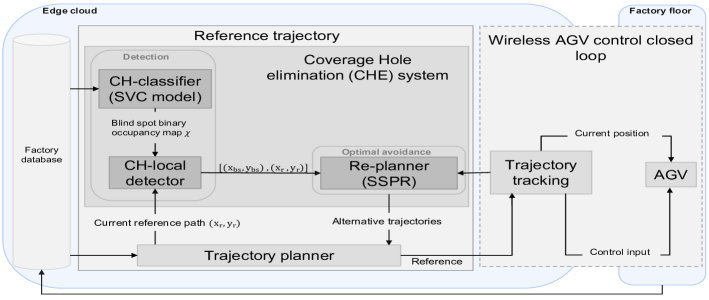
Figure. 1: Enhanced edge cloud AGV trajectories follower with the CH elimination (CBSE) system

I-A Related work

The occurrence of a coverage hole in the current AGV trajectory increases the number of successive packet drops to the tolerance limit [6], which increases the control error. If the AGV’s deviation is more from the trajectory, it will not reach the target position and leads to the controller’s instability. The author in [7] proposed a system to detect the coverage hole by the drone without transmitting a user report via a backhaul link. The Unmanned aerial vehicle (UAV) has two modes as a user and as a base station. The UAV-as-user measures the received signal power and switches the UAV to the second mode when a coverage hole is detected. The author in [8] proposed a goal-oriented communication system based on the adaptive data rate aiming to control gain improvement. The author has modeled the packet delay and information freshness. Based on this, the wireless networked control system is optimized using an adaptive data rate. The author in [9] proposes Multi-Link Connectivity (MLC) to support highly reliable, low-latency wireless links. The goal-oriented communication can be used as a solution for power map optimization. However, this conditions the knowledge of the signal strength map. The received signal strength map can be estimated via stochastic or deterministic indoor propagation model [10]. The stochastic model has a low estimation accuracy since the exact indoor geometry is not considered. The deterministic method, like the ray tracing method, has a high accuracy level as the stochastic however, this method has relatively high computational time. The trajectory planning algorithms such as Probabilistic Road-maps (PRM), which use a sampled environment map, can effectively find the shortest trajectory from the start to the target position via search algorithms [11]. The detected coverage hole positions can be iteratively added to the sampled trajectory search map to find the optimal coverage-hole-free trajectory. In [12], the author proposed the avoidance concept with Bézier curve optimization for an unknown binary map environment via a trajectory re-direction around the blocked position using the close-set positions before and behind the blocked position. So in this work, the proposed trajectory re-plan algorithm finds the second optimal trajectory as an alternative trajectory, which describes the shortest coverage-hole-free trajectory to the target position.

I-B Contribution and organization of the paper

The effect of coverage holes on AGV trajectory acquisition requires coverage hole position detection and an avoidance strategy. So this work proposes an ML-binary coverage hole map construction for the whole industry layout map iterative considering the layout or wireless transmission parameter change. So it is a binary representation of the detected coverage or non-coverage hole positions. Then, the coverage hole avoidance strategy proposes via an alternative trajectory re-planning algorithm. The trajectory re-planner maintains that the alternative trajectory is the second optimal trajectory in the sampled environment map. To the author’s knowledge, such a coverage hole elimination system for edge cloud wireless trajectory control has yet to be proposed.

Section 2 provides an overview and a detailed description of the enhanced edge cloud AGV trajectories via the coverage hole elimination (CHE) system. Section 3 describes the implementation of the binary coverage hole map construction. Furthermore, the performances of coverage hole detection are analyzed. Section 4 presents the performance of trajectory tracking considering the re-planned trajectory. Finally, in Section 5, the paper is summarized.

II System Model

The Figure 1 describes the co-located Coverage Hole Elimination (CHE) system in the AGV wireless trajectory following. Each AGV is assisted via a wireless trajectory follower to track a predefined trajectory from a start position to a target position on the factory floor within a given time $T$. The data is exchanged between the edge cloud and the industrial floor via wireless communication. The trajectory planner determines the optimal reference trajectory positions $(x_{r},y_{r})$, and the corresponding reference interpolated trajectories $T_{r}$ in the $(x,y)$-industrial coordinate system. A trajectory planner and follower are located in the edge cloud. Each AGV receives the necessary trajectory control information to follow the reference trajectory. The proposed CHE system targets to detect the position of the CH in the current AGV reference trajectory and to provide optimal alternative trajectories. The sample time interval of the CHE system is $dt$. The coverage hole should be detected and avoided at each $k^{th}$ time step. The AGV obtains the control input from the trajectory follower at each $k^{th}$ time step. The industry layout is represented in the edge cloud as a binary map. The black pixels represent blocked positions, which cannot be entered by AGV, whereas the white pixels represent the free AGV-working area 5a. After coverage hole detection, the binary Coverage Hole (CH) map is constructed. Based on the CH-local detector response, the current reference path is updated via the trajectory re-planner generating the alternative CH-free trajectory as a reference input for trajectories follower. The reference trajectories $T_{r}$ consist of the reference trajectory positions $(x_{r},y_{r})$ in $(x,y)$-industry area coordinates, AGV orientation to the $x$-axis $(\theta_{c})$ and the reference linear as well as angular velocity $(v_{r},\omega_{r})$. The CH classifier constructs the CH binary map. There are two classes of receiver power: The positions with a receiving power below the sensitivity threshold of the receiver are assigned to the CH-class $(y=0)$. Otherwise, the position with sufficient receiving power above the receiver’s sensitivity threshold is categorized as the non-CH-class $(y=1)$. The industry map can be represented as a CH binary map $\chi$ using each position’s class assignment. So the position with the CH-class is represented as a black pixel in the binary map. And the position with the non-CH-class is described as a white pixel. As shown in Figure 1, the CH detection is performed in two steps. First, the CH classifier should be able to assign the industry positions after training to two classes $\hat{y}\in\{0,1\}$. Then, a binary CH map $\chi$ can be created using industry position class assignments. Second, considering the current CH binary map can determine the local detector if the current reference trajectory contains any CH. Then, the position of the CH $(x_{bs},y_{bs})$ should be submitted to the trajectories re-planner. That means the AGV has prior information about the CH position, which can occur after a time interval Look-Ahead Time (LAT) in reference positions. The trajectories re-planner creates alternative optimal reference trajectories considering the LAT between the current AGV position at the time step $k$ and the detected CH position at the time step $k_{bs}$. Then updated reference trajectories are utilized at the trajectories follower to return a corresponding control input to AGV to minimize the error between the current AGV position and the reference position $(x_{r},y_{r},\theta_{r})$. The input information for the CH classifier is obtained from the industry database. This information should include the current industry conditions and the available RF-propagation information. Therefore, at each iteration $k^{th}$, the CHE should detect the CH in the current reference trajectory and then avoid them accordingly.

III Coverage hole detection

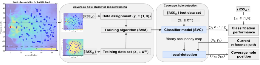
Figure. 2: CH classifier model (SVC), CH binary map construction, CH local-detection in the current reference path.

As shown in Figure 2, the possible position of the CH on the reference trajectory is determined in two steps. In the first step, a trained binary classifier model should detect the CH positions using support vector machine approach SVM. Each $i^{th}$ position has true class assignments ${y}\in\{0,1\}$ and detected class assignments from the classifier model $\hat{y}_{i}\in\{0,1\}$ in the training phase. Then, detected class assignments in the classifier test phase are considered to create the binary CH map. The second step is local-determining the CH in the current reference trajectory. The detected CH coordinate position $(x_{bs},y_{bs})$ should be forwarded to the trajectories re-planner. The industry database has information for each position on the industry floor. This information is intended to keep the available information about the RF propagation at each time, the industry layout the operating frequency, the transmitter position, the transmitter height, and the mean RF path-loss at each position. However, the machine learning classifier will consider the RF signal loss by the multi-path and shadow fading as a binary CH map. That means the trained classifier should find the correct position class assignment based on the data vector for each position. The Support Vector Classifier (SVC) is trained with true position assignments ${y}\in\{0,1\}$ based on the Received Signal Strength (RSS) map in Non-Line-of-Sight (NLOS) propagation model. Each $i^{th}$ position in the industry map will be described by a features vector $X_{i}$ in an m-dimensional feature space $R^{m}$. These features are provided as input information to the classifier for each position from the industry database. It should contain the RF transmission parameter and the available RF industry propagation conditions at each position using QUAsi Deterministic RadIo channel GenerAtor (QuaDRiGa) channel model in the industrial environment, [13]. After that, the unlabeled data set is described as a matrix $[X_{ij}]_{n\times m};\ (i=1:n)$ observation positions, and $(j=1:m)$ with $m$ is the number of features. Each $i^{th}$ observation position should be assigned to one of the two classes $y_{i}=\{0,1\}$. The class assignments $y$ are obtained from the received signal power map, including multi-path and shadow fading effects. Therefore, the training and validation phase determines the nonlinear hyperplane parameter. So the trained SVC can separate the positions of the industrial map in the m-dimensional features space $R^{m}$ using the labeled data set $[X_{i},y_{i}]$. The trained SVC should then be able to provide the correct position assignment $\hat{y}_{i}\in\{0,1\}$ using the test data set. The SVC response $\hat{y}_{i}$ describes binary position assignments that can be represented in the $(x,y)$ industry coordinate as a CH binary map. In the second step, the current AGV reference trajectory $(x_{r},y_{r})\ \text{at}\ \text{each time step \ }(k=0:\frac{T}{dt})$ is checked to determine if it has the potential to contain a CH. As illustrated in Figure 2, we have implemented the $\text{RSS}_{\text{pl}}$ map with consideration of the mean path-loss values using the empirical industrial channel model and the $\text{RSS}_{\text{sf}}$ map with consideration of the shadow and multi-path fading propagation effects. Both power maps in Figure 2 include a transmitter (red point) and multi-random distributed receivers (blue points) in an industry layout [13]. The input information $[X_{ij}]_{n\times m}$ is extracted from the $\text{RSS}_{\text{pl}}$ maps for the model training as well as for model testing. However, the position assigning in two categories $y_{i}\in\{0,1\}$ are obtained from the $\text{RSS}_{\text{sf}}$ map. The labeled test data set is also necessary to analyze the model performance by comparing the correct class assignment $y_{i}$ from the $\text{RSS}_{\text{sf}}$ map and the class assignments form the classifier $\hat{y}_{i}$. The separation of the two classes requires a nonlinear hyperplane feature space $R^{m}$ using Radial Basis Kernel (RBK) kernel. The penalty parameter in the SVC represents the inverse effect of the regularization parameter. The penalty parameter and kernel parameter are determined by L-fold cross-validation.

III-A Channel measurement

For a specific industry layout, the received signal power can be changed depending on several parameters, e.g., the variation of the height and the position of the transmitter, as well as the operating frequency and the distance to the transmitter. The mean path-loss value under change of these parameter changes should obtain at the model training from the path-loss map $\text{RSS}_{\text{pl}}$ map where $\text{RSS}_{\text{pl}}$ map is obtained considering Hata’s model in the QuaDRiGa industrial scenario. Furthermore, the data assignment is done from the $\text{RSS}_{\text{sf}}$ industrial map considering the shadowing effect as well as the multi-path effect. A random decrease in the signal strength occurs due to reflections, scattering from metallic surfaces, and multiple duplicates of the transmitted signal arrive. At the receiver, multiple paths lead to variations in the received signal strength. consequently a CH can occur in the $\text{RSS}_{\text{sf}}$ coverage map. As shown in Figure 2, the area around $(25,-20)$ is the industry $\text{RSS}_{\text{sf}}$ map with height loss of received signal power. Although, in the $\text{RSS}_{\text{pl}}$ map, this wireless channel loss does not appear in this area. The training data set is assigned with the correct position assignments via the $\text{RSS}{{}_{\text{P}_{\text{sf}}}}$ value. After that, the trained SVC should be able to assign CH positions as a positive class based on the available input information from the industry floor. As in Figure 2 show, the QuaDRiGa,[13], is used to create the RSS map; the red position is the transmitter with multiple randomly distributed receivers.

III-B Coverage hole detection performance

Since the CH classifier is used to separate imbalanced binary classes based on the available database information. The Receiver Operating Characteristic (ROC) curve is proposed to determine the operating point for the classifier model as shown in Figure 3. The true positive and the false positive CH class ”0” prediction rate is calculated with a variable prediction threshold. However, with the optimal threshold selection, the overfitting problem is avoided. On the other side, the trade-off between true and false decisions, the CH, is established. The free-CH area can be reduced if the CH false alarm detection is higher. The classifier has 0.97 Area Under Curve (AUC), which means that our classifier has the potential to predict the CH class correctly but still needs to find the optimal operation point which balances the false and true positive rate. The geometric mean between the false positive rate (FPR) and the true positive rate (TPR) is used to detect it. The operation point of the classifier is determined with 87$\%$ true positive rate as shown inFigure 3 as a red point. Nevertheless, it is accompanied by a 2$\%$ false positive CH prediction rate. However, as shown in Figure 4, the classifier performance is analyzed regarding the CH class so that the CH detection metrics are extracted from the classification confusion matrix. As expected, the classifier model can predict the CH class with a true positive rate $\text{TPR}=\frac{TP}{TP+FN}=71.7\%$. However, this is also accompanied by the false positive CH prediction rate $\text{FPR}=\frac{FP}{TN+FP}=1.8\%$. The increase in the accuracy of CH prediction is achieved with an increased prediction rate of false alarm, which reduces the working space of AGV. Nevertheless, this trade-off between TPR and FPR is limited within the ROC curve.

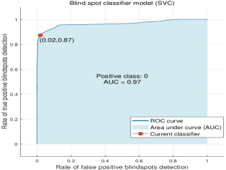
Figure. 3: Receiver operating characteristic (ROC) of the trained model

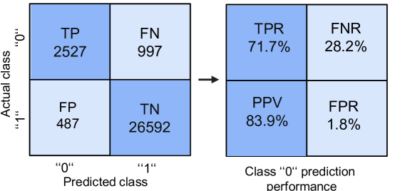
Figure. 4: Confusion matrix of the model test and CH detection performance; TP: true positive, FN: false negative.

IV Coverage hole avoidance

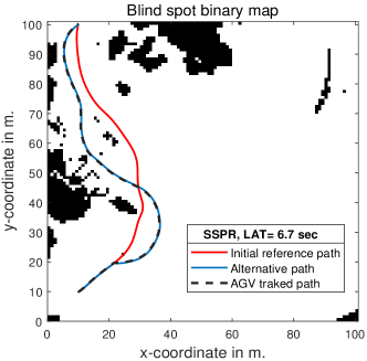
(a)

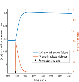
(b)

Figure. 5: Trajectories planning, re-planning, and following.

When a CH occurs in the current $(x,y)$-reference trajectory, the trajectories re-planner should find alternative optimal reference trajectories based on the updated CH binary map from the CH classifier. The trajectory re-planner should find the optimal trajectory re-routing start $SP_{re}$ to the initial target position, considering the LAT between the current AGV position and the CH position. Then the alternative trajectory positions should interpolate as $(x_{r},y_{r})$ and from it should calculate the appropriate reference AGV orientation $\theta_{r}$, the linear as well as the winkle velocity $(v_{r},w_{r})$.

IV-A Trajectory planner using PRM

Using PRM the optimal initial reference trajectory is generated. A search algorithm A-Star (A*) can find an optimal trajectory with minimal length in the PRM map under given start and target positions. The implementations of PRM are categorized into two phases a preparation phase and a query phase. In the preparation phase, a PRM map is constructed using generated random nodes $N$ in the industry map’s free AGV workspace and the connection from each node to its nearest neighbors by a straight line distance smaller than the radius $D_{max}$. The possible edges $E$ between nodes $N$ build the PRM map. Then a graph search is performed using A* in PRM map to find optimal trajectory points. Therefore, the reference trajectories are all predefined trajectory information as reference data extracted from $(x,y)$-trajectory points using the trajectory interpolation optimization. The linear and angular velocity should be customized under the technical conditions of the AGV. The cubic Basis Spline (B-spline) interpolation with Bézier function $\Psi(\cdot)$ can interpolate the variable length trajectory segments [14]. So, each segment is optimized with the Bézier curve.

IV-B Trajectories re-planner using SSPR

The optimization of the alternative trajectory is accomplished considering the look-ahead time. The look-ahead time defines the time range in which the system should find an optimal alternative. The algorithm finds the optimal alternative trajectory in the corresponding PRM map based on the current CH binary map $\chi$. Then, using the proposed Start Selection Path Re-planning (SSPR) algorithms a start position for the trajectory re-route $SP_{re}(t=t_{re})$ should be determined to provide a shorter alternative trajectory from the initial start position to the target position. As illustrated in 5a, CH positions are classified at the time step $k$, and the CH binary map is updated. A start position for trajectory re-routing is planned within the look-ahead time. The alternative optimization method guarantees that the AGV follows the first optimal trajectory within a specific time before starting the avoidance process. 5a presented a CH binary map $\chi(k)$ as an example of the classifier output at the time step $k$. The initial trajectory, which is presented in red, is planned in the previous coverage hole binary map $\chi(k-1)$; thereby, the position at $(20,21)$ was assigned to the CH-free workspace. Then, the CH map is updated at the next time step $(k)$, and a coverage hole is determined at $(20,21)$. The CH detector gives the CH position at time step $k_{bs}$ to the trajectories re-planner.

IV-C Trajectory re-planning performance

This section analyzes the performance of the SSPR. The AGV should avoid the CH position and reach the target position with an acceptable trajectory coordinate error. Under the condition of the AGV speed limitation $v_{max}$, the re-planning performance depends on the LAT is analyzed, as can be seen in Figure 6. This is expected that greater LAT provides more trajectory re-routing possibilities. The optimal alternative trajectory strongly depends on LAT and is getting reduced with increased LAT; if we make a CH detection earlier, we gain more possibilities to achieve more optimization at CH avoidance. Conversely, The LAT depends on how often the CH on the AGV trajectory occurs and disappears. In Figure 6, the analysis of multiple LAT is executed at $10$ simulations, and the average trajectory length is plotted. The randomly distributed node position is changed. Thus the PRM map is updated at each experiment due to the change of node positions. The target position remains the same in all experiments. It is clear that at larger LAT, the additional distance due to the trajectory re-route is reduced, and the alternative trajectory is minimized. Furthermore, in Figure 6 is shown that with the increase of the road map parameter $N$ and $D_{max}$ the alternative trajectory length is minimized for the same remaining LAT. Nevertheless, the increase of road map parameters is limited because of the computation resources and the real-time system requirements. Consequently, the earlier the coverage hole is identified, the shorter the alternative trajectory can be found. But if the coverage hole position is assigned to the free AGV workspace after the re-route trajectory to start. Then, the LAT should decrease since the multiple re-routing increases the trajectories following coordinate error. However, the multiple re-routing can be optimized by adjusting the PRM map parameters and the probability of coverage hole occurrence and disappearance. For highly dynamic RF propagation changes, the map parameters should increase to avoid the coverage hole considering the reduction of the alternative trajectory length and the tracked trajectory coordinates error.

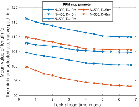
Figure. 6: The alternative trajectory length with various LAT.

V Conclusion

The proposed CHE system can detect and avoid the coverage hole. We evaluate the performance of coverage hole elimination in wireless controlled AGV use case in an industry environment. With environment layout dependence, the trained SVC model can identify the coverage hole position with high detection performance. Then, the detected coverage hole is successfully avoided via the suggested SSPR trajectory re-planner algorithm. The AGV follows the optimal alternative trajectory and reaches the target position. The larger LAT can improve coverage hole avoidance performance considering the AGV trajectory length. Moreover, the re-planning performance regarding the alternative trajectory length can also be enhanced by increasing the PRM map parameters. However, the PRM map parameter increase is constrained due to the computational edge cloud resources and real-time conditions. Nevertheless, the LAT should adjust with the coverage hole change frequency because the unnecessary avoidance with larger LAT can increase the AGV coordinate error.

References

- [1] S. Dipesh and M. Axay, “Discrete-time sliding mode controller subject to real-time fractional delays and packet losses for networked control system,” 2017.
- [2] H.-W. Liang, C.-H. Ho, L.-S. Chen, W.-H. Chung, S.-Y. Yuan, and S.-Y. Kuo, “Coverage hole detection in cellular networks with deterministic propagation model,” in 2016 2nd International Conference on Intelligent Green Building and Smart Grid (IGBSG), 2016.
- [3] A. Galindo-Serrano, B. Sayrac, S. Ben Jemaa, J. Riihijärvi, and P. Mähönen, “Automated coverage hole detection for cellular networks using radio environment maps,” 2013.
- [4] R. Jurdi, J. G. Andrews, D. Parsons, and R. W. Heath, “Identifying coverage holes: Where to densify?” in 2017 51st Asilomar Conference on Signals, Systems, and Computers, 2017.
- [5] S. Melnyk, S. Tayade, M. Zarour, and H. Schotten, “Wireless industrial communication and control system: Ai assisted blind spot detection-and-avoidance for agvs,” 2022.
- [6] S. Tayade, P. Rost, A. Mäder, and H. Schotten, “Cloud control agv over rayleigh fading channel - the faster the better,” 2019.
- [7] S. A. Al-Ahmed, M. Z. Shakir, and S. A. R. Zaidi, “Optimal 3d uav base station placement by considering autonomous coverage hole detection, wireless backhaul and user demand,” 2020.
- [8] P. M. d. S. Ana, N. Marchenko, B. Soret, and P. Popovski, “Goal-oriented wireless communication for a remotely controlled autonomous guided vehicle,” IEEE Wireless Communications, 2023.
- [9] M. Ehrig, M. Petri, V. Sark, A. G. Tesfay, S. Melnyk, H. Schotten, W. Anwar, N. Franchi, G. Fettweis, and N. Marchenko, “Reliable wireless communication and positioning enabling mobile control and safety applications in industrial environments,” in 2017 IEEE International Conference on Industrial Technology (ICIT), 2017.
- [10] D. Romero and S.-J. Kim, “Radio map estimation: A data-driven approach to spectrum cartography,” IEEE Signal Processing Magazine, 2022.
- [11] S. Alarabi, C. Luo, and M. Santora, “A prm approach to path planning with obstacle avoidance of an autonomous robot,” in 2022 8th International Conference on Automation, Robotics and Applications (ICARA), 2022.
- [12] J. Li and C. Yang, “Auv path planning based on improved rrt and bezier curve optimization,” in 2020 IEEE International Conference on Mechatronics and Automation (ICMA), 2020.
- [13] S. Jaeckel, N. Turay, L. Raschkowski, L. Thiele, R. Vuohtoniemi, M. Sonkki, V. Hovinen, F. Burkhardt, P. Karunakaran, and T. Heyn, “Industrial indoor measurements from 2-6 ghz for the 3gpp-nr and quadriga channel model,” 2019.
- [14] P. E. Koch and K. Wang, “The introduction of b-splines to trajectory planning for robot manipulators,” Department of numerical mathematics, 1988.